| Issue |
A&A
Volume 653, September 2021
|
|
|---|---|---|
| Article Number | A73 | |
| Number of page(s) | 16 | |
| Section | Planets and planetary systems | |
| DOI | https://doi.org/10.1051/0004-6361/202140569 | |
| Published online | 10 September 2021 | |
Into the storm: diving into the winds of the ultra-hot Jupiter WASP-76 b with HARPS and ESPRESSO
1
Observatoire astronomique de l’Université de Genève,
Chemin Pegasi 51b,
1290
Versoix, Switzerland
e-mail: julia.seidel@unige.ch
2
Department of Physics, and Institute for Research on Exoplanets, Université de Montréal,
Montréal,
H3T 1J4, Canada
3
Lund Observatory, Box 43,
Sölvegatan 27,
22100
Lund, Sweden
4
INAF – Osservatorio Astrofisico di Arcetri,
Largo E. Fermi 5,
50125
Florence, Italy
5
Université Grenoble Alpes, CNRS, IPAG,
38000
Grenoble, France
6
Instituto de Astrofísica e Ciências do Espaço, CAUP, Universidade do Porto, Rua das Estrelas,
4150-762
Porto, Portugal
7
Departamento de Física e Astronomia, Faculdade de Ciências, Universidade do Porto, Rua do Campo Alegre,
4169-007
Porto, Portugal
8
Physikalisches Institut & NCCR PlanetS, Universität Bern,
3012
Bern, Switzerland
9
INAF – Osservatorio Astronomico di Brera,
Via E. Bianchi 46,
23807
Merate (LC), Italy
10
Centro de Astrobiología (CAB, CSIC-INTA), Departamento de Astrofísica, ESAC campus 28692 Villanueva de la Cañada,
Madrid, Spain
11
INAF – Osservatorio Astronomico di Trieste,
via Tiepolo 11,
34143
Trieste, Italy
12
European Southern Observatory (ESO) – Alonso de Cordova 3107,
Vitacura, Santiago, Chile
13
Instituto de Astrofísica de Canarias,
Via Lactea sn,
38200,
La Laguna,
Tenerife, Spain
14
Centro de Astrofísica, Universidade do Porto,
Rua das Estrelas,
4150-762
Porto, Portugal
15
Instituto de Astrofísica e Ciências do Espaço, Faculdade de Ciências da Universidade de Lisboa,
Campo Grande,
1749-016
Lisboa, Portugal
16
INAF – Osservatorio Astrofisico di Torino,
Strada Osservatorio,
20 10025
Pino Torinese (TO), Italy
17
Centro de Astrobiología (CSIC-INTA),
Ctra. de Ajalvir km 4,
28850,
Torrejón de Ardoz,
Madrid, Spain
18
Institute for Fundamental Physics (IFPU),
Via Beirut 2,
34151
Grignano TS, Italy
19
Departamento de Astrofísica, Universidad de La Laguna,
38200
San Cristobal de La Laguna, Spain
20
Leiden Observatory, Leiden University,
Postbus 9513,
2300 RA
Leiden, The Netherlands
Received:
15
February
2021
Accepted:
20
July
2021
Context. Despite swift progress in the characterisation of exoplanet atmospheres in composition and structure, the study of atmospheric dynamics has not progressed at the same speed. While theoretical models have been developed to describe the lower layers of the atmosphere, and independently, the exosphere, little is known about the intermediate layers up to the thermosphere.
Aims. We aim to provide a clearer picture of atmospheric dynamics for the class of ultra-hot Jupiters, which are highly irradiated gas giants, based on the example of WASP-76 b.
Methods. We jointly analysed two datasets that were obtained with the HARPS and ESPRESSO spectrographs to interpret the resolved planetary sodium doublet. We then applied the MERC code, which retrieves wind patterns, speeds, and temperature profiles on the line shape of the sodium doublet. An updated version of MERC, with added planetary rotation, also provides the possibility of modelling the latitude dependence of the wind patterns.
Results. We retrieve the highest Bayesian evidence for an isothermal atmosphere, interpreted as a mean temperature of 3389 ± 227 K, a uniform day- to nightside wind of 5.5−2.0+1.4 km s−1 in the lower atmosphere with a vertical wind in the upper atmosphere of 22.7−4.1+4.9 km s−1, switching atmospheric wind patterns at 10−3 bar above the reference surface pressure (10 bar).
Conclusions. Our results for WASP-76 b are compatible with previous studies of the lower atmospheric dynamics of WASP-76 b and other ultra-hot Jupiters. They highlight the need for vertical winds in the intermediate atmosphere above the layers probed by global circulation model studies to explain the line broadening of the sodium doublet in this planet. This work demonstrates the capability of exploiting the resolved spectral line shapes to observationally constrain possible wind patterns in exoplanet atmospheres. This is an invaluable input to more sophisticated 3D atmospheric models in the future.
Key words: planets and satellites: atmospheres / planets and satellites: individual: WASP-76 b / techniques: spectroscopic / line: profiles / methods: data analysis
© ESO 2021
1 Introduction
The study of hot Jupiters is revealing a more and more detailed picture of their atmospheric composition. Through transmission spectroscopy, the existence of a wide range of atoms, ions, and molecules in hot Jupiter atmospheres has been inferred (e.g. Evans et al. 2018; Casasayas-Barris et al. 2019; Hoeijmakers et al. 2019, 2020; Tabernero et al. 2021), and established results were revised withhigher resolution (Casasayas-Barris et al. 2021). We can also detect clouds and hazes (e.g. Powell et al. 2019; Parmentier et al. 2021; Gao et al. 2020; Barstow 2020; Allart et al. 2020), the thermal structure of the atmosphere (e.g. Line et al. 2016; Evans et al. 2018; Gibson et al. 2020; Yan et al. 2020; Baxter et al. 2020), even chemical abundances of the detected elements (e.g. Line et al. 2014; Brogi & Line 2019; Pino et al. 2020), and condensation of iron (Ehrenreich et al. 2020; Borsa et al. 2021).
The first attempt of directly measuring atmospheric winds based on prior theoretical work (Knutson et al. 2008) was performed with the CO band of HD 209458 b. It found a blueshift of 2 km s−1 compared tothe systemic velocity, indicating a day- to nightside wind (Snellen et al. 2010). Similarly, studying the bands of CO and H2O in the exoplanet β Pic b, Snellen et al. (2014) found a rotational velocity of vrot = 25 ± 3 km s−1. The conceptual proof of this technique started further studies that constrained the rotational speed in the lower atmosphere of hot Jupiters, most of them consistent with the tidally locked nature of these planets (Louden & Wheatley 2015; Brogi et al. 2016).
The sodium doublet is especially well suited to bridge the missing pressure regions between the lower atmosphere that is probed withmolecular bands and the exosphere. It is a resonant doublet and probes the terminator up until the thermosphere in high resolution (Wyttenbach et al. 2015). Based on this result, the survey called Hot Exoplanet Atmospheres Resolved with Transmission Spectroscopy (HEARTS) was created and has provided a number of interesting datasets for the study of atmosphericwinds in high resolution (Wyttenbach et al. 2017; Seidel et al. 2019, 2020a,c; Hoeijmakers et al. 2020). With the possibility of resolving the line shape of single spectral lines from high-resolution transmission spectra, vertical layers below the thermosphere have become accessible through the sodium doublet and similar lines. For example, the Balmer lines have recently been used by Wyttenbach et al. (2020) to study Parker winds and rotational broadening in the ultra-hot Jupiter KELT-9 b and by Cauley et al. (2021) to study the rotational velocity of the ultra-hot Jupiter WASP-33 b. While Wyttenbach et al. (2020) reported zonal wind speeds consistent with planetary rotation for KELT-9 b, Cauley et al. (2021) reported evidence of high zonal wind speeds across the terminator and tentative evidence of a day- to nightside wind. Seidel et al. (2020b) combined a nested sampling algorithm with a forward model of different wind patterns to retrieve the line shape of the sodium doublet for HD 189733 b, thus exploring the full parameter space created by the wind speed, direction, temperature, and continuum level. The retrieval revealed a high velocity of an outwards expanding wind in the intermediate layers of the atmosphere that drives the atmospheric mass-loss in the exosphere.
Probing the lower atmosphere using the iron signature in WASP-76 b, Ehrenreich et al. (2020) measured a combination of planetary rotation and day- to nightside winds with ESPRESSO1. Revisiting the data on WASP-76 b taken with HARPS2, Kesseli & Snellen (2021) were able to confirm the results with the same technique even on the less precise HARPS data, opening up an avenue to revisit HARPS data for a multiude of similar exoplanets. The sodium doublet of WASP-76 b, first detected by Seidel et al. (2019), was recently observed with ESPRESSO,which provided an unparalleled precision of the line shape with a single transit (Tabernero et al. 2021). Based on this work, we study the atmospheric winds in WASP-76 b through the sodium doublet, probing the atmosphere up to the thermosphere, with the MERC retrieval code (Seidel et al. 2020b).
2 WASP-76 b datasets
We used two different datasets for WASP-76 b in this study, taken with the HARPS and ESPRESSO spectrographs. The HARPS WASP-76 b sodium doublet data published in Seidel et al. (2019) are based on three transits taken as part of the HEARTS survey (ESO program 100.C-0750; PI: Ehrenreich). However, since then, the system parameters for WASP-76 were updated. We address the impact of these changes in the following section.
2.1 Revised system parameters and effect on the HARPS dataset
Since the analysis of the sodium doublet from the HARPS data for WASP-76 b (Seidel et al. 2019), a close companion to the host star was detected by Bohn et al. (2020) with a separation of 0.436 ± 0.003 arcsec and a K-band magnitude difference of 2.30 ± 0.05. In consequence, the planetary parameters were updated in Southworth et al. (2020) and Ehrenreich et al. (2020). This analysis uses the new parameters from Table 1 with the stellar companion, instead of the values used by Seidel et al. (2019) from the discovery paper of West et al. (2016). The change in parameters can affect the relative velocities of the system, the star, and the planet and thus lead to a different line shape. We subsequently decided to re-analyse the HARPS dataset. The two velocities used in building the transmission spectrum that can affect the line shape are the semi-amplitude of the stellar radical velocities (RVs), K⋆, and the systemic velocity, vsys, which are both taken from Ehrenreich et al. (2020), see Table 1. The parameters were verified in Tabernero et al. (2021), who created a 2D map of the sodium detection for the dataset we used here, which clearly shows the planet trace in the stellar rest frame (Tabernero et al. 2021, Fig. 5). An analysis of the effect of the planetary orbital velocity on the results we present is provided in Appendix B, which shows that the broadening of the lines cannot stem from imprecise values of the orbital parameters.
We reduced the data in the same way as Seidel et al. (2019), but with the updated system parameters. We used the 2D echelle spectral images produced by the HARPS Data Reduction Pipeline (DRS v3.5) and discarded 15 exposures in night 3 that were affected by cirrus clouds, just as in Seidel et al. (2019). We then applied molecfit (Smette et al. 2015; Kausch et al. 2015; Allart et al. 2017) to correct for tellurics and shifted all spectra to the stellar rest frame. We combined all out-of-transit spectra to the normalised master-out and extracted the planetary signal by dividing each in-transit spectrum with the master-out. Lastly, we created the transmission spectrum by shifting the in-transit spectra into the planetary rest frame and summed over them for a sufficient signal-to-noise ratio (S/N) to detect the sodium feature. Figure 1 shows the comparison between the spectrum as presented in Seidel et al. (2019) and the new analysis with the updated parameters. The difference between the two datasets is mainly driven by the updated values for the radii. The new dataset is also shown in the upper panel of Fig. 2. While the changes are less than 1% compared to the spectrum published by Seidel et al. (2019), both lines of the sodium doublet are fainter and narrower than before. This justifies the new reduction of the data with regard to the aim of this work: to extract information from the sodium doublet line shape. However, the effect of the updated system parameters does not change any of the conclusions drawn in Seidel et al. (2019).
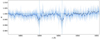 |
Fig. 1 HARPS datasets before and after the system parameter update normalised to 1. In black we show the HARPS dataset as published in Seidel et al. (2019), and in blue, we show the re-analysed dataset with the new system parameters. The verticaldashed blue lines indicate the line centre of the sodium doublet lines. |
Planetary and stellar parameters.
2.2 ESPRESSO dataset
The transmission spectrum of WASP-76 b around the sodium doublet was created from observations with the ESPRESSO spectrograph at the ESO VLT telescope in Paranal, Chile (Pepe et al. 2021). The observations were performed as part of ESO program 1102.C-0744 (ESPRESSO GTO, Ehrenreich et al. 2020; Tabernero et al. 2021). Two transits of WASP-76 b were recorded, on 3 September 2018 (night one) and 31 October 2018 (night two). For an overview of observational conditions, see Tabernero et al. (2021). In night 1, four spectra were removed due to high airmass3, and in night2, three spectra were discarded likewise.
To have planetary spectra that were obtained with the same technique (thus minimising the systematics that different methods of spectrum extraction might introduce in our analysis), we re-reduced the ESPRESSO data. The trace of the stellar sodium line centre was masked to eliminate residuals in all spectra with a window of ± 4 km s−1. Each remaining spectrum was corrected for cosmics and the transmission spectrum built following Seidel et al. (2019, 2020a). We applied molecfit (Smette et al. 2015; Kausch et al. 2015; Allart et al. 2017) to correct both nights for the effect of telluric lines and used the SKYSUB S2D output files of the DRS pipeline, which are corrected for the effect of sky emission and blaze corrected. We corrected the telluric lines down to the noise level for all airmasses and verified that no residuals are visible in the combined master spectrum. As shown by Seidel et al. (2019) for the HARPS data and by Tabernero et al. (2021) for the ESPRESSO data, the Rossiter-McLaughlin (RM) effect and centre-to-limb effects induce variations in the transmission spectra at the level of 0.04%, which is lower than the combined error on our final dataset ± 0.1%. Two possible techniques to correct for the RM effect, a numerical approximation (Wyttenbach et al. 2020) or modelling (e.g. Casasayas-Barris et al. 2019) were compared by Seidel et al. (2020b) for the hot Jupiter HD 189733 b and showed differences of approximately 0.1%, highlighting that the selection of different correction techniques introduces different systematic errors on the line shape. As shown by Casasayas-Barris et al. (2021), the RM correction also depends on the synthetic stellar spectra, and more work is needed to properly establish which model spectra should be used for RM corrections. However, for the ESPRESSO dataset, which is more sensitive to the RM effect, we masked the trace of the stellar sodium line centre, which coincides with the area of maximum impact fromthe RM effect. In conclusion, for the particular dataset presented here, a correction of the RM effect would introduce a larger uncertainty on our dataset, and we opted not to correct for this effect in the following, but to minimise it through masking.
Because of interference patterns created by Coudé train optics in ESPRESSO, the combined transmission spectrum shows sinusoidal noise (wiggles) instead of a straight base line (Allart et al. 2020; Tabernero et al. 2021). A sinusoidal fit was performed on the final transmission spectrum for each night to correct for this feature. We combined both nights and both orders containing the sodium doublet (116 and 117) and show the resulting final transmission spectrum in the middle panel of Fig. 2. The independent re-analysis of the ESPRESSO transmission spectrum is compatible with the spectrum presented in Tabernero et al. (2021).
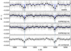 |
Fig. 2 Overview of the sodium doublet transmission spectra used in this work, normalised to 0 with the added contribution of the obscure disk of the planet. The disk contribution depends on the white-light radius and is therefore only a best-effort approximation for the real continuum in the order of the sodium doublet. Because the same radius is also used for the retrieval, this has no effect on our conclusions. Top panel: HARPS spectrum from Seidel et al. (2019) reprocessed with the updatedsystem parameters. Centre panels: ESPRESSO spectrum for each night. Bottom panel: all three datasets combined. The line centres of the sodium lines are indicated as dashed vertical blue lines, and the line spread function of the respective instrument is shown as a blue graph. |
2.3 Combined dataset and compatibility
The combined HARPS dataset and the ESPRESSO datasets for both nights can be found in Fig. 2. ESPRESSO has a higher throughput and is installed on a larger telescope than HARPS. Depending on the sky conditions, it is therefore expected that three to four HARPS transits, as in our HARPS dataset, are equivalent to one ESPRESSO transit. While the line shapes are roughly reproduced in all three datasets, the datasets show a difference in line depth. As already analysed by Seidel et al. (2019) for the HARPS dataset, the three combined HARPS nights were affected by thin cloud cover and thus varying line depths that had to be corrected for. While the line depths within the HARPS dataset were subsequently compatible, the uncertainty of HARPS is comparatively large. The two nights of ESPRESSO data re-analysed here were first studied by Tabernero et al. (2021), who found an average line depth of 0.417 ± 0.035% in night 1 and 0.270 ± 0.028% in night 2 (see overview in Table 2). In consequence, the three datasets show no visible variation in line shape when rescaled beyond what is expected from uncertainties, but they differ in line depth. Stellar activity was monitored for the HARPS dataset with simultaneous photometric observations (Seidel et al. 2019) and for the ESPRESSO dataset thorugh the Ca II H and K lines, again showing no stellar activity that could account for the differing line depths. Alternatively, the difference could stem from a change in mean atmospheric temperature between the nights and thus a change in transit depth. Therefore the value retrieved for the mean temperature of the atmosphere should be seen as a mean value and upper boundary for the real temperature of the atmosphere (see Sect. 4). Additionally, to reduce the effect of temporal temperature variations, the three datasets were combined toobtain a more precise dataset.
Because the doublet lines are much broader than the line spread functions of the instruments in question (12, 11, and13 times wider from top to bottom in Fig. 2), we can re-bin the ESPRESSO data (R ~138 000) on the lower-resolution HARPS wavelength grid (R ~ 115 000) and combine the three datasets of similar resolution (combined HARPS data, and ESPRESSO nights 1 and 2). We weighted each dataset with the respective mean S/N over the order of the sodium doublet: 48.58, 61.20, and 53.39, corresponding to a fractionof 29.77, 37.51, and 32.72% in the combined transmission spectrum. The resulting combined transmission spectrum of the sodium doublet, which is comprised of the three equivalent datasets and used in the rest of this work, is shown in the lower panel of Fig. 2.
A possible caveat for the study of line shapes is Doppler-smearing, which is introduced by the continuous change of the orbital velocity of the planet during one exposure (Ridden-Harper et al. 2016; Wyttenbach et al. 2020; Cauley et al. 2021)and the line spread function of the instrument. The exposure times for the HARPS datasets and ESPRESSSO night 2 were 300 s on average, and for ESPRESSO night 1, the exposure time was 600 s. The instrument and telescope overheads, and thus the time between exposures, is 32 s for HARPS and 68 s for ESPRESSO. We estimate the maximum Doppler-smear of the planet orbital velocity from the exposure times at 2.4 km s−1 for the HARPS and night 2 ESPRESSO dataset, and 4.7 km s−1 for the night 1 ESPRESSO dataset. This means that the mean smear over the entire exposure is approximately one resolution element andaffects the data for this particular system little, but we address the additional uncertainty in the discussion. MERC directly accounts for the instrument resolution.
Relative absorption depth atmospheric sodium, both lines combined.
3 Updates to MERC
MERC (Seidel et al. 2020b) combines a nested-sampling retrieval algorithm with a forward model to produce theoretical line profiles and then compare them with the provided dataset. The forward model includes Doppler-broadening by a variety of global wind patterns, which are described below. The algorithm provides the Bayesian evidence  for each forward model and the median of the marginalised posterior distributions of the parameters, the best-fit parameters, within the set parameter space. The difference in Bayesian evidence
  then ranks the models between each other and shows the significance of the selection of one model over another through the Jeffrey scale (see Table 3 or Trotta 2008 and Skilling 2006). Table 3 together with a more in-depth explanation can also be found in Lavie et al. (2017) or Seidel et al. (2020b). Further details on MERC can be found in Seidel et al. (2020b).
Empirical scale to judge the evidence when comparing two models M0 and M1, called a ‘Jeffrey scale’.
3.1 Wind patterns
MERC can model different wind patterns impacting the spectral line shape and offset: a day- to nightside wind, a super-rotational wind, and a vertical wind, as well as a combination of the first two patterns in the lower atmosphere and a vertical wind in the upper atmosphere.
To implement these wind patterns in the line of sight (LOS), we calculated the wind broadening for one atmospheric slice in the LOS (see Seidel et al. 2020b for details or Fig. 3 for an illustration). The atmospheric slice was divided into cells, and each atmospheric profile in the respective cells was Doppler-shifted by the corresponding wind velocity component in the LOS. Summing over the cells to create the slice then led to an overall Doppler broadening. For a full 3D treatment of the atmospheric dynamics, this procedure would have to be repeated for each cell through wich the light passes,which requires computing times incompatible with a nested-sampling retrieval approach. Therefore Seidel et al. (2020b) used the symmetry of the proposed wind patterns and rotated the atmospheric slice by 2π or a fraction thereof to obtain the full atmosphere. While preferable for computational reasons, this approach restricts the wind patterns to constant wind speeds in latitude throughout the planet atmosphere. Additionally, co-rotation of the atmosphere with the planet rotation cannot be accounted for because it depends on latitude. Especially for a super-rotational or day- to nightside wind, work with global circulation models (GCMs) has shown that they have a more jet-like structure for hot Jupiters, with stronger winds at the equator than at the poles (e.g. Showman et al. 2009).
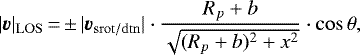
Subsequently, we updated MERC and introduced the possibility for a solid-body-like latitude dependence of the super-rotational or day- to nightside wind speeds, as was implemented for Parker winds and rotation in Wyttenbach et al. (2020). The verticalwind only expands the atmosphere, regardless of the latitude. This approach produces the strongest wind at the equator and imposes a reduction of zonal winds to zero at the poles. The new calculation of the wind speed in the LOS, compared to Eq. (7) from Seidel et al. (2020b), is then
 (1)
(1)
where θ is the angle between the equator and the radial vector to the current cell (an approximation of its latitude), Rp is the planet white-light radius, b is the impact factor (the current position above the surface in z, see Fig. 2 in Seidel et al. (2020b) for a visualisation), and x is the current position of the cell along the LOS, expressing the position of the cell in Cartesian coordinates. In this treatment of atmospheric slices, the zonal winds are not parallel to the equator, but point towards the anti-stellar point (see Fig. 3). This geometry has no effect on the LOS component of the velocity, which drives the line broadening and is only an artefact of the chosen geometry.
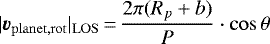
The planetary rotation, assuming the planet is tidally locked, adds a velocity of
 (2)
(2)
to each cell, with P as the rotation period. The planetary rotation is added to all models with or without winds.
The twovelocity grids from the planetary rotation and the wind were co-added to obtain the LOS velocity. Because the stored atmosphericslice has to be broadened by the LOS wind speed in each cell, this computation cannot be made for each possible angle θ. We introduced a sector variable s that slices each quarter of each hemisphere (see Fig. 3 or Wyttenbach et al. 2020) into sub-sectors. The velocities were therefore only calculated once for each sector and then rotated by  . θ is defined as the angle in the centre of the sector. We tested different numbers of sectors (between 3 and 48 in steps of 3) and found changes of less than 1% in the final model spectrum for s ≥ 9. In consequence, all models in this work were calculated with nine sectors. The approach of introducing latitude-dependent sectors introduces a new dimension to MERC and thus a quasi-3D calculation of the atmosphere at the terminator probed by transmission spectroscopy. However, some assumptions were still made for the sake of reducing the computational cost: we assumed that the planet is tidally locked and that the planetary obliquity is perpendicular to the orbital plane. Both these assumptions are reasonable for exoplanets as close to their host star as WASP-76 b (West et al. 2016).
Additionally, as already mentioned in Seidel et al. (2020b), the zonal wind patterns, now including the planetary rotation, are not axisymmetric with the rotational axis of the planet, but spherically symmetric. Because we integrated over the entire terminator and are only interested in the LOS components, this has no significant effect on the resulting line profile. On a similar note, for a proper time-resolved treatment of the day- to nightside wind, we would have to take into account the orbital inclination and angle of the current position (ζ in Fig. 3 of Ehrenreich et al. 2020) because the real symmetry axis is the connector between star and planet in a tidally locked system, and not the LOS. The cos(i) of the orbital inclination is close to 1 and was subsequently ignored, and the orbital angle can be disregarded as well because we integrated over the entire transit, averaging attransit centre where the real symmetry axis and the LOS are parallel.
We applied the latitude-dependent wind patterns as well as the unmodulated constant wind patterns to determine whether the winds inWASP-76 b show a tendency to be restricted into zonal jets or if a more uniform wind flow along the terminator is preferred. We took the planetary rotation into account for all retrievals in this work.
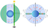 |
Fig. 3 Illustration of the implementation of the day- to nightside wind (updated version of Fig. 3 from Seidel et al. 2020b). All other zonal wind patterns are implemented in the same fashion. A polar view of the atmosphere is shown on the left and an equatorial view on the right. The wind direction and strength are indicated in blue, and the direction and strength of the rotational velocity of the planet is shown in red. Dashed black lines indicate the border between sectors. For illustration purposes, we set s = 3, see text. Left: dotted arrows indicate the direction of the velocities. The extinction coefficient is calculated in altitude along the z-axis and then transposed in the x-direction along the LOS (dark green cells). The LOS is then iterated upward in z until the top of the atmosphere is reached, and all values are saved in a 2D grid (here visualised as a slice in light green). In each bin of the 2D grid, the combined velocity of wind and planet rotation and the broadened profile are calculated and stored (see Seidel et al. 2020b for more details). Right: position of the observer. Points indicate a flow towards the observer, crosses indicate a flow away from the observer. The process described on the left is repeated foreach sector, where the velocities are adjusted for the latitude via Eq. (1) and then rotated by π∕s (or π∕2s, depending on the symmetry) to create the full atmosphere. In this simplification of the atmosphere, the wind is not parallel to the equator, but points towards the anti-stellar point. This reduces calculation time significantly because it reduces the problem from 3D to 2D for each sector, with the extinction coefficient only calculated once in 1D, while providing quasi-3D insights into the wind structure. |
Overview of the different prior ranges of the models.
3.2 Degeneracies and the continuum
We did not modify the approach of Seidel et al. (2020b) regarding the fit to the spectral continuum, where we followed the simple description of the degeneracy between the sodium abundance and the pressure scaling as presented in Lecavelier Des Etangs et al. (2008) and Heng et al. (2015) and retrieved a degeneracy parameter NaX and the temperature T to set the continuum level of the flux. While this is an important subject to address for exoplanets with richer chemistry and an interest in the correct retrieval of varying abundances, we fixed the abundance to a constant value, which is a common approach in modelling hot-Jupiter atmospheres (Lecavelier Des Etangs et al. 2008; Agúndez et al. 2014; Steinrueck et al. 2019). Nonetheless, the effect of varying the sodium abundance on the results is discussed qualitatively in Sect. 4. With respect to the temperature, we explored a deviation from an isothermal treatment of the atmosphere by introducing a temperature gradient to verify if the common assumption of an isothermal atmosphere can also be applied here. Lastly,Seidel et al. (2020b) reported that MERC retrieved the best-fit parameters in two stages, first on the continuum, far from the line doublet, to obtain the appropriate range of possible parameters for NaX and T, and then onthe line to further constrain the continuum parameters and the wind speeds and directions. The update to the code presented here includes additional parallelisation and now allows selecting a slightly wider wavelength range of three times the full width at half maximum (FWHM), thus combining the line core with enough of the continuum to eliminate the need for a two-tier retrieval as used by Seidel et al. (2020b). Further details on degeneracies, line broadening types, and the continuum parameter can be found in the first paper on MERC Seidel et al. (2020b), and in the works on which the forward model is based (Ehrenreich et al. 2006; Pino et al. 2018).
4 Retrieval results
We applied MERC with its updates presented in Sect. 3 to the combined HARPS and ESPRESSO dataset presented in Sect. 2. We examined multiple forward models, all with added planetary rotation: an isothermal temperature profile (iso), a temperature gradient (T grad), both with no added winds, and an isothermal temperature profile combined with various wind patterns: a uniform day to nightside wind (called dtn in the following tables and figures), a cos θ dependent day- to nightside wind (dtncos θ), a uniform super-rotational wind (srot), a cos θ dependent super-rotational wind (srotcos θ), a vertical wind (ver), and lastly, a two-layer approach with either a super-rotational or day- to nightside wind in the lower atmosphere combined with a vertical wind in the upper atmosphere. The switch between atmospheric layers was tested at different pressures (dtncos θ, ver; dtn, ver; srot, ver).
One of the most prominent features of Bayesian retrieval is the application of priors. Priors set the boundary conditions for the parameter space and allow adding knowledge of the physical properties to the numerical analysis of the fits. The priors used in this work are listed in Table 4. The priors for the mean isothermal temperature Tiso and the degenerate continuum parameter NaX were set to exclude non-physical results in terms of temperature, pressure, and sodium abundance. The velocity parameters were set more freely, from the lowest value close to zero to velocity ranges far beyond the escape velocity. The velocity priors were set each in both directions and had no sign. The effect of the priors is discussed in Sect. 4. The plotting range of the posteriors in Appendix A was selected for visibility and does not reflect the entire prior range.
The isothermal model without added winds (but taking planetary rotation into account) is the simplest model and served as our base to calculate the significance of the Bayesian evidence for all other models with  . The Bayesian evidence of each model, as well as the significance of the model according to the Jeffrey scale in Table 3, is shown in Table 5 with a visual representation of the strength of evidence in Fig. 4. The posteriors from the nested-sampling retrieval as corner plots are shown in Appendix A, with the mean values at the top of each column and the parameters retrieved with the highest Bayesian evidence marked in blue.
4.1 Temperature profiles
Comparing the Bayesian evidence of the temperature gradient model to the isothermal model shows that there is not sufficient evidence for one model over the other. The temperature gradient was approximated through a base and a top temperature, where the base is the continuum level of the data and the top the highest probed layer of the atmosphere. The temperature-gradient model converges towards the isothermal solution and is then punished for the additional parameter with lower Bayesian evidence (see Fig. A.2). We therefore used an isothermal temperature profile throughout all other retrieved models, which should only be interpreted as an upper limit mean temperature in light of the variation of the datasetsin line depths and the intrinsic nature of transit observations as a mean over the terminator. The application of a homogeneous mean temperature profile, however, does not rule out the existence of a temperature gradient that might be temporally variable and averaged over in the combined dataset. The combined dataset is needed to properly constrain winds in the atmosphere, the main goal of this work. A more in-depth treatment of temporal temperature variations in the atmosphere of WASP-76 b is deferred to future work. The range of retrieved temperatures for all models is higher than the equilibrium temperature of WASP-76 b. The approximate temperature of 3300−3400 K for the hottest part in the higher layers of the atmosphere retrieved for the models presented here is even higher than expected from Ehrenreich et al. (2020). The temperature retrieval is driven by the line depth and thus affected by the level of the continuum and the accuracy of the line depth and system parameters. In MERC, we take Rayleigh scattering into account, but do not account for the effects of H− opacity (Gandhi et al. 2020) on the continuum level for computational reasons. Therefore the temperature should be interpreted as an upper boundary only. However, even as an upper limit, the temperature remains curiously high, and the effect and likely cause are discussed in Sect. 5.
Comparison of the different models.
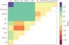 |
Fig. 4 Visualisation of the difference in Bayesian evidence of Table 5. The colour scale indicates
|

4.2 Latitude-dependent wind patterns
Of all models presented in this section, only those with a day- to nightside wind or a super-rotational wind could show a latitude dependence. In most studies using GCMs, these wind patterns are restricted to bands along the equator (called jets) and weaken towards the poles (Showman et al. 2009, 2018; Parmentier et al. 2018). We approximated this behaviour by introducing a solid-body rotation dependence (cos θ) to the wind pattern, as described in Sect. 3.1. The wind speeds retrieved for all models in this section (2− 4 km s−1) are compatible with GCM studies (e.g. Showman et al. 2018; Parmentier et al. 2018). Comparing the Bayesian evidence between the uniform wind patterns and their cos θ counterparts shows no evidence for a better fit with a jet-like structure for super-rotational wind ( ), weak evidence for a better fit with a uniform wind pattern for the day- to nightside wind over a jet-like structure (
 ), and weak evidence for a better fit when the uniform wind pattern is applied to the lower atmosphere (
 ) in the combined wind patterns (lower day- to nightside wind and upper vertical wind). Although the evidence for a preference of the uniform wind patterns with no latitude dependence is only weak (see Table 3), it shows that for WASP-76 b, the winds are likely not primarily restricted in jets and flow more evenly across the terminator. However, this does not rule out any jet-like structure in the lower atmosphere of WASP-76 b, especially a multi-jet scenario as seen for Jupiter (Liu & Schneider 2010) that would look identical to a wide jet when integrated over the atmosphere.
4.3 Uniform wind patterns
All tested uniform wind patterns show moderate to strong evidence for a better fit when compared to the base model without winds (see Table 5). A vertical wind throughout the atmosphere at  is not only preferred over the base model (
 , strong evidence), but also over the next-best wind pattern (
 , strong evidence). This indicates that a strong vertical wind is needed to create the broadened line shape, which cannot be created solely from a moderate day- to nightside or super-rotational wind at the retrieved velocities of 2− 4 km s−1.
Comparing the day- to nightside wind with the super-rotational wind, it appears at first glance that the super-rotational wind is preferred ( , weak evidence). This serves as an excellent reminder to be aware of model limitations and blind application of nested sampling. The super-rotational broadening splits the sodium doublet into two sub-peaks, one that is redshifted at the morning terminator, and another that is blueshifted at the evening terminator, which creates a strong broadening in the wings. Consequently, every part of the atmosphere receives some shift, and the line depth is severely decreased by a strong super-rotational wind. While this would be anexcellent fit for a very broad but shallow sodium doublet, it does not work similarly for the deep sodium lines in this dataset. To subsequently offset the lack of unshifted parts of the atmosphere that would sit at the centre, the retrieval increases the temperature, which is the main driver of the line depth. This leads to retrieved temperatures well beyond 4000 K, which are not physically sensible for an ultra-hot Jupiter with the system parameters of WASP-76 b (see Table 1 and the posterior distributions in Appendix A) and are ruled out via the prior. Additional evidence for this line of thought comes from the combined two-layer models, in which part of the atmosphere has the sodium lines unshifted, but broadened by vertical wind, and part of the atmosphere is dominated by either a day- to nightside or a super-rotational wind. In this scenario, the day- to nightside wind is preferred over the super-rotational wind, as predicted (
 , moderate evidence within the uncertainty). With ESPRESSO, the resolution would be sufficient to show this split into two peaks of the sodium line, provided that the S/N is sufficient and that super-rotation is the dominant wind pattern in the atmosphere and not super-imposed with other wind patterns that leave parts of the atmosphere at net zero wind speed (e.g. a combination with day- tonightside winds).
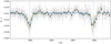 |
Fig. 5 Best fit of isothermal line retrieval with an added day- to nightside wind in the lower atmosphere without a cos θ dependence and a vertical wind in the upper atmosphere in blue on the dataset in grey. The day- to nightside wind without a cos θ dependence throughout the atmosphere (moderate evidence) is shown for comparison purposes in orange. According to the Jeffrey scale, which is logarithmic, the best-fit model in blue has a probability higher than an order of magnitude than the moderate evidence model in orange. The data were binned by ten bins in black for better visualisation. The sodium doublet line centres are indicated by dashed vertical blue lines. |
4.4 Two-layer patterns
To approximate a more realistic structure of exoplanet atmospheres, we divided the atmosphere into a lower and higher atmosphere and allowed for different wind patterns in the two layers. In the lower layer, we applied a day- to nightside or a super-rotational wind, and a vertical wind in the higher layer. The first question was where to set the boundary between the two layers. As shown by Seidel et al. (2020b), the additional parameter for the switch of layers introduces too many variables so that proper convergence of the retrieval is not possible. Because of the log-scale of the pressure, which serves as a proxy for relative height above the surface, only a few values for the layer switch are sensible and a restriction beyond an order of magnitude estimate is not necessary, especially because there will most likely be a transition zone between the wind patterns. Assuming a surface pressure at the continuum of 10 bar, as is customary in the literature (e.g. Lecavelier Des Etangs et al. 2008; Agúndez et al. 2014; Line et al. 2014; Pino et al. 2018), we explored layer switches at 10−3 bar, 10−4 bar, and 10−5 bar. 10−3 bar compared to the continuum pressure because the lowest value corresponds to the location of the jets found for hot Jupiters in GCM modelling (Showman et al. 2009). We therefore know a priori that zonal winds dominate the atmosphere below this threshold. As is evident from the posterior plots for a layer switch at 10−5 bar (see Figs. A.7 and A.10), this switch is set too high and cannot properly constrain the upper layer. The preferred switch of layers, if any, should therefore lie between these two values. A switch between dynamical regimes at 10−3 bar, as predicted by GCM results, is preferred with at least  (strong evidence within the uncertainty of the results) independently of the assumed dynamics in the lower layer (dtn, srot, or ver). We thus fixed the pressure switch at 10−3 bar for the two-layer pattern models.
Of these models, a uniform day- to nightside wind has the highest evidence in the lower atmosphere,with moderate evidence over the super-rotational wind and weak evidence over a cos θ latitude dependence of the wind, which are the next-best two models. Therefore the model with a vertical wind in the upper and day- to nightside wind in the lower atmosphere is preferred over any other model. The preference for a uniform wind in the lower atmosphere over the cos θ latitude dependence implies that if the winds in the lower atmosphere in WASP-76 b are restricted to a jet-like band at the equator, it has to be relatively broad, spanning at least farther in latitude than a scaling through solid-body rotation suggests (> 30°). The higher evidence for a day- to nightside wind over a super-rotational wind stems from a visible offset of the sodium doublet to the blue, as highlighted in Tabernero et al. (2021), where a median offset of − 5.4 ± 2.6 for all detected lines was found. The posterior distribution of the best-fit model is shown in Fig. 6, and the resulting retrieved transmission spectrum is overplotted on the data in Fig. 5. The day- to nightside wind has a speed of  , while the vertical wind shows speeds of
  . Because we took planetary rotation into account under the assumption of tidal locking, these wind speeds are not upper limits, but constrain the possible wind speeds in the atmosphere of WASP-76 b to within 30% for the lower layer and 20% for the upper layer (see uncertainty of the retrieval). However, as discussed in Sect. 2.3, because of the necessary exposure time, the lines will be smeared by one resolution element in each direction, which increases the error on the wind speed for the radial outwards wind by roughly 10% (dominated by the width) and also by roughly 10% for the day- to nightside wind (lower absolute wind speed, but dominated by the line position). This has no effect on the overall conclusions on the wind patterns we present in the studied system.
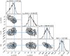 |
Fig. 6 Posterior distribution of isothermal line retrieval with an added day- to nightside wind in the lower atmosphere and a vertical wind in the upper atmosphere. The change of layers was set at p = 10−3 bar, with thepressure at the surface set to P0 = 10 bar. |
5 Discussion
Recently, Ehrenreich et al. (2020) studied WASP-76 b using ESPRESSO through the atomic iron signature and found a significant asymmetry between the first and second half of the transit, leading to a one-sided shift of the signature. At first, the iron detection shows no shift during ingress and then moves to a constant blueshift of 11.0 ± 0.7 km s−1. Taking planetary rotation into account, they concluded that the lower atmosphere of WASP-76 b shows a day- to nightside wind of 5.3 km s−1. The result, a best-fit to the sodium doublet with a day- to nightside wind of  , is compatible with their findings in the lower atmosphere in which iron is present (at pressures higher than the micro bar level). This result is driven by the detected offset of the lines to the blue by ~ 5 km s−1 in Tabernero et al. (2021), which is confirmed in this work and can either be induced by a day- to nightside wind over the entire planet or by a super-rotational wind with condensation of sodium on the nightside. Because the condensation temperature of sodium (50% condensated with T ≈ 1000 K; Lodders 2003) is much too low for the nightside temperature of an ultra-hot Jupiter (Parmentier et al. 2018), we rule out an asymmetrical super-rotational wind. A similar offset observation was made for WASP-121 b, another ultra-hot Jupiter (Borsa et al. 2021). In the our analysis, we neglected the RM effect, which was taken into account by Ehrenreich et al. (2020). The verification of the wind pattern from Ehrenreich et al. (2020) thus additionally confirms the negligible RM effect for this particular system.
None of the studies analysing wind patterns in the lower atmosphere, however, are capable of probing what occurs in the intermediate atmosphere between the mass-loss in the exosphere and the various zonal wind patterns in the lower atmosphere. We show through atmospheric retrieval that these layers are connected by a strong vertical wind of  for WASP-76 b. Seidel et al. (2020b) observed a similar phenomenon for HD 189733 b that was later confirmed through independent observations by Keles et al. (2020). This vertical wind can either be an outward-expanding wind, where the material does not descend towards lower atmospheric layers, or the vertical parts of large cell-like structures, where the upper zonal arm of the cell is inthe thermosphere. Assuming this large cell-like structure, the upper zonal arm would not affect the sodium-line shape because sodium would be ionised at these altitudes and only recombine in the downwards vertial arm of the cell. Because of the nature of transmission observations over the terminator, these two wind patterns cannot be distinguished. In the case of HD 189733 b, the interaction of ions in the lower atmosphere with the surprisingly strong estimated magnetic field (Cauley et al. 2019)could be a possible explanation of a purely expanding wind (Seidel et al. 2020b), dragging neutral sodium upwards. For WASP-76 b, no indirect magnetic field strength estimates are available, but if the same mechanism is at work for this exoplanet, the magnetic field strength should be comparable to the magnetic field strengths observed in the sample of Cauley et al. (2019), orders of magnitude higher than the magnetic field of Jupiter.
The observed vertical wind, regardless of its origin, feeds material up to the thermosphere, where it could be further heated and escape through hydrodynamic escape. This has not been directly observed for WASP-76 b, but strong planetary winds, bordering on hydrodynamical escape, are predicted for WASP-76 b (see Salz et al. 2016, Fig. 3, for log10ΦG(WASP - 76 b) ≈ 13). This is compatible with the results by Seidel et al. (2019), who showed that sodium expands far above the surface, but velocities remain just below the escape velocity for WASP-76 b. The revised escape velocity with the updated planetary radius and mass is 41 ± 1 km s−1, significantly higher than the vertical wind speeds retrieved for sodium. Therefore the vertical wind is a transport mechanism for material to the thermosphere, but not the direct driver of atmospheric escape. However, it is important to note that due to the integration over the entire atmosphere, variations in wind speed within the two atmospheric regimes are not accounted for, but rather, a mean wind velocity is derived. Whether the expanding wind gains momentum with height, driven by processes in the thermosphere, or fuels it itself is consequently unclear.
While the result provides compelling evidence for the case of strong vertical winds in the upper atmosphere, there are competing ideas to explain the broad line shape of sodium in hot Jupiters: for a low sodium abundance, the sodium might form an optically thin cloud high up in the atmosphere, producing a very broad feature. However, this is dependent on the line ratio and has been shown not to apply to WASP-76 b (Gebek & Oza 2020). Additionally, more complex temperature profiles might apply for WASP-76 b, varying in latitude or longitude, which the retrieval cannot account for. While the line shape is sensitive to the temperature through thermal broadening, it cannot produce the line shape observed forthe sodium doublet in hot Jupiters (Wyttenbach et al. 2015; Huang et al. 2017; Seidel et al. 2020b). Another caveat is the assumption of local thermodynamic equilibrium (LTE), which excludes any non-LTE effects that might affect the line shape. Recently, Fisher & Heng (2019) quantified this assumption and highlighted that currently, LTE and non-LTE atmospheres cannot be distinguished. This strengthens the case for strong vertical winds.
Zhang (2020) recently reviewed the current knowledge regarding temperature profiles for ultra-hot Jupiters (defined as having equilibrium temperatures higher than ~2200 K). Temperature inversions were confirmed through emission observations for KELT-9 b (Pino et al. 2020), WASP-121 b (Evans et al. 2017; Bourrier et al. 2020), a planet similar to WASP-76 b, for WASP-18 b (Sheppard et al. 2017), for WASP-189 b (Yan et al. 2020), and WASP-33 b (Haynes et al. 2015; Nugroho et al. 2017). Nonetheless, temperature inversions are not established as an unequivocal feature of ultra-hot Jupiters because some, for example, WASP-12 b and WASP-103 b, have spectra consistent with blackbody radiation, suggesting isothermal atmospheres (Arcangeli et al. 2018; Parmentier et al. 2018; Kreidberg et al. 2018). As a caveat, these observations stem from WFC3, and the black-body spectra in the covered band could also be explained with a temperature inversion, which might attribute these outliers to observational limitations. TiO and VO have been suggested as two possible drivers of thermal inversion by heating the upper atmosphere (Hubeny et al. 2003; Fortney et al. 2008), although discussions of the mechanisms of thermal inversions are still ongoing (Mollière et al. 2015; Lothringer & Barman 2019; Gandhi & Madhusudhan 2019), and atomic metals were suggested as an alternative inversion agent (e.g. ZrO) (Lothringer & Barman 2019; Tabernero et al. 2021). This additional caveat is especially important because some of the mentioned works on temperature inversions are disputed, for example in WASP-33 b, where the features seen in Nugroho et al. (2017) could not be confirmed by Herman et al. (2020), but were again seen tentatively in Serindag et al. (2021). Nugroho et al. (2020) even found iron lines in emission, strengthening the case for additional causes of inversion layers in addition to TiO and VO. Assuming TiO and VO as the main drivers of inversion layers, Tabernero et al. (2021) ruled out TiO and VO down to a level of < 10 ppm, and in line with the reasoning from Nugroho et al. (2017), they suggested that TiO and VO might be hidden below stronger features or be very weak, with another possibility being that both are transported from the dayside to the nightside by a day- to nightside wind where they condense out of the atmosphere. While the retrieval presented here cannot and does not aim to shed light on the detailed temperature structure of WASP-76 b, an isothermal temperature profile does not disagree with the current knowledge about ultra-hot Jupiters. The suggestion of day- to nightside winds from Tabernero et al. (2021) to explain their findings on TiO and VO is consistent with our results for the winds.
As already mentioned in Sect. 4, the temperature retrieved here is surprisingly high when compared to the equilibrium temperature and would lead to the ionisation of sodium, which we estimated with FastChem (Stock et al. 2018). At the equilibrium temperature of the planet, sodium remains in its neutral state at a fairly constant abundance up to 10−5 bar, whereas at temperatures of 3300 K and beyond, sodium ionises far lower in the atmosphere, in disagreement with the detected and confirmed sodium feature. This apparent inconsistency, where the retrieved temperature implicates an improbably high initial sodium abundance to compensate for ionisation, merits a more detailed investigation. Instead of concluding that a non-physical initial sodium abundance has to be present in ultra-hot Jupiters, it is more likely that vertical winds, such as found here, which interact with the sodium in the atmosphere,inevitably alter the density profile of sodium, away from a hydrostatic description of the atmosphere. In practice, the modified density profile will inflate the line depth, which has to then be compensated for with a higher homogeneous sodium abundance in the hydrostatic model. In conclusion, while a change in density profile has no significant effect on the line shape and therefore our results, winds will modify density profiles. Studies hoping to fit sodium abundances in low or high resolution have to account for the density profile of sodium generated by mid-latitude winds such as detected in this work.
6 Conclusions
We have studied winds in the atmosphere of the ultra-hot Jupiter WASP-76 b through its resolved sodium doublet. The transmission spectrum in the wavelength range of the sodium doublet is composed of two nights of ESPRESSO data (Ehrenreich et al. 2020; Tabernero et al. 2021) and the reprocessed HARPS dataset published by Seidel et al. (2019), which were combined thorugh S/N weighing. We introduced an update to the MERC code from Seidel et al. (2020b), which now takes planetary rotation into account and allows latitude-dependent zonal wind patterns. We found no evidence that a temperature gradient is preferred over an isothermal atmosphere. We combined the isothermal temperature profile with a uniform day- to nightside wind, a latitude-dependent day- to nightside wind, a uniform super-rotational wind, a latitude-dependent super-rotational wind, a vertical wind, and a two-layer combinationof either day- to nightside or super-rotational winds in the lower and the vertical wind in the upper atmosphere.
The best-fit model is a uniform day- to nightside wind in the lower atmosphere of  with a vertical, most likely mainly expanding wind in the upper atmosphere of
  . Assuming a surface pressure of P0 = 10 bar, the switch between the two layers is set at p = 10−3 bar. For all models, we retrieved an isothermal temperature between 3300−3400 K and discussed that this overestimate is most likely a direct result of the effect of winds on the density profile of sodium in WASP-76 b. This is an important caveat for future studies regarding the fit of abundances from spectral lines. Our findings are compatible with the current literature on the wind dynamics of lower atmospheres and temperature profiles of hot and ultra-hot Jupiters, especially with previous work on WASP-76 b. Ehrenreich et al. (2020) used the time-resolved iron detection with ESPRESSO and reported a day- to nightside wind of 5.3 km s−1. This result is corroborated by our findings in this study. Additionally, we demonstrated a need for vertical winds in the intermediate atmosphere of these highly irradiated gas giants through their broadened features.
Our work proves the effectiveness of direct retrieval on resolved spectral lines to constrain possible wind patterns as input for more in-depth theoretical studies and the crucial role of high-resolution spectrographs for atmospheric characterisation. Our findings show a clear need for more detailed climate simulations that take the higher layers of the atmosphere into account to draw a clear picture of the atmospheres of ultra-hot exoplanets.
Acknowledgements
This project has received funding from the European Research Council (ERC) under the European Union’s Horizon 2020 research and innovation programme (project FOUR ACES; grant agreement No. 724427). This work has been carried out within the frame of the National Centre for Competence in Research ‘PlanetS’ supported by the Swiss National Science Foundation (SNSF). This work was supported by FCT – Fundação para a Ciência e Tecnologia (FCT) through national funds and by FEDER through COMPETE2020 – Programa Operacional Competitividade e Internacionalização by these grants: UID/FIS/04434/2019; UIDB/04434/2020; UIDP/04434/2020; PTDC/FIS-AST/32113/2017 & POCI-01-0145-FEDER-032113; PTDC/FIS-AST/28953/2017 & POCI-01-0145-FEDER-028953. V.A. acknowledges the support from FCT through Investigador FCT contract nr. IF/00650/2015/CP1273/CT0001. N.J.N. acknowledges support form the following projects: UIDB/04434/2020 & UIDP/04434/2020, CERN/FIS-PAR/0037/2019, PTDC/FIS-OUT/29048/2017, COMPETE2020: POCI-01-0145-FEDER-028987 & FCT: PTDC/FIS-AST/28987/2017. The INAF authors acknowledge financial support of the Italian Ministry of Education, University, and Research with PRIN 201278X4FL and the “Progetti Premiali” funding scheme. JLB acknowledges financial support from “la Caixa” Foundation (ID 100010434) under the fellowship LCF/BQ/PI20/11760023, and from the European Union’s Horizon 2020 research and innovation programme under the Marie Skłodowska-Curie grant agreement No 847648. AW acknowledges the financial support of the SNSF by grant number P400P2_186765. SGS acknowledges the support from FCT through Investigador FCT contract nr. CEECIND/00826/2018 and POPH/FSE (EC). ODSD is supported in the form of a work contract (DL 57/2016/CP1364/CT0004) funded by FCT. We would like to thank the anonymous referee for their thorough and thoughtful comments that greatly improved the quality of the manuscript.
Appendix A Posterior distributions of the retrievals
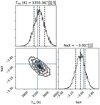 |
Fig. A.1 Posterior distribution of isothermal line retrieval. This was used as the base model to which all other scenarios were compared. |
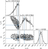 |
Fig. A.2 Posterior distribution of temperature gradient line retrieval. Tbase is at the surface of the planet, and Ttop at the top of the probed atmosphere. |
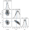 |
Fig. A.3 Posterior distribution of isothermal line retrieval with an added vertical wind constant throughout the atmosphere. |
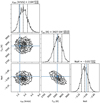 |
Fig. A.4 Posterior distribution of isothermal line retrieval with an added constant day- to nightside wind throughout the atmosphere. |
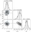 |
Fig. A.5 Posterior distribution of isothermal line retrieval with an added constant super-rotational wind throughout the atmosphere. |
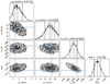 |
Fig. A.6 Posterior distribution of isothermal line retrieval with an added day- to nightside wind in the lower atmosphere and a vertical wind in the upper atmosphere. The change in the layers was set at p = 10−4 bar, with the surface pressure at P0 = 10 bar. |
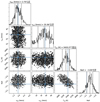 |
Fig. A.7 Posterior distribution of isothermal line retrieval with an added day- to nightside wind in the lower atmosphere and a vertical wind in the upper atmosphere. The change in the layers was set at p = 10−5 bar, with the surface pressure at P0 = 10 bar. |
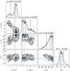 |
Fig. A.8 Posterior distribution of isothermal line retrieval with an added super-rotational side wind in the lower atmosphere and a vertical wind in the upper atmosphere. The change in the layers was set at p = 10−3 bar, with the surface pressure at P0 = 10 bar. |
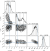 |
Fig. A.9 Posterior distribution of isothermal line retrieval with an added super-rotational side wind in the lower atmosphere and a vertical wind in the upper atmosphere. The change in the layers was set at p = 10−4 bar, with the surface pressure at P0 = 10 bar. |
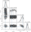 |
Fig. A.10 Posterior distribution of isothermal line retrieval with an added super-rotational side wind in the lower atmosphere and a vertical wind in the upper atmosphere. The change in the layers was set at p = 10−5 bar, with the surface pressure at P0 = 10 bar. |
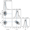 |
Fig. A.11 Posterior distribution of isothermal line retrieval with an added day- to nightside wind dependent on the latitude through cos θ. |
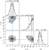 |
Fig. A.12 Posterior distribution of isothermal line retrieval with an added super-rotational wind dependent on the latitude through cos θ. |
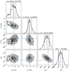 |
Fig. A.13 Posterior distribution of isothermal line retrieval with an added cos θ dependent day- to nightside wind in the lower atmosphere and a vertical wind in the upper atmosphere. The change in the layers was set at p = 10−3 bar, with the surface pressure at P0 = 10 bar. |
Appendix B Discussion of the planetary orbital velocity
To strengthen our argument that the line shape indeed stems from the dynamical structure of the exoplanet atmosphere and not from factors related to the orbital motion, we studied the effect of the planetary orbital motion (Kp) and its uncertainty on our results. In our analysis, we used the value of Kp as calculated from the stellar mass, period, and inclination by Ehrenreich et al. (2020).
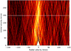 |
Fig. B.1 Kp-vsys map generated from the two ESPRESSO nights, the position of the sodium line as calculated in Ehrenreich et al. (2020) is indicated as dashed white lines. White areas stem from the masking of the data at the centre of the stellar sodium lines. Lighter colours indicate a stronger detection signal. |
However, to demonstrate the effect of Kp on the sodium doublet line shape, we also derived Kp directly from the signal of the planetary sodium (see Figure B.1). Figure B.1 shows the Kp - vsys space, where we combined the ESPRESSO transits and the two sodium lines to generate the signal. We excluded the HARPS data from this demonstration to keep re-binning at a minimum and the signal shape as precise as possible.
The map presented in Figure B.1 confirms the sodium signal that was already independently established with the HARPS spectrograph (Seidel et al. 2019) and the ESPRESSO spectrograph (Tabernero et al. 2021), and it also confirms its broad line shape. However, the map also demonstrates the difficulties encountered when Kp is directly derived from the data of single lines instead of hundreds or even thousands of spectral lines (see e.g. Hoeijmakers et al. 2020). The signal is too broad in Kp to properly derive a precise value, spanning from roughly 50 to 250 km s−1 due to the low number of available lines.
It also demonstrates that the line shape is independent of small errors on Kp because we sampled very similarly broad profiles for values of Kp varying up to 10 km s−1 from the value derived in Ehrenreich et al. (2020). The value of Kp as calculated by Ehrenreich et al. (2020) therefore is preferred to our own calculation for two reasons: it is much more precise with a value of 196.52 ± 0.94 km s−1, which translates into a maximum error at ingress and egress of ± 0.3 km s−1 (less than one ESPRESSO pixel). Additionally, in their calculation, they do not take the in-transit data into account and decoupled the calculation of Kp from any atmospheric dynamics. This makes any retrieval of the atmospheric dynamics more robust against the effect of orbital motion.
In conclusion, the derivation of Kp from our dataset has shown that the sodium signal exists and that its line shape can only be explained by broadening winds or other atmospheric dynamics. The effect of the orbital motion on our results is negligible.
References
- Agúndez, M., Parmentier, V., Venot, O., Hersant, F., & Selsis, F. 2014, A&A, 564, A73 [NASA ADS] [CrossRef] [EDP Sciences] [Google Scholar]
- Allart, R., Lovis, C., Pino, L., et al. 2017, A&A, 606, A144 [NASA ADS] [CrossRef] [EDP Sciences] [Google Scholar]
- Allart, R., Pino, L., Lovis, C., et al. 2020, A&A, 644, A155 [NASA ADS] [CrossRef] [EDP Sciences] [Google Scholar]
- Arcangeli, J., Désert, J.-M., Line, M. R., et al. 2018, ApJ, 855, L30 [NASA ADS] [CrossRef] [Google Scholar]
- Barstow, J. K. 2020, MNRAS, 497, 4183 [CrossRef] [Google Scholar]
- Baxter, C., Désert, J.-M., Parmentier, V., et al. 2020, A&A, 639, A36 [EDP Sciences] [Google Scholar]
- Bohn, A. J., Southworth, J., Ginski, C., et al. 2020, A&A, 635, A73 [NASA ADS] [CrossRef] [EDP Sciences] [Google Scholar]
- Borsa, F., Allart, R., Casasayas-Barris, N., et al. 2021, A&A, 645, A24 [EDP Sciences] [Google Scholar]
- Bourrier, V., Kitzmann, D., Kuntzer, T., et al. 2020, A&A, 637, A36 [CrossRef] [EDP Sciences] [Google Scholar]
- Brogi, M., & Line, M. R. 2019, AJ, 157, 114 [Google Scholar]
- Brogi, M., de Kok, R. J., Albrecht, S., et al. 2016, ApJ, 817, 106 [Google Scholar]
- Casasayas-Barris, N., Pallé, E., Yan, F., et al. 2019, A&A, 628, A9 [NASA ADS] [CrossRef] [EDP Sciences] [Google Scholar]
- Casasayas-Barris, N., Palle, E., Stangret, M., et al. 2021, A&A, 647, A26 [NASA ADS] [CrossRef] [EDP Sciences] [Google Scholar]
- Cauley, P. W., Shkolnik, E. L., Llama, J., & Lanza, A. F. 2019, Nat. Astron., 3, 408 [NASA ADS] [CrossRef] [Google Scholar]
- Cauley, P. W., Wang, J., Shkolnik, E. L., et al. 2021, AJ, 161, 152 [Google Scholar]
- Ehrenreich, D., Tinetti, G., Lecavelier Des Etangs, A., Vidal-Madjar, A., & Selsis, F. 2006, A&A, 448, 379 [NASA ADS] [CrossRef] [EDP Sciences] [Google Scholar]
- Ehrenreich, D., Lovis, C., Allart, R., et al. 2020, Nature, 580, 597 [Google Scholar]
- Evans, T. M., Sing, D. K., Kataria, T., et al. 2017, Nature, 548, 58 [NASA ADS] [CrossRef] [Google Scholar]
- Evans, T. M., Sing, D. K., Goyal, J. M., et al. 2018, AJ, 156, 283 [NASA ADS] [CrossRef] [Google Scholar]
- Fisher, C., & Heng, K. 2019, ApJ, 881, 25 [Google Scholar]
- Fortney, J. J., Lodders, K., Marley, M. S., & Freedman, R. S. 2008, ApJ, 678, 1419 [NASA ADS] [CrossRef] [Google Scholar]
- Gandhi, S., & Madhusudhan, N. 2019, MNRAS, 485, 5817 [Google Scholar]
- Gandhi, S., Madhusudhan, N., & Mandell, A. 2020, AJ, 159, 232 [Google Scholar]
- Gao, P., Thorngren, D. P., Lee, G. K. H., et al. 2020, Nat. Astron., 4, 951 [CrossRef] [Google Scholar]
- Gebek, A., & Oza, A. V. 2020, MNRAS, 497, 5271 [Google Scholar]
- Gibson, N. P., Merritt, S., Nugroho, S. K., et al. 2020, MNRAS, 493, 2215 [Google Scholar]
- Haynes, K., Mandell, A. M., Madhusudhan, N., Deming, D., & Knutson, H. 2015, ApJ, 806, 146 [NASA ADS] [CrossRef] [Google Scholar]
- Heng, K., Wyttenbach, A., Lavie, B., et al. 2015, ApJ, 803, L9 [Google Scholar]
- Herman, M. K., de Mooij, E. J. W., Jayawardhana, R., & Brogi, M. 2020, AJ, 160, 93 [Google Scholar]
- Hoeijmakers, H. J., Ehrenreich, D., Kitzmann, D., et al. 2019, A&A, 627, A165 [NASA ADS] [CrossRef] [EDP Sciences] [Google Scholar]
- Hoeijmakers, H. J., Seidel, J. V., Pino, L., et al. 2020, A&A, 641, A123 [CrossRef] [Google Scholar]
- Huang, C., Arras, P., Christie, D., & Li, Z.-Y. 2017, AAS Meeting Abs., 229, 301.01 [NASA ADS] [Google Scholar]
- Hubeny, I., Burrows, A., & Sudarsky, D. 2003, ApJ, 594, 1011 [Google Scholar]
- Kausch, W., Noll, S., Smette, A., et al. 2015, A&A, 576, A78 [NASA ADS] [CrossRef] [EDP Sciences] [Google Scholar]
- Keles, E., Kitzmann, D., Mallonn, M., et al. 2020, MNRAS, 498, 1023 [NASA ADS] [CrossRef] [Google Scholar]
- Kesseli, A. Y., & Snellen, I. A. G. 2021, ApJ, 908, L17 [Google Scholar]
- Knutson, H. A., Charbonneau, D., Allen, L. E., Burrows, A., & Megeath, S. T. 2008, ApJ, 673, 526 [Google Scholar]
- Kreidberg, L., Line, M. R., Parmentier, V., et al. 2018, AJ, 156, 17 [NASA ADS] [CrossRef] [Google Scholar]
- Lavie, B., Mendonça, J. M., Mordasini, C., et al. 2017, AJ, 154, 91 [Google Scholar]
- Lecavelier Des Etangs, A., Pont, F., Vidal-Madjar, A., & Sing, D. 2008, A&A, 481, L83 [NASA ADS] [CrossRef] [Google Scholar]
- Line, M. R., Fortney, J. J., Marley, M. S., & Sorahana, S. 2014, ApJ, 793, 33 [Google Scholar]
- Line, M. R., Stevenson, K. B., Bean, J., Kreidberg, L., & Fortney, J. J. 2016, AAS Meeting Abs., 227, 224.03 [NASA ADS] [Google Scholar]
- Liu, J., & Schneider, T. 2010, J. Atm. Sci., 67, 3652 [NASA ADS] [CrossRef] [Google Scholar]
- Lodders, K. 2003, ApJ, 591, 1220 [Google Scholar]
- Lothringer, J. D., & Barman, T. 2019, ApJ, 876, 69 [Google Scholar]
- Louden, T., & Wheatley, P. J. 2015, ApJ, 814, L24 [NASA ADS] [CrossRef] [Google Scholar]
- Mollière, P., van Boekel, R., Dullemond, C., Henning, T., & Mordasini, C. 2015, ApJ, 813, 47 [NASA ADS] [CrossRef] [Google Scholar]
- Nugroho, S. K., Kawahara, H., Masuda, K., et al. 2017, AJ, 154, 221 [Google Scholar]
- Nugroho, S. K., Gibson, N. P., de Mooij, E. J. W., et al. 2020, ApJ, 898, L31 [Google Scholar]
- Parmentier, V., Line, M. R., Bean, J. L., et al. 2018, A&A, 617, A110 [NASA ADS] [CrossRef] [EDP Sciences] [Google Scholar]
- Parmentier, V., Showman, A. P., & Fortney, J. J. 2021, MNRAS, 501, 78 [Google Scholar]
- Pepe, F., Cristiani, S., Rebolo, R., et al. 2021, A&A, 645, A96 [CrossRef] [EDP Sciences] [Google Scholar]
- Pino, L., Ehrenreich, D., Wyttenbach, A., et al. 2018, A&A, 612, A53 [NASA ADS] [CrossRef] [EDP Sciences] [Google Scholar]
- Pino, L., Désert, J.-M., Brogi, M., et al. 2020, ApJ, 894, L27 [Google Scholar]
- Powell, D., Louden, T., Kreidberg, L., et al. 2019, ApJ, 887, 170 [NASA ADS] [CrossRef] [Google Scholar]
- Ridden-Harper, A. R., Snellen, I. A. G., Keller, C. U., et al. 2016, A&A, 593, A129 [NASA ADS] [CrossRef] [EDP Sciences] [Google Scholar]
- Salz, M., Schneider, P. C., Czesla, S., & Schmitt, J. H. M. M. 2016, A&A, 585, L2 [NASA ADS] [CrossRef] [EDP Sciences] [Google Scholar]
- Seidel, J. V., Ehrenreich, D., Wyttenbach, A., et al. 2019, A&A, 623, A166 [NASA ADS] [CrossRef] [EDP Sciences] [Google Scholar]
- Seidel, J. V., Ehrenreich, D., Bourrier, V., et al. 2020a, A&A, 641, L7 [CrossRef] [EDP Sciences] [Google Scholar]
- Seidel, J. V., Ehrenreich, D., Pino, L., et al. 2020b, A&A, 633, A86 [NASA ADS] [CrossRef] [EDP Sciences] [Google Scholar]
- Seidel, J. V., Lendl, M., Bourrier, V., et al. 2020c, A&A, 643, A45 [CrossRef] [EDP Sciences] [Google Scholar]
- Serindag, D. B., Nugroho, S. K., Mollière, P., et al. 2021, A&A, 645, A90 [EDP Sciences] [Google Scholar]
- Sheppard, K. B., Mandell, A. M., Tamburo, P., et al. 2017, ApJ, 850, L32 [Google Scholar]
- Showman, A. P., Fortney, J. J., Lian, Y., et al. 2009, ApJ, 699, 564 [NASA ADS] [CrossRef] [Google Scholar]
- Showman, A. P., Tan, X., & Zhang, X. 2018, in AGU Fall Meeting Abstracts, 2018, P43E–3818 [Google Scholar]
- Skilling, J. 2006, Bayesian Anal., 1, 833 [Google Scholar]
- Smette, A., Sana, H., Noll, S., et al. 2015, A&A, 576, A77 [NASA ADS] [CrossRef] [EDP Sciences] [Google Scholar]
- Snellen, I. A. G., de Kok, R. J., de Mooij, E. J. W., & Albrecht, S. 2010, Nature, 465, 1049 [NASA ADS] [CrossRef] [PubMed] [Google Scholar]
- Snellen, I. A. G., Brandl, B. R., de Kok, R. J., et al. 2014, Nature, 509, 63 [NASA ADS] [CrossRef] [Google Scholar]
- Southworth, J., Bohn, A. J., Kenworthy, M. A., Ginski, C., & Mancini, L. 2020, A&A, 635, A74 [NASA ADS] [CrossRef] [EDP Sciences] [Google Scholar]
- Steinrueck, M. E., Parmentier, V., Showman, A. P., Lothringer, J. D., & Lupu, R. E. 2019, ApJ, 880, 14 [Google Scholar]
- Stock, J. W., Kitzmann, D., Patzer, A. B. C., & Sedlmayr, E. 2018, MNRAS, 479, 865 [NASA ADS] [Google Scholar]
- Tabernero, H. M., Zapatero Osorio, M. R., Allart, R., et al. 2021, A&A, 646, A158 [NASA ADS] [CrossRef] [EDP Sciences] [Google Scholar]
- Trotta, R. 2008, Contemp. Phys., 49, 71 [Google Scholar]
- West, R. G., Hellier, C., Almenara, J. M., et al. 2016, A&A, 585, A126 [NASA ADS] [CrossRef] [EDP Sciences] [Google Scholar]
- Wyttenbach, A., Ehrenreich, D., Lovis, C., Udry, S., & Pepe, F. 2015, A&A, 577, A62 [NASA ADS] [CrossRef] [EDP Sciences] [Google Scholar]
- Wyttenbach, A., Lovis, C., Ehrenreich, D., et al. 2017, A&A, 602, A36 [NASA ADS] [CrossRef] [EDP Sciences] [Google Scholar]
- Wyttenbach, A., Mollière, P., Ehrenreich, D., et al. 2020, A&A, 638, A87 [EDP Sciences] [Google Scholar]
- Yan, F., Espinoza, N., Molaverdikhani, K., et al. 2020, A&A, 642, A98 [NASA ADS] [CrossRef] [EDP Sciences] [Google Scholar]
- Zhang, X. 2020, Res. Astron. Astrophys., 20, 099 [CrossRef] [Google Scholar]
All Tables
Empirical scale to judge the evidence when comparing two models M0 and M1, called a ‘Jeffrey scale’.
All Figures
|
Fig. 1 HARPS datasets before and after the system parameter update normalised to 1. In black we show the HARPS dataset as published in Seidel et al. (2019), and in blue, we show the re-analysed dataset with the new system parameters. The verticaldashed blue lines indicate the line centre of the sodium doublet lines. |
| In the text | |
|
Fig. 2 Overview of the sodium doublet transmission spectra used in this work, normalised to 0 with the added contribution of the obscure disk of the planet. The disk contribution depends on the white-light radius and is therefore only a best-effort approximation for the real continuum in the order of the sodium doublet. Because the same radius is also used for the retrieval, this has no effect on our conclusions. Top panel: HARPS spectrum from Seidel et al. (2019) reprocessed with the updatedsystem parameters. Centre panels: ESPRESSO spectrum for each night. Bottom panel: all three datasets combined. The line centres of the sodium lines are indicated as dashed vertical blue lines, and the line spread function of the respective instrument is shown as a blue graph. |
| In the text | |
|
Fig. 3 Illustration of the implementation of the day- to nightside wind (updated version of Fig. 3 from Seidel et al. 2020b). All other zonal wind patterns are implemented in the same fashion. A polar view of the atmosphere is shown on the left and an equatorial view on the right. The wind direction and strength are indicated in blue, and the direction and strength of the rotational velocity of the planet is shown in red. Dashed black lines indicate the border between sectors. For illustration purposes, we set s = 3, see text. Left: dotted arrows indicate the direction of the velocities. The extinction coefficient is calculated in altitude along the z-axis and then transposed in the x-direction along the LOS (dark green cells). The LOS is then iterated upward in z until the top of the atmosphere is reached, and all values are saved in a 2D grid (here visualised as a slice in light green). In each bin of the 2D grid, the combined velocity of wind and planet rotation and the broadened profile are calculated and stored (see Seidel et al. 2020b for more details). Right: position of the observer. Points indicate a flow towards the observer, crosses indicate a flow away from the observer. The process described on the left is repeated foreach sector, where the velocities are adjusted for the latitude via Eq. (1) and then rotated by π∕s (or π∕2s, depending on the symmetry) to create the full atmosphere. In this simplification of the atmosphere, the wind is not parallel to the equator, but points towards the anti-stellar point. This reduces calculation time significantly because it reduces the problem from 3D to 2D for each sector, with the extinction coefficient only calculated once in 1D, while providing quasi-3D insights into the wind structure. |
| In the text | |
|
Fig. 4 Visualisation of the difference in Bayesian evidence of Table 5. The colour scale indicates
|
| In the text | |
|
Fig. 5 Best fit of isothermal line retrieval with an added day- to nightside wind in the lower atmosphere without a cos θ dependence and a vertical wind in the upper atmosphere in blue on the dataset in grey. The day- to nightside wind without a cos θ dependence throughout the atmosphere (moderate evidence) is shown for comparison purposes in orange. According to the Jeffrey scale, which is logarithmic, the best-fit model in blue has a probability higher than an order of magnitude than the moderate evidence model in orange. The data were binned by ten bins in black for better visualisation. The sodium doublet line centres are indicated by dashed vertical blue lines. |
| In the text | |
|
Fig. 6 Posterior distribution of isothermal line retrieval with an added day- to nightside wind in the lower atmosphere and a vertical wind in the upper atmosphere. The change of layers was set at p = 10−3 bar, with thepressure at the surface set to P0 = 10 bar. |
| In the text | |
|
Fig. A.1 Posterior distribution of isothermal line retrieval. This was used as the base model to which all other scenarios were compared. |
| In the text | |
|
Fig. A.2 Posterior distribution of temperature gradient line retrieval. Tbase is at the surface of the planet, and Ttop at the top of the probed atmosphere. |
| In the text | |
|
Fig. A.3 Posterior distribution of isothermal line retrieval with an added vertical wind constant throughout the atmosphere. |
| In the text | |
|
Fig. A.4 Posterior distribution of isothermal line retrieval with an added constant day- to nightside wind throughout the atmosphere. |
| In the text | |
|
Fig. A.5 Posterior distribution of isothermal line retrieval with an added constant super-rotational wind throughout the atmosphere. |
| In the text | |
|
Fig. A.6 Posterior distribution of isothermal line retrieval with an added day- to nightside wind in the lower atmosphere and a vertical wind in the upper atmosphere. The change in the layers was set at p = 10−4 bar, with the surface pressure at P0 = 10 bar. |
| In the text | |
|
Fig. A.7 Posterior distribution of isothermal line retrieval with an added day- to nightside wind in the lower atmosphere and a vertical wind in the upper atmosphere. The change in the layers was set at p = 10−5 bar, with the surface pressure at P0 = 10 bar. |
| In the text | |
|
Fig. A.8 Posterior distribution of isothermal line retrieval with an added super-rotational side wind in the lower atmosphere and a vertical wind in the upper atmosphere. The change in the layers was set at p = 10−3 bar, with the surface pressure at P0 = 10 bar. |
| In the text | |
|
Fig. A.9 Posterior distribution of isothermal line retrieval with an added super-rotational side wind in the lower atmosphere and a vertical wind in the upper atmosphere. The change in the layers was set at p = 10−4 bar, with the surface pressure at P0 = 10 bar. |
| In the text | |
|
Fig. A.10 Posterior distribution of isothermal line retrieval with an added super-rotational side wind in the lower atmosphere and a vertical wind in the upper atmosphere. The change in the layers was set at p = 10−5 bar, with the surface pressure at P0 = 10 bar. |
| In the text | |
|
Fig. A.11 Posterior distribution of isothermal line retrieval with an added day- to nightside wind dependent on the latitude through cos θ. |
| In the text | |
|
Fig. A.12 Posterior distribution of isothermal line retrieval with an added super-rotational wind dependent on the latitude through cos θ. |
| In the text | |
|
Fig. A.13 Posterior distribution of isothermal line retrieval with an added cos θ dependent day- to nightside wind in the lower atmosphere and a vertical wind in the upper atmosphere. The change in the layers was set at p = 10−3 bar, with the surface pressure at P0 = 10 bar. |
| In the text | |
|
Fig. B.1 Kp-vsys map generated from the two ESPRESSO nights, the position of the sodium line as calculated in Ehrenreich et al. (2020) is indicated as dashed white lines. White areas stem from the masking of the data at the centre of the stellar sodium lines. Lighter colours indicate a stronger detection signal. |
| In the text | |
Current usage metrics show cumulative count of Article Views (full-text article views including HTML views, PDF and ePub downloads, according to the available data) and Abstracts Views on Vision4Press platform.
Data correspond to usage on the plateform after 2015. The current usage metrics is available 48-96 hours after online publication and is updated daily on week days.
Initial download of the metrics may take a while.