| Issue |
A&A
Volume 673, May 2023
|
|
|---|---|---|
| Article Number | A125 | |
| Number of page(s) | 15 | |
| Section | Planets and planetary systems | |
| DOI | https://doi.org/10.1051/0004-6361/202245800 | |
| Published online | 17 May 2023 | |
Detection of a high-velocity sodium feature on the ultra-hot Jupiter WASP-121 b★
1
European Southern Observatory,
Alonso de Córdova 3107,
Vitacura, Región Metropolitana,
Chile
e-mail: jseidel@eso.org
2
INAF – Osservatorio Astronomico di Brera,
Via E. Bianchi 46,
23807
Merate (LC),
Italy
3
INAF – Osservatorio Astrofisico di Arcetri,
Largo E. Fermi 5,
50125
Florence,
Italy
4
Observatoire astronomique de l’Université de Gèneve,
Chemin Pegasi 51b,
1290
Versoix,
Switzerland
5
Instituto de Astrofísica de Canarias,
Via Lactea sn,
38200
La Laguna, Tenerife,
Spain
6
Centro de Astrobiología (CSIC-INTA),
Ctra. de Ajalvir km 4,
28850
Torrejón de Ardoz, Madrid,
Spain
7
Physikalisches Institut & NCCR PlanetS,
Universität Bern,
3012
Bern,
Switzerland
8
Department of Physics, and Trottier Institute for Research on Exoplanets, Université de Montréal,
Montréal
H3T 1J4,
Canada
9
INAF – Osservatorio Astronomico di Trieste,
via Tiepolo 11,
34143
Trieste,
Italy
10
Instituto de Astrofísica e Ciências do Espaço, CAUP, Universidade do Porto,
Rua das Estrelas,
4150-762
Porto,
Portugal
11
Centro de Astrofísica da Universidade do Porto,
Rua das Estrelas,
4150-762
Porto,
Portugal
12
Departamento de Física e Astronomia, Faculdade de Ciências, Universidade do Porto,
Rua do Campo Alegre,
4169-007
Porto,
Portugal
13
Institute for Fundamental Physics (IFPU),
Via Beirut 2,
34151
Grignano TS,
Italy
14
Instituto de Astrofísica e Ciências do Espaço, Faculdade de Ciências da Universidade de Lisboa,
Campo Grande,
1749-016
Lisboa,
Portugal
15
INAF – Osservatorio Astrofisico di Torino,
Strada Osservatorio,
20 10025
Pino Torinese (TO),
Italy
Received:
25
December
2022
Accepted:
10
March
2023
Context. Ultra-hot Jupiters, with their high equilibrium temperatures and resolved spectral lines, have emerged as a perfect testbed for new analysis techniques in the study of exoplanet atmospheres. In particular, the resolved sodium doublet as a resonant line has proven a powerful indicator to probe the atmospheric structure over a wide pressure range.
Aims. We aim to explore an atmospheric origin of the observed blueshifted feature next to the sodium doublet of the ultra-hot Jupiter WASP-121 b using a partial transit obtained with the 4-UT mode of ESPRESSO. We intend to study its atmospheric dynamics visible across the terminator by splitting the data into mid-transit and egress.
Methods. We explored the impact of the Rossiter-McLaughlin effect on the line shape of the sodium doublet. The partial transit is separated into one dataset centred around mid-transit and one dataset comprising the second part of the transit and egress. Lastly, the atmospheric retrieval code, Multinested Eta Retrieval Code (MERC), was applied to both datasets in order to study the imprint of atmospheric dynamics on the line shape of the sodium doublet.
Results. We determine that the blueshifted high-velocity absorption component is generated only during the egress part of the transit when a larger fraction of the day side of the planet is visible. For the egress data, MERC retrieves the blueshifted high-velocity absorption component as an equatorial day-to-night side wind across the evening limb, with no zonal winds visible on the morning terminator with weak evidence compared to a model with only vertical winds. For the mid-transit data, the observed line broadening is attributed to a vertical, radial wind.
Conclusions. We attribute the equatorial day-to-night-side wind over the evening terminator to a localised jet and restrain its existence between the substellar point and up to 10° to the terminator in longitude, an opening angle of the jet of at most 60° in latitude, and a lower boundary in altitude between [1.08, 1.15] Rp. As a hypothesis, we propose that the jet is produced by the excitation of standing planetary scale Rossby waves by stellar irradiation and subsequently broken by Kelvin-Helmholtz instabilities. Due to the partial nature of the transit, we cannot make any statements on whether the jet is truly super-rotational and one-sided or part of a symmetric day-to-night-side atmospheric wind from the hotspot.
Key words: planets and satellites: atmospheres / planets and satellites: individual: WASP-121 b / techniques: spectroscopic / methods: data analysis / line: profiles
© The Authors 2023
 Open Access article, published by EDP Sciences, under the terms of the Creative Commons Attribution License (https://creativecommons.org/licenses/by/4.0), which permits unrestricted use, distribution, and reproduction in any medium, provided the original work is properly cited.
This article is published in open access under the Subscribe to Open model. Subscribe to A&A to support open access publication.
1 Introduction
The atmospheric dynamics of our gas giant neighbours Jupiter and Saturn and their banded structure have been studied since the dawn of telescopes to help us better understand Earth’s uniqueness (Kaspi et al. 2020). With the clear advantage of fly-bys of human-made spacecraft (Smith et al. 1979) and in situ probes such as the latest mission to Jupiter with Juno (Kaspi et al. 2020), the deep structure of Jupiter’s atmosphere is remarkably well understood. However, to fully appreciate the atmospheric dynamics of gas giants, the observations of our closest planetary neighbours have to be seen in the wider context of population studies of exoplanets.
While low-resolution studies from space have paved the way with indirect wind measurements (Knutson et al. 2007; Cowan et al. 2007), ground-based observations quickly caught up: the 2 km s−1 blueshift observed in high-resolution for the CO band of HD209458 b can be credited as the first ground-based attempt to directly measure atmospheric winds in an exoplanet atmosphere (Snellen et al. 2010). They compared the observed shift with the systemic velocity of the system and concluded that the blueshift is most likely induced by a day-to-night-side wind dominating the pressure levels probed by the CO band (based on theoretical work by Knutson et al. 2008). However, this first attempt relied on integrating over the entire dataset to compensate for a low signal-to-noise ratio (S/N) leaving many degenerate solutions to the observed blueshift, most notably a possible explanation of the shift from the uncertainty of the planetary orbit (Montalto et al. 2011).
Recently, the Balmer lines have been used to probe winds beyond the thermosphere (see e.g. Wyttenbach et al. 2020, for the study of Parker winds in KELT-9 b). In Cauley et al. (2021), the offset of the line centre of the Balmer lines was mapped throughout the transit, allowing for a first-order tracing of the wind speed as a function of time. They attribute the observed shift to large zonal winds and interpret this as evidence for day-to-night-side winds, as they rule out a jet stream with elevated wind speeds. Most of these studies are conducted on hot or ultra-hot Jupiters, where the degeneracy between planetary rotation and atmospheric circulation can be broken as they are tidally locked (Louden & Wheatley 2015; Brogi et al. 2016).
One of the most powerful observational probes of atmospheric dynamics as a function of time in the lower atmosphere is the tracking of the atmospheric Doppler shift via the cross-correlation technique (Snellen et al. 2010) as first presented in Borsa et al. (2019) and Ehrenreich et al. (2020). Here, the offset from the theoretical position in velocity space is traced throughout the transit for the forest of spectral iron lines which gives us additional spatial information on different visible parts of the atmosphere (see also Kesseli & Snellen 2021; Wardenier et al. 2022). To probe a wider range of atmospheric layers in altitude, the sodium doublet, as a resonant line, has emerged as a readily available probe (Wyttenbach et al. 2015), where the Doppler-shift-induced change in line shape can be attributed to atmospheric dynamics, for instance via ( Multi-nested ETA Retrieval Code (MERC), Seidel et al. 2020b, 2021; Mounzer et al. 2022). While able to distinguish between different winds patterns based on retrievals for the first time, these works also relied on the time integration over the entire transit and could not distinguish any evolution of wind patterns based on different viewing geometries of the exoplanet atmosphere. Nonetheless, the sodium retrieval technique spanning orders of magnitude in altitude and the time-resolved CCF tracing of the lower atmosphere independently deduced a day-to-night-side wind of approximately 5 km s−1 in the lower atmosphere of the ultra-hot Jupiter WASP-76 b (Ehrenreich et al. 2020; Seidel et al. 2021) with an outwards bound wind linking to higher atmospheric layers (Seidel et al. 2021).
In this work, we study the atmospheric dynamics of WASP-121 b with MERC as a first exploration into time-resolving narrow-band transmission spectroscopy. WASP-121 b is a highly irradiated exoplanet orbiting a relatively bright F6V-type star (V = 10.4 mag, Teq = 2358 ± 52 K) with a bloated atmosphere (R = 1.753 ± 0.036 RJ, M = 1.157 ± 0.070 MJ), (Delrez et al. 2016; Bourrier et al. 2020b). Given its closeness to its host star (0.02544 ± 0.0005 AU) and the resulting high equilibrium temperature (2358 ± 52 K), it is classified as an ultra-hot Jupiter (Evans et al. 2017), a class of exoplanets most notably characterised by molecular dissociation and the resulting atomic spectral lines (Arcangeli et al. 2018; Kitzmann et al. 2018; Lothringer et al. 2018; Parmentier et al. 2018). From H2O observations with the WFC3 and STIS instruments on the Hubble Space Telescope (HST), Evans et al. (2017) inferred a temperature inversion in its day-side atmosphere. The temperature profile of both the night and day-side of this tidally locked exoplanet was then constrained in Mikal-Evans et al. (2022) and Daylan et al. (2021). They observed a difference in temperature between the day and night side of the planet of 1000 K with approximately 1500 K on the cooler night side and 2500 K on the hotter day side which then increases to over 4000 K above 10−3 bar. However, there is no significant phase shift between the brightest and substellar points, which was confirmed from TESS optical photometry in Bourrier et al. (2020b). This indicates inefficient heat transportation across the terminator and two distinct atmospheric regimes in the day and night-side realm. In Maguire et al. (2023), high-resolution ESPRESSO1 data, including the here studied 4-UT transit, are used to retrieve relative abundances and temperature pressure profiles. They find 3450 ± 160 K for pressures above 10−2 bar compatible with the previously mentioned temperature inversion, and also in line with UVES observations in Gibson et al. (2020, 2022).
A wide range of elements were identified in the transmission spectrum of WASP-121 b using ground-based data (Bourrier et al. 2020b,a; Cabot et al. 2020; Hoeijmakers et al. 2020; Gibson et al. 2020; Merritt et al. 2021; Borsa et al. 2021); for our work, these were most importantly the resolved sodium lines. Thanks to advances in high-resolution cross-correlation techniques (CCF), the non-detection of Ti and TiO (Hoeijmakers et al. 2020; Merritt et al. 2021; Wilson et al. 2021) was attributed to a depletion of Ti at the terminators (Gibson et al. 2020). Recently, Hoeijmakers et al. (2022) interpreted these trends as cold-trapping of Ti on the night side of the atmosphere, which implies a wider variety in ultra-hot Jupiter atmospheres based on slight differences in temperature or dynamical structure. Applying the cross-correlation technique to iron on a HARPS dataset of WASP-121 b showed a blue offset of 5.2 ± 0.5 km s−1, which made it possible to trace a day-to-night-side wind deep in the atmosphere and confirmed its tidally locked nature (Bourrier et al. 2020a). These time-integrated results are in agreement with Borsa et al. (2021) where the CCF iron signature is traced in time. They found a blueshift of −2.80 ± 0.28 km s−1 for mid-transit that then increases to −7.66 ± 0.16 km s−1 for the second half of the transit indicative of either a super-rotational wind or a day-to-night-side wind transporting material towards the observer over both limbs in the deep atmosphere.
We utilised the superior S/N of ESPRESSO’s 4-UT mode to study a distortion in the line shape of the narrow-band transmission spectrum of the sodium doublet resolved in time at first order. We show that the resulting high-velocity-shifted feature in the blue arm of the sodium doublet is not an artefact but of atmospheric origin and attribute it to a localised jet-stream that comes into view during the second part of the transit. In Sect. 2, we discuss the reanalysis of the ESPRESSO 4-UT data compared with the first publication in Borsa et al. (2021) and the separation of the transit into two datasets. Section 3 highlights the main functionalities of MERC in addition to the new implementation of localised jets, and Sect. 4 discusses the retrieval results on the two distinct datasets centred at mid-transit and egress. Lastly, we put our work in the context of current literature in Sect. 5.
2 ESPRESSO dataset and reanalysis
We analysed the line shape of the sodium doublet of WASP-121 b observed with ESPRESSO. ESPRESSO, a fibre-fed, ultra-high-resolution, stabilized echelle spectrograph, has the unique capability to receive light from each Unit Telescope (UT) of the Very Large Telescope (VLT) at ESO’s Paranal observatory in Chile (Pepe et al. 2021). Each UT has an 8.2 m mirror, combining light from all four UTs results in the equivalent of a 16m-class telescope observation. This unique 4-UT mode (mid-resolution, binning 4 × 2: MR42) has a resolution of R ≈ 70000 and boasts a significant increase in S/N when compared to the higher resolution 1-UT mode for the same exposure time (see Borsa et al. 2021 for a comparison between 4-UT and 1-UT mode observations). In this work, we re-analysed the partial 4-UT transit of WASP-121 b covering mid-transit and egress, which was already presented in Borsa et al. (2021), starting at phase −0.017 before mid-transit until egress at phase 0.045. The partial transit was obtained as part of the commissioning of the 4-UT mode on 30 Nov 2018 and processed with the ESPRESSO pipeline v2.8.0. For an in-depth discussion on the observing conditions and the mode, we invite the reader to consult Borsa et al. (2021). The average S/N at 550 nm was 180 with an exposure time of 300 s. One of the most important parameters in this study is the mean systemic velocity. We use the value as derived in Borsa et al. (2021), which is in agreement with the value reported in the detection paper of this system (Delrez et al. 2016).
Our focus lies on the line shape of the sodium doublet to study the atmospheric dynamics of WASP-121 b, with an emphasis on the secondary high-velocity absorption components seen on the blueshifted side of the sodium lines at approximately 5889.2 and 5895.2 A.
2.1 Time resolving the transit
The sodium doublet in WASP-121 b is shallower than in comparable ultra-hot Jupiters (e.g. in WASP-76 b Seidel et al. 2019; Tabernero et al. 2021), and resolving the line shape is challenging. For this reason, no definitive conclusion about the line ratio or broadening could be drawn from a dataset of three HARPS nights in Hoeijmakers et al. (2020) or from the 1-UT data in Borsa et al. (2021). The 4-UT data, covering the transit only partially, allow for a superior S/N and resolved spectral lines, despite the moderately reduced resolution of the 4-UT mode compared to ESPRESSO used in 1-UT mode. During transit, 19 exposures were taken, starting at an orbital phase of −0.017. For symmetry, this means a set of ten exposures is centred around mid-transit from orbital phases −0.017 to 0.017, while a set of nine exposures is left for the egress part of the transit. An overview of the coverage of the data taken as well as the split into two datasets is shown in Fig. 1. A finer split of the data in smaller subsets is not feasible to achieve a convergence of MERC while also maintaining symmetry around mid-transit and maintaining subsets of similar number of exposures. The egress dataset contains orbital phases from 0.017 to 0.048 (end of transit). To build the transmission spectrum, we followed the steps outlined in Seidel et al. (2022). To separate the stellar spectral lines from the planetary spectrum, we divided each dataset by the master-out spectrum consisting of out-of-transit exposures only. For the master-out spectrum, ten out-of-transit exposures were available, of which we used seven. The first three exposures after egress that still contain the planet’s Hill sphere were not used in our analysis to avoid contamination of a possible atmospheric tail, even if no such tail was detected in the exposures in question due to insufficient S/N.
Inhomogenities in the Coudy Train optics leading to ESPRESSO induce interference patterns in each spectrum (Sedaghati et al. 2021). As a consequence, the transmission spectrum contains sinusoidal noise (wiggles) in the continuum (Allart et al. 2020; Tabernero et al. 2021). A sinusoidal fit excluding the wavelength region on the sodium lines is performed to correct for this feature following Seidel et al. (2022). For more information on this interference pattern, see Sect. 5.3 of the ESPRESSO user manual2.
During its transit, a tidally locked planet will have slightly different parts of its atmosphere illuminated by the host star across both limbs. The terminator, separating the day side from the night side is only perfectly aligned orthogonally with the line of sight at mid-transit, while each exposure taken further away from mid-transit will show an inclination. This difference in viewing angle of the atmosphere is described by the opening angle of the atmosphere measured from mid-transit (see Wardenier et al. 2022) and shown in the sketch in Fig. 2, where the polar view of the system is shown with the view of one moment in time during egress at the top and one moment at mid-transit at the bottom.
From mid-transit, the opening angle at the start of the egress dataset is ~10°, at the end of the egress dataset it is ~30°, with the mean opening at ~20°. A more thorough treatment of the opening angles of hot Jupiters during transit can be found in Wardenier et al. (2022). Our re-analysis of the dataset when combining all spectra to one transmission spectrum for the transit is compatible to the noise level with the sodium doublet presented in Borsa et al. (2021) and is shown in Fig. 3, top panel. The two split datasets in the wavelength range of the sodium doublet in the planetary rest frame are shown in Fig. 3 in the central panel for the mid-transit-centred dataset and in the bottom panel for the egress-centred dataset. The mid-transit sodium doublet exhibits a pronounced broadening, while the egress dataset sodium signal is split in a component at line centre (marked with a vertical blue dotted line) and a high-velocity blueshifted absorption feature (position marked with a light blue dashed line). In the following, we discuss our investigation into the presence of this feature and possible atmospheric and contamination origins.
 |
Fig. 1 Graphic of data taken and the split into two datasets for the 4-UT ESPRESSO transit. Time is indicated as phase on the x-axis, with the planetary orbit marked as a dashed arrow indicating the direction of movement in time across the stellar disc. The grey areas indicate when exposures where obtained during transit and how the data was split into one set centred around mid-transit (0.0, darker grey, mid-transit dataset) and the other comprising the rest of the exposures towards egress (from here called the egress dataset). |
 |
Fig. 2 Graphic of atmospheric parts probed during the separated parts of mid-transit and egress data in a polar planetary view. The host star is indicated on the left, with the observer as a small VLT UT on the right. WASP-121 b is shown in the middle with its obscure planet disc as the smaller circle and the atmosphere extension as the larger circle. The grey areas indicate the light from the host star crossing the exo-planet atmosphere over each limb in the line of sight. The depiction of WASP-121 b at the bottom is shown roughly at mid-transit, where the terminator (short dashed line) is orthogonal to the line of sight. At the top it is shown at a moment in time during the egress part of the dataset, when the planet has rotated and shows a different opening angle than during mid-transit, with different parts of the atmosphere probed across both limbs. The opening angle is indicated by the longer, dashed lines starting at the centre of the host star. The graphic is not to scale. |
2.2 Doppler smearing
In the study of atmospheric dynamics from the line shape, one of the most treacherous pitfalls is the impact of the exposure time. The planetary movement itself during the exposure introduces smearing of the spectrum and thus produces an artificial broadening of the profile (Ridden-Harper et al. 2016; Wyttenbach et al. 2020; Cauley et al. 2021). The longer the exposure time, the more pronounced this effect becomes. However, the exposure time also has to be long enough to provide a S/N high enough for the spectrum to be photon noise dominated and not readout noise dominated in the deepest stellar spectral features (for more information, see Borsa & Zannoni 2018; Seidel et al. 2020a). Ideally, this trade-off is taken into account when the observations are prepared following Boldt-Christmas et al. (in prep). However, when the study of atmospheric dynamics from the line shape is a byproduct of the initial science case, the impact of the smearing has to be estimated and propagated through the analysis if non-negligible, e.g. by altering the data via convolution or by adjusting the Voight profiles that generate the model spectrum. The exposure time for the 4-UT mode partial transit was 300 s. The readout between exposures for MR42 mode is 42 s, leading to a gap in coverage but no additional smearing. For WASP-121 b, this leads to a maximum smear of 1.1 km s−1. In consequence, the smear in one exposure amounts to one resolution element in 4-UT mode. This has no impact on the conclusions, but the additional uncertainty on the broadening is accounted for.
2.3 Impact of the Rossiter-McLaughlin effect
In-transit spectra are affected by the Rossiter-McLaughlin effect (RM: Rossiter 1924; McLaughlin 1924; Cegla et al. 2016), a Doppler shift induced by the stellar rotation, and by the stellar centre-to-limb variations (CLV), which describe the non-uniform surface brightness of the stellar disc. For consistency, we applied the exact RM+CLV model from Borsa et al. (2021, see details therein) which is based on the methodology proposed in Yan et al. (2017) and shown in Fig. 4 for each in-transit spectra. In the following, we assess if the origin of the blueshifted high-velocity absorption components could stem from the RM+CLV effect or its over-correction. The amplitude of the model decreases for higher phases (see stacked models in phases in Fig. 4), indicating that the RM+CLV correction has a lesser impact on the egress dataset than on the mid-transit dataset. Nonetheless, the RM+CLV correction impacts the wavelength region of the high-velocity absorption components as well as the wavelength region of the main sodium doublet and has to be studied carefully to attribute the seen features to atmospheric processes.
To assess the strength of the combined RM-correction in the final transmission spectrum, we propagated the model correction through the transmission spectrum pipeline, which is shown in Fig. 5. The strongest change of the transmission spectrum due to the RM-correction is seen at the centre of the sodium doublet and on the blue side of the high-velocity absorption components (marked with a dotted grey line). The impact of that correction is visible in the transmission spectrum (compare the top and bottom panels of Fig. 6), where the RM-correction refines the wing of the high-velocity absorption components.
Concluding from the RM correction, the RM effect distorts the blue wing of the high-velocity absorption components, which is refined again after the correction. We varied the amplitude of the RM correction between no correction and five times the amplitude derived in Borsa et al. (2021) and were unable to erase the high-velocity absorption components. The only visible effect is a distortion of the blue wing of the high-velocity absorption components. This means that the feature on the blue side of both sodium lines is not an artefact of the RM effect itself or its correction. An additional argument against an origin of the high-velocity absorption feature from the CLV effect stems from the visual inspection of other spectral lines that are also present in the stellar spectrum as deep spectral lines, e.g. the Call H and K lines (see Fig. 10 in Borsa et al. 2021). As shown for different ESPRESSO datasets, the CLV effect imprints on all stellar spectral lines in the same shift direction (Casasayas-Barris et al. 2021, 2022), albeit at different magnitudes due to its wavelength dependence. Neither the Call H or K lines show any blue-shifted component for WASP-121 b, providing further evidence against a RM+CLV origin of the feature under investigation.
 |
Fig. 3 Sodium doublet transmission spectra for the partial 4-UT transit normalised to zero. The top panel shows the full dataset combined, in agreement down to the noise level with Borsa et al. (2021), the central panel shows the mid-transit-centred dataset, and the bottom panel gives the egress-centred dataset. The line centre of the sodium doublet lines are indicated as dotted, blue, vertical lines. The egress data shows a distinct high-velocity absorption feature on the blue side of each sodium doublet line, which is the feature under investigation in this work. The position of this feature is highlighted in each of the three panels by the light blue dashed line. |
 |
Fig. 4 RM+CLV model from Borsa et al. (2021) as a function of phase in the planetary rest frame. The start of the transit is at the bottom; time moves vertically and is emphasised by the colour gradient. The end of the transit is indicated with a dashed, grey horizontal line. The wavelength position of the sodium doublet is indicated as dotted grey vertical lines; the centre of the high-velocity absorption components are indicated as dashed grey vertical lines. |
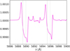 |
Fig. 5 Propagation of RM+CLV model impact for each exposure from Fig. 4 in the final transmission spectrum. The wavelength position of the sodium doublet is indicated as a dotted grey vertical line; the centre of the high-velocity absorption components are indicated as dashed grey vertical lines. The main impact of the RM+CLV correction is at the centre of the sodium doublet, only impacting the mid-centre data and on the blue side of the high-velocity absorption components. |
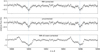 |
Fig. 6 Comparison of sodium doublet with the RM-effect corrected as in Borsa et al. (2021), without corrections, and over-corrected by a factor of five. The line position of the sodium doublet is indicated as a blue dotted line. The corrected doublet is seen on top, the uncorrected doublet in the middle, and the over-correction at the bottom. The high-velocity absorption components cannot be explained by an incorrect RM-effect correction, but are of atmospheric origin as the feature is seen in the uncorrected, corrected, and (even smeared out) in the over-corrected spectra. |
2.4 Impact of stellar or telluric lines
Two other factors that could potentially impact the line shape of the sodium doublet are an insufficient or over-correction of telluric lines, residuals of stellar lines, or telluric sodium emission. We corrected for telluric lines with molecfit (Smette et al. 2015; Kausch et al. 2015), ESO software that takes into account the site conditions at the time of observation. For more details on molecfit, see Allart et al. (2017). We applied the same convergence parameters as described in Seidel et al. (2019) and verified that all telluric lines were corrected down to the noise level in the master spectrum. No residual from the stellar line removal was observed and the S/N remained sufficiently high even at the line core of the stellar sodium doublet so as to not warrant an exclusion of the affected spectra (see Borsa et al. 2019; Seidel et al. 2020a,c, for a discussion on the impact of low S/N stellar residuals). Additionally, in the transmission spectrum as shown e.g. in Fig. 3, no residual from the stellar Ni line at 5892.88 Å is visible. The Earth’s barycentric radial velocity ranged from 11.4 to 11.1 km s−1 during the partial 4-UT transit, with the planetary velocity ranging from −22.7 to 86.1 km s−1. Therefore, residuals of stellar or telluric lines, as well as any impact from the interstellar medium, would be smeared significantly and most likely not show as a concentrated feature. As a consequence, we ruled out these possible sources of the high-velocity absorption component.
Telluric sodium emission is normally monitored on the sky via fibre B of the instrument. However, for the 4-UT-mode transit, fibre B was used for simultaneous wavelength calibration on the Fabry-Perot and no sky observations are available. There are two possible sources of telluric sodium emission: contamination from the laser at UT4 or excitation of atmospheric sodium from meteors. In 4-UT mode, all four UT telescopes of the VLT are used for ESPRESSO, and as a consequence the laser on UT4 is not active, ruling out any laser contamination. The observations took place on 30 Nov. 2018, and no meteor activity was recorded over Chile during that time period. The next meteor shower that could excite the atmosphere sufficiently, the Geminids, did not start before 4 Dec. (peak: 14 Dec). As a consequence, we also ruled out systematic telluric sodium emission as a possible source of the observed feature.
3 Application of MERC
MERC (Seidel et al. 2020b) compares a provided transmission spectrum with a 3D forward model via a nested-sampling retrieval algorithm. The forward model calculates the temperature-pressure profile in 1D and then adds 3D wind patterns and constant planetary rotation assuming tidal locking. The zonal wind patterns can either be constant over the entire atmosphere or scale with solid body rotation with stronger winds at the equator and no winds at the pole (Seidel et al. 2021).
3.1 Implementation of localised jets
We studied a possible atmospheric source for the blueshifted high-velocity absorption components at the sodium doublet. After ruling out a spurious origin of the feature, the high-velocity absorption component likely stems from the blueshift of parts of the sodium population in the atmosphere. The striking features of the high-velocity absorption component are both its distinguishable shape and its clear separation from the main sodium lines hinting at a physically distinct component. A global zonal wind would result in a broad range of velocities visible in the line of sight which would in turn induce a gradual change of the Doppler shift when accounting for the entire atmosphere. As a consequence, the imprint on the transmission spectrum would show a wider range of shifts and a continuous impact on the line shape, for instance as seen for WASP-76 b with its asymmetric line shape encoding both broadening and a blueshifted absorption component from the lower atmosphere (Seidel et al. 2021). Instead of one continuous but deformed line, we see a bimodal distribution of a feature centred at the expected line centre, marking a symmetric distribution of Doppler shifts in the blue and red, and a separate feature at a high velocity range with no connecting intermediate velocity range detected. This is indicative that the particle movement is likely not extending over the entire hemisphere, where it would be strongest at the equator but gradually diminish towards the poles over a wide range of latitudes, but that the moving part of the atmosphere is rather localised in a jet-like stream, leaving us with an imprint of only high velocity Doppler shifts. If the high-velocity absorption components were a consequence of a super-rotational jet that spans the entire atmosphere, it should have a redshifted equivalent from the evening terminator. Each side of the sodium line would have one high-velocity absorption component from the planetary winds aligned with the planetary rotation, creating a symmetric feature around each sodium line. If we consider the second option that can produce strong blue shifts, day-to-night-side winds, we are left with the two cases shown in Fig. 7. Assuming the day-to-night-side wind streams across both terminators equally, on the morning terminator against the planetary rotation and on the evening terminator with the direction of the planetary rotation, we would obtain two high-velocity absorption components (top panel): one at the position of the observed high-velocity absorption component of the egress data and one offset by the differential of the planetary rotation (two times the rotational velocity). If, due to the opening angle of the planet, only one side of the day-to-night side is visible across the terminator, namely the evening terminator, we have the situation of the bottom panel, where only one stream is visible, creating one blueshifted high-velocity absorption component.
That scenario was subsequently implemented in MERC as an additional wind model for the egress data. In the conclusions in Sect. 5, we discuss all different degenerate scenarios that would generate the same imprint on the line shape as discussed above and make the case that a one-sided jet from the day to the night side remains the most likely scenario. To simulate a more locally contained jet, we implemented the day-to-night side wind solely in the latitude range of the tropics and sub-tropics, mimicking observed jets in Solar System planets (Tollefson et al. 2017; Kaspi et al. 2020). In MERC, each atmospheric quadrant is divided in nine atmospheric slices for convergence (for an in-depth explanation of the setup of the model atmosphere see Seidel et al. 2021). We subsequently implemented day-tonight-side winds only in the three slices surrounding the equator, leading to an opening angle of 60° for the jet and keeping its cos θ dependence. Given that a true turning of the model atmosphere to have less of the day-side morning terminator visible during egress is not feasible in the current setup and subsequently is left for future work, we switched off the lower atmospheric wind on the morning terminator, creating a model with one high-velocity absorption component for each sodium doublet line.
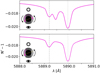 |
Fig. 7 Two models generated with the wind model from MERC for the wavelength range of the sodium D2 line. The position of the sodium line is marked with a dotted grey vertical line. The position of the blueshifted high-velocity absorption components from the egress dataset are marked with a dashed grey vertical line. The lower left corner of each panel shows a sketch of the atmospheric movements. The eye symbolises the observer, the sun the host star, and the black arrows the planetary rotation over each terminator. The scarlet arrows show the direction and existence of atmospheric winds in the lower atmosphere, and the yellow dashed line shows the terminator position to indicate the rotation of the planet with respect to the line of sight for the egress data. |
3.2 Model comparison
For each dataset, the algorithm calculates the Bayesian evidence |In 𝒵| of the current model over the parameter space provided by the priors. The priors used in this work are shown in Table 1. The best-fit parameters are the median of the marginalised posterior distributions. With this approach, different models fitted to the same dataset can be compared by the difference in their Bayesian evidence |ln ℬ01|. We can subsequently judge the significance of the selection of one model over another via the Jeffreys’ scale (see Table 2 or Trotta 2008 and Skilling 2006). The overview of the Jeffreys’ scale, with a more in-depth explanation of its implications and implementation details of MERC, can be found in Seidel et al. (2020b).
4 Retrieval results
We applied MERC to both datasets independently; mid-transit and egress are shown in the top and bottom panels of Fig. 8 in their updated form with planetary rotation and solid body rotation as described in Seidel et al. (2021). The model applied to the egress data only is the jet as described in Sect. 3.1 in the lower atmosphere combined with vertical winds in the upper atmosphere with different altitudes explored for the layer change in this section. The vertical wind is included for the egress dataset based on the results from the mid-transit dataset, which is discussed later in the paper and accounts for the line broadening of the central line component. All the models fed into MERC are the following: an isothermal model with no atmospheric dynamics apart from planetary rotation, a cos θ– dependent day-to-night-side wind (dtncos θ), a cos θ– dependent super-rotational wind (srotcos θ), a vertical wind (ver), and an egress-only model, which is a two layer approach with a jet towards the observer on the evening terminator in the lower atmosphere combined with a vertical wind in the upper atmosphere (dtncos θ, ver).
One of the most powerful tools in Bayesian retrieval is the application of priors. Priors quantify the prior knowledge of the studied problem in boundary conditions. The priors for each of the tested models are listed in Table 1. The prior on the degenerate continuum parameter NaX was left to span various orders of magnitude to allow for a wide range of pressures, given that the pressure and sodium abundance have a significant impact on the broadening. This parameter, which is explained in detail in Seidel et al. (2020b), parametrises the degeneracy between the pressure and the abundance that arises from the loss of the planet’s continuum. This loss of absolute flux value is a result of the processing of high-resolution ground-based data and is explored in more depth in Birkby (2018). The prior of the temperature range is set taking into account the results from Mikal-Evans et al. (2022) spanning from the temperature of the cooler night side to the highest temperature of the temperature inversion.
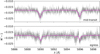 |
Fig. 8 Best fits for both the mid-transit-centred data and the egress data (top and bottom panel, respectively). For the mid-transit data, the best fit is a vertical, radial wind throughout the probed atmosphere; for the egress data, the best fit is achieved with an added jet in the lower atmosphere with cos θ dependence and a vertical wind in the upper atmosphere. The best-fit models are shown in fuchsia on the dataset in grey. |
Overview of the different models’ prior ranges.
Jeffreys’ scale.
4.1 Application to mid-transit data
The calculation of the Bayesian evidence takes model complexity into account. A more complex model with a parameter space of higher dimensionality that converges to the same solution as a more basic model has less Bayesian evidence as a result. This inbuilt characteristic of multi-nested sampling retrieval becomes evident in the application of MERC to the mid-transit data. An inspection of the transmission spectrum shows a surprisingly deep sodium feature that is significantly broadened with no evident net blueshift or redshift and a symmetric line shape. Based on this assessment, we explored four likely scenarios for the line broadening. The most basic model is the isothermal case where the line broadening is solely attributed to temperature and pressure broadening with no atmospheric dynamics. In the three other cases, the isothermal case is combined with either two different types of zonal, horizontal winds or a vertically flowing, radially outwards bound wind. These three types of wind patterns are marked as dtncos θ for the day-to-night-side flow, srotcos θ for the super-rotational flow where the atmosphere rotates faster than the planet itself, and ver for the vertical radial flow. cos θ denotes the solid body type of zonal flow, where the strongest wind speed is located at the equator and no wind is encountered at the poles, mimicking a more physical wind pattern than a homogeneous distribution that creates unphysical artifacts at the poles. For more information on this implementation, see Seidel et al. (2021).
For the mid-transit data, no evidence of either a day-to-night-side wind or a super-rotational jet is found, with the basic model of no winds with a constant temperature profile as the preferred fit. Both the dtncos θ and srotcos θ model converge to wind speeds around 0 and the same temperature range as the basic model. This lead to the conclusion that the difference in evidence is based on the penalisation of more complex models due to the increase in parameters, and, in fact, neither wind pattern has any impact on fit. The vertical wind pattern stands out with strong evidence compared to the other models. For an overview of the Bayesian evidence of each model and their strength of evidence based on the Jeffreys’ scale, we invite the reader to consult Table 3. The posteriors and best fits for all models can be found in Appendix A. The vertical wind has its best fit at a wind speed of 31.3 ± 6.7 km s−1 with a retrieved isothermal temperature of 4093 ± 229 K and the continuum parameter at −2.99 ± 0.07. The large uncertainty most likely stems from the reduced S/N in the dataset due to the split of the transit in a mid-transit and egress dataset. The strong wind speed and high temperature indicated that most likely higher layers of the atmosphere penetrating the lower boundary of the thermosphere are probed. Considering the wide range of altitudes probed, a temperature gradient cannot be ruled out, and the isothermal profile is an approximation instead of the preferred temperature profile. The integration over the terminator, especially during mid-transit, automatically implies that we cannot distinguish between the day- and night-side contribution. The retrieved temperature of ~4100 ± 200 K indicates that lower pressure regimes are probed where the temperature inversion is present (Mikal-Evans et al. 2022). Considering that the dominant wind pattern of radially outwards blowing wind is also attributed to higher atmospheric layers, the driver is higher atmospheric layers.
Additionally, as another intrinsic limitation of transmission spectroscopy from the ground, we lose all information on the probed pressure ranges and operate on relative pressure to an arbitrarily set base pressure only (see for more information Birkby 2018; Seidel et al. 2020b). Considering the wind pattern and the line depth, the assumption that the mid-transit data are able to probe down to our base pressure (the white light radius associated pressure level) is optimistic. It is more likely that the mid-transit dataset probes a lower pressure range higher in the atmosphere, especially considering that the mid-transit dataset probes large parts of the cooler night side where clouds might be present. As a consequence of this pressure uncertainty, the absolute value of the temperature can only be seen as an upper limit set by the line depth from the continuum. A possible way to increase the accuracy of the temperature estimation in the possible presence of clouds is to combine it with low-resolution data to set the lower pressure boundary (e.g. as in Pino et al. 2018) or to use estimations of the relative sodium abundance to break the pressure abundance degeneracy in multi-line studies (e.g. Pino et al. 2018; Allart et al. 2020; Maguire et al. 2023). Both approaches go beyond the scope of this paper and will be left for future work.
Comparison of the different models for the mid-transit data.
Comparison of the different models for the egress data.
4.2 Application to egress data
For the egress data, we chose the same models and priors as for the mid-transit data and added one model with an equatorial jet over the evening terminator as described in Sect. 3.1. The Bayesian evidence derived with MERC is shown in Table 4, and the posteriors for each model together with the best fit can be found in Appendix B. The egress data, together with the best-fit model, is shown in the bottom panel of Fig. 8. Just as for the mid-transit-centred data, both a super-rotational wind and a day-to-night-side wind over both terminators and at all altitudes do not provide a good fit to the data. Due to their higher level of complexity, the isothermal basic model is preferred with moderate evidence. The main peak of the sodium doublet remains broadened compared to the instrument’s profile, which is reflected in the strong evidence for the vertical radial wind model and the best fit for the vertical radial wind model at high velocities instead of close to zero for both the case of only radial winds and the model including a jet-like feature.
To account for the high-velocity absorption components on the blueshifted side, we created a two-layer model with a one-sided jet in the lower atmosphere and vertical radial wind for the central broadening in the upper atmosphere. We based this strategy on two arguments: from global circulation models (GCMs), we know that jets are usually restricted to bands along the equator (Showman et al. 2009, 2018; Parmentier et al. 2018), and from previous work on WASP-76 b, an ultra-hot Jupiter with many of the same characteristics as WASP-121 b, especially in terms of temperature (West et al. 2016), has a lower atmosphere dominated by day-to-night-side winds across both terminators. However, as we do not have resolved data in latitude, a day-to-night-side wind over a broad latitude range is degenerate with a multi-jet scenario as seen in Jupiter’s atmosphere (Liu & Schneider 2010). This two-layer approach requires a switch between wind patterns at a specific point in the vertical structure of the atmosphere. In Seidel et al. (2020b), it was shown that introducing an additional parameter for this switch is not conducive to a better convergence. In MERC, the atmospheric structure in altitude is implemented via a log-scale decrease in pressure from a pre-defined ‘surface’ where the planetary atmosphere becomes opaque. For consistency with existing literature, this surface pressure at the continuum level of the transmission spectrum is set at 10 bar (e.g. Lecavelier Des Etangs et al. 2008; Agúndez et al. 2014; Line et al. 2014; Pino et al. 2018). For the WASP-121 b equivalent, WASP-76 b (Seidel et al. 2021) explored various different altitudes for the switch in wind patterns (10−3 bar, 10−4 bar, and 10−5 bar). The Bayesian evidence indicated that a switch at 10−3 bar is preferred with strong evidence independently of what zonal winds are applied in the lower atmosphere. This pressure is also the upper boundary explored by GCMs for zonal winds (Showman et al. 2009). As a consequence, we set the change from zonal winds to radial winds at the same pressure level for the two-layer model applied here to the egress data of WASP-121 b.
The model including the one-sided jet is preferred over all other models. The next closest model on the Jeffreys’ scale is the vertical wind without jet with a difference of Bayesian evidence of |ln ℬ01| = 1.06, which corresponds to a better fit probability from adding the jet of over 75% (see Table 2 for more information on the Jeffreys’ scale). MERC compares the data over the entire wavelength range of the sodium doublet, which means that in comparison the high-velocity feature only impacts a rather small part of the overall data than the much larger, broadened, main sodium doublet. It is, therefore, not surprising that the difference between the preferred model with the jet and the model with only the vertical wind is not larger given the dominance of the broadened sodium doublet. The posterior distribution with the best-fit parameters, marked in blue for the preferred model (jet and vertical wind), is shown in Fig. 9. The jet velocity is retrieved at 26.7 km s−1 with a one-sigma uncertainty of ±7.2 km s−1, and the vertical wind velocity in the upper atmosphere at 27.8 km s−1 is retrieved with a one sigma uncertainty of ±9.3 km s−1. The best-fit temperature is 3350 ± 470 K, and the continuum parameter is retrieved at −3.1 ± 0.2. The retrieved temperature is compatible with the results from Mikal-Evans et al. (2022), where the day-side shows lower atmospheric temperatures of up to 4000 K above 10−3 bar. The results from Maguire et al. (2023) with a retrieved temperature of 3450 ± 160 K for the day side also stem from high-resolution ESPRESSO data and show that both retrieval approaches produce the same T-P profile with a remarkable level of consistency in the retrieved temperature.
5 Discussion and conclusions
We reanalysed the partial ESPRESSO 4-UT mode transit observations of the ultra-hot Jupiter WASP-121 b first presented in Borsa et al. (2021) to study the resolved sodium doublet. We show that a prominent, blueshifted, high-velocity absorption component seen for both doublet lines stems only from the egress half of the in-transit data by separating the transit in two distinct datasets, the mid-transit centred, and the egress data. We assessed the two most important impacts on the resolved line shape, Doppler smearing caused by the planetary movement during each exposure and the RM-effect. Following Borsa et al. (2021), we show that the RM- and CLV-effect influences the line shape, but that it cannot account for the blueshifted feature. The effect of the Doppler-smearing is estimated at approximately one resolution element and, therefore, has no impact on the line shape beyond the instrumental limits.
We applied MERC to both datasets (mid-transit centred and egress) and show that the broadening of the mid-transit sodium doublet is best retrieved by a vertical, radial wind in the upper atmosphere at 34 ± 7 km s−1. The large uncertainty is due to the reduced S/N from splitting the partial transit into two parts as well as the accounted Doppler smearing from Sect. 2. For the egress data, the best fit is achieved with a vertical wind at 27.8 ± 9.3 km s−1 above 10−3 bar and a jet below that threshold extending across 60° in latitude on the evening limb with a wind velocity of 26.8 ± 7.3 km s−1. The wind model including the jet is preferred over the model with only the vertical wind albeit with a small difference in Bayesian evidence. The localised but strong jet along the equator displaces enough sodium from the expected location in the transmission spectrum via Doppler shifting to account for the blueshifted high-velocity absorption component we first analysed visually on the resolved lines in Borsa et al. (2021). Unfortunately, the 4-UT data lacks the ingress part of the data, which means it is unclear whether this jet feature only exists on the evening terminator or if it is part of a global day-to-night-side wind.
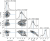 |
Fig. 9 Posterior distribution of isothermal line retrieval with an added jet in the lower atmosphere across the evening terminator and a vertical wind in the upper atmosphere. The change of layers was set at p = 10−3 bar, with the pressure at the surface set to P0 = 10 bar. |
5.1 Constraints on the location of the high-velocity jet
Under the caveat of the difference in Bayesian evidence, in the following we explore the possible location and origin of the jet stream. We plan to observe the ingress of this particular system to further establish the observational evidence and for modelling efforts to include the jet in GCM simulations. The blueshifted high-velocity absorption component is seen for both sodium doublet lines and, at a similar blueshift from line centre, for the H − α line (see Fig. 9 in Borsa et al. 2021). For the resolved K and H − β lines, a similar feature cannot be confirmed due to the noise level (see Figs. 11 and 12 in Borsa et al. 2021). There is no hint of a blueshifted high-velocity absorption component for Li (see Fig. 11 in Borsa et al. 2021); however, all of the mentioned resolved singular lines probing below the altitudes traced by the sodium doublet (Li, K, and H − β) show a pronounced blueshift from the expected line centre. While a rigorous analysis of the blueshift and the similar feature in the H-α line is beyond the scope of this paper and the current capabilities of MERC, the visual inspection allows us to estimate the altitude at which this feature is generated under the strong caveat of a homogeneous continuum level for all these lines. Due to the loss of the planetary continuum (Birkby 2018), this approach can only be seen as a first-order estimate. The 4-UT sodium feature probes up to approximately 1.15 relative planetary radii (Rp), while Li probes only to 1.08 Rp (see Fig. 11 and Table 2 in Borsa et al. 2021). As a consequence, the blueshifted feature is most likely generated at an altitude in the range of [1.08, 1.15] Rp. Under the assumption of a constant base pressure and a hydrostatic atmosphere, this altitude corresponds to the higher layers of the atmosphere above 10−2 bar, which corresponds to the start of the temperature inversion as observed in previous work. The first-order estimate of the origin of the jet is thus compatible with the retrieved temperature regime and we probe the atmosphere in its heated temperature inversion at the base of the thermosphere.
Using the cross-correlation technique on the iron lines to probe deeper layers of the atmosphere, Borsa et al. (2021) estimates that the Fe I lines probe the atmosphere up to 1.05 Rp just below the range we estimate for the origin of the blueshifted high-velocity absorption components. Despite the large uncertainty of the retrieval results of the wind speeds for the jet, the wind speeds probed by the Fe I tracing are below the jet wind speed by a factor of two to three. A possible explanation for this discrepancy is that different, but connected atmospheric layers are probed. The trend for next to no day-to-night-side wind movement for the mid-transit data but a comparatively strong wind in the second half of the data observed for Fe I in Borsa et al. (2021) is also observed for sodium with MERC. However, Fe I only probes up to 1.05 Rp, just below our estimate for the origin of the jet feature at [1.08, 1.15] Rp. This could mean that Fe I probes the lower layers of the jet deeper in the atmosphere, whereas sodium is able to probe the central core of the jet at lower atmospheric density where stronger wind speeds are possible.
Another interesting aspect is the change in visible atmosphere from the mid-transit to the egress data, which is sketched for both the mid-transit and the egress part of the data in Fig. 10. In Sect. 2, we estimate from the orbital phases that the opening angle for the egress data varies from 10° to 30° with a mean opening angle of 20°. Given that no indication of the jet is visible for the mid-transit dataset stretching from −10° to 10°, the jet is most likely starting to be visible across the terminator between an opening angle of 10° to 20° to still generate enough S/N in the integrated transmission spectrum. Both Mikal-Evans et al. (2022) and Daylan et al. (2021) did not observe a significant difference between the brightest and the substellar point from HST observations, as well as in Bourrier et al. (2020b) from TESS observations, indicating that the hotspot, and thus the most likely source of a strong jet stream, is set at the substellar point and not the offset. Additionally, they found a strong temperature difference between the day and night sides, which they attributed to insufficient heat transportation and two distinct realms on the day and night sides. Taking into account these results, it is likely that the jet extends from the substellar point at 90° from the evening terminator to [20, 40]°, after which point it is abruptly dispersed, which is consistent with the HST observations in Evans et al. (2017). This leads us to the conclusion that our observations for the sodium doublet in WASP-121 b are compatible with a supersonic, equatorial jet that is dispersed before it reaches the night side of the atmosphere.
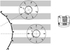 |
Fig. 10 Graphic of atmospheric parts probed during the mid-transit and egress data in a polar planetary view from Fig. 2 updated with the wind patterns. In this polar view, the radial vertical wind is seen in the same way during all in-transit exposures, but the high-velocity jet in the lower atmosphere is only visible during egress. This means its extension cannot reach the evening limb during mid-transit, as it would otherwise also influence the mid-transit data. Given that we have no ingress data, we do not know if the jet is also moving from the day to the night side over the other terminator, is part of a super-rotation, or is not present at all. This missing piece of information is replaced with a question mark. |
5.2 Possible origins of the observed jet and caveats
A similar observation of a high-velocity feature was made from the CCF centroids in Cauley et al. (2021) for the ultra-hot Jupiter WASP-33 b; however, in their analysis they ruled out a supersonic, localised jet as un-physical despite the good fit to their observations. Considering that we constrained the origin of this jet to the upper atmosphere between [1.08, 1.15] Rp, a supersonic jet is far from un-physical. Supersonic jets in planetary atmospheres can be produced by the excitation of a stationary planetary scale Rossby wave by stellar irradiation (Showman & Polvani 2010, 2011), as is likely for tidally locked planets such as WASP-121 b (for an analysis of 3D effects see also Tsai et al. 2014). While these supersonic jets can remain stable across the atmosphere for higher pressures, in the lower pressure regime that is applicable to the here observed jet (P < 10 mbar), supersonic jets are susceptible to large-scale barotropic Kelvin-Helmholtz instabilities and short-scale vertical shear instabilities (Fromang et al. 2016). This scenario is also supported by the results on the temperature structure of the atmosphere.
In this context, it is important to mention a degeneracy in the interpretation of the high-velocity feature as a jet. Due to the opening angle, we probed part of the hotter day side with the evening limb, where we see the origin of the high-velocity feature. However, additionally, we probed more of the night side on the morning limb. A day-to-night-side wind rotates with the planetary rotation on the evening limb, but it provides a Doppler shift against the planetary rotation on the morning limb. In theory, the high-velocity feature could be produced on the night side of the morning limb only or result from a combination of both jets at exactly the correct wind speed difference to offset the planetary rotation. We did not explore these two scenarios further for the following reasons. Assuming that the high-velocity feature is produced by two arms of the jet in both the parts probed on the day side of the evening limb and the night side of the morning limb, the sharpness of the feature with little smearing would mean a near perfect equilibrium between the two components, always offsetting the difference induced by the planetary rotation. The planetary rotation of WASP-121 b is approximately 7.4 km s−1, resulting in a needed offset of ~15 km s−1 for all different contributions over the two limbs at all times and longitudes. While we cannot rule out this coincidental scenario with the current data, it seems unlikely that the night-side jet has velocities ~15 km s−1 larger than the day side. Additionally, if the jet only stems from the probed part of the night side, its velocity would translate to a needed jet velocity of over ~41 ± 7 km s−1 to offset the different LOS velocity of the planetary rotation, which is significantly larger and harder to produce and explain at the probed altitude levels. Additionally, the night side should have a temperature below 2000 K (Mikal-Evans et al. 2022; Bourrier et al. 2020b), while the presented work probes atmospheric layers with temperatures exceeding 3000 K.
For similar results of a day-to-night-side wind for WASP-76 b (Ehrenreich et al. 2020; Kesseli & Snellen 2021; Seidel et al. 2021), the important caveat was raised that a temperature gradient and strong heat transportation across the terminator could create a similar offset (Wardenier et al. 2021). Low-resolution observations over different phases have ruled out this scenario (Evans et al. 2017), showing insufficient heat transportation across the terminator and two distinct regimes on the day and night side. Our hypothesis of a disrupted jet due to instabilities is based on observations of the sodium doublet. It is, in theory, possible that we simply do not trace the super-sonic jet further due to the condensation of sodium. Under the assumption that the jet is visible on the hotter day side, additional ionisation of sodium when crossing to the night side can be ruled out. The condensation scenario, which was proposed for iron in WASP-76 b (Ehrenreich et al. 2020), would require temperatures at approximately 1000 K for half of the atmospheric sodium to condensate to the liquid phase (Wood et al. 2019). Considering night-side temperatures estimated as the lower boundary at 1500 K in the lower atmosphere (Mikal-Evans et al. 2022), it is unlikely that a large fraction of sodium is condensated. While we cannot rule out that our observations trace the temperature gradient and condensation instead of a true disruption due to atmospheric instabilities, it is an unlikely scenario.
Given the high altitudes probed, magnetic drag becomes more significant (Beltz et al. 2022b). Recent work including magneto-hydrodynamics (MHD) in GCMs has shown that magnetic drag can disrupt the often claimed super-rotational jets of ultra-hot Jupiter atmospheres (Beltz et al. 2022b). Given the observational nature of this paper, including MHD is beyond its scope. The application of GCMs including MHD within the observational constraints provided here would allow us to explore the temperature gradient versus Kelvin-Helmholtz instability explanation from first principles, and we encourage such endeavours by other groups.
5.3 Future avenues
Unfortunately, the 4-UT transit is only partial, and we lack the information at ingress to search for the other stream of a possible day-to-night-side jet over both terminators. We therefore cannot say whether the observations show a supersonic, super-rotational jet or one stream of a supersonic day-to-night-side wind. Additionally, we assume that the planet rotates perpendicularly to its orbital plane with the maximum rotational velocity in the line of sight. This is a reasonable assumption given the tidally locked nature of ultra-hot Jupiters, but it will become a major caveat when this technique is applied to smaller exoplanets further out from their host stars.
An important recent avenue to observe atmospheric dynamics in ultra-hot Jupiters is the study of emission lines at various phases, which provides information on the parts of the day-side not accessible during transit (for the first detection of iron in emission see Pino et al. 2020). These emission lines can then be mapped to a likelihood function using the CCF technique and thus give us insights into the line depths and Doppler shifts throughout different phases as first explored in Pino et al. (2022). The time-resolved information of the day side, especially when taking magnetic draft into account (see e.g. Beltz et al. 2022a), provides the information missing from the day side that is not accessible during transit to create a more holistic observational picture of exoplanet atmospheric circulation.
As a future avenue for in-transit observations, we emphasise the need for 4-UT data and several 4-UT transit observations of the same target for a finer phase resolution in resolved line studies. Due to the inherent 3D nature of atmospheres, atmospheric dynamics and thermal or chemical gradients across the terminator can strongly influence the spectral shape. This behaviour can only be recovered by time-resolving transits and by retrieving the evolution of the spectral shape in time. As shown recently for CCF tracing in Gandhi et al. (2022), a time-resolved approach is far superior in fitting the data than 1D time-integrated studies.
The combination of various resolved lines, resolving the issue of varying continuum levels, would allow us to more robustly trace the changes in atmospheric dynamics in transit over a wider range of altitudes than only the line shape and wings of the sodium doublet (see e.g. Zhang et al. 2022). Additionally, the inclusion of various lines will allow the parallel retrieval of relative abundances (see e.g. Gibson et al. 2022; Maguire et al. 2023), which in turn informs a more accurate temperature pressure profile. The study of resolved line shapes will further mature as a tool to study the imprint of atmospheric dynamics as the data quality increases and will unfold its full potential in the era of Extremely Large Telescopes in the next decade.
Acknowledgements
The authors acknowledge the ESPRESSO project team for its effort and dedication in building the ESPRESSO instrument. The ESPRESSO Instrument Project was partially funded through SNSF’s FLARE Programme for large infrastructures. This work relied on observations collected at the European Organisation for Astronomical Research in the Southern Hemisphere. This work has been carried out within the framework of the National Centre of Competence in Research PlanetS supported by the Swiss National Science Foundation. The authors acknowledge the financial support of the SNSF. F.P.E. and C.L.O. would like to acknowledge the Swiss National Science Foundation (SNSF) for supporting research with ESPRESSO through the SNSF grants nr. 140649, 152721, 166227 and 184618. This project has received funding from the European Research Council (ERC) under the European Union’s Horizon 2020 research and innovation programme (project FOUR ACES; grant agreement No 724427) and from the Swiss National Science Foundation for project 200021_200726. It has also been carried out within the framework of the National Centre of Competence in Research PlanetS supported by the Swiss National Science Foundation under grants 51NF40_182901 and 51NF40_205606. Y.A. acknowledges the support of the Swiss National Fund under grant 200020_172746. J.I.G.H., R.R., C.A.P. and A.S.M. acknowledge financial support from the Spanish Ministry of Science and Innovation (MICINN) project PID2020-117493GB-I00. A.S.M., J.I.G.H. and R.R. also acknowledge financial support from the Government of the Canary Islands project ProID2020010129. C.J.M. acknowledges FCT and POCH/FSE (EC) support through Investigador FCT Contract 2021.01214.CEECIND/CP1658/CT0001. R. A. is a Trottier Postdoctoral Fellow and acknowledges support from the Trottier Family Foundation. This work was supported in part through a grant from FRQNT. This work was financed by FCT – Fundação para a Ciência e a Tecnologia under projects UIDB/04434/2020 & UIDP/04434/2020, CERN/FIS-PAR/0037/2019 and PTDC/FIS-AST/0054/2021. The research leading to these results has received funding from the European Research Council (ERC) through the grant agreement 101052347 (FIERCE) and grant agreement 947634 (Spice Dune). This work was supported by FCT – Fundação para a Ciência e a Tecnologia through national funds and by FEDER through COMPETE2020 – Programa Operacional Competitividade e Internacionalização by these grants: UIDB/04434/2020; UIDP/04434/2020. J.L.-B. acknowledges financial support received from “la Caixa” Foundation (ID 100010434) and from the European Unions Horizon 2020 research and innovation programme under the Marie Slodowska-Curie grant agreement No 847648, with fellowship code LCF/BQ/PI20/11760023. This research has also been partly funded by the Spanish State Research Agency (AEI) Project No.PID2019-107061GB-C61. We thank the anonymous referee for their kind comments, which improved the clarity of the main points of the manuscript.
Appendix A Posterior distributions of the retrievals on the mid-transit data
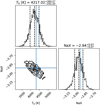 |
Fig. A.1 Posterior distribution of isothermal line retrieval. |
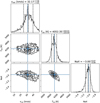 |
Fig. A.2 Posterior distribution of isothermal line retrieval with an added vertical wind constant throughout the atmosphere. |
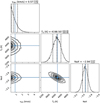 |
Fig. A.3 Posterior distribution of isothermal line retrieval with an added day-to-night-side wind constant throughout the atmosphere. |
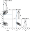 |
Fig. A.4 Posterior distribution of isothermal line retrieval with an added super-rotational wind constant throughout the atmosphere. |
Appendix B Posterior distributions of the retrievals on the egress data
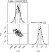 |
Fig. B.1 Posterior distribution of isothermal line retrieval. |
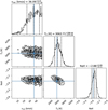 |
Fig. B.2 Posterior distribution of isothermal line retrieval with an added vertical wind constant throughout the atmosphere. |
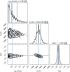 |
Fig. B.3 Posterior distribution of isothermal line retrieval with an added day-to-night-side wind constant throughout the atmosphere. |
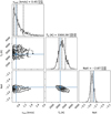 |
Fig. B.4 Posterior distribution of isothermal line retrieval with an added super-rotational wind constant throughout the atmosphere. |
References
- Agúndez, M., Parmentier, V., Venot, O., Hersant, F., & Selsis, F. 2014, A&A, 564, A73 [Google Scholar]
- Allart, R., Lovis, C., Pino, L., et al. 2017, A&A, 606, A144 [NASA ADS] [CrossRef] [EDP Sciences] [Google Scholar]
- Allart, R., Pino, L., Lovis, C., et al. 2020, A&A, 644, A155 [NASA ADS] [CrossRef] [EDP Sciences] [Google Scholar]
- Arcangeli, J., Désert, J.-M., Line, M. R., et al. 2018, ApJ, 855, L30 [Google Scholar]
- Beltz, H., Rauscher, E., Kempton, E. M. R., et al. 2022a, AJ, 164, 140 [NASA ADS] [CrossRef] [Google Scholar]
- Beltz, H., Rauscher, E., Roman, M. T., & Guilliat, A. 2022b, AJ, 163, 35 [NASA ADS] [CrossRef] [Google Scholar]
- Birkby, J. L. 2018, in Handbook of Exoplanets, eds. H.J. Deeg, & J.A. Belmonte (Berlin: Springer), 16 [Google Scholar]
- Borsa, F., & Zannoni, A. 2018, A&A, 617, A134 [NASA ADS] [CrossRef] [EDP Sciences] [Google Scholar]
- Borsa, F., Rainer, M., Bonomo, A. S., et al. 2019, A&A, 631, A34 [NASA ADS] [CrossRef] [EDP Sciences] [Google Scholar]
- Borsa, F., Allart, R., Casasayas-Barris, N., et al. 2021, A&A, 645, A24 [EDP Sciences] [Google Scholar]
- Bourrier, V., Ehrenreich, D., Lendl, M., et al. 2020a, A&A, 635, A205 [NASA ADS] [CrossRef] [EDP Sciences] [Google Scholar]
- Bourrier, V., Kitzmann, D., Kuntzer, T., et al. 2020b, A&A, 637, A36 [NASA ADS] [CrossRef] [EDP Sciences] [Google Scholar]
- Brogi, M., de Kok, R. J., Albrecht, S., et al. 2016, ApJ, 817, 106 [Google Scholar]
- Cabot, S. H. C., Madhusudhan, N., Welbanks, L., Piette, A., & Gandhi, S. 2020, MNRAS, 494, 363 [Google Scholar]
- Casasayas-Barris, N., Palle, E., Stangret, M., et al. 2021, A&A, 647, A26 [NASA ADS] [CrossRef] [EDP Sciences] [Google Scholar]
- Casasayas-Barris, N., Borsa, F., Palle, E., et al. 2022, A&A, 664, A121 [NASA ADS] [CrossRef] [EDP Sciences] [Google Scholar]
- Cauley, P. W., Wang, J., Shkolnik, E. L., et al. 2021, AJ, 161, 152 [Google Scholar]
- Cegla, H. M., Lovis, C., Bourrier, V., et al. 2016, A&A, 588, A127 [NASA ADS] [CrossRef] [EDP Sciences] [Google Scholar]
- Cowan, N. B., Agol, E., & Charbonneau, D. 2007, MNRAS, 379, 641 [NASA ADS] [CrossRef] [Google Scholar]
- Daylan, T., Günther, M. N., Mikal-Evans, T., et al. 2021, AJ, 161, 131 [NASA ADS] [CrossRef] [Google Scholar]
- Delrez, L., Santerne, A., Almenara, J. M., et al. 2016, MNRAS, 458, 4025 [NASA ADS] [CrossRef] [Google Scholar]
- Ehrenreich, D., Lovis, C., Allart, R., et al. 2020, Nature, 580, 597 [Google Scholar]
- Evans, T. M., Sing, D. K., Kataria, T., et al. 2017, Nature, 548, 58 [NASA ADS] [CrossRef] [Google Scholar]
- Fromang, S., Leconte, J., & Heng, K. 2016, A&A, 591, A144 [NASA ADS] [CrossRef] [EDP Sciences] [Google Scholar]
- Gandhi, S., Kesseli, A., Snellen, I., et al. 2022, MNRAS, 515, 749 [NASA ADS] [CrossRef] [Google Scholar]
- Gibson, N. P., Merritt, S., Nugroho, S. K., et al. 2020, MNRAS, 493, 2215 [Google Scholar]
- Gibson, N. P., Nugroho, S. K., Lothringer, J., Maguire, C., & Sing, D. K. 2022, MNRAS, 512, 4618 [NASA ADS] [CrossRef] [Google Scholar]
- Hoeijmakers, H. J., Seidel, J. V., Pino, L., et al. 2020, A&A, 641, A123 [NASA ADS] [CrossRef] [EDP Sciences] [Google Scholar]
- Hoeijmakers, H. J., Kitzmann, D., Morris, B. M., et al. 2022, A&A, submitted [arXiv: 2210.12847] [Google Scholar]
- Kaspi, Y., Galanti, E., Showman, A. P., et al. 2020, Space Sci. Rev., 216, 84 [Google Scholar]
- Kausch, W., Noll, S., Smette, A., et al. 2015, A&A, 576, A78 [NASA ADS] [CrossRef] [EDP Sciences] [Google Scholar]
- Kesseli, A. Y., & Snellen, I. A. G. 2021, ApJ, 908, L17 [Google Scholar]
- Kitzmann, D., Heng, K., Rimmer, P. B., et al. 2018, ApJ, 863, 183 [Google Scholar]
- Knutson, H. A., Charbonneau, D., Allen, L. E., et al. 2007, Nature, 447, 183 [NASA ADS] [CrossRef] [Google Scholar]
- Knutson, H. A., Charbonneau, D., Allen, L. E., Burrows, A., & Megeath, S. T. 2008, ApJ, 673, 526 [Google Scholar]
- Lecavelier Des Etangs, A., Pont, F., Vidal-Madjar, A., & Sing, D. 2008, A&A, 481, L83 [NASA ADS] [CrossRef] [Google Scholar]
- Line, M. R., Fortney, J. J., Marley, M. S., & Sorahana, S. 2014, ApJ, 793, 33 [Google Scholar]
- Liu, J., & Schneider, T. 2010, J. Atmos. Sci., 67, 3652 [NASA ADS] [CrossRef] [Google Scholar]
- Lothringer, J. D., Barman, T., & Koskinen, T. 2018, ApJ, 866, 27 [NASA ADS] [CrossRef] [Google Scholar]
- Louden, T., & Wheatley, P. J. 2015, ApJ, 814, L24 [CrossRef] [Google Scholar]
- Maguire, C., Gibson, N. P., Nugroho, S. K., et al. 2023, MNRAS, 519, 1030 [Google Scholar]
- McLaughlin, D. B. 1924, Popular Astron., 32, 225 [NASA ADS] [Google Scholar]
- Merritt, S. R., Gibson, N. P., Nugroho, S. K., et al. 2021, MNRAS, 506, 3853 [NASA ADS] [CrossRef] [Google Scholar]
- Mikal-Evans, T., Sing, D. K., Barstow, J. K., et al. 2022, Nat. Astron., 6, 471 [NASA ADS] [CrossRef] [Google Scholar]
- Montalto, M., Santos, N. C., Boisse, I., et al. 2011, A&A, 528, L17 [NASA ADS] [CrossRef] [EDP Sciences] [Google Scholar]
- Mounzer, D., Lovis, C., Seidel, J. V., et al. 2022, A&A, 668, A1 [NASA ADS] [CrossRef] [EDP Sciences] [Google Scholar]
- Parmentier, V., Line, M. R., Bean, J. L., et al. 2018, A&A, 617, A110 [NASA ADS] [CrossRef] [EDP Sciences] [Google Scholar]
- Pepe, F., Cristiani, S., Rebolo, R., et al. 2021, A&A, 645, A96 [NASA ADS] [CrossRef] [EDP Sciences] [Google Scholar]
- Pino, L., Ehrenreich, D., Wyttenbach, A., et al. 2018, A&A, 612, A53 [NASA ADS] [CrossRef] [EDP Sciences] [Google Scholar]
- Pino, L., Désert, J.-M., Brogi, M., et al. 2020, ApJ, 894, L27 [Google Scholar]
- Pino, L., Brogi, M., Désert, J. M., et al. 2022, A&A, 668, A176 [NASA ADS] [CrossRef] [EDP Sciences] [Google Scholar]
- Ridden-Harper, A. R., Snellen, I. A. G., Keller, C. U., et al. 2016, A&A, 593, A129 [NASA ADS] [CrossRef] [EDP Sciences] [Google Scholar]
- Rossiter, R. A. 1924, ApJ, 60, 15 [Google Scholar]
- Sedaghati, E., MacDonald, R. J., Casasayas-Barris, N., et al. 2021, MNRAS, 505, 435 [NASA ADS] [CrossRef] [Google Scholar]
- Seidel, J. V., Ehrenreich, D., Wyttenbach, A., et al. 2019, A&A, 623, A166 [NASA ADS] [CrossRef] [EDP Sciences] [Google Scholar]
- Seidel, J. V., Ehrenreich, D., Bourrier, V., et al. 2020a, A&A, 641, L7 [NASA ADS] [CrossRef] [EDP Sciences] [Google Scholar]
- Seidel, J. V., Ehrenreich, D., Pino, L., et al. 2020b, A&A, 633, A86 [NASA ADS] [CrossRef] [EDP Sciences] [Google Scholar]
- Seidel, J. V., Lendl, M., Bourrier, V., et al. 2020c, A&A, 643, A45 [NASA ADS] [CrossRef] [EDP Sciences] [Google Scholar]
- Seidel, J. V., Ehrenreich, D., Allart, R., et al. 2021, A&A, 653, A73 [NASA ADS] [CrossRef] [EDP Sciences] [Google Scholar]
- Seidel, J. V., Cegla, H. M., Doyle, L., et al. 2022, MNRAS, 513, L15 [NASA ADS] [CrossRef] [Google Scholar]
- Showman, A. P., & Polvani, L. M. 2010, Geophys. Res. Lett., 37, L18811 [Google Scholar]
- Showman, A. P., & Polvani, L. M. 2011, ApJ, 738, 71 [Google Scholar]
- Showman, A. P., Fortney, J. J., Lian, Y., et al. 2009, ApJ, 699, 564 [NASA ADS] [CrossRef] [Google Scholar]
- Showman, A. P., Tan, X., & Zhang, X. 2018, AGU Fall Meeting Abstracts, P43E-3818 [Google Scholar]
- Skilling, J. 2006, Bayesian Anal., 1, 833 [Google Scholar]
- Smette, A., Sana, H., Noll, S., et al. 2015, A&A, 576, A77 [NASA ADS] [CrossRef] [EDP Sciences] [Google Scholar]
- Smith, B. A., Soderblom, L. A., Johnson, T. V., et al. 1979, Science, 204, 951 [NASA ADS] [CrossRef] [Google Scholar]
- Snellen, I. A. G., de Kok, R. J., de Mooij, E. J. W., & Albrecht, S. 2010, Nature, 465, 1049 [Google Scholar]
- Tabernero, H. M., Zapatero Osorio, M. R., Allart, R., et al. 2021, A&A, 646, A158 [NASA ADS] [CrossRef] [EDP Sciences] [Google Scholar]
- Tollefson, J., Wong, M. H., Pater, I.D., et al. 2017, Icarus, 296, 163 [NASA ADS] [CrossRef] [Google Scholar]
- Trotta, R. 2008, Contemp. Phys., 49, 71 [Google Scholar]
- Tsai, S.-M., Dobbs-Dixon, I., & Gu, P.-G. 2014, ApJ, 793, 141 [NASA ADS] [CrossRef] [Google Scholar]
- Wardenier, J. P., Parmentier, V., Lee, E. K. H., Line, M. R., & Gharib-Nezhad, E. 2021, MNRAS, 506, 1258 [NASA ADS] [CrossRef] [Google Scholar]
- Wardenier, J. P., Parmentier, V., & Lee, E. K. H. 2022, MNRAS, 510, 620 [Google Scholar]
- West, R. G., Hellier, C., Almenara, J. M., et al. 2016, A&A, 585, A126 [NASA ADS] [CrossRef] [EDP Sciences] [Google Scholar]
- Wilson, J., Gibson, N. P., Lothringer, J. D., et al. 2021, MNRAS, 503, 4787 [NASA ADS] [CrossRef] [Google Scholar]
- Wood, B. J., Smythe, D. J., & Harrison, T. 2019, Am. Mineral., 104, 844 [NASA ADS] [CrossRef] [Google Scholar]
- Wyttenbach, A., Ehrenreich, D., Lovis, C., Udry, S., & Pepe, F. 2015, A&A, 577, A62 [NASA ADS] [CrossRef] [EDP Sciences] [Google Scholar]
- Wyttenbach, A., Mollière, P., Ehrenreich, D., et al. 2020, A&A, 638, A87 [EDP Sciences] [Google Scholar]
- Yan, F., Pallé, E., Fosbury, R. A. E., Petr-Gotzens, M. G., & Henning, T. 2017, A&A, 603, A73 [NASA ADS] [CrossRef] [EDP Sciences] [Google Scholar]
- Zhang, Y., Snellen, I.A.G., Wyttenbach, A., et al. 2022, A&A, 666, A47 [NASA ADS] [CrossRef] [EDP Sciences] [Google Scholar]
All Tables
All Figures
|
Fig. 1 Graphic of data taken and the split into two datasets for the 4-UT ESPRESSO transit. Time is indicated as phase on the x-axis, with the planetary orbit marked as a dashed arrow indicating the direction of movement in time across the stellar disc. The grey areas indicate when exposures where obtained during transit and how the data was split into one set centred around mid-transit (0.0, darker grey, mid-transit dataset) and the other comprising the rest of the exposures towards egress (from here called the egress dataset). |
| In the text | |
|
Fig. 2 Graphic of atmospheric parts probed during the separated parts of mid-transit and egress data in a polar planetary view. The host star is indicated on the left, with the observer as a small VLT UT on the right. WASP-121 b is shown in the middle with its obscure planet disc as the smaller circle and the atmosphere extension as the larger circle. The grey areas indicate the light from the host star crossing the exo-planet atmosphere over each limb in the line of sight. The depiction of WASP-121 b at the bottom is shown roughly at mid-transit, where the terminator (short dashed line) is orthogonal to the line of sight. At the top it is shown at a moment in time during the egress part of the dataset, when the planet has rotated and shows a different opening angle than during mid-transit, with different parts of the atmosphere probed across both limbs. The opening angle is indicated by the longer, dashed lines starting at the centre of the host star. The graphic is not to scale. |
| In the text | |
|
Fig. 3 Sodium doublet transmission spectra for the partial 4-UT transit normalised to zero. The top panel shows the full dataset combined, in agreement down to the noise level with Borsa et al. (2021), the central panel shows the mid-transit-centred dataset, and the bottom panel gives the egress-centred dataset. The line centre of the sodium doublet lines are indicated as dotted, blue, vertical lines. The egress data shows a distinct high-velocity absorption feature on the blue side of each sodium doublet line, which is the feature under investigation in this work. The position of this feature is highlighted in each of the three panels by the light blue dashed line. |
| In the text | |
|
Fig. 4 RM+CLV model from Borsa et al. (2021) as a function of phase in the planetary rest frame. The start of the transit is at the bottom; time moves vertically and is emphasised by the colour gradient. The end of the transit is indicated with a dashed, grey horizontal line. The wavelength position of the sodium doublet is indicated as dotted grey vertical lines; the centre of the high-velocity absorption components are indicated as dashed grey vertical lines. |
| In the text | |
|
Fig. 5 Propagation of RM+CLV model impact for each exposure from Fig. 4 in the final transmission spectrum. The wavelength position of the sodium doublet is indicated as a dotted grey vertical line; the centre of the high-velocity absorption components are indicated as dashed grey vertical lines. The main impact of the RM+CLV correction is at the centre of the sodium doublet, only impacting the mid-centre data and on the blue side of the high-velocity absorption components. |
| In the text | |
|
Fig. 6 Comparison of sodium doublet with the RM-effect corrected as in Borsa et al. (2021), without corrections, and over-corrected by a factor of five. The line position of the sodium doublet is indicated as a blue dotted line. The corrected doublet is seen on top, the uncorrected doublet in the middle, and the over-correction at the bottom. The high-velocity absorption components cannot be explained by an incorrect RM-effect correction, but are of atmospheric origin as the feature is seen in the uncorrected, corrected, and (even smeared out) in the over-corrected spectra. |
| In the text | |
|
Fig. 7 Two models generated with the wind model from MERC for the wavelength range of the sodium D2 line. The position of the sodium line is marked with a dotted grey vertical line. The position of the blueshifted high-velocity absorption components from the egress dataset are marked with a dashed grey vertical line. The lower left corner of each panel shows a sketch of the atmospheric movements. The eye symbolises the observer, the sun the host star, and the black arrows the planetary rotation over each terminator. The scarlet arrows show the direction and existence of atmospheric winds in the lower atmosphere, and the yellow dashed line shows the terminator position to indicate the rotation of the planet with respect to the line of sight for the egress data. |
| In the text | |
|
Fig. 8 Best fits for both the mid-transit-centred data and the egress data (top and bottom panel, respectively). For the mid-transit data, the best fit is a vertical, radial wind throughout the probed atmosphere; for the egress data, the best fit is achieved with an added jet in the lower atmosphere with cos θ dependence and a vertical wind in the upper atmosphere. The best-fit models are shown in fuchsia on the dataset in grey. |
| In the text | |
|
Fig. 9 Posterior distribution of isothermal line retrieval with an added jet in the lower atmosphere across the evening terminator and a vertical wind in the upper atmosphere. The change of layers was set at p = 10−3 bar, with the pressure at the surface set to P0 = 10 bar. |
| In the text | |
|
Fig. 10 Graphic of atmospheric parts probed during the mid-transit and egress data in a polar planetary view from Fig. 2 updated with the wind patterns. In this polar view, the radial vertical wind is seen in the same way during all in-transit exposures, but the high-velocity jet in the lower atmosphere is only visible during egress. This means its extension cannot reach the evening limb during mid-transit, as it would otherwise also influence the mid-transit data. Given that we have no ingress data, we do not know if the jet is also moving from the day to the night side over the other terminator, is part of a super-rotation, or is not present at all. This missing piece of information is replaced with a question mark. |
| In the text | |
|
Fig. A.1 Posterior distribution of isothermal line retrieval. |
| In the text | |
|
Fig. A.2 Posterior distribution of isothermal line retrieval with an added vertical wind constant throughout the atmosphere. |
| In the text | |
|
Fig. A.3 Posterior distribution of isothermal line retrieval with an added day-to-night-side wind constant throughout the atmosphere. |
| In the text | |
|
Fig. A.4 Posterior distribution of isothermal line retrieval with an added super-rotational wind constant throughout the atmosphere. |
| In the text | |
|
Fig. B.1 Posterior distribution of isothermal line retrieval. |
| In the text | |
|
Fig. B.2 Posterior distribution of isothermal line retrieval with an added vertical wind constant throughout the atmosphere. |
| In the text | |
|
Fig. B.3 Posterior distribution of isothermal line retrieval with an added day-to-night-side wind constant throughout the atmosphere. |
| In the text | |
|
Fig. B.4 Posterior distribution of isothermal line retrieval with an added super-rotational wind constant throughout the atmosphere. |
| In the text | |
Current usage metrics show cumulative count of Article Views (full-text article views including HTML views, PDF and ePub downloads, according to the available data) and Abstracts Views on Vision4Press platform.
Data correspond to usage on the plateform after 2015. The current usage metrics is available 48-96 hours after online publication and is updated daily on week days.
Initial download of the metrics may take a while.