| Issue |
A&A
Volume 653, September 2021
|
|
|---|---|---|
| Article Number | A104 | |
| Number of page(s) | 17 | |
| Section | Planets and planetary systems | |
| DOI | https://doi.org/10.1051/0004-6361/202140559 | |
| Published online | 14 September 2021 | |
The GAPS Programme at TNG
XXXI. The WASP-33 system revisited with HARPS-N★
1
INAF – Osservatorio Astronomico di Brera,
Via E. Bianchi 46,
23807
Merate (LC),
Italy
e-mail: francesco.borsa@inaf.it
2
INAF – Osservatorio Astrofisico di Catania,
Via S. Sofia 78,
95123
Catania,
Italy
3
Dipartimento di Fisica, Università degli Studi di Milano Bicocca,
Piazza dell’Ateneo Nuovo, 1,
20126
Milano,
Italy
4
INAF – Osservatorio Astrofisico di Arcetri,
Largo E. Fermi 5,
50125
Firenze,
Italy
5
Space Research Institute, Austrian Academy of Sciences,
Schmiedlstrasse 6,
8042
Graz,
Austria
6
Department of Physics, University of Warwick,
Coventry
CV4 7AL,
UK
7
INAF – Osservatorio Astrofisico di Torino,
Via Osservatorio 20,
10025,
Pino Torinese,
Italy
8
Centre for Exoplanets and Habitability, University of Warwick,
Gibbet Hill Road,
Coventry
CV4 7AL,
UK
9
INAF-IAPS Istituto di Astrofisica e Planetologia Spaziali,
Via del Fosso del Cavaliere 100,
00133,
Roma,
Italy
10
INAF – Osservatorio Astronomico di Padova,
Vicolo dell’Osservatorio 5,
35122,
Padova,
Italy
11
INAF – Osservatorio Astronomico di Palermo,
Piazza del Parlamento, 1,
90134,
Palermo,
Italy
12
INAF – Osservatorio Astronomico di Trieste,
via Tiepolo 11,
34143
Trieste,
Italy
13
Thüringer Landessternwarte Tautenburg,
Sternwarte 5,
07778,
Tautenburg,
Germany
14
Department of Physics, University of Rome Tor Vergata,
Via della Ricerca Scientifica 1,
00133
Rome,
Italy
15
Max Planck Institute for Astronomy,
Königstuhl 17,
69117,
Heidelberg,
Germany
16
Fundación Galileo Galilei - INAF,
Rambla José Ana Fernandez Pérez 7,
38712
Breña Baja,
TF,
Spain
17
Instituto de Astrofísica de Canarias (IAC),
C/Vía Láctea s/n,
38205
La Laguna,
TF,
Spain
18
Departamento de Astrofísica, Universidad de La Laguna (ULL),
38206
La Laguna,
TF,
Spain
19
INAF – Osservatorio Astronomico di Capodimonte,
Salita Moiariello 16,
80131,
Napoli,
Italy
20
INAF – Osservatorio di Cagliari,
via della Scienza 5,
09047
Selargius,
CA,
Italy
21
Dip. di Fisica e Astronomia Galileo Galilei – Università di Padova,
Vicolo dell’Osservatorio 2,
35122
Padova,
Italy
Received:
14
February
2021
Accepted:
21
May
2021
Context. Giant planets in short-period orbits around bright stars represent optimal candidates for atmospheric and dynamical studies of exoplanetary systems.
Aims. We aim to analyse four transits of WASP-33b observed with the optical high-resolution HARPS-N spectrograph to confirm its nodal precession, study its atmosphere, and investigate the presence of star-planet interactions.
Methods. We extracted the mean line profiles of the spectra using the least-squares deconvolution method, and we analysed the Doppler shadow and the radial velocities. We also derived the transmission spectrum of the planet, correcting it for the stellar contamination due to rotation, centre-to-limb variations, and pulsations.
Results. We confirm the previously discovered nodal precession of WASP-33b, almost doubling the time coverage of the inclination and projected spin-orbit angle variation. We find that the projected obliquity reached a minimum in 2011, and we used this constraint to derive the geometry of the system, and in particular its obliquity at that epoch (ϵ = 113.99° ± 0.22°) and the inclination of the stellar spin axis (is = 90.11° ± 0.12°). We also derived the gravitational quadrupole moment of the star J2 = (6.73 ± 0.22) × 10−5, which we find to be in close agreement with the theoretically predicted value. Small systematics errors are computed by shifting the date of the minimum projected obliquity. We present detections of Hα and Hβ absorption in the atmosphere of the planet, with a contrast almost twice as small as that previously detected in the literature. We also find evidence for the presence of a pre-transit signal, which repeats in all four analysed transits and should thus be related to the planet. The most likely explanation lies in a possible excitation of a stellar pulsation mode by the presence of the planetary companion.
Conclusions. A future common analysis of all available datasets in the literature will help shed light on the possibility that the observed Balmer lines’ transit depth variations are related to stellar activity and pulsation, and to set constraints on the planetary temperature–pressure structure and thus on the energetics possibly driving atmospheric escape. A complete orbital phase coverage of WASP-33b with high-resolution spectroscopic (and spectro-polarimetric) observations could help us to understand the nature of the pre-transit signal.
Key words: techniques: spectroscopic / planetary systems / planets and satellites: atmospheres / stars: individual: WASP-33 / techniques: radial velocities
Based on observations made with the Italian Telescopio Nazionale Galileo (TNG) operated on the island of La Palma by the Fundacion Galileo Galilei of the INAF at the Spanish Observatorio Roque de los Muchachos of the IAC in the frame of the program Global Architecture of the Planetary Systems (GAPS).
© ESO 2021
1 Introduction
Transiting exoplanets orbiting intermediate-mass (e.g. A-type) stars on short-period (Porb≤5 days) orbits are excellentlaboratories for atmospheric and dynamical studies. The high day-side equilibrium temperatures of these ultra-hot Jupiters (UHJs, Teq ≥ 2200 K) cause the thermal dissociation of most molecules (e.g. Lothringer et al. 2018; Arcangeli et al. 2018). Depending on the heat transfer efficiency in the atmosphere, there might also be variations in the chemical composition of the day-side, night-side and terminator of the planet (e.g., Parmentier et al. 2018). Orbiting at short distances from their parent star, the strong stellar ultraviolet irradiation makes the planetary atmosphere undergo a significant mass loss, affecting its composition and evolution (e.g. Fossati et al. 2018a).
Short-period systems are also interesting because they experience strong tidal interactions between the planet and its host star. Star-planet tidal interactions could modify the stellar rotation rate along the system’s evolution (Gallet et al. 2018), cause planet oblateness (Akinsanmi et al. 2019), suppress stellar activity (Fossati et al. 2018b), and induce stellar pulsations (de Wit et al. 2017). The measure of the projected spin-orbit angle either with radial velocities (RVs) through the Rossiter-McLaughlin effect (RM, Rossiter 1924; McLaughlin 1924), or with the Doppler tomography technique (e.g. Collier Cameron et al. 2010a) can help to shed light on a system evolution history (e.g. Fabrycky & Winn 2009).
In this context, WASP-33b (Collier Cameron et al. 2010b) is a very intriguing target. It is a UHJ (Mp ~ 2.2 MJup, Rp ~ 1.6 RJup) orbiting in ~1.21 days a bright δ-Scuti A-type star (V = 8.3, Teff ~ 7500 K, v sin is ~ 86 km s−1) with a highly misaligned projected spin–orbit angle: λ ~ −110 degrees (Collier Cameron et al. 2010b; Lehmann et al. 2015). Stellar non-radial pulsations were already noted spectroscopically in the discovery paper (Collier Cameron et al. 2010b). Photometric oscillations of the star were first reported by Herrero et al. (2011), and the stellar pulsation spectrum has been analysed in different studies (Kovács et al. 2013; von Essen et al. 2014; Mkrtichian 2015; von Essen et al. 2020). Because of its easily detected stellar pulsations, the WASP-33 system has been considered a good candidate for the detection of star-planet interactions (Herrero et al. 2011). WASP-33b was also noted as a possible target for which both classical and relativistic node precessional effects could be evidenced within a reasonable amount of time (Iorio 2011, 2016); indeed, classical node precessional effects were subsequently detected by Johnson et al. (2015) and Watanabe et al. (2020).
Its atmosphere has also been the subject of different studies. The probable presence of a temperature inversion in its atmosphere (Haynes et al. 2015; von Essen et al. 2015) was best explained by the presence of titanium oxide (TiO); however the detection of TiO using high-resolution spectroscopy is debated (Nugroho et al. 2017; Herman et al. 2020). Other results include the first indication of aluminum oxide (AlO) in an exoplanet using low-resolution spectrophotometry (von Essen et al. 2019), the detection of ionised calcium (Ca II H&K) up to very high upper-atmosphere layers close to the planetary Roche lobe (Yan et al. 2019), and the detection of Balmer lines (Yan et al. 2021; Cauley et al. 2021). The existence of a thermal inversion was recently confirmed with the detection of Fe I in emission using high-resolution observations (Nugroho et al. 2020).
Driven by the intriguing characteristics of the system, in this work we analysed new transits of WASP-33b taken with the HARPS-N high-resolution spectrograph, looking for confirmation of the nodal precession and exploring its atmosphere. This manuscript is organised as follows. We first present our data in Sect. 2, then analyse the planetary Doppler shadow and the in-transit RVs also studying the precession of the orbital plane and the spin of the host star (Sects. 3 and 4). We studied the planetary atmosphere focusing on Hα and Hβ absorption in Sect. 5, finding a pre-transit signal coherent with the planetary orbital period discussed in Sect. 6. Then, we looked for other atmospheric species with the cross-correlation technique described in Sect. 7. We end with our summary and conclusions in Sect. 8.
2 Data sample
We observed WASP-33 during four transits using the high-resolution (resolving power R ~ 115 000) HARPS-N spectrograph (Cosentino et al. 2012) mounted at the Telescopio Nazionale Galileo on La Palma island and covering the 380–690 nm wavelength range. The first two transits were observed with HARPS-N only (program A34TAC42, PI Nascimbeni), while the other two were taken in the framework of the GAPS project (Covino et al. 2013). The latter were observed using the GIARPS configuration (Claudi et al. 2017), but in this manuscript we focus only on the HARPS-N data.
The transit of WASP-33b lasts 2 h48 min. Three transit observations were monitored with exposures of 600 s, while for one we used a longer cadence (900 s exposure). While fiber A of the spectrograph was centred on the target, for all the transits fiber B was simultaneously monitoring the sky to check for possible atmospheric emission contamination. The log of the observations is reported in Table 1.
The quality of transit two rapidly decreases after the transit ingress due to weather conditions, we thus decided to not include it in the analysis of the transmission spectrum, Doppler shadow, and RVs, but we do include it in Sect. 6, where we look at the pre-transit portion of the data.
WASP-33 HARPS-N observations log.
3 Precession of the orbital plane and stellar spin axis
WASP-33 is a δ-Sct A-type star. Since no default A-type mask is supported by the HARPS-N DRS pipeline (Cosentino et al. 2014), we followed the approach presented in Borsa et al. (2019) and extracted the mean line profiles using the least-squares deconvolution (LSD) software (Donati et al. 1997). This software performs a least-squares deconvolution of the normalised spectra with a theoretical line mask extracted from the Vienna Atomic Line Database (VALD, Piskunov et al. 1995). We used a stellar mask with Teff = 7500 K, log g = 4.0, and solar metallicity. We accurately re-normalised the spectra (order-by-order by using polynomials; see Rainer et al. (2016) for a detailed description of the procedure) and converted them to the required format, working only on the wavelength regions 441.5–480.5 nm, 491.5–528.5 nm, 536.5–587.0 nm, 605.0–626.5 nm, and 633.5–645.0 nm, hence cutting the blue orders where the signal-to-noise ratio (S/N) was very low due to the instrument efficiency, the Balmer lines, and the regions where most of the telluric lines are found. We then created mean line profile residuals by dividing all the mean line profiles by amaster out-of-transit mean line profile for each transit observed. As already evidenced by Collier Cameron et al. (2010b) and Johnson et al. (2015), the Doppler shadow of the planet is clearly visible as well as the stellar pulsations (Fig. 1, left panel). We note that the pulsations are more evident on the edge of the lines with respect to the centre, which is a hint of non-radial pulsations (see also Collier Cameron et al. 2010b).
For planets with projected spin-orbit angles close to 90°, nodal precession can be more easily detected during observations spanning several years (Watanabe et al. 2020). WASP-33b is one of the two reported cases where the exoplanet orbit has been found to show nodal precession (Johnson et al. 2015; Watanabe et al. 2020), with the other case being Kepler-13Ab (Szabó et al. 2012; Herman et al. 2018). Since our dataset extends the timespan of the reported orbital variations, we tried to see if this was also visible in our data. We removed stellar pulsations independently for each single transit using Fourier transform filtering (Fig. 1) following the method presented in Johnson et al. (2015). This exploits the fact that pulsations (prograde) and Doppler shadow (retrograde) propagate in opposite directions: their frequency components thus tend to be separated in the two-dimensional Fourier transform of the line profile residuals’ time series (Johnson et al. 2015). We then performed a fit to the Doppler shadow. The Doppler shadow model is taken from EXOFASTv2 (Eastman 2017; Eastman et al. 2019), passed through the Fourier filter, and fitted to the data in a Bayesian framework by employing a differential evolution Markov chain Monte Carlo (DE-MCMC) technique (Ter Braak 2006; Eastman et al. 2013), running five DE-MCMC chains of 100,000 steps and discarding the burn-in. We fixed v sin is, a∕Rs, T0, period, Rp /Rs to the values of Table 2. We left the projected spin-orbit angle λ and the inclination angle i, for which we set uninformative priors, as free parameters. The medians and the 15.86% and 84.14% quantiles of the posterior distributions were taken as the best values and 1σ uncertainties.
Our results (Fig. 2, Table 2), together with the previous measurements of Watanabe et al. (2020), confirm the precession of the planetary orbit and that the obliquity projected on the plane of the sky λ reached a minimum in 2011. This allows us to determine the inclination of the stellar spin axis to the line of sight is and the obliquity ϵ at the epoch when dλ∕dt = 0, thus allowing a more precise description of the precession of the system and the measure of the stellar gravitational quadrupole moment J2. We describe the method applied to determine the system geometry as well as the rate of precession of the nodes of the orbital plane in Appendix A.
The rate of change of the inclination angle of the orbital plane i can be regarded as constant over the time span of the observations (~ 10 yr) because it is much shorter than the precession period (~1100 yr; see below). It is measured by a weighted linear best fit to the data in Fig. 2 (upper panel), giving d i∕d t = 0.324 ± 0.006 deg yr−1, while the epoch when dλ∕dt = 0 is assumed to coincide with the transit observed on 19 October 2011, when i = 87.56° ± 0.037° and λ = − 114.01° ± 0.22° (Watanabe et al. 2020). Given the uncertainty on such an epoch, we report the systematic deviations in the derived model parameters corresponding to a shift of the epoch of dλ∕dt = 0 by ± 500 days since the assumed epoch, respectively (Table A.1). To compute these deviations, we assume that d i∕d t has the same value as above, while we linearly interpolated for the parameter i and cubicly interpolated for the parameter λ to find their values at the two epochs. For each parameter, we report the standard deviation as a measure of the statistical error, while in brackets we add the systematic deviation when d λ∕d t = 0 at the later epoch and the deviation when dλ∕dt = 0 at the earlier epoch, respectively. We note that the two deviations have the same sign when the parameter reached an extremum in between the considered epoches.
Following the method described in Appendix A, we find that the stellar spin is perpendicular to the line of sight (is = 90.11° ± 0.12° (−0.026°;−0.015°)), while the obliquity ϵ = 113.99° ± 0.22° (−0.24°;−0.67°) at the epoch of the transit on 19 October 2011. From the spectroscopic stellar v sin is, is, and stellar radius, we estimate a rotation period of thestar of 0.884 ± 0.02 days, not significantly affected by the systematic errors on is because it is close to 90°. The precession rate of the nodes of the orbital plane is found to be − 0.325 ± 0.006 (6.7 × 10⁻⁵;1.1 × 10⁻⁴) deg yr−1, giving a precession period of 1108 ± 19 (0.23;0.38) yr, slightly longer than that determined by Johnson et al. (2015). The time interval during which transits by WASP-33b are observable is thus of ~97 yr, centred around 2019, which is slightly longer than their interval of about ~ 88 yr.
Our inclination is of the stellar spin axis to the line of sight is different from the value found by Iorio (2016) because his determination was based on the parameters derived only from the transits of 2008 and 2014 as reported by Johnson et al. (2015). This led Iorio to consider a constant precession rate of the angle I of his model, while our more extended dataset shows that dI∕dt is variable and became zero around 2011. In Appendix A.5, we account for the differences between his results and ours and show how the application of his model to our dataset reproduces our value of is and of the stellar quadrupole moment (see below).
Previous analyses of the precession of WASP-33b by Johnson et al. (2015) and Watanabe et al. (2020) assumed that the stellar spin angular momentum is much larger than the orbital angular momentum because they adopted the gyration radius γ typical of a Sun-like star following the exploratory calculations by Iorio (2011). Here, we determine more appropriate values of the gyration radius and apsidal motion constant k2 of WASP-33 by making use of the tabulations of Claret (2019). Considering the uncertainties in the stellar mass and effective temperature, we find that Claret’s model with solar metallicity and mass of 1.6 M⊙ is adequate to describe WASP-33. Taking into account the correction for its fast rotation, we find log k2 = −2.55 ± 0.014 and γ = 0.1884 ± 0.0019, where the uncertainties only take into account the uncertainty in the stellar effective temperature.
With the above values of k2, γ, and the adopted stellar and planetary parameters, we predict a value of d i∕dt = 0.315 ± 0.026 (0.0023;0.0068) deg yr−1 and a precession rate of the nodes of − 0.316 ± 0.026 (0.0024;0.0069) deg yr−1 using the formulae given in Appendix A.3. The coincidence of these numerical values comes from the geometry of the system as explained there. These precession rates differ by less than a half standard deviation from the observed ones, supporting the correctness of the adopted stellar parameters. With our value of γ and the adopted system parameters, we find that the ratio of the stellar spin to the orbital angular momentum is 2.75 ± 0.33, therefore we cannot neglect the precession of the stellar spin. It occurs within the same period as the precession of the node of the orbital plane and makes the inclination is of the stellar spin axis to the line of sight vary between 67.5° and 110.8° along a complete precession cycle. We note that an inclination of the stellar spin greater than 90° implies that the south pole of the star is in view, so the apparent stellar rotation is clockwise, contrary to the usual anticlockwise rotation assumed when is < 90° and the north pole is in view.
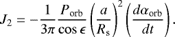
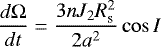
The fast stellar rotation produces a deformation in the stellar mass distribution and hence a distortion in the gravitational field. The stellar gravitational quadrupole moment J2 can be deduced from the observed nodal precession rate of the orbital plane according to Eq. (3) of Johnson et al. (2015) and is (6.73 ± 0.22 [0.062;0.18]) × 10−5. This value compares well with the theoretically expected value of (6.53 ± 0.41 [0.011;0.031]) × 10−5 (e.g. Ragozzine & Wolf 2009, and Appendix A.4), thus confirming the goodness of the adopted values of k2 and γ. It also supports the hypothesis that WASP-33b is the only close massive planet in the system because another similar body would contribute to the orbital precession rate if its orbit were not coplanar with that of WASP-33b. The fast rotation of WASP-33 makes its quadrupole moment ~ 375 times larger than the solar value (J2⊙~ 1.8 × 10⁻⁷; Rozelot et al. 2009), the effect of the centrifugal force being only modestly compensated by the stronger density concentration in an A-type star.
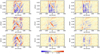 |
Fig. 1 Tomography of the pulsation filtering from the mean line profile residuals. From top to bottom: transits 1, 3, and 4, respectively. Left panels: contour plot of the mean line profile residuals. Central panels: same as for left panels, but after filtering in the Fourier space. Right panels: same as for central panels, after subtracting the best-fit Doppler shadow model. The horizontal white lines show the beginning and end of the transit. |
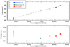 |
Fig. 2 Measurements of the inclination angle i (top panel) and of the projected spin-orbit angle λ (bottom panel) as a function of time. The dashed line shows the linear trend discussed in Sect. 3. |
Stellar and orbital parameters adopted in this work.
4 Radial velocities
Since we could not exploit the cross-correlation functions (CCFs) from the DRS, RVs were extracted following the method presented in Borsa et al. (2019). Instead of using a Gaussian fit, we preferred to model the LSD lines with a rotational profile (Gray 2008). We measured a v sin is = 86.4 ± 0.5 km s−1, taken as theaverage of the out-of-transit measurements and their standard deviation, which is well in agreement with previous values (v sin is = 86.63 km s−1, Johnson et al. 2015). The extracted RVs are listed in Table B.1. We subtracted the difference from the mean of the in-transit RVs from each transit observation to avoid any possible offset caused by instabilities, long-term pulsations, and trends in the orbital solution (e.g. Borsa et al. 2019). We then averaged the RVs of the four transits in bins of 0.005 in phase. The RV time series of each single transit analysed and their average are shown in Fig. 3.
Although stellar pulsations also dominate the RV curve, it is evident a qualitative agreement with the theoretical RM curve calculated using the parameters presented in Table 2 (by using the formalism of Ohta et al. 2005). This is further confirmation that for fast rotators the method of fitting the mean line profiles with a rotational profile instead of a Gaussian function brings optimal results, as was previously found for other targets (e.g. Anderson et al. 2018; Johnson et al. 2018; Borsa et al. 2019; Rainer et al. 2021). We note, however, that for this case the Doppler tomography method remains the preferred one to determine the projected spin-orbit inclination angle.
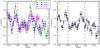 |
Fig. 3 Left panel: phase folded RVs of the three analysed HARPS-N transits of WASP-33b. Different colours refer to different transits. Right panel: RVs of the three transits averaged in bins of 0.005 in phase (filled circles), together with single RVs (small dots). The blue line represents the theoretical RV solution calculated with the parameters of Table 2 (the values of λ and i are obtained from the average of the three transits). |
5 Balmer lines absorption in the transmission spectrum
We studied the atmosphere of WASP-33b using the technique of transmission spectroscopy, focusing on Hα and Hβ absorption, and taking into account the possible contamination given by stellar effects.
5.1 Transmission spectrum extraction
We performed transmission spectroscopy following the method of Wyttenbach et al. (2015), applying the following steps independently to each transit. First, we shifted the spectra to the stellar radial velocity rest frame using a Keplerian model of the system. Then we normalised each spectrum by dividing for the average flux within defined wavelength ranges where telluric and stellar lines are not present.
Using the out-of-transit spectra only, we built a telluric reference spectrum T(λ), by means of a linear correlation between the logarithm of the normalised flux and the air mass (Snellen et al. 2008; Vidal-Madjar et al. 2010; Astudillo-Defru & Rojo 2013), and we then re-scaled all the spectra as if they had been observed at the air mass corresponding to that at the centre of the transit. We then created a master stellar spectrum Smaster by averaging all the out-of-transit spectra (excluding the phase range of the immediate pre-transit, see Sect. 6), and divided all the single spectra for this Smaster creating the residual spectra Sres. Every Sres was then shifted considering the theoretical planetary RV and the systemic velocity of the system, meaning that we placed the spectra in the planetary reference frame. Here, we expect to detect the exoplanetary atmospheric signal centred at the laboratory wavelengths. All the full-in-transit Sres were then averaged to create the transmission spectrum. At this stage, the transmission spectrum of the planet still includes spurious stellar contaminations.
5.2 Removal of CLV + RM
The star over which the planet transits is not a simple homogeneous disc, but it rotates and has a surface brightness that changes as a function of the distance from centre. Effects such as centre-to-limb variations (CLV) and RM have been proven to significantly modify the shape of line profiles, possibly causing false atmospheric detections (e.g. Yan et al. 2017; Borsa & Zannoni 2018; Casasayas-Barris et al. 2020). We thus took these effects into account by creating a model following the methodology described in Yan et al. (2017). The star is modelled as a disc divided into sections of 0.01 Rs. For each point, we calculated the μ value (where μ = cosθ, with θ the angle between the normal to the stellar surface and the line of sight) and the projected rotational velocity (by assuming rigid body rotation and re-scaling the v sin is value of Table 2). A spectrum is then assigned to each point of the grid by quadratically interpolating on μ and Doppler-shifting for the stellar rotation the model spectra created using the tool Spectroscopy Made Easy (SME, Piskunov & Valenti 2017), with the line list from the VALD database (Ryabchikova et al. 2015) and the MARCS (Gustafsson et al. 2008) stellar atmospheric models (assuming local thermodynamic equilibrium approximation). The model spectra are created with null rotational velocity for 21 different μ values, and adapted to the resolving power of the instrument. Then, using the orbital information from Table 2 we simulate the transit of the planet, calculating the stellar spectrum for different orbital phases as the average spectrum of the non-occulted modelled sections. In the last step, we divide each spectrum for a master stellar spectrum calculated out of transit, obtaining the information of the impact of RM + CLV effects at each in-transit orbital phase. We then move everything in the planetary rest frame and calculate the simulated CLV+RM effects on the transmission spectrum (Fig. 4). We note that we do not take into account the possible deformation of the line profiles given by gravity darkening, which are, however, not expected to be significant (see e.g. Kovács et al. 2013).
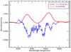 |
Fig. 4 Corrections for CLV + RM and for stellar pulsations applied to the transmission spectrum in the Hα zone. |
5.3 Removal of pulsations
Another contamination one has to deal with in this particular case of WASP-33b comes from the stellar pulsations. In Sect. 3, we show how strongly they impact the mean line profiles. In the same way, they have an impact on the extracted planetary transmission spectrum. To deal with this, we opted for an approach similar to that presented in Borsa & Zannoni (2018) to remove the RM from the transmission spectrum using real observing data. This was done by exploiting the S/N of the mean line profiles. We note that pulsations and RM cannot be removed together in this way. This is because the amplitude of the RM effect is dependent on the planetary effective radius in the narrow band passes where the planetary lines are present. On the contrary, the amplitudes of pulsations vary on a much larger wavelength range and can be assumed constant in each of our narrow band passes of interest. In the following, we make the assumption that the pulsation pattern behaves in the same way for all the absorption lines. We use the pulsation pattern extracted from the mean line profile (which is basically based on metal lines) and assume that it is also valid for the Balmer lines, except for a scaling factor. To justify this assumption, we note that the short periods of δ Sct are not able to produce significant phase shifts between the photospheric stellar lines of different species and excitation potentials. Moreover, the broadening of the Balmer lines largely affects the wings, but not so much the centre, where we search for the in-transit planetary RVs: Balmer and metallic line profiles are very similar there. We also note that we cannot analyse the pulsation pattern directly on the Balmer lines, due to their low S/N. As a final test, we verified that the applied correction does not impact the depth of the retrieved planetary line profile (Sect. 5.4).
We started from the mean line profiles’ residuals after the division for an average out-of-transit mean line profile. We then subtracted the Doppler shadow models calculated in Sect. 3 for each transit (e.g. Fig. 5). Then we created a transmission spectrum of the pulsations (TSpuls) in the wavelength region of interest. First, we put together the three transits, then we move from the velocity to the wavelength space, taking the laboratory wavelength of the Hα (Fig. 6) and Hβ lines as a zero reference, since these are the lines we aim to correct. Then, we moved each mean line-profile residual to the planetary rest frame and averaged the full in-transit residuals to calculate the TSpuls. At this point, we still have to correct for the magnitude of the effect: the calculated TSpuls is in fact referred to a line of which the depth is identical to that of the mean line profile and has to be re-scaled to the depth of the line that we want to correct (Borsa & Zannoni 2018). We thus multiplied the amplitude of the correction for a factor which is the ratio between the depth of the mean line profile and that of the Hα (or Hβ) line, and we obtained the final spectrum used to correct for pulsations (Fig. 4).
5.4 Balmer lines absorption
We corrected the transmission spectrum extracted in Sect. 5.1 from stellar effects by dividing it for the corrective spectra calculated in Sects. 5.2 and 5.3. We note that the effect of pulsations overcome that of CLV + RM by a factor of ~1.5 in magnitude (Fig. 4). We find an excess absorption in the Hα region with a contrast of 0.54 ± 0.04% and a FWHM of 36.7 ± 3.3 km s−1 (Fig. 7). We can translate the contrast into an effective planetary radius Reff = 1.18 ± 0.02 Rp, calculated assuming  , with δ the transit depth (from Table 2) and h the line contrast (e.g., Chen et al. 2020). As for KELT-9b, the Hα profile of WASP-33b forms in the atmospheric region below the Roche lobe, which can be found at about 1.6 planetary radii. Therefore, this detection does not directly probe atmospheric escape, but it would enable one to set constraints on the planetary temperature-pressure structure and thus on the energetics possibly driving escape. The line has a significant blueshift of − 8.2 ± 1.4 km s−1, indicative of winds in the planetary atmosphere. We note that without the correction for the stellar pulsations, we find a comparable depth (0.53%) but a larger FWHM (55 km s−1). As they are non-radial pulsations, their averaged effect on the three transits tends to be smaller in the centre of the stellar line profile, and this is also reflected in the transmission spectrum. This is also noticeable in Figs. 4 and 6.
Checking the reference frame of the detections is fundamental when we want to be sure they are caused by the planetary atmosphere and not by spurious stellar effects (e.g. Brogi et al. 2016; Borsa & Zannoni 2018). This is particularly true for this case, where the strong stellar pulsations may not be perfectly corrected for and could mimic atmospheric features. We thus verified that our Hα absorption detection is in the planetary rest frame by resolving it in the 2D tomographic map (Fig. 8), which shows the position of the absorption signal as a function of the orbital phase.
We also find an excess absorption in the Hβ line region with a contrast of 0.28 ± 0.06%, FWHM of 23.5 ± 6.3 km s−1 and a blueshift of − 6.6 ± 2.6 km s−1 (Figs. 9 and 10). We can translate the contrast into an effective planetary radius Reff = 1.09 ± 0.03 Rp.
We note that the values of absorption depth we obtain are almost half of those obtained for the same planet by Yan et al. (2021) (0.99 ± 0.05% for Hα and 0.54 ± 0.07% for Hβ, respectively). However, the Hα/Hβ line depth ratio is the same (1.93 ± 0.44 for us versus1.83 ± 0.26 for them). Given the fact that another analysis of these lines also shows different line profile depths (1.68 ± 0.02% for Hα and 1.02 ± 0.05% for Hβ, Cauley et al. 2021), we highlight the possibility that the amplitude of the lines could be variable with time and with the level of the stellar activity (e.g. Borsa et al. 2021) and pulsations. We checked within the dataset we analysedand did not find evidence of significant variability among the three transits with the same Hα contrast.
A future common analysis of all available datasets will help to shed light on the possibility of the observed transit depth variations being related to stellar activity and pulsation, rather than being caused by systematics between different analyses. Furthermore, such an analysis will enable one to obtain a very high-quality average line profile for each detected Balmer line. These profiles can then be used tox constrain the temperature structure of the planetary atmosphere in the 10−3–10−9 bar range (e.g. Fossati et al. 2020), going beyond the analysis of Yan et al. (2021), who employed an isothermal profile and assumed local thermodynamical equilibrium. Indeed, it has been shown that, when modelling the Balmer lines detected in the transmission spectrum of the UHJ KELT-9b, these assumptions are invalid (Fossati et al. 2020). Because of similarities in the temperature profile of the upper atmosphere of KELT-9b and WASP-33b (e.g. both present a thermal inversion in the upper atmosphere and reach upper atmospheric temperatures of the order of 10 000 K; Fossati et al. 2018a, 2020), it is likely that the assumptions employed by Yan et al. (2021) to model the Balmer lines led them to obtain unreliable results.
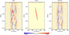 |
Fig. 5 Example of the removal of the Doppler shadow from the mean line profile residuals for transit 4. Left panel: original mean line-profile residuals. Central panel: model of the Doppler shadow. Right panel: mean line profile residuals after the removal of the Doppler shadow. The horizontal white lines show the beginning and end of the transit. |
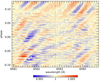 |
Fig. 6 Effect of the pulsation contamination on the three analysed transits as it affects the Hα line, in the stellar rest frame. The vertical dotted line marks the position of the Hα line. The horizontal white lines show the beginning and end of the transit. |
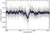 |
Fig. 7 Hα absorption after the correction for stellar effects (RM + CLV and pulsations). Black circles represent 0.1 Å binning. The blue line is the Gaussian best fit. The vertical dotted line shows the planetary Hα rest frame. |
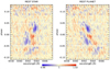 |
Fig. 8 Contour 2D tomography map of Hα absorption in the stellar (left panel) and planetary (right panel) rest frames, before applying the stellar contamination correction (this also evidences the Doppler shadow, i.e. the red track). The white horizontal lines represent the beginning and end of the transit. The vertical dotted black line shows the Hα planetary rest frame in the right panel and the stellar rest frame in the left panel. A pre-transit signal, not centred in the planetary rest frame, is evident (see discussion in Sect. 6). |
6 Pre-transit signal
Looking at the tomographic map of the Hα absorption (Fig. 8), we note a pre-transit feature. This feature has a different slope and duration in the 2D tomographic map with respect to the dominant pulsation pattern in the mean line profiles (see Figs. 1 and 11). We checked the single transits individually and found that this feature looks quite similar in all four available transits (Fig. 11; see the blue diagonal track before the beginning of the transit). It is thus something that happens in an almost coherent timing with the orbital period of the planet.
It appears to be a pseudo-absorption pre-transit signal (PTS) happening on the stellar surface, because it moves from −v sin is to +v sin is (i.e. across the stellar CCF) with time. We thus investigated this more in detail, performing the normalisation on an extended out-of-transit baseline to avoid including the PTS. By visual inspection, we note that a similar behaviour is observed in many single lines, not only on Hα. On the mean line profiles, it is hidden by the other stellar pulsations, but is still noticeable after removing them (Fig. 1, right panel). Curiously, this feature is also reflected in the radial velocities (see Fig. 3).
By studying it on the Hα line and assuming it is moving with a Keplerian motion around the star with the same orbital period of the planet, we found that the rest frame of the PTS is not compatible with the one of the planet. Thus, we define KPTS as the Keplerian semi-amplitude of this pseudo-orbital motion. By fitting Gaussian functions and maximising the contrast of their average, we could estimate that the PTS is moving at a KPTS ~ 460 km s−1 and is centred at phase ~−0.07. As averaged on these values, the PTS has a contrast of 0.61 ± 0.06% (Fig. 12). Curiously, the value of the KPTS is almost double of that of Kp (231 km s−1, Table 2). The two shoulders around the profile (Fig. 12) and the red tracks around the signal (Fig. 11) mimic the presence of a Doppler shadow, but this could possibly be due to a normalisation artifact (e.g. Snellen et al. 2010). Yan et al. (2021) do not find any signs of pre-transit absorption in their Hα analysis of WASP-33b, but we note that they looked in the planetary rest frame only, while we noticed this PTS while looking in the stellar rest frame.
Many photometric transit observations of WASP-33b have been gathered (see Sect. 1), and even if they are affected by the stellar pulsations, none of them reported a pre-transit reduction of flux coherent with the planetary orbital period. The most probable option in our opinion is that the PTS is still a stellar pulsation mode, which is possibly excited by the planetary companion just before the transit. The PTS likely belongs to the same pulsation pattern that is well visible on Hα and Hβ lines in Cauley et al. (2021, see their Fig. 5) and also noticeable in the right panel of Fig. 1. When averaging different transits, the PTS does not average out like the other pulsations, but it tends to clearly stand out beyond the noise. This would indeed be evidence of a somewhat expected star-planet interaction for this system. Mechanisms that can excite stellar pulsations could have tidal or magnetic origin.
Planet-induced stellar pulsations were reported for example in the HAT-P-2 system, where de Wit et al. (2017) discovered pulsation modes corresponding to exact harmonics of the planet’s orbital frequency, which is indicative of a tidal origin. Planetary-induced tides in the host star, manifesting as the second harmonics of the orbital frequency, were also proposed for the systems WASP-12 and WASP-18 (Maciejewski et al. 2020a,b). Tidally induced flux modulations are also shown in heartbeat stars (e.g. Welsh et al. 2011; Thompson et al. 2012) as a result of large hydrostatic adjustments due to the strong gravitational distortion they experience during the periastron passage of the eccentric binary companion. We thus can hypothesise a tidal star-planet interaction to be the cause of the PTS. When considering equilibrium tides, we should find two RV maxima/minima during the planetary orbit, but the effect should be of the order of ~10 m s−1 (i.e. lower than the one seen for WASP-18 considering the masses and orbital configuration of the two systems), thus not detectable. When dealing with pulsations excited by tides instead, their amplitude could be much larger, but the lack of a stellar pulsation frequency close to the expected period of tides (~1.6 days, assuming a stellar rotational period of 0.884 days and a planetary orbital period of 1.22 days) in the frequencies shown in von Essen et al. (2020) is not in favour of this hypothesis. Moreover, the duration of a resonance between pulsations and tides should be very short with respect to the evolutive timescales of the system. The large oscillations produced by the resonance would in fact dissipate a lot of energy, producing an exchange of angular momentum between rotational and orbital motion that modifies both, quickly moving the system out of the resonance. So, the probability that we are observing the system exactly in this moment is low, which also goes against the tidal hypothesis.
Another possibility for the detected PTS is that of a magnetic interaction. Magnetic star-planet interaction has been proposed and observed for some short-period systems, mainly as the modulation of stellar activity index with the orbital period (e.g. Lanza 2009, 2012; Strugarek 2018; Cauley et al. 2019). A pre-transit absorption in the Balmer lines was observed for HD 189733b (Cauley et al. 2015) and was proposed as being caused by the planetary magnetic field, with a bow shock forming around the magnetosphere moving ahead of the planet (Llama et al. 2013; Cauley et al. 2015). Magnetic fields are known to have an effect on stellar pulsations, depending on their magnitude (e.g. Handler 2013, and references therein). The interesting possibility of the PTS being a magnetic excitation of pulsations given by the interaction with the planetary magnetic field could be further explored with spectro-polarimetric measurements, since magnetic fields affect not only the spectral line profiles but also polarisation properties of stellar radiation (e.g. Landi Degl’Innocenti & Landolfi 2004; Oklopčić et al. 2020).
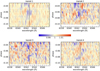 |
Fig. 11 Zoom on the pre-transit signal of the four transits in our dataset, in the stellar rest frame. Vertical line shows the Hα line centre, while vertical dotted lines mark the ± v sin is limits. Horizontal white line shows the beginning of the transit. The pre-transit signal is the diagonal blue track before the beginning of the transit. |
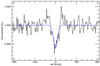 |
Fig. 12 Pre-transit signal profile in its rest frame with KPTS = 460 km s−1. The blue line shows the best-fit Gaussian profile. |
7 Cross-correlation with templates
Since we found the KPTS to be almost double the planetary KP (Sect. 6), we tried to test a possible relation of the PTS with the planetary atmosphere, which could have left aliases, reflections or scattering in the spectra after removing the stellar master. We thus consulted our planetary transmission spectrum for species that could be present only in the planet atmosphere and not in the star. These are to be further investigated in the PTS rest frame in case of detection. We decided to look for Vanadium (V I), which has already been detected in an exoplanetary atmosphere and not in the host star (Ben-Yami et al. 2020; Borsa et al. 2021), and for aluminum oxide (AlO), which has been claimed to be present in the atmosphere of WASP-33b as a result of low-resolution spectrophotometric observations(von Essen et al. 2019).
Planetary atmosphere transmission models were created using petitRADTRANS (pRT, Mollière et al. 2019). We assumed solar abundances, a continuum pressure level of 1 mbar, and an atmospheric temperature-pressure profile calculated for the planet in the same way as presented in Fossati et al. (2020). These parameters were set because they are typical for UHJs (e.g. Hoeijmakers et al. 2019; Stangret et al. 2020). The atmosphericmodels, created in planetary radius as a function of wavelength, were translated into flux (Rp /Rs)2, convolved at the HARPS-N resolving power, and continuum normalised. While for V I we used the opacities already included within pRT, for AlO we used those available at the opacity database of the Exoplanet Simulation Platform1 (Grimm & Heng 2015), which we arranged in the pRT format.
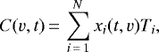
Cross-correlation between the data and the models was performed in the stellar rest frame on single residual spectra after the removal of a master out-of-transit star and telluric contamination (with the procedures explained in Sect. 5) on the whole wavelength range. This was done by working on the bi-dimensional e2ds HARPS-N spectra order by order. We define the cross-correlation as
 (1)
(1)
where T is the model template normalised to unity, and x are the normalised fluxes at the N wavelengths i of the spectra taken at time t and shifted at velocity v. In this way, we preserve the flux information (e.g. Hoeijmakers et al. 2019). In our models, we impose all the values with contrasts of less than 5% of the maximum in the wavelength range to be zero.
We selected a step of 1 km s−1 and a velocity range [−300, 300] km s−1, performing the cross-correlation for each order. We performed a 5σ clipping and masked the wavelength ranges most affected by telluric contamination. Then, for each exposure we applied a weighted average between the cross-correlations of the single orders, where the weights applied to each order are the inverse of the standard deviation (i.e. the larger the S/N, the higher the weight) times the depths of the lines in the model template. For a range of Kp values from 0 to 300 km s−1 (with steps of 1 km s−1), we averagedthe in-transit cross-correlation functions after shifting them in the planetary rest frame. This last step is done by subtracting the planetary radial velocity calculated for each spectrum as vp = Kp × sin2πϕ, with ϕ the orbital phase. In this way, we created the Kp versus Vsys maps, whichare used to test the planetary origin of any possible signal. We evaluated the noise by calculating the standard deviation of the Kp versus Vsys maps far from where any stellar or planetary signal is expected, and in particular where |V | > 90 km s−1.
We find no evidence supporting the presence in the planetary atmosphere either of V I or AlO, giving (model dependent) upper limits of 97 ppm and 17 ppm at the 3σ level, respectively. While for V I we are confident in the accuracy of the line list we used, as it has also already brought a clear detection (Borsa et al. 2021), this is not the case for AlO. We performed an injection of our AlO model in our data using the abundance found in the detection by von Essen et al. (2019), and we were able to recover it with ~14σ significance. Although we did not find evidence of its presence with the available opacities, once an accurate AlO line list is available, verifying the claimed presence of AlO in the planetary atmosphere (von Essen et al. 2019) with high-resolution spectroscopy will be possible using this dataset.
8 Summary and conclusions
We provide further evidence that WASP-33 is undergoing nodal precession, finding a precession period of 1108 ± 19 yr, slightly longer than that determined by Johnson et al. (2015). We also found that the stellar spin is perpendicular to the line of sight, and determined the gravitational quadrupole moment of the star J2 = (6.73 ± 0.22) × 10−5, which is in close agreement with the theoretically predicted value of (6.53 ± 0.41) × 10−5 (e.g. Ragozzine & Wolf 2009). By increasing the time coverage of WASP-33b spectroscopic transit observations it will be possible to further constrain the precession period and possibly, with the growing precision of new-generation instruments, to also detect relativistic effects (Iorio 2016). It would be important to look for other exoplanets in which we can detect orbital precession (other than WASP-33b and Kepler-13Ab), to increase the statistics and understand if this phenomenon may also depend on the presence of other companions, on the value of the stellar rotation, or on the orbital obliquity of the system.
We find that stellar pulsations contaminate the extracted transmission spectrum of the planet and propose a method to de-trend it, which can also potentially be applied to mitigate stellar activity. The detected Hα absorption in the planetary atmosphere extends up to ~1.18 Rp, while absorption in Ca II H&K was detected with an effective radius of ~1.56 Rp (Yan et al. 2019). This confirms the tendency of Ca II H&K and Hα to exist up to the highest layers of the atmospheres of hot Jupiters. The line contrast of the planetary absorption we measured for both Hα and Hβ lines is lower than previously found in the literature (Yan et al. 2021; Cauley et al. 2021), while their contrast ratio is the same. This opens the possibility that the atmosphere of WASP-33b could be sensitive to a variable level of activity of the star.
We detect a pre-transit signal almost coherent with the orbital period of the planet. The most likely explanation is that this is a stellar pulsation mode, which is excited by the planetary companion. The nature of this possible star-planet interaction is still doubtful, even if we tend to exclude tidal interactions and are more in favour of possible magnetic interactions. Spectro-polarimetric observations of the transit and a complete spectroscopic phase coverage, as well as a detailed analysis of stellar pulsations on the line profiles, could help our understanding of the nature of this pre-transit signal.
Acknowledgements
We thank the referee for their useful comments that helped improving the clarity of the manuscript. We acknowledgethe support by INAF/Frontiera through the “Progetti Premiali” funding scheme of the Italian Ministry of Education, University, and Research and from PRIN INAF 2019. FB acknowledges financial support from INAF through the ASI-INAF contract 2015-019-R0.
Appendix A Angular momentum geometry and precession in the WASP-33 system
A.1 Tidal timescales
The tidal timescales of the decay of the obliquity of the WASP-33 system and the exchange of angular momentum between the stellar spin and the orbit can be estimated using the tidal model of Leconte et al. (2010) that we modified to make use of the stellar and planetary modified tidal quality factors,  and
and  , respectively. We adopted
  , a typical value for a Jupiter-like planet, and
  , which corresponds to a strong tidal coupling as expected in late-type stars, but certainly underestimates the tidal timescales for an A-type star (Ogilvie 2014). Possible resonances between tides and stellar pulsations, which could increase the tidal dissipation inside the star, have been excluded by Kovács et al. (2013).
We find a timescale for the decay of the orbital eccentricity of only 0.2 Myr owing to the strong tidal dissipation enforced by the massive star inside the planet, while the decay of the obliquity and the spin-orbit exchange occur on timescales of ~ 300 Myr and ~ 1 Gyr, respectively,because they depend on the much smaller tidal dissipation inside the star. In conclusion, the precession in WASP-33 can be modelled by assuming that the obliquity and the stellar and orbital angular momenta are of constant magnitude, while the orbit can beassumed to have already been circularised (cf. Damiani & Lanza 2011).
A.2 Determining the geometry of the system
The obliquity ϵ of the system is the angle between the angular momentum of the orbital motion, and the spin of the star and is given by (e.g., Damiani & Lanza 2011; Johnson et al. 2015)
 (A.1)
(A.1)
where i is the inclination of the orbital plane, that is, the angle between the line of sight  (i.e. the direction from the observer on Earth to the barycentre of the system) and the orbital angular momentum lorb, is the inclination of the stellar spin axis to the line of sight, and λ is the spin-orbit angle projected onto the plane of the sky, which is measured by fitting the Rossiter-McLaughlin effect or modelling the motion of the Doppler shadow of the planet during its transits. The obliquity ϵ can be assumed constant on the timescales characteristic of the precession (cf. Sect. A.1).
The total angular momentum of the system Ltot is given by the sum of the stellar spin and the orbital angular momentum and is conserved in the absence of external forces (see Fig. A.1). It can be written as follows:
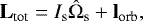 (A.2)
(A.2)
where  is the moment of inertia of the star of mass Ms, equatorial radius Rs, and gyration radius γ, while Ωs is the stellar spin angular velocity that is related to the spectral line rotational broadening as v sin is = ΩsRs sinis.
The modulus of the total angular momentum can be found by taking the scalar product of Eq. (A.2) by itself and considering that  :
:
 (A.3)
(A.3)
where the modulus of the orbital angular momentum for a circular orbit is
 (A.4)
(A.4)
where m = MsMp∕(Ms + Mp) is the reduced mass of the system, Mp the mass of the planet, a the semi-major axis of the orbit, and n = 2π∕Porb the orbital mean motion with Porb being the orbital period.
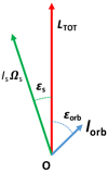 |
Fig. A.1 Total angular momentum of the system Ltot (in red) as resulting from the composition of the stellar spin angular momentum Is Ωs (in green) and the orbital angular momentum lorb (in blue). The angles ϵs and ϵorb between the stellar spin or the orbital angular momentum and the total angular momentum, respectively, are indicated. The obliquity of the system is ϵ = ϵs + ϵorb, while its projection on the plane of the sky is λ (not indicated). |
Since Ltot is constant, taking the scalar product of Eq. (A.2) by the unit vector directed along the line of sight  and making the derivative with respect to the time gives
 (A.5)
(A.5)
where  and
and 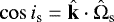 .
.
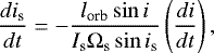
Taking the time derivative of Eq. (A.1), making use of Eq. (A.5), and considering the system at the particular epoch when dλ∕dt = 0 and di∕dt≠0 (as happened in 2011), we obtain an equation that can be solved for is, which is the inclination of the stellar spin to the line of sight:
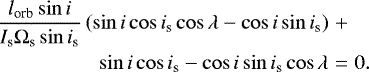 (A.6)
(A.6)
The solution of Eq. (A.6) requires a few iterations because Ωs is derived from the spectroscopic vsinis assuming that the stellar radius Rs is known. The numerical solution converges very rapidly and we adopt the solution closer to π∕2 in our model. In principle, the method can be extended to any epoch when dλ∕dt and di∕dt can both be measured, but the advantage of considering an epoch when dλ∕dt = 0 is that of reducing the errors because the equations simplify and only di∕dt≠0 is required.
To derive the other angles that specify the geometry of the system, we adopted a Cartesian orthogonal reference frame (Oxyz) with the origin O at the barycentre of the system, the polar axis  directed along the total angular momentum, and the
  axis in the plane defined by the vectors Ltot and the line of sight (cf. Fig. A.2).
We introduce the angle β between the total angular momentum Ltot and the unit vector  directed opposite the line of sight, meaning from the barycentre of the system towards the observer, namely
  and
and 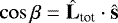 . We also introduced the angles ϵs and ϵorb between the total angular momentum and the stellar spin and orbital angular momentum, respectively; that is,
 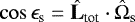 and
and  (see Fig. A.1).
Considering Eq. (A.2) and Fig. A.1, we find the following:
 (A.8)
(A.8)
 (A.9)
(A.9)
 (A.10)
Eqs. (A.8), (A.9), and (A.10) can be used to find the angles β, ϵs, and ϵorb, given that ϵ and is have been derived from Eqs. (A.1) and (A.6), Ltot comes from Eq. (A.3), and the inclination i of the orbital plane is known from the model of the planetary transits.
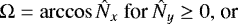
To complete the description of the system, we need to derive the nodal angles αs and αorb between the xz plane, defined by the vectors Ltot and  , and the spin andthe orbital angular momentum, respectively. Since the stellar spin and the orbital angular momentum lie in the same plane containing Ltot, αs = π − αorb, so it is sufficient to derive the latter angle. The components of the unit vector directed along lorb can be expressed as (cf. Fig. A.2)
 (A.11)
Considering the definition of the cross product, we obtain
 (A.12)
By expanding the l.h.s. of Eq. (A.12) by means of Eqs. (A.7) and (A.11), we obtain an equation for αorb:
 (A.13)

Between the two solutions of Eq. (A.13), we chose the one giving the correct sign of
 (A.17)
The values of the angles specifying the geometry of the WASP-33 system are listed in Table A.1 together with their standard deviations. These are obtained by propagating the standard deviations of the system parameters and the systematic deviations obtained by shifting the epoch when dλ∕dt = 0 by 500 days after and before the assumed epoch, respectively.
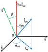 |
Fig. A.2 Reference frame adopted to specify the geometry of the WASP-33 system. The origin O is at the barycentre of the system; the |


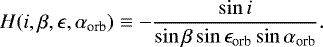
The angles and the factor H(i, β, ϵ, αorb) defining thegeometry and the rate of nodal precession of the WASP-33 system at the epoch 19 October 2011 when dλ∕dt = 0 is assumed. In addition to the standard deviations giving the statistical errors of the parameters, their systematic deviations obtained by shifting the epoch of dλ∕dt = 0 by 500 days after and before 19 October 2011 are listed, respectively.
A.3 Precession of the orbital plane and the stellar spin
The precession of the orbital plane is described by the precession of the vector lorb around the total angular momentum Ltot. In our reference frame, this precession corresponds to a uniform increase (or decrease) of the nodal angle αorb as a function of the time. We can compute the precession rate by differentiating Eq. (A.17) with respect to the time, yielding
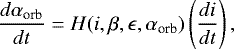 (A.18)
The factor H(i, β, ϵ, αorb) is very close to − 1 in our system (cf. Table A.1), therefore the rate of nodal precession is virtually identical in absolute value to di∕dt. The minimum and maximum values of the inclination of the orbital plane i, reached along a complete precession cycle, can be obtained from Eq. (A.17) for αorb = 0, π and are π − (β ± ϵorb).
Eq. (A.18) can be applied with the observed value of di∕dt to provide the observed rate of precession of the nodes of the planetary orbit; the precession period follows as 2π∕(dαorb∕dt). Alternatively, it can be used with the theoretically derived di∕dt to predict the expected nodal precession rate in our system. Specifically, the theoretical expression of di∕dt for a circular orbit according to Eqs. (7) and (11) of Damiani & Lanza (2011) is
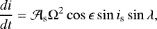 (A.20)
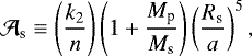
and where k2 is the apsidal motion constant of the star that depends on its internal density stratification (e.g. Claret 2019). We note that the sign of λ as defined by Damiani & Lanza (2011) is opposite that adopted by Johnson et al. (2015) and by the present analysis; Eq. (A.20) has been reformulated according to the latter convention.
The precession of the stellar spin occurs at the same rate as that of the orbital plane, but in the opposite direction, as can be deduced from the conservation of the total angular momentum. The minimum and maximum inclinations of the stellar spin to the line of sight along a precession cycle can be derived as in the case of the orbital plane and are π − (β ± ϵs).
A.4 Gravitational quadrupole moment of the star
The precession rate can be related to the stellar gravitational quadrupole moment J2 by means of Eq. (3) of Johnson et al. (2015), which we recast in our notation as
 (A.22)
We note that our definition of the longitude of the ascending node of the orbit is different from that adopted by Johnson et al., but the precession rate is the same, independently of the definition, because the precession period is unique for the system.
The gravitational quadrupole moment as derived from the observation of the precession of the orbital plane can be compared with the expectation from the theory. Specifically, J2 can be described as the sum of the two components, J2 rot and J2 tide, which are produced by the centrifugal and the tidal distortion of the star, respectively. Their expressions are as follows (e.g. Ragozzine & Wolf 2009):

where G is the gravitation constant. In the case of WASP-33, J2 tide ~ 10−3J2 rot, therefore it can be neglected in our analysis. More precisely, Eq. (A.25) is valid when the planet is on the equatorial plane of the star, but, given the small size of J2 tide, this conclusion is not affected.
Angles Ω and I of the precession model of Iorio (2016) at the epochs of our transit observations.
Finally, we note that we considered the planetary spin synchronised and perpendicular to the orbital plane because tides can enforce such a configuration on a timescale as short as ~ 1 Myr (Leconte et al. 2010). However, if this were not the case, we would have to include the contribution of the planetary gravitational quadrupole moment to the precession of the orbit as discussed by, for example, Ragozzine & Wolf (2009) and Damiani & Lanza (2011). The General Relativity precession is negligible in our case, as it is ~ 500 times smaller than the nodal precession induced by the oblateness of the star (Iorio 2011).
A.5 A comparison with the model of Iorio (2016)
Another model of the precession in WASP-33 was presented by Iorio (2016). It assumes a Cartesian reference frame with the y axis directed towards the observer, the z axis along the projection of the stellar spin on the plane of the sky, and the x axis perpendicular to both the other axes to form a right-handed orthogonal coordinate system (see Fig. 1 of Iorio 2016). In such a reference frame, the precession is described through the variation of the angles Ω, the longitude of the ascending node of the orbit measured from the x axis in the x-y plane, and I, which is the angle between the z axis and the orbital angular momentum. We note that the x-y plane does not coincide with the plane of the sky, while the x-z plane does coincide with it.
The two angles, Ω and I, can be expressed in terms of the inclination i of the orbital plane to the plane of the sky and of the projected obliquity λ on the plane of the sky following Eqs. (25) to (33) of Iorio (2016) as follows:
 (A.26)
 (A.27)
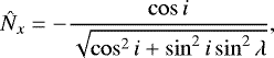
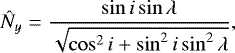

Using the values of i and λ listed by Watanabe et al. (2020) and those derived in the present work, we calculated angles Ω and I and listed them in Table A.2 together with their standard deviations obtained by propagating the errors on the inclination and the projected obliquity. The only two observations available to Iorio (2016) were those of 2008 and 2014 with the parameters i and λ as reported by Johnson et al. (2015), while we adopted the more precise determination of Watanabe et al. (2020). Therefore, Iorio estimated the rate of precession assuming a constant rate of change for both Ω and I between the two epochs that led to an inclination of the stellar spin axis to the line of sight and a stellar quadrupole moment of, in our notation, is = 142° ± 11° and J2 = (2.1 ± 0.8) × 10−4, respectively. Nevertheless, as can be seen in Fig. A.3, the situation was different: the angle I reached a maximum around 2011 and the precession rate dI∕dt became zero at that epoch. By differentiating Eq. (A.30), we see that dI∕dt is zero close to the epoch when dλ∕dt = 0, provided that i is close to 90°, as it is in the case of a transiting planet, although the two epochs only coincide if i = 90°.
Considering Eq. (9) of Iorio (2016) and that his unit vector S* = (0, cosis, sinis) in our notation, for a circular orbit we have (cf. Section A.1):
 (A.31)
where the symbols have been introduced above. For the given values of the angles Ω and I, Eq. (A.31) implies that dI∕dt = 0 when cosis = 0, which confirms our result that the stellar spin is perpendicular to the line of sight around 2011.
The precession rate of the angle Ω at the epochwhen dI∕dt = 0 is given by Eq. (10) of Iorio (2016), that is,
 (A.32)
for a circular orbit. Considering our value of J2 = (6.73 ± 0.22) × 10−5, we obtain a precession rate dΩ∕dt = 0.325 ± 0.015 deg/yr in 2011 that is comparable with the observed mean precession rate 0.353 ± 0.007 deg/yr obtained by a linear regression over the six epochs in Table A.2. We do not expect a closer agreement because the precession rate dΩ∕dt is not constant and the angle I is also variable and affected by relatively large errors. Therefore, we prefer to estimate J2 using Eq. (3) of Johnson et al. (2015), because in that formula the precession rate and the true obliquity ψ are constant, thus allowing a more precise determination.
In conclusion, the differences between the results of Iorio (2016) and ours, as well as those of Watanabe et al. (2020), are due to the paucity of observations available at that time leading to the assumption of constant precession rates for the angles Ω and I. Our more extended dataset allows us to show that the precession rate dI∕dt vanished around 2011, thus reconciling our results with those of Iorio’s study and confirming that the inclination of the stellar spin axis to the line of sight was very close to 90° at that epoch.
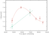 |
Fig. A.3 Angle I of the model by Iorio (2016) versus the time. The red diamonds are the values found from our dataset, while the green triangles are the two values derived by Iorio from the data available to him at the time of his work. We see that the precession rate dI∕dt is not constant as shown by the cubic interpolation plotted as a dotted red line. For the sake of comparison, we plot a linear interpolation between the two values available to Iorio assuming a constant precession rate. |
Appendix B Radial velocity table
HARPS-N RV observations of WASP-33.
References
- Akinsanmi, B., Barros, S. C. C., Santos, N. C., et al. 2019, A&A, 621, A117 [NASA ADS] [CrossRef] [EDP Sciences] [Google Scholar]
- Anderson, D. R., Temple, L. Y., Nielsen, L. D., et al. 2018, MNRAS, submitted [arXiv:1809.04897] [Google Scholar]
- Arcangeli, J., Désert, J.-M., Line, M. R., et al. 2018, ApJ, 855, L30 [NASA ADS] [CrossRef] [Google Scholar]
- Astudillo-Defru, N., & Rojo, P. 2013, A&A, 557, A56 [NASA ADS] [CrossRef] [EDP Sciences] [Google Scholar]
- Ben-Yami, M., Madhusudhan, N., Cabot, S. H. C., et al. 2020, ApJ, 897, L5 [CrossRef] [Google Scholar]
- Borsa, F., & Zannoni, A. 2018, A&A, 617, A134 [NASA ADS] [CrossRef] [EDP Sciences] [Google Scholar]
- Borsa, F., Rainer, M., Bonomo, A. S., et al. 2019, A&A, 631, A34 [NASA ADS] [CrossRef] [EDP Sciences] [Google Scholar]
- Borsa, F., Allart, R., Casasayas-Barris, N., et al. 2021, A&A, 645, A24 [EDP Sciences] [Google Scholar]
- Brogi, M., de Kok, R. J., Albrecht, S., et al. 2016, ApJ, 817, 106 [Google Scholar]
- Casasayas-Barris, N., Palle, E., Yan, F., et al. 2020, A&A, 635, A206 [NASA ADS] [CrossRef] [EDP Sciences] [Google Scholar]
- Cauley, P. W., Redfield, S., Jensen, A. G., et al. 2015, ApJ, 810, 13 [NASA ADS] [CrossRef] [Google Scholar]
- Cauley, P. W., Shkolnik, E. L., Llama, J., et al. 2019, Nat. Astron., 3, 1128 [CrossRef] [Google Scholar]
- Cauley, P. W., Wang, J., Shkolnik, E. L., et al. 2021, AJ, 161, 152 [Google Scholar]
- Chen, G., Casasayas-Barris, N., Pallé, E., et al. 2020, A&A, 635, A171 [CrossRef] [Google Scholar]
- Claret, A. 2019, A&A, 628, A29 [CrossRef] [EDP Sciences] [Google Scholar]
- Claudi, R., Benatti, S., Carleo, I., et al. 2017, Eur. Phys. J. Plus, 132, 364 [CrossRef] [Google Scholar]
- Collier Cameron, A., Bruce, V. A., Miller, G. R. M., et al. 2010a, MNRAS, 403, 151 [NASA ADS] [CrossRef] [Google Scholar]
- Collier Cameron, A., Guenther, E., Smalley, B., et al. 2010b, MNRAS, 407, 507 [NASA ADS] [CrossRef] [Google Scholar]
- Cosentino, R., Lovis, C., Pepe, F., et al. 2012, Proc. SPIE, 8446, 84461V [CrossRef] [Google Scholar]
- Cosentino, R., Lovis, C., Pepe, F., et al. 2014, Proc. SPIE, 9147, 91478C [Google Scholar]
- Covino, E., Esposito, M., Barbieri, M., et al. 2013, A&A, 554, A28 [NASA ADS] [CrossRef] [EDP Sciences] [Google Scholar]
- Damiani, C., & Lanza, A. F. 2011, A&A, 535, A116 [NASA ADS] [CrossRef] [EDP Sciences] [Google Scholar]
- de Wit, J., Lewis, N. K., Knutson, H. A., et al. 2017, ApJ, 836, L17 [NASA ADS] [CrossRef] [Google Scholar]
- Donati, J.-F., Semel, M., Carter, B. D., Rees, D. E., & Collier Cameron, A. 1997, MNRAS, 291, 658 [NASA ADS] [CrossRef] [MathSciNet] [Google Scholar]
- Eastman, J. 2017, Astrophysics Source Code Library, [record ascl:1710.003] [Google Scholar]
- Eastman, J., Gaudi, B. S., & Agol, E. 2013, PASP, 125, 923 [Google Scholar]
- Eastman, J. D., Rodriguez, J. E., Agol, E., et al. 2019, PASP, submitted [arXiv:1907.09480] [Google Scholar]
- Fabrycky, D. C., & Winn, J. N. 2009, ApJ, 696, 1230 [NASA ADS] [CrossRef] [Google Scholar]
- Fossati, L., Koskinen, T., Lothringer, J. D., et al. 2018, ApJ, 868, L30 [NASA ADS] [CrossRef] [Google Scholar]
- Fossati, L., Koskinen, T., France, K., et al. 2018, AJ, 155, 113 [NASA ADS] [CrossRef] [Google Scholar]
- Fossati, L., Shulyak, D., Sreejith, A. G., et al. 2020, A&A, 643, A131 [NASA ADS] [CrossRef] [EDP Sciences] [Google Scholar]
- Gallet, F., Bolmont, E., Bouvier, J., et al. 2018, A&A, 619, A80 [NASA ADS] [CrossRef] [EDP Sciences] [Google Scholar]
- Gray, D. F., 2008, The Observation and Analysis of Stellar Photospheres (Cambridge, UK: Cambridge University Press) [Google Scholar]
- Grimm, S. L., & Heng, K. 2015, ApJ, 808, 182 [NASA ADS] [CrossRef] [Google Scholar]
- Gustafsson, B., Edvardsson, B., Eriksson, K., et al. 2008, A&A, 486, 951 [NASA ADS] [CrossRef] [EDP Sciences] [Google Scholar]
- Handler, G. 2013, Planets, Stars and Stellar Systems. Volume 4: Stellar Structure and Evolution, 207 [NASA ADS] [CrossRef] [Google Scholar]
- Haynes, K., Mandell, A. M., Madhusudhan, N., et al. 2015, ApJ, 806, 146 [NASA ADS] [CrossRef] [Google Scholar]
- Herman, M. K., de Mooij, E. J. W., Huang, C. X., et al. 2018, AJ, 155, 13 [Google Scholar]
- Herman, M. K., de Mooij, E. J. W., Jayawardhana, R., et al. 2020, AJ, 160, 93 [CrossRef] [Google Scholar]
- Herrero, E., Morales, J. C., Ribas, I., et al. 2011, A&A, 526, L10 [NASA ADS] [CrossRef] [EDP Sciences] [Google Scholar]
- Hoeijmakers, H. J., Ehrenreich, D., Kitzmann, D., et al. 2019, A&A, 627, A165 [NASA ADS] [CrossRef] [EDP Sciences] [Google Scholar]
- Iorio, L. 2011, Ap&SS, 331, 485 [NASA ADS] [CrossRef] [Google Scholar]
- Iorio, L. 2016, MNRAS, 455, 207 [NASA ADS] [CrossRef] [Google Scholar]
- Johnson, M. C., Cochran, W. D., Collier Cameron, A., et al. 2015, ApJ, 810, L23 [NASA ADS] [CrossRef] [Google Scholar]
- Johnson, M. C., Rodriguez, J. E., Zhou, G., et al. 2018, AJ, 155, 100 [CrossRef] [Google Scholar]
- Kovács, G., Kovács, T., Hartman, J. D., et al. 2013, A&A, 553, A44 [NASA ADS] [CrossRef] [EDP Sciences] [Google Scholar]
- Landi Degl’Innocenti, E., & Landolfi, M. 2004, Astrophysics and Space Science Library, 307, Polarization in Spectral Lines [Google Scholar]
- Lanza, A. F. 2009, A&A, 505, 339 [NASA ADS] [CrossRef] [EDP Sciences] [Google Scholar]
- Lanza, A. F. 2012, A&A, 544, A23 [NASA ADS] [CrossRef] [EDP Sciences] [Google Scholar]
- Leconte, J., Chabrier, G., Baraffe, I., et al. 2010, A&A, 516, A64 [NASA ADS] [CrossRef] [EDP Sciences] [Google Scholar]
- Lehmann, H., Guenther, E., Sebastian, D., et al. 2015, A&A, 578, L4 [NASA ADS] [CrossRef] [EDP Sciences] [Google Scholar]
- Llama, J., Vidotto, A. A., Jardine, M., et al. 2013, MNRAS, 436, 2179 [NASA ADS] [CrossRef] [Google Scholar]
- Lothringer, J. D., Barman, T., & Koskinen, T. 2018, ApJ, 866, 27 [NASA ADS] [CrossRef] [Google Scholar]
- Maciejewski, G., Niedzielski, A., Villaver, E., et al. 2020a, ApJ, 889, 54 [Google Scholar]
- Maciejewski, G., Knutson, H. A., Howard, A. W., et al. 2020b, Acta Astron., 70, 1 [NASA ADS] [Google Scholar]
- McLaughlin, D. B. 1924, ApJ, 60, 22 [Google Scholar]
- Mkrtichian, D. 2015, IAU General Assembly 29, 2255391 [Google Scholar]
- Mollière, P., Wardenier, J. P., van Boekel, R., et al. 2019, A&A, 627, A67 [NASA ADS] [CrossRef] [EDP Sciences] [Google Scholar]
- Nugroho, S. K., Kawahara, H., Masuda, K., et al. 2017, AJ, 154, 221 [Google Scholar]
- Nugroho, S. K., Gibson, N. P., de Mooij, E. J. W., et al. 2020, ApJ, 898, L31 [Google Scholar]
- Ogilvie, G. I. 2014, ARA&A, 52, 171 [Google Scholar]
- Ohta, Y., Taruya, A., & Suto, Y. 2005, ApJ, 622, 1118 [Google Scholar]
- Oklopčić, A., Silva, M., Montero-Camacho, P., et al. 2020, ApJ, 890, 88 [CrossRef] [Google Scholar]
- Parmentier, V., Line, M. R., Bean, J. L., et al. 2018, A&A, 617, A110 [NASA ADS] [CrossRef] [EDP Sciences] [Google Scholar]
- Piskunov, N., & Valenti, J. A. 2017, A&A, 597, A16 [NASA ADS] [CrossRef] [EDP Sciences] [Google Scholar]
- Piskunov, N., Kupka, F., Ryabchikova, T. A., Weiss, W. W., & Jeffery, C. S. 1995, A&AS, 112, 525 [Google Scholar]
- Ragozzine, D., & Wolf, A. S. 2009, ApJ, 698, 1778 [Google Scholar]
- Rainer, M., Poretti, E., Mistò, A., et al. 2016, AJ, 152, 207 [NASA ADS] [CrossRef] [EDP Sciences] [Google Scholar]
- Rainer, M., Borsa, F., Pino, L., et al. 2021, A&A, 649, A29 [NASA ADS] [CrossRef] [EDP Sciences] [Google Scholar]
- Rossiter, R. A. 1924, ApJ, 60, 1 [NASA ADS] [CrossRef] [Google Scholar]
- Rozelot, J. P., Damiani, C., & Pireaux, S. 2009, ApJ, 703, 1791 [NASA ADS] [CrossRef] [Google Scholar]
- Ryabchikova, T., Piskunov, N., Kurucz, R. L., et al. 2015, Phys. Scr., 90, 054005 [Google Scholar]
- Smith, A. M. S., Anderson, D. R., Skillen, I., et al. 2011, MNRAS, 416, 2096 [NASA ADS] [CrossRef] [Google Scholar]
- Snellen, I. A. G., Albrecht, S., de Mooij, E. J. W., & Le Poole, R. S. 2008, A&A, 487, 357 [NASA ADS] [CrossRef] [EDP Sciences] [Google Scholar]
- Snellen, I. A. G., de Kok, R. J., de Mooij, E. J. W., et al. 2010, Nature, 465, 1049 [Google Scholar]
- Stangret, M., Casasayas-Barris, N., Pallé, E., et al. 2020, A&A, 638, A26 [CrossRef] [EDP Sciences] [Google Scholar]
- Strugarek, A. 2018, Handbook of Exoplanets, 25 [Google Scholar]
- Szabó, G. M., Pál, A., Derekas, A., et al. 2012, MNRAS, 421, L122 [NASA ADS] [CrossRef] [Google Scholar]
- Ter Braak, C. J. F. 2006, Stat. Comput., 16, 239 [Google Scholar]
- Thompson, S. E., Everett, M., Mullally, F., et al. 2012, ApJ, 753, 86 [Google Scholar]
- Vidal-Madjar, A., Arnold, L., Ehrenreich, D., et al. 2010, A&A, 523, A57 [NASA ADS] [CrossRef] [EDP Sciences] [Google Scholar]
- von Essen, C., Czesla, S., Wolter, U., et al. 2014, A&A, 561, A48 [NASA ADS] [CrossRef] [EDP Sciences] [Google Scholar]
- von Essen, C., Mallonn, M., Albrecht, S., et al. 2015, A&A, 584, A75 [NASA ADS] [CrossRef] [EDP Sciences] [Google Scholar]
- von Essen, C., Mallonn, M., Welbanks, L., et al. 2019, A&A, 622, A71 [NASA ADS] [CrossRef] [EDP Sciences] [Google Scholar]
- von Essen, C., Mallonn, M., Borre, C. C., et al. 2020, A&A, 639, A34 [CrossRef] [EDP Sciences] [Google Scholar]
- Watanabe, N., Narita, N., & Johnson, M. C. 2020, PASJ, 72, 19 [CrossRef] [Google Scholar]
- Welsh, W. F., Orosz, J. A., Aerts, C., et al. 2011, ApJS, 197, 4 [Google Scholar]
- Wyttenbach, A., Ehrenreich, D., Lovis, C., et al. 2015, A&A, 577, A62 [NASA ADS] [CrossRef] [EDP Sciences] [Google Scholar]
- Yan, F., Pallé, E., Fosbury, R. A. E., et al. 2017, A&A, 603, A73 [NASA ADS] [CrossRef] [EDP Sciences] [Google Scholar]
- Yan, F., Casasayas-Barris, N., Molaverdikhani, K., et al. 2019, A&A, 632, A69 [NASA ADS] [CrossRef] [EDP Sciences] [Google Scholar]
- Yan, F., Wyttenbach, A., Casasayas-Barris, N., et al. 2021, A&A, 645, A22 [EDP Sciences] [Google Scholar]
All Tables
The angles and the factor H(i, β, ϵ, αorb) defining thegeometry and the rate of nodal precession of the WASP-33 system at the epoch 19 October 2011 when dλ∕dt = 0 is assumed. In addition to the standard deviations giving the statistical errors of the parameters, their systematic deviations obtained by shifting the epoch of dλ∕dt = 0 by 500 days after and before 19 October 2011 are listed, respectively.
Angles Ω and I of the precession model of Iorio (2016) at the epochs of our transit observations.
All Figures
|
Fig. 1 Tomography of the pulsation filtering from the mean line profile residuals. From top to bottom: transits 1, 3, and 4, respectively. Left panels: contour plot of the mean line profile residuals. Central panels: same as for left panels, but after filtering in the Fourier space. Right panels: same as for central panels, after subtracting the best-fit Doppler shadow model. The horizontal white lines show the beginning and end of the transit. |
| In the text | |
|
Fig. 2 Measurements of the inclination angle i (top panel) and of the projected spin-orbit angle λ (bottom panel) as a function of time. The dashed line shows the linear trend discussed in Sect. 3. |
| In the text | |
|
Fig. 3 Left panel: phase folded RVs of the three analysed HARPS-N transits of WASP-33b. Different colours refer to different transits. Right panel: RVs of the three transits averaged in bins of 0.005 in phase (filled circles), together with single RVs (small dots). The blue line represents the theoretical RV solution calculated with the parameters of Table 2 (the values of λ and i are obtained from the average of the three transits). |
| In the text | |
|
Fig. 4 Corrections for CLV + RM and for stellar pulsations applied to the transmission spectrum in the Hα zone. |
| In the text | |
|
Fig. 5 Example of the removal of the Doppler shadow from the mean line profile residuals for transit 4. Left panel: original mean line-profile residuals. Central panel: model of the Doppler shadow. Right panel: mean line profile residuals after the removal of the Doppler shadow. The horizontal white lines show the beginning and end of the transit. |
| In the text | |
|
Fig. 6 Effect of the pulsation contamination on the three analysed transits as it affects the Hα line, in the stellar rest frame. The vertical dotted line marks the position of the Hα line. The horizontal white lines show the beginning and end of the transit. |
| In the text | |
|
Fig. 7 Hα absorption after the correction for stellar effects (RM + CLV and pulsations). Black circles represent 0.1 Å binning. The blue line is the Gaussian best fit. The vertical dotted line shows the planetary Hα rest frame. |
| In the text | |
|
Fig. 8 Contour 2D tomography map of Hα absorption in the stellar (left panel) and planetary (right panel) rest frames, before applying the stellar contamination correction (this also evidences the Doppler shadow, i.e. the red track). The white horizontal lines represent the beginning and end of the transit. The vertical dotted black line shows the Hα planetary rest frame in the right panel and the stellar rest frame in the left panel. A pre-transit signal, not centred in the planetary rest frame, is evident (see discussion in Sect. 6). |
| In the text | |
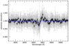 |
Fig. 9 Same as Fig. 7, but for Hβ. |
| In the text | |
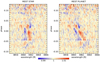 |
Fig. 10 Same as Fig. 8, but for Hβ. |
| In the text | |
|
Fig. 11 Zoom on the pre-transit signal of the four transits in our dataset, in the stellar rest frame. Vertical line shows the Hα line centre, while vertical dotted lines mark the ± v sin is limits. Horizontal white line shows the beginning of the transit. The pre-transit signal is the diagonal blue track before the beginning of the transit. |
| In the text | |
|
Fig. 12 Pre-transit signal profile in its rest frame with KPTS = 460 km s−1. The blue line shows the best-fit Gaussian profile. |
| In the text | |
|
Fig. A.1 Total angular momentum of the system Ltot (in red) as resulting from the composition of the stellar spin angular momentum Is Ωs (in green) and the orbital angular momentum lorb (in blue). The angles ϵs and ϵorb between the stellar spin or the orbital angular momentum and the total angular momentum, respectively, are indicated. The obliquity of the system is ϵ = ϵs + ϵorb, while its projection on the plane of the sky is λ (not indicated). |
| In the text | |
|
Fig. A.2 Reference frame adopted to specify the geometry of the WASP-33 system. The origin O is at the barycentre of the system; the |
| In the text | |
|
Fig. A.3 Angle I of the model by Iorio (2016) versus the time. The red diamonds are the values found from our dataset, while the green triangles are the two values derived by Iorio from the data available to him at the time of his work. We see that the precession rate dI∕dt is not constant as shown by the cubic interpolation plotted as a dotted red line. For the sake of comparison, we plot a linear interpolation between the two values available to Iorio assuming a constant precession rate. |
| In the text | |
Current usage metrics show cumulative count of Article Views (full-text article views including HTML views, PDF and ePub downloads, according to the available data) and Abstracts Views on Vision4Press platform.
Data correspond to usage on the plateform after 2015. The current usage metrics is available 48-96 hours after online publication and is updated daily on week days.
Initial download of the metrics may take a while.