| Issue |
A&A
Volume 652, August 2021
The Early Data Release of eROSITA and Mikhail Pavlinsky ART-XC on the SRG mission
|
|
|---|---|---|
| Article Number | A135 | |
| Number of page(s) | 9 | |
| Section | Stellar atmospheres | |
| DOI | https://doi.org/10.1051/0004-6361/202141379 | |
| Published online | 24 August 2021 | |
Simultaneous eROSITA and TESS observations of the ultra-active star AB Doradus
1
Hamburger Sternwarte,
Gojenbergsweg 112,
21029
Hamburg,
Germany
e-mail: This email address is being protected from spambots. You need JavaScript enabled to view it.
2
Max-Planck-Institut für extraterrestrische Physik,
85748
Garching,
Giessenbachstraße,
Germany
Received:
25
May
2021
Accepted:
14
June
2021
Abstract
We present simultaneous multiwavelength observations of the ultra-active star AB Doradus obtained in the X-ray range with the eROSITA instrument on board the Russian–German Spectrum-Roentgen-Gamma mission, and in the optical range obtained with the Transiting Exoplanet Survey Satellite (TESS). Thanks to its fortuitous location in the vicinity of the southern ecliptic pole, AB Dor was observed by these missions simultaneously for almost 20 days. With the hitherto obtained data we study the long-term evolution of the X-ray flux from AB Dor and the relation between this observable and the photospheric activity of its spots. Over the 1.5 yr of eROSITA survey observations, the “quiescent” X-ray flux of AB Dor has not changed, and furthermore it appears unrelated to the photospheric modulations observed by TESS. During the simultaneous eROSITA and TESS coverage, an extremely large flare event with a total energy release of at least 4 × 1036 erg in the optical was observed, the largest ever seen on AB Dor. We show that the total X-ray output of this flare was far smaller than this, and discuss whether this maybe a general feature of flares on late-type stars.
Key words: X-rays: stars / stars: individual: AB Dor / stars: flare / stars: coronae / stars: activity
Note to the reader: the article was assigned to another Special Issue on 16 December 2021.
© ESO 2021
1 Introduction
Stellar magnetic activity manifests itself as a variety of different phenomena in different parts of the outer stellar atmosphere: star spots are located in the photosphere, plage regions in the chromosphere, and hot, magnetically confined plasma in the corona. The characteristic radiation from these different regions is emitted in the optical range, and at UV and X-ray wavelengths. As the various atmospheric layers are physically interconnected, one needs simultaneous multiwavelength observations – preferably over some extended period of time – to arrive at a better understanding of the interconnection between various activity phenomena.
With the advent of the eROSITA and TESS missions (see a detailed discussion in Sect. 2) a new observational opportunity has opened up that allows us to monitor stars continuously from space at optical and X-ray wavelengths. While the detailed scientific goals and observing strategies for eROSITA and TESS are quite different, they allow simultaneous coverage over several weeks in smaller regions around the poles of the ecliptic. Fortuitously, one of the prototypical ultra-active stars in the solar neighborhood, AB Doradus, at a distance of only d = 15.3 pc from the Sun, is located at large ecliptic latitudes (β = −86.6°), and for this reason AB Dor receives rather extensive simultaneous exposure with the eROSITA (see Sect. 2.1) and TESS satellites (see Sect. 2.2).
The rotation period of AB Dor is very short (P = 0.51 day), and consequently it shows all the typical signatures of magnetic activity such as star spots and chromospheric and coronal emission, the signatures of which we explore in this study. AB Dor A is a member of a quadruple system discussed in detail by Guirado et al. (2011), but the other system components are much fainter and are ignored in the following. AB Dor was first detected as a strong X-ray source with the Einstein Observatory by Pakull (1981), and since then has been observed with most subsequent X-ray satellites: with ROSAT (Kürster et al. 1997), XMM-Newton (Güdel et al. 2001, Lalitha et al. 2013a), and Chandra (Hussain et al. 2007). In addition to showing strong “persistent” X-ray emission, AB Dor frequently flares at X-ray wavelengths, and a detailed statistical study of these X-ray flares is presented by Lalitha (2016), extending an earlier study based on GINGA data by Vilhu et al. (1993). Most relevant for our study is that of Kürster et al. (1997), who analyzed 5 yr of ROSAT X-ray observations of AB Dor, finding no evidence for long-term changes in its X-ray flux and only some partial modulation with its rotation. Lalitha & Schmitt (2013b) analyze the long-term X-ray behavior of AB Dor from multi-satellite data and find that its persistent level of X-ray emission does not show long-term changes by more than a factor of two, possibly modulated along with its photometric variability.
Extensive ground-based photometry of AB Dor taken over decades is available and has been presented by Järvinen et al. (2005); one of the main results of this study is the conclusion that the surface spots of AB Dor are grouped around two active longitudes separated on average by 180° and that they migrate with a variable rate because of surface differential rotation. These studies show the persistent presence of large spots on the surface of AB Dor, which change in size and location over the years; for example, Ioannidis & Schmitt (2020) used TESS data to study the spot surface distribution on AB Dor in 2018 and also find (see their Fig. 4) two major spots that are slowly changing their respective positions with time.
Photometric studies of active stars have been revolutionized by space-based observatories such as CoRoT, Kepler, and TESS both in terms of achievable photometric precision and temporal coverage, because they are not affected by scintillation, day and night, weather, and other effects. Schmitt et al. (2019) present a detailed analysis of optical flares recorded on AB Dor during the first two months of TESS observations, and report the occurrence of eight “superflares”, that is, flares with a total energy release in excess of 1034 erg. Schmitt et al. (2019) show that the occurrence rate of these events is about one per week, and further present a re-analysis of an X-ray flare on AB Dor, which was first described by Lalitha et al. 2013a), demonstrate the superflare nature of this event, and show that the energy release at optical wavelengths likely exceeds that at X-ray wavelengths. Ioannidis & Schmitt (2020), extending these studies by analyzing the full set of TESS AB Dor data obtained during its first year of operations, analyzed – among other things – the spot distribution and its changes and the occurrence of flares with respect to the spot distribution of AB Dor. In particular, the flare occurrence on AB Dor appears to be linked to the presence of the active regions on its visible surface, that is, the chance that a flare will occur is larger when AB Dor is photometrically fainter.
The purpose of this paper is to present the results of the first three eROSITA surveys on AB Dor, with particular emphasis onthe long-term evolution of its X-ray flux and the simultaneous observations obtained between eROSITA and TESS. In Sect. 2 we discuss basic properties of the eROSITA and TESS satellites in as much they are relevant for our study, and in Sect. 3 we present our new observational results on AB Dor.Section 4 contains a discussion and in Sect. 5 we present our conclusions.
2 eROSITA and TESS satellites and data analysis
2.1 The eROSITA instrument on board SRG
The eROSITA instrument (extended ROentgen Survey with an Imaging Telescope Array) is the soft X-ray instrument on board the Russian–German Spectrum-Roentgen-Gamma mission (SRG). After its launch from Baikonur, SRG was placed into a halo orbit around the Sun–Earth L2 point, where it is performing a 4-yr all-sky survey, which started in December 2019. The eROSITA all-sky survey is carried out in a way that is similar to the ROSAT all-sky survey, that is, the sky is scanned in great circles perpendicular to the plane of the ecliptic.
The longitude of the scanned great circle, that is, the survey rate, moves by ~1° per day, and thus the whole sky is covered in half a year; this procedure will be carried out eight times over the life time of the mission, and we refer to the respective data sets as eRASS1 to eRASS8. In this paper we present data from the surveys eRASS1-3.
The eROSITA scan rate is set to 1.5 deg min−1 or one rotation in 4 hours. Thus, given the eROSITA field of view of ~1 deg, a typical single scan exposure can last up to 40 sec. As a consequence of this survey geometry, the periods of elapsed time during which a given source is observed depend sensitively on its ecliptic latitude: sources near the plane of the ecliptic are observed for a day, and sources at high ecliptic latitudes such as AB Dor are observed for a couple of weeks, but always with a cadence of 4 h.
The eROSITA instrument contains seven X-ray telescopes, each equipped with their own CCD camera in the focal plane of the respective telescope. All seven telescopes and cameras are operated independently, but they all look parallel. Except for some slight differences in filters, the seven units are identical, thus providing a high degree of redundancy. The energy range eROSITA is between 0.2 and 8 keV, its spectral resolution approaches 80 eV at an energy of 1 keV, which is significantly higher than that obtained by the ROSAT PSPC and opens up entirely new scientific investigations; a detailed description of the eROSITA hardware, mission, and in-orbit performance is presented by Predehl et al. (2021).
2.2 The TESS satellite
The Transiting Exoplanet Survey Satellite (TESS) was launched on April 18, 2018, into a highly elliptical 13.7 day orbit in a 2:1 resonance with the Moon. This type of orbit provides a very stable environment for its operations, but it also leads to interruptions in the data stream with the same period; a detailed description of the TESS mission is given by Ricker et al. (2015). The primary scientific goal of the TESS mission is the detection of exoplanets around the brighter stars using the transit method, and to this end TESS performs differential photometry for many thousands of stars. TESS is equipped with four red-band optimized wide-field cameras that continuously observe a 24° × 96° strip on thesky for 27 days. Subsequently, the TESS pointing is moved by about 24° along the plane of the ecliptic, and thus a whole hemisphere is covered within a year. In subsequent years observations switched between the northern and southern ecliptic halves of the sky. TESS began its observations on the southern hemisphere prior to the launch of eROSITA. When the eROSITA all-sky survey began in December 2019, TESS was still observing north, but switched then to observations of the southern hemisphere.
2.3 Data analysis: eROSITA
For our eROSITA study of AB Dor, we use the results of the first three of eROSITA’s eight planned all-sky surveys, using the processing results of the eSASS pipeline (currently version 946); a detailed description of this software and the algorithms used is given by Brunner et al. (2021). Briefly, the eSASS system analyzes the incoming photon stream, attaches a sky position and energy to each recorded photon, and sorts the events into sky tiles with a size of 3.6° × 3.6°.
The events organized in sky tiles can be further analyzed, and with the program scrtool photons around a given position can be extracted and light curves constructed including all necessary corrections such as vignetting and dead time. For the studies reported in this paper we used the nominal source of position of AB Dor and an extraction circle with a radius of 72 arcsec to gather all the source photons. The effective area of eROSITA drops significantly for energies in excess of about 2.3 keV, and therefore we only consider events in the energy range 0.2–2.3 keV. To convert from count rate to energy flux, we need an energy conversion factor of (ECF), which depends on the spectral composition of the incident X-ray flux; the derivation of the ECF as used in this paper is presented in Sect. 3.2. We note in this context that all count rates reported in this paper refer to equivalent on-axis count rates for all seven telescopes: due to the scanning nature of eROSITA, even the count rate of a constant source is changing all the time, and the concept of a “mean” observed count rate is not useful, because it would depend on the exposure history of the source, the number of telescopes used, and so on.
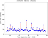 |
Fig. 1 Scan-averaged AB Dor light curve obtained during eRASS1 in December 2019 and January 2020; blue dots: eROSITA data points, dashed red line connects adjacent data points for better visibility. |
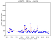 |
Fig. 2 Scan-averaged AB Dor light curve obtained during eRASS2 in June and July 2020: blue dots: eROSITA data points, dashed red line connects adjacent data points for better visibility. |
2.4 Data analysis: TESS
The TESS project provides the light curves of pre-selected targets (which AB Dor belongs to) with a cadence of 2 min; these light curves were generated with the so-called Science Processing Operations Center (SPOC) pipeline, which was derived from the corresponding pipeline for the Kepler mission (Jenkins et al. 2016); further information can be found at the website1. The light curves are publicly accessible and available for download from the Mikulski Archive for Space Telescopes (MAST)2. We specifically use the so-called Simple Aperture Photometry (SAP) fluxes for our analysis.
3 Results
3.1 eROSITA light curves for AB Dor
In Figs. 1–3, we show the eROSITA light curves measured for AB Dor during the eRASS1, eRASS2, and eRASS3 observations; we note that the formal count rate errors are typically smaller than the plot symbols in these figures. Being a strong source with typically (at least) ~40 cts s−1, AB Dor can be detected in almost all scans. To obtain results with reasonable statistics, we only consider scans with at least five counts and more than 3 s of vignetting-corrected exposure, and end up with a total of 319 valid scans obtained during the eRASS1-eRASS3 observations. As discussed above, eROSITA provides “snapshots” of AB Dor’s corona every 4 h during a period of almost three weeks. Given AB Dor’s rotation period of slightly over 12 h, the star rotates by 120° between twosubsequent scans, and after three scans eROSITA views (almost) the same stellar hemisphere again. This implies that subsequent scans represent almost independent samples of the coronal state of AB Dor – at least for coronal regions near the surface.
Variability is a clear characteristic of AB Dor’s X-ray light curve: arbitrarily defining every scan with count rates in excess of 90 cts s−1 as a “flare”, 10 out of the observed 319 scans fall into this category. On the other hand, once flares are excluded, AB Dor appears to have some “memory” as to what its count rate and X-ray flux should be. To quantify the encountered count rate distribution,in Fig. 4 we show a histogram of all valid AB Dor eROSITA scans recorded in the surveys eRASS1-3, together with a log-normal distribution fit to the bulk part of the rate distribution below 100 cts s−1; the best fit parameters are ln(μrate) = 3.72 and σ = 0.23. Around 5% of the distribution are outside the log-normal distribution, and the largest events are discussed in Sect. 3.5.2.
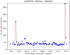 |
Fig. 3 Scan-averaged AB Dor light curve obtained during eRASS3 in December 2020 and January 2021; blue dots: eROSITA data points, dashed red line connects adjacent data points for better visibility. |
3.2 eROSITA spectrum for AB Dor
To illustrate the spectral properties of AB Dor as measured by eROSITA, we present in Fig. 5 a spectrum of the quiescent emission of AB Dor together with a spectral fit composed of two optically thin temperature components with temperatures of (0.66 ± 0.01) keV and (2.03 ± 0.14) keV and variableabundances, which was obtained using the XSPEC package (Arnaud 1996). Figure 5 shows that the X-ray flux of AB Dor as measured by eROSITA is concentrated in the spectral range up to 2.3 keV; the rapid drop in X-ray flux seen between 1 keV and 2 keV is both due to the intrinsic properties of AB Dor’s corona and the rapidly falling effective area of eROSITA. One also notices a strong line near 0.67 keV, which is caused by OVIII Lyα, as well as a much weaker “line” near 0.525 keV, the so-called OVII triplet; one further notices the Ne IX triplet near 1.08 keV and the Fe L complex between 0.8 and 0.9 keV. The plasma model fits the observed spectrum quite well; the formal value of χ2 is 1.19. The ratio between the model flux (in the spectral range 0.2–2.3 keV) and the vignetting-corrected count rate is 1 × 10⁻¹² erg cm−2 ct−1, which is the required ECF to convert from count rate to energy flux. It is difficult to estimate the accuracy of this ECF. A major source of uncertainty is the vignetting correction which depends both on energy and the off-axis angle at which a photon is registered, yet these uncertainties ought to be below 10%. This ECF was used to convert from measured count rate to inferred energy flux for all the AB Dor scans obtained by eROSITA.
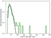 |
Fig. 4 Histogram of AB Dor scan-averaged count rates obtained during eRASS1-3. |
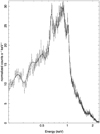 |
Fig. 5 Scan-averaged quiescent X-ray spectrum of AB Dor (black data points) together with a model fit consisting of two isothermal plasma emission models (solid line); see text for more details. |
3.3 TESS light curves for AB Dor
In the following section, we discuss the light curves obtained by TESS concurrent with eROSITA’s coverage of AB Dor during the eRASS3 observations. In Fig. 6 (labels on right y-axis) we plot the TESS SAP flux as a function of time (blue data points). The comparatively much more sparsely sampled eROSITA rates are also plotted for comparison (red data points). The TESS light curve is characterized by its substantial modulation interpreted as rotational modulation through star spots. From late December 2020 to early January 2021, the typical peak-to-peak variation with respect to the mean flux is found to be 22%, quite a bit larger than the 18% peak-to-peak variations found by Schmitt et al. (2019).
A very noticeable feature is the huge flare that occurred on Jan. 7, 2021, peaking at around UT 4:15 and analyzed below. We also phased the TESS light curve of AB Dor folded with a period of 0.514275 days (i.e., the rotation period of AB Dor derived by Schmitt et al. (2019) from TESS data obtained in 2018) and found that this value also provides a good description of the light curve data shown in Fig. 6. Furthermore, our phasing analysis (cf., Fig. 9) also shows that there is very little light curve evolution, which turns out to be extremely useful for the analysis of the large flare.
In Fig. 7, we show some phased TESS light curves obtained around the big flare; we note that the phase interval of unity corresponds to 0.514275 days. In the upper panel of Fig. 7 the light curve during the flare (red data points)is shown as well as the light curve averaged over the rotation prior to and after the flare; fortuitously the light curves before and after the flare are extremely similar, which leads us to assume that the (background) light curve during the flare has also not changed. Modeling this background as the mean of the light curves before and after, we can subtract the nonflare background and obtain the pure flare light curve, also shown in Fig. 7 (black data points in lower panel). As demonstrated by Fig. 7, the whole flare event lasts a little over seven hours. Prior to the actual impulsive event, there appears to be some pre-flare activity lasting almost 3 h. The actual rise to flare peak then occurs in about 30 min. There appears to be some substructure in the flare rise phase, consisting possibly of two events with shorter rise times. After the flare peak, the light curve decreases more or less exponentially and merges into the photospheric background after about 3.5 h, suggesting that the whole flare duration is about 7 h.
This overall flare duration of 7–8 h is considerably longer than AB Dor’s half rotation period of 6.1 h. Doppler imaging (Kürster et al. 1994, Kürster and Schmitt 1996) suggests an inclination angle of AB Dor of around 60°, and therefore on the stellar surface there is a continuity from regions never visible around the “south pole” to regions always visible around the “north” pole. As there are no features in the light curve that suggest rotational modulation of the flare emission, the flare site was likely at some higher latitude, but photometry alone is insufficient to locate the flare site.
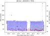 |
Fig. 6 TESS light curve for AB Dor (blue data points, right ordinate) concurrent with eROSITA’s eRASS3 survey observations(red data points, left ordinate). |
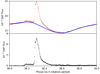 |
Fig. 7 TESS light curve (in terms of 10−4 SAP flux) of the large flare on AB Dor, phased with rotation period. Upper panel: blue data points are the mean of the light curves in rotations before and after the flare, and the red data points are the rotation during the flare. Lower panel: net flare light curve. |
3.4 Analysis of TESS flares
3.4.1 Energetics
To determine the energetics of the flare, we follow the approach outlined by Schmitt et al. (2019). As discussed by Schmitt et al. (2019), the spectral band pass of TESS is relatively broad (it comprises the wavelength range between 6000 Å and 10000 Å centered on the I-band) and captures only some part of the overall flux. For simplicity, we assume blackbody spectra, although the photospheric spectrum of AB Dor is clearly not that of a blackbody, and once the flare sets in, the temperature is continuously varying, yet the TESS data do not allow us to diagnose these changes. To convert the instrumental TESS fluxes into physical values, we assume a bolometric luminosity for AB Dor of 1.5 × 1033 erg s−1, an effective temperature of 5100 K (cf., Close et al. 2007) and a distance of 15.3 pc; in the literature one finds a range of possible effective temperatures, yet those differences lead to rather small changes in the conversion from SAP rates to energy fluxes (in the TESS band).
However, the TESS band captures only part of AB Dor’s overall emission. The fraction of the total flux captured by TESS depends on the temperature and reaches values of ≈0.35 for temperatures near 5000 K. For hotter plasma temperatures, as expected for the flaring plasma, more and more flux is emitted outside the TESS band, and therefore that fraction decreases. By numerically integrating the recorded flare light curve (shown in Fig. 7), we can determine the total SAP count of the flare. To accurately convert SAP count into fluence, we would have to know the evolution of flare temperature with time which is unknown. To stay on the conservative side, we therefore apply the derived photospheric energy conversion factor and estimate a total optical flare energy of 4 × 1036 erg, which is an order of magnitude higher than the most powerful AB Dor flare discussed by Schmitt et al. (2019). We stress that this number is – in the context of our approximations – a lower limit to the actual energy release because the flare temperature always exceeds the photospheric temperature and the energy radiated in the rise phase is missing entirely from our considerations.
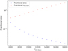 |
Fig. 8 Computed flare filling factor scaled by the surface area of AB Dor (blue data points) and flare bolometric luminosity (at observedflare peak) scaled by its bolometric luminosity (red data points); see text for more details. |
3.4.2 Flare filling factor
Again following the analysis of Schmitt et al. (2019), we can estimate the filling factor of the flare by computing the emitting area from Stefan–Boltzmann’s law, the determined peak luminosity and an assumed flare temperature. At optical flare peak, the plasma temperature was (presumably) much higher, it is therefore interesting to compute these values as a function of the unknown flare effective temperature. In Fig. 8, we present the bolometric instantaneous luminosity of the flare (scaled by the quiescent bolometric luminosity of AB Dor) and compute the flare filling factor (scaled by AB Dor’s surface) as a function of effective temperature. Figure 8 shows that for flare temperatures above about 12 000 K, the bolometric flare luminosity is equal to AB Dor’s bolometric luminosity, while at the same time the flare filling factor is only a few percent. This is a consequence of the T4 dependence of Stefan–Boltzmann’s law. Needless to say, these numbers should be considered as magnitude estimates in view of all the existing uncertainties, yet the calculated flaring area is still small compared to the stellar radius and the overall flare area is still in the one-digit percentage range. In contrast, the spot filling factors required to explain the observed rotational modulations are quite large based on the empirical fitting formulae provided by Maehara et al. (2017) as well as the explicit spot modeling of AB Dor performed by Ioannidis & Schmitt (2020). Using the formulae provided by Maehara et al. (2017), we find a spot filling factor of between 10% and 20% for the whole star, and Ioannidis & Schmitt (2020) require three large spots with typical sizes of 0.15–0.2 R* (cf., Figs. 4 and 5 Ioannidis & Schmitt 2020) in terms of stellar radius to account for the measured brightness variations; we note that for all photospheric modeling, we must assume a temperature difference between a spot and the pristine photosphere.
3.5 Joint analysis of eROSITA and TESS data
We now focus on the data simultaneously taken by the eROSITA and TESS missions, and discuss the properties of AB Dor’s quiescent and flaring emission.
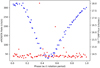 |
Fig. 9 Phased light curve of concurrent eROSITA and TESS data for AB Dor; red data points show the eROSITA count rates (left hand axis), blue data points show the TESS SAP fluxes (right hand axis). |
3.5.1 Quiescent emission
In Fig. 9, we plot the eROSITA (red data points) and TESS light curves (blue data points) obtained during the concurrent eRASS3 observations. We note that the TESS flare data points (shown in Fig. 7) have been left out, while all eROSITA data are shown. To produce the TESS data points, we interpolated between the available measurements around the time for each eROSITA scan, thus producing a TESS light curve with a spacing of 4 h. We also note that for better visibility a constant offset was removed from the TESS data and the subtracted light curve was scaled by a factor of 100. One first notes very little optical light curve evolution during the three weeks of concurrent data taking, that is, during that period the spot configuration on AB Dor stayed more or less constant. Two further X-ray flares can be seen, one near phase 0.62, having occurred on Dec. 22 at 10:32, and another one near phase 0.42, having occurred on Jan. 7 at 6:32; these flares are discussed in Sect. 3.5.2. In contrast to the optical lightcurve, the X-ray light curve shows no apparent structure and a correlation analysis invoking Pearson’s r as well as a Spearman’s rank correlation coefficient formally confirms that optical and X-ray data are uncorrelated, implying that the X-ray emission – at least as observed during eRASS1-3 – does not depend on the rotational phase and therefore does not depend on the spot coverage over the visible hemisphere of AB Dor. As a consequence, it is quite difficult to directly determine rotational modulation from X-ray data for active stars, while such determinations are (usually) straightforward from optical monitoring data.
3.5.2 Flaring emission
In the joint eROSITA/TESS light curve of AB Dor (shown in Fig. 3 and Fig. 6) there are two occasions when eROSITA shows count rates in excess of 100 cts s−1: one on Dec. 22 at 10:32 and another on Jan. 7 at 6:32. The latter event, which is so far the event with the largest count rate observed by eROSITA, is clearly accompanied by an equally huge TESS flare of almost twice the size of the rotational modulation.
For the first of these flares, which is very noticeable in X-rays, there is no conspicuous flare event in the TESS light curve. A very small flare with a duration of less than 8 min is observed about 40 min prior to the time of the eROSITA X-ray scan. Whether or not these events are related to each other cannot be deduced from the available data. However, we can say with confidence that the X-ray flare is not accompanied by any conspicuous energetic optical event.
The situation is very much different for the second flare on Jan. 7. As evident from Fig. 7, the X-ray flare does occur during a major optical flare, and given that the scan 4 h after the peak is still elevated, it is tempting to interpret the X-ray light curve as arising from a long-duration flare event.
The 4-h temporal cadence of eROSITA survey observations is not that well suited for the study of stellar flares. While ideally the X-ray light curve should be continuously covered, for an assessment of the X-ray energetics one needs the peak amplitude Apeak and the flare decay time τdecay, because for an assumed exponential decay the total X-ray energy is proportional to Apeak × τdecay. Furthermore, it is helpful to know the start times of flares and the times of their peaks in order to obtain an assessment of the rise phase, which, however, normally contributes relatively little to the overall energy budget because the rise times tend to be very short. Unfortunately, none of these parameters are accurately known, and therefore a precise determination of the X-ray energetics isimpossible.
Given the extreme nature of the optical flare, the question arises as to what a reasonable X-ray scenario might look like. Given that the optical decay is quite exponential without any substructure, we can assume that the X-ray decay is also purely exponential;as the X-ray rise phase is unobserved, we ignore it in our “modeling”. Needless to say, there are no unique solutions, and to give an idea of what the flare light curve could have looked like, we present a few examples in Fig. 10, where we show the measured eROSITA data (blue points) and the derived TESS flare light curve (scaled by a factor of ten, blue curve). We also show three hypothetical cases, that is, an X-ray flare peak close to the optical flare peak (green curve), an X-ray flare peak close to the observed scan maximum (red curve), and a case in between (magenta). For the simplified chosen models we computed total X-ray outputs of 1.2 × 1035 erg, 6.4 × 1034 erg, and 4.9 × 1034 erg for the green, magenta, and red model curves. Experience shows that the rise phase could contribute an additional 10% or so to the total X-ray output, yet it is difficult to see how any realistic flare scenario would yield an X-ray energy output significantly above 2 × 1035 erg.
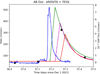 |
Fig. 10 eROSITA X-ray observations (black data points) and TESS flare light curve (blue solid line). Some hypothetical X-ray flare light curves are shown in the colors red, magenta, and green. Red corresponds to a minimal-energy scenario and green is close to a most likely scenario; see text for more details. The left and right axes apply to the X-ray and TESS data, respectively. |
4 Discussion
4.1 Quiescent X-ray and optical emission
A general characteristic of AB Dor’s optical emission are the large modulations observed at almost all times as evidenced by the TESS light curves presented in this paper and those by Schmitt et al. (2019) and Ioannidis & Schmitt (2020). This finding demonstrates the presence of large but inhomogeneously distributed star spots on AB Dor’s surface at all times. The X-ray flux from AB Dor as observed by eROSITA is also variable, however the kind of observed variability is different. Once obvious flare scans are removed, the X-ray snapshots taken by eROSITA can be well characterized by a log-normal distribution which appears to be constant at least over the 1.5 yr of eROSITA observations. In contrast to the optical flux, no significant modulation of the X-ray flux with the rotation period is detected, which one would naively expect by assuming a correlation between larger spot coverage and stronger X-ray emission. The coronae of rapid rotators such as AB Dor should be saturated (for a discussion, see Güdel 2004), and indeed, computing the logarithmic ratio of X-ray and bolometric luminosities for AB Dor, we find log(LX∕Lbol) = −3.17. Therefore, AB Dor’s corona is saturated as expected, and we suspect that this may be responsible for the lack of observed X-ray modulations.
4.2 eROSITA and TESS flares
Both the TESS optical light curves (cf., Schmitt et al. 2019, Ioannidis & Schmitt 2020) and eROSITA X-ray light curves show many flares (cf., Figs. 1–3), which we discuss in this section.
4.2.1 Comparison to optical flares on late-type stars
For the flare on AB Dor on Jan. 7 we determine a (minimal) optical energy of 4 × 1036 erg; to the best of our knowledge this is the most energetic flare event so far observed on AB Dor. Energy releases on that order of magnitude are quite rare, to say the least. Günther et al. (2020) present the results of a specific survey to detect flares on late-typestars using the first months of TESS data, and report the detection of 8695 flares in total, which occurred on 1228 individual stars, out of which 673 are M dwarfs; the relevant data are listed in Tables 1 and 2 in Günther et al. (2020). Out of the 8695 flares reported by Günther et al. (2020), only 11 had total energy releases of above 1036 erg. Closer inspection of the host stars for these large flares reveals a somewhat mixed picture, yet none of these stars appear to be on or near the main sequence; also, 4 of the 11 flares above 1036 erg occurred on the star TIC332487879 (= HD 220096), which again is located far away from the main sequence. If we then restrict attention to late-type stars on or near the main sequence by arbitrarily demanding stellar radii below 1.5 R⊙, we end up with 7074 flares with known energy releases as determined by TESS. The histogram of these flare energy releases is shown in Fig. 11, together with the position of the large flare on AB Dor.
Figure 11 clearly demonstrates the unique character of the event from Jan. 7 from the point of view of energetics; we note that all of the eight superflares on AB Dor described by Schmitt et al. (2019) are located in the bulk of the distribution shown in Fig. 11, emphasizing our point that the flare from Jan. 7 represents a very unique event not only for AB Dor. This statement does not imply that K/M dwarfs cannot produce flares with energy releases above 1036 erg; for example, using ground-based observations with the NGST, Jackman et al. (2019), report the detection of a flare with an energy release of ≈3 × 1036 erg on a pre-main sequence star at a distance of 210 pc, and Davenport (2016) report flares observed by the Kepler telescope in a sample biased towards G-type stars, some of which produce flare energy releases up to 1037 erg, albeit on rather distant stars. This is in line with the findings of Wu et al. (2015), also based on Kepler studies of G-type stars, who report flare energy releases in the range 1036 –1037 erg in their sample.
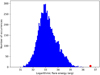 |
Fig. 11 Histogram of total flare energy outputs from TESS measurements of 7074 flares on late-type stars (blue filled histogram, data taken from Günther et al. 2020) and the AB Dor flare from Jan. 7 (red hexagon, this paper); see text for more details. |
4.2.2 Flares simultaneously observed by eROSITA and TESS
Focusing now on the data simultaneously covered by eROSITA and TESS, there are two X-ray flares with scan-averaged count rates in excess of 100 cts s−1 or LX > 2.5 × 1030 erg s−1. While the X-ray flare on Dec. 22 at 10:32 shows very little or no optical emission, the opposite holds for the Jan. 7 flare at 6:32. We visually inspected the TESS light curve and can state with certainty that there are no additional major flares to the Jan. 7 flare described in Sect. 3.5.2.
Clearly, the temporal sampling of the X-ray light curve is somewhat sparse, and so we are unsure of how certain we can be about the derived energetics. In this context, we again note that the total energy release of a flare is essentially determined by only two numbers, the peak amplitude and the decay time. Wu et al. (2015) clearly demonstrate (see their Fig. 5) thatthe flares with the largest energy releases are those with the longest decay times. The same is also true when X-ray flares are considered, some examples are presented by Tsuboi et al. (2000) for energetic flares on the protostars YLW15 and Schmitt & Favata (1999) and Schmitt et al. (2003) present examples for flares on Algol.
Fortunately, in the case of the AB Dor flare on Jan. 7, we have two eROSITA data points in the decay phase, which allows us to put rather stringent constraints on the overall energy output. In the idealistic case of a purely exponentially decaying flare with an instantaneous rise phase, the decay time can be easily computed from the measured amplitudes and times (A1, t1) and (A2, t2) through 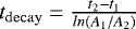 , which in our case yields a decay time value of about 10 500 s, with some error. The amplitude A0 at flare onset is then given by
  , where Δt denotes the (unknown) time difference between flare peak and the first available measurement. We stress that our ignorance of Δt constitutes the major source of error in our estimates. However, we can constrain Δt: experience from other flares leads us to expect that the flare peak should have occurred a short time after the optical flare peak, which suggests Δt ≈ 7000 s. We know for sure that during the scan prior to the optical flare peak no X-ray flare was ongoing (see Fig. 3), that is, we have Δt < 14 000 s. We therefore expect A0 ≈ 2 × A1, and we know for sure A0 < 4 × A1. Clearly, Δt could be smaller than 7000 s, which would then reduce the total energy output in X-rays. A purely exponential decay is admittedly only an approximation, and the rise phase is missing altogether from our considerations. In our case, there may be some substructure in the optical rise phase, while the decay phase appears very smooth. We therefore argue that it is likely that the X-ray decay was also very close to being exponential, and in practically all major TESS flares the rise phases are much shorter than the decay phases. Considering all of this evidence, we find it difficult to avoid the conclusion that the X-ray energy release in the event from Jan. 7 was significantly less than the optical energy release.
4.3 The bigger picture
There is broad agreement in the literature that the primary energy release of solar and stellar flares takes place in the corona and involves magnetic energy and nonthermal energetic particles. The nonthermal particles produced in the corona propagate along the magnetic field lines to reach denser and cooler regions, where they dissipate their energy, thus producing heating. As a consequence, both the optical emission recorded by TESS as well as the soft X-ray emission recorded by eROSITA are secondary if not tertiary flare products, and therefore an assessment of the overall energetics and the contribution of the various sources and wavelength ranges to the overall energy budget is notoriously difficult even for solar flares. For the case of the large solar X17 flare from October 25, 2003, Woods et al. (2004) present such an analysis and conclude that the majority of the energy of the flare is released at wavelengths longward of 200 nm and shortward of 27 nm. Specifically, Woods et al. (2004) find that 19% of the observed total solar irradiance measurements (TSI) change occurs in the XUV and X-ray range, while the UV range between 270 Å and 2000 Å contributes only 3.7%, which means that almost 80% of the energy output is observed in the optical. Thus, the ratio of X-ray to optical output is about 1:4, while for the large flare on AB Dor we estimate 1:20 with, admittedly, considerable uncertainty.
The immediate question that comes to mind is whether this is a general property of AB Dor flares. The flare observed on Dec. 22 presents an obvious counter example, because its peak X-ray luminosity of 4 × 1030 erg s−1 is accompanied by very little or possibly no detectable optical emission. Nevertheless, we need to bear in mind the fact that optical flare light curves are affected by projection and limb-darkening effects. A very nice example in this context is provided by the Sun, as already discussed by Schmitt et al. (2019): the already mentioned solar flare from October 25, 2003 is the largest one so far observed in TSI, for which Kopp et al. (2005) present a detailed analysis and derive a total flare energy release of 5 × 1032 erg. However, probably the largest solar flare measured in modern times, namely the class X40 flare discussed by Brodrick et al. (2005) occurring on November 3, 2003, right at the solar limb in the very same active region, was consequently – in contrast to the X-ray range – only very faintly visible in TSI data (Kopp et al. 2005). Therefore, the observed ratio of the X-ray and optical outputs may differ a lot, while the intrinsic ratio may not. In the solar case, the flare site is usually known and projection and limb-darkening effects can be assessed, while for spatially unresolved stars the flare site on the stellar surface remains typically unknown in purely photometric data. On the other hand, as shown by Wolter et al. (2008), in the case of the active star BO Mic, a star actually quite similar to AB Dor, Doppler imaging does in fact allow the flare site to be located on the star.
5 Conclusions
We present the eROSITA observations of the nearby ultra-active star AB Dor from the first three eROSITA surveys; the third (eRASS3) survey was accompanied by simultaneous TESS observations in the optical. We find a “base” level of AB Dor’s X-ray flux, which appears essentially constant over 1.5 yr, and no evidence for rotational modulation in the X-ray flux, which we attributeto the saturated nature of AB Dor’s corona. During the eRASS3 observation, a major flare occurred on AB Dor, and the large amount of energy released makes it the largest ever observed on this star. Estimating the total X-ray output from the simultaneously measured eROSITA light curve, we find an X-ray output at least a factor of ten smaller. A comparison to large solar flares suggests quite a few similarities and we point out the limitations of optical observations, which usually do not reveal the flare site on the star. We therefore conclude that the measurement of the total energy budget of solar and stellar flares is a challenge, and it remains to be seen whether big flares in general emit intrinsically more energy in the optical than in the X-ray range.
Acknowledgements
This work is based on data from eROSITA, the soft X-ray instrument aboard SRG, a joint Russian–German science mission supported by the Russian Space Agency (Roskosmos), in the interests of the Russian Academy of Sciences represented by its Space Research Institute (IKI), and the Deutsches Zentrum für Luft- und Raumfahrt (DLR). The SRG spacecraft was built by Lavochkin Association (NPOL) and its subcontractors, and is operated by NPOL with support from IKI and the Max Planck Institute for Extraterrestrial Physics (MPE). The development and construction of the eROSITA X-ray instrument was led by MPE, with contributions from the Dr. Karl Remeis Observatory Bamberg & ECAP (FAU Erlangen-Nürnberg), the University of Hamburg Observatory, the Leibniz Institute for Astrophysics Potsdam (AIP), and the Institute for Astronomy and Astrophysics of the University of Tübingen, with the support of DLR and the Max Planck Society. The Argelander Institute for Astronomy of the University of Bonn and the Ludwig Maximilians Universität Munich also participated in the science preparation for eROSITA. The eROSITA data used for this paper were processed using the eSASS/NRTA software system developed by the German eROSITA consortium. This paper includes data collected by the TESS mission, which are publicly available from the Mikulski Archive for Space Telescopes (MAST).
References
- Arnaud, K. A. 1996, Astron. Data Anal. Softw. Syst. V, 101, 17 [NASA ADS] [Google Scholar]
- Brodrick, D., Tingay, S., & Wieringa, M. 2005, J. Geophys. Res. (Space Phys.), 110, A09S36 [NASA ADS] [CrossRef] [Google Scholar]
- Brunner, H., Liu, T., Lamer, G., et al. 2021, A&A, submitted [arXiv:2106.14517] (eROSITA SI) [Google Scholar]
- Close, L. M., Thatte, N., Nielsen, E. L., et al. 2007, ApJ, 665, 736 [NASA ADS] [CrossRef] [Google Scholar]
- Davenport, J. R. A. 2016, ApJ, 829, 23 [Google Scholar]
- Güdel, M. 2004, A&ARv, 12, 71 [CrossRef] [Google Scholar]
- Güdel, M., Audard, M., Briggs, K., et al. 2001, A&A, 365, L336 [Google Scholar]
- Günther, M. N., Zhan, Z., Seager, S., et al. 2020, AJ, 159, 60 [Google Scholar]
- Guirado, J. C., Marcaide, J. M., Martí-Vidal, I., et al. 2011, A&A, 533, A106 [NASA ADS] [CrossRef] [EDP Sciences] [Google Scholar]
- Hussain, G. A. J., Jardine, M., Donati, J.-F., et al. 2007, MNRAS, 377, 1488 [NASA ADS] [CrossRef] [Google Scholar]
- Ioannidis, P., & Schmitt, J. H. M. M. 2020, A&A, 644, A26 [NASA ADS] [CrossRef] [EDP Sciences] [Google Scholar]
- Jackman, J. A. G., Wheatley, P. J., Pugh, C. E., et al. 2019, MNRAS, 482, 5553 [NASA ADS] [CrossRef] [Google Scholar]
- Järvinen, S. P., Berdyugina, S. V., Tuominen, I., Cutispoto, G., & Bos, M. 2005, A&A, 432, 657 [Google Scholar]
- Jenkins, J. M., Twicken, J. D., McCauliff, S., et al. 2016, Proc. SPIE, 9913, 99133E [Google Scholar]
- Kopp, G., Lawrence, G., & Rottman, G. 2005, Sol. Phys., 230, 129 [NASA ADS] [CrossRef] [Google Scholar]
- Kürster, M., & Schmitt, J. H. M. M. 1996, A&A, 311, 211–29 [Google Scholar]
- Kürster, M., Schmitt, J. H. M. M., & Cutispoto, G. 1994, A&A, 289, 899 [NASA ADS] [Google Scholar]
- Kürster, M., Schmitt, J. H. M. M., Cutispoto, G., & Dennerl, K. 1997, A&A, 320, 831 [NASA ADS] [Google Scholar]
- Lalitha, S. 2016, Solar and Stellar Flares and their Effects on Planets, 320, 155 [Google Scholar]
- Lalitha, S., & Schmitt, J. H. M. M. 2013, A&A, 559, A119 [NASA ADS] [CrossRef] [EDP Sciences] [Google Scholar]
- Lalitha, S., Fuhrmeister, B., Wolter, U., et al. 2013, A&A, 560, A69 [NASA ADS] [CrossRef] [EDP Sciences] [Google Scholar]
- Maehara, H., Notsu, Y., Notsu, S., et al. 2017, PASJ, 69, 41 [Google Scholar]
- Neidig, D. F. 1989, Sol. Phys., 121, 261 [NASA ADS] [CrossRef] [Google Scholar]
- Pakull, M. W. 1981, A&A, 104, 33 [NASA ADS] [Google Scholar]
- Predehl, P., Andritschke, R., Arefiev, V., et al. 2021, A&A, 647, A1 [EDP Sciences] [Google Scholar]
- Ricker, G. R., Winn, J. N., Vanderspek, R., et al. 2015, J. Astron. Telescopes Instrum. Syst., 1, 014003 [Google Scholar]
- Schmitt, J. H. M. M., & Favata, F. 1999, Nature, 401, 44 [NASA ADS] [CrossRef] [Google Scholar]
- Schmitt, J. H. M. M., Ness, J.-U., & Franco, G. 2003, A&A, 412, 849 [NASA ADS] [CrossRef] [EDP Sciences] [Google Scholar]
- Schmitt, J. H. M. M., Ioannidis, P., Robrade, J., et al. 2019, A&A, 628 [Google Scholar]
- Tsuboi, Y., Imanishi, K., Koyama, K., et al. 2000, ApJ, 532, 1089 [CrossRef] [Google Scholar]
- Vilhu, O., Tsuru, T., Collier Cameron, A., et al. 1993, A&A, 278, 467 [NASA ADS] [Google Scholar]
- Woods, T. N., Eparvier, F. G., Fontenla, J., et al. 2004, Geophys. Res. Lett., 31, L10802 [Google Scholar]
- Wolter, U., Robrade, J., Schmitt, J. H. M. M., et al. 2008, A&A, 478, L11 [NASA ADS] [CrossRef] [EDP Sciences] [Google Scholar]
- Wu, C.-J., Ip, W.-H., & Huang, L.-C. 2015, ApJ, 798, 92 [Google Scholar]
All Figures
|
Fig. 1 Scan-averaged AB Dor light curve obtained during eRASS1 in December 2019 and January 2020; blue dots: eROSITA data points, dashed red line connects adjacent data points for better visibility. |
| In the text | |
|
Fig. 2 Scan-averaged AB Dor light curve obtained during eRASS2 in June and July 2020: blue dots: eROSITA data points, dashed red line connects adjacent data points for better visibility. |
| In the text | |
|
Fig. 3 Scan-averaged AB Dor light curve obtained during eRASS3 in December 2020 and January 2021; blue dots: eROSITA data points, dashed red line connects adjacent data points for better visibility. |
| In the text | |
|
Fig. 4 Histogram of AB Dor scan-averaged count rates obtained during eRASS1-3. |
| In the text | |
|
Fig. 5 Scan-averaged quiescent X-ray spectrum of AB Dor (black data points) together with a model fit consisting of two isothermal plasma emission models (solid line); see text for more details. |
| In the text | |
|
Fig. 6 TESS light curve for AB Dor (blue data points, right ordinate) concurrent with eROSITA’s eRASS3 survey observations(red data points, left ordinate). |
| In the text | |
|
Fig. 7 TESS light curve (in terms of 10−4 SAP flux) of the large flare on AB Dor, phased with rotation period. Upper panel: blue data points are the mean of the light curves in rotations before and after the flare, and the red data points are the rotation during the flare. Lower panel: net flare light curve. |
| In the text | |
|
Fig. 8 Computed flare filling factor scaled by the surface area of AB Dor (blue data points) and flare bolometric luminosity (at observedflare peak) scaled by its bolometric luminosity (red data points); see text for more details. |
| In the text | |
|
Fig. 9 Phased light curve of concurrent eROSITA and TESS data for AB Dor; red data points show the eROSITA count rates (left hand axis), blue data points show the TESS SAP fluxes (right hand axis). |
| In the text | |
|
Fig. 10 eROSITA X-ray observations (black data points) and TESS flare light curve (blue solid line). Some hypothetical X-ray flare light curves are shown in the colors red, magenta, and green. Red corresponds to a minimal-energy scenario and green is close to a most likely scenario; see text for more details. The left and right axes apply to the X-ray and TESS data, respectively. |
| In the text | |
|
Fig. 11 Histogram of total flare energy outputs from TESS measurements of 7074 flares on late-type stars (blue filled histogram, data taken from Günther et al. 2020) and the AB Dor flare from Jan. 7 (red hexagon, this paper); see text for more details. |
| In the text | |
Current usage metrics show cumulative count of Article Views (full-text article views including HTML views, PDF and ePub downloads, according to the available data) and Abstracts Views on Vision4Press platform.
Data correspond to usage on the plateform after 2015. The current usage metrics is available 48-96 hours after online publication and is updated daily on week days.
Initial download of the metrics may take a while.