| Issue |
A&A
Volume 652, August 2021
|
|
|---|---|---|
| Article Number | A53 | |
| Number of page(s) | 27 | |
| Section | Numerical methods and codes | |
| DOI | https://doi.org/10.1051/0004-6361/202140653 | |
| Published online | 12 August 2021 | |
Well-balanced treatment of gravity in astrophysical fluid dynamics simulations at low Mach numbers
1
X Computational Physics (XCP) Division and Center for Theoretical Astrophysics (CTA), Los Alamos National Laboratory, Los Alamos, NM 87545, USA
e-mail: philipp@slh-code.org
2
Heidelberger Institut für Theoretische Studien, Schloss-Wolfsbrunnenweg 35, 69118 Heidelberg, Germany
3
Faculty of Physics and Astronomy, Würzburg University, Am Hubland, 97074 Würzburg, Germany
4
Department of Mathematics, Würzburg University, Emil-Fischer-Str. 40, 97074 Würzburg, Germany
5
Zentrum für Astronomie der Universität Heidelberg, Astronomisches Rechen-Institut, Mönchhofstr. 12-14, 69120 Heidelberg, Germany
6
Zentrum für Astronomie der Universität Heidelberg, Institut für Theoretische Astrophysik, Philosophenweg 12, 69120 Heidelberg, Germany
Received:
24
February
2021
Accepted:
29
June
2021
Context. Accurate simulations of flows in stellar interiors are crucial to improving our understanding of stellar structure and evolution. Because the typically slow flows are merely tiny perturbations on top of a close balance between gravity and the pressure gradient, such simulations place heavy demands on numerical hydrodynamics schemes.
Aims. We demonstrate how discretization errors on grids of reasonable size can lead to spurious flows orders of magnitude faster than the physical flow. Well-balanced numerical schemes can deal with this problem.
Methods. Three such schemes were applied in the implicit, finite-volume SEVEN-LEAGUE HYDRO code in combination with a low-Mach-number numerical flux function. We compare how the schemes perform in four numerical experiments addressing some of the challenges imposed by typical problems in stellar hydrodynamics.
Results. We find that the α-β and deviation well-balancing methods can accurately maintain hydrostatic solutions provided that gravitational potential energy is included in the total energy balance. They accurately conserve minuscule entropy fluctuations advected in an isentropic stratification, which enables the methods to reproduce the expected scaling of convective flow speed with the heating rate. The deviation method also substantially increases accuracy of maintaining stationary orbital motions in a Keplerian disk on long timescales. The Cargo–LeRoux method fares substantially worse in our tests, although its simplicity may still offer some merits in certain situations.
Conclusions. Overall, we find the well-balanced treatment of gravity in combination with low Mach number flux functions essential to reproducing correct physical solutions to challenging stellar slow-flow problems on affordable collocated grids.
Key words: hydrodynamics / methods: numerical / convection
© ESO 2021
1. Introduction
Astrophysical modeling often involves self-gravitating fluids. They are commonly described by the equations of fluid dynamics with a gravitational source term – viscous effects are negligible in most astrophysical systems and therefore the nonviscous Euler equations are used. Such systems can attain stationary equilibrium configurations in which a pressure gradient balances gravity, that is hydrostatic equilibrium. A prominent example are stars, modeled in classical approaches as spherically symmetric gaseous objects. Apart from this dimensional reduction, the assumption of hydrostatic equilibrium considerably simplifies the modeling of the – in reality rather complex – structure of stars. The resulting equations of stellar structure (e.g., Kippenhahn et al. 2012) enable successful qualitative modeling of the evolution of stars through different stages. The price for this success is a parametrization of multidimensional and dynamical processes that limits the predictive power of such theoretical models and requires their calibration with observations. Recent attempts to simulate inherently multidimensional and dynamical processes, such as convection in stellar interiors (e.g., Browning et al. 2004; Meakin & Arnett 2006, 2007; Woodward et al. 2015; Rogers et al. 2013; Viallet et al. 2013; Pratt et al. 2016; Müller et al. 2016; Cristini et al. 2017; Edelmann et al. 2019; Horst et al. 2020), have tried to overcome this shortcoming.
Such simulations pose a number of challenges to the underlying numerical techniques. Not only is the range of relevant spatial and temporal scales excessive, but the flows of interest arise in a configuration that is often close to hydrostatic equilibrium. This has two implications: (i) The schemes must be able to preserve hydrostatic equilibrium in stable setups over a long period of time compared to the typical timescales of the flows of interest. (ii) The flow speed v expected to arise from a small perturbation of the equilibrium configuration should be slow compared to the speed of sound c, thus the corresponding Mach number, ℳ ≡ v/c, is expected to be low.
If we decide to avoid approximating the equations and include all effects of compressibility, aspect (ii) above calls for special low-Mach-number solvers in numerical fluid dynamics combined with time-implicit discretization to enable time steps determined from the actual fluid velocity instead of the speed of sound as required by the CFL stability criterion (Courant et al. 1928) of time-explicit schemes. The propagation of sound waves is irrelevant for the problems at hand. Several suitable methods are implemented in the SEVEN-LEAGUE HYDRO (SLH) code. Numerical and theoretical details are discussed in Barsukow et al. (2017b,a), Edelmann & Röpke (2016), Miczek et al. (2015), Edelmann (2014), and Miczek (2013), and examples of the application to astrophysical problems can be found in Horst et al. (2020), Röpke et al. (2018), Edelmann et al. (2017), Michel (2019), and Bolaños Rosales (2016).
Aspect (i), however, also requires attention. The condition for hydrostatic equilibrium is part of the equations of stellar structure, that are discretized and numerically solved in classical stellar evolution modeling approaches. In contrast, hydrostatic equilibrium is only a special solution to the full gravo-hydrodynamic system at the level of the partial differential equations, but it is not guaranteed that discretizations of these equations can reproduce the physically correct equilibrium state. This is in particular the case because gravitational source terms are usually treated in an operator-splitting approach, resulting in different discretizations of the pressure and gravity terms. Astrophysical fluid dynamics simulations often employ finite-volume schemes, in which hydrodynamical flows are modeled with a Godunov-type flux across cell interfaces. Hydrodynamical quantities are therefore determined at these locations. The gravitational source term, in contrast, is discretized in a completely different and independent way. In a second-order code, for example, it is often calculated using cell-averaged densities assigned to cell centers. In general, this procedure does not lead to an exact cancellation of gravity and pressure gradient in hydrostatic configurations. Spurious motions are introduced that mask the delicate low-Mach-number flows arising from perturbations of this equilibrium, such as, for instance, convection driven by nuclear energy release.
To overcome the problem of aspect (i), so-called well-balancing methods have been introduced, which are numerical methods that ensure exact preservation of certain stationary states. Methods of this type have predominantly been developed for the simulation of shallow-water-type models in order to resolve stationary solutions such as the lake-at-rest solution without numerical artifacts (e.g., Brufau et al. 2002; Audusse et al. 2004; Bermudez & Vázquez 1994; LeVeque 1998; Desveaux et al. 2016a; Touma & Klingenberg 2015; Castro & Semplice 2018; Barsukow & Berberich 2020). These stationary states can be described using an algebraic relation, which favors the development of well-balanced methods. In the simulation of hydrodynamics under the influence of a gravitational field, the situation is different, since hydrostatic solutions are described by a differential equation that admits a large variety of solutions that depend on temperature and chemical composition profiles, as well as the equation of state (EoS). In practice, the concrete hydrostatic profile is determined by equations describing physical processes other than hydrodynamics and gravity, such as thermal and chemical transport and the change in energy and species abundance due to reactions.
Different approaches can be used to deal with this: The majority of well-balanced methods for the Euler equations with gravity, for example Chandrashekar & Klingenberg (2015), Desveaux et al. (2016b), Touma et al. (2016), and references therein, are designed to only balance certain classes of hydrostatic states, often isothermal, polytropic, or isentropic stratifications, under the assumption of an ideal gas EoS. However, for many astrophysical applications, in particular, cases involving late stellar evolutionary stages and massive stars, nonideal effects of the gas may be important. In stellar interiors, the most important additions to the ideal gas EoS are radiation pressure and electron degeneracy effects. This requires a more complex – often in parts tabulated – EoS to properly describe the thermodynamical properties of the gas. We discuss an example of such an EoS in Sect. 2.2.2. Well-balanced methods which are capable of balancing hydrostatic states for general EoS have been introduced by Cargo & Le Roux (1994), Käppeli & Mishra (2014, 2016), Grosheintz-Laval & Käppeli (2019), Berberich et al. (2018, 2019, 2020, 2021), and Berberich (2021).
Most methods that have been discussed in the astrophysical context and literature (e.g., Zingale et al. 2002; Perego et al. 2016; Käppeli et al. 2011; Käppeli & Mishra 2016; Popov et al. 2019) balance a second-order approximation of the hydrostatic state rather than the hydrostatic state itself. Another recent approach is the well-balanced, all-Mach-number scheme by Padioleau et al. (2019). None of these publications tested a low-Mach-number, well-balanced method in more than one spatial dimension in a stable stratification over long timescales. As we show in this paper, long-term stability cannot be automatically inferred from one-dimensional (1D) tests, yet it is of fundamental importance for applications in stellar astrophysics.
Using a staggered grid, which in this context means storing pressure on the cell interfaces instead of the cell centers, can alleviate some of the problems of well-balancing the atmosphere, as shown, for example, in the MUSIC code (Goffrey et al. 2017, Sect. 6). For this approach, it still has to be shown that convective velocities scale correctly with the strength of the driving force at low Mach numbers, which we found very challenging in our approach, see Sect. 5.3.
The methods introduced in Berberich et al. (2018, 2019, 2021) can balance any hydrostatic stratification exactly. The only assumption is that the hydrostatic solution to be balanced is known a priori. This poses no severe restriction for many astrophysical applications where the initial condition is often constructed under the assumption of hydrostatic equilibrium. An example are simulations of stellar convection, where the initial model is commonly derived from classical stellar evolution calculations that by construction impose hydrostatic equilibrium. In this context exact well-balancing refers to preserving an initial state, which can be calculated to arbitrary precision, and not to the exactness of other input physics, such as the EoS.
Here, we discuss three possible well-balancing methods that follow rather different approaches. The first method extends the work of Cargo & Le Roux (1994) which only applied to 1D setups into the three-dimensional (3D) case and achieves well-balancing by modifying the pressure part of a general EoS. We refer to this as the Cargo–LeRoux (CL) well-balancing method. The other two methods modify how variables are extrapolated to the cell interfaces. We refer to them as the α-β well-balancing (Berberich et al. 2018, 2019) and the deviation well-balancing method (Berberich et al. 2021). For these three schemes, we describe their theoretical background and study their impact on the accuracy of solutions to a set of simplified test problems, which are designed to resemble typical situations in astrophysics.
The structure of the paper is as follows: Sect. 2 reviews the basic set of equations of fluid dynamics and their implications. It also introduces the notation that is used in the subsequent sections. In Sect. 3 we discuss the discretization of these equations and describe the AUSM+-up flux used in the later tests. The well-balancing schemes are introduced in Sects. 4.1–4.3. In Sect. 5 we test the applicability of the well-balancing methods and their performance in an extensive suite of simple application examples. Conclusions are drawn in Sect. 6.
2. Equations of compressible, ideal hydrodynamics
This section introduces the general set of equations that are solved with the SLH code in their formulation in general coordinates. The following subsections closely follow the presentation of Miczek (2013).
2.1. Compressible Euler equations
We employ curvilinear coordinatesx = (x, y, z) = (x1, x2, x3) with a smooth mapping,
to Cartesian coordinates ξ = (ξ, η, ζ) = (ξ1, ξ2, ξ3). The reasoning here is that the coordinates ξ simplify the computations, while the coordinates x are adapted to the physical object, such as a spherical star.
The compressible Euler equations on curvilinear coordinates then read
with the vector u of conserved variables and the fluxes fξl given by
for l = 1, 2, 3. Here, density and pressure are denoted by 𝜚 and p, respectively. The velocity vector, expressed through its curvilinear components, reads v = (u, v, w) and enters the equation for the total energy density  with the specific energy ϵ and the gravitational potential ϕ. The inclusion of the potential in the total energy does not lead to numerical difficulties here because it is similar in magnitude to the internal energy in a stellar context in general and in all the test problems presented in Sect. 5 in particular. This is possibly different in other situations, where one of the energies is much larger and cancellation errors can become a problem.
The Euler Eq. (2) in their curvilinear form in depend on the derivatives of the coordinate transformation. Its Jacobi determinant is
where ϵlmn is the three-dimensional Levi-Civita symbol. The normal vector nξl and interface area Aξl in ξl-direction are
External forces that enter Eq. (2) are – with an exception discussed below – collectively denoted by the source term s. While there are different possible contributions, for example energy generation due to nuclear burning, gravity inevitably appears in any astrophysical setup. At the same time it might pose difficulties for hydrodynamical codes to maintain hydrostatic solutions to Eq. (2) (see Sect. 2.3) if it includes a strong gravitational source term as is common in the interior of stars. When gravity is the only source term, the expression for s reads
This adds gravitational forces to the momentum part of Eq. (2). The presence of a gravitational field also affects the evolution of total energy. We include this effect in the definition of the total energy rather than the source term, since this treatment significantly improved our accuracy in numerical experiments. We found this to be crucial in simulations of low Mach number convection.
The source term adds gravitational force to the momentum equations. For our current treatment and test setups, the gravitational potential ϕ is fixed in time and changes the mass distribution during the simulation is excluded, meaning self-gravity is neglected. It is a reasonable simplification if the setup is very close to hydrostatic equilibrium and the change in the mass distribution is negligible. Such an approximation, however, fails for stellar core simulations at later evolutionary stages, where asymmetries in the mass distribution may arise due to violent convective motions. However, these setups are not the typical use cases of the well-balancing techniques presented in this paper as deviations from hydrostatic equilibrium are nonnegligible. In our notation lower indices do not indicate partial derivatives to avoid confusion.
2.2. Equation of state
The common choice to close the Euler system Eq. (2) is using an EoS. There are few physically relevant EoS which can be given in a short, explicit analytical form. Two of these are discussed in the following. We assume that all components of the gas are in local thermodynamic equilibrium, that is they can all be described with a common temperature.
2.2.1. Ideal gas
The ideal gas is one of the simplest EoS, yet with a wide range of applications. It describes an ensemble of randomly moving, noninteracting particles in thermodynamic equilibrium. It is an acceptable model for terrestrial gases, such as air, for which the interactions between the particles are small. It serves well in the case of a fully ionized plasma, such as in the interior of stars, as long as the effects of degeneracy and radiation pressure are small.
The ideal gas pressure is given by
with the temperature
The gas constant R for the ideal gas is 8.31446261815324 × 10⁷ erg K−1 mol−1. The specific heat ratio γ depends on the internal degrees of freedom in the underlying gas mixture, typical values are 5/3 for monatomic gases and 7/5 for diatomic gases. For our treatment, it is convenient to write the ideal gas EoS in the form of Eq. (7) depending on the temperature T instead of the explicit dependence of ϵ. We use this form of the EoS to formulate hydrostatic equilibria with certain temperature profiles.
2.2.2. Helmholtz equation of state
While the ideal gas is a useful approximation of the EoS of stellar interiors, it does not capture the effect of partially or fully degenerate electrons or of radiation pressure. A commonly used EoS that includes these effects to great precision is the Helmholtz EoS (Timmes & Swesty 2000). It relies on a interpolation of the Helmholtz free energy from tabulated values using biquintic Hermite polynomials. All other quantities are then derived from expressions involving derivatives of the Helmholtz free energy. This approach ensures that all thermodynamic consistency relations are fulfilled automatically. This EoS has a wide range of applicability and serves as a typical example of a general tabulated EoS, contrasting our approaches to some well-balanced methods relying on using a specific EoS, such as the ideal gas.
2.3. Hydrostatic solutions
Except for the very late stages of stellar evolution, stars can be considered as gaseous spheres, which change only over very long timescales, much longer that those of the fluid motions. Dynamical processes acting in the interiors, as for example convective motions, however, evolve on much shorter timescales. Thus, in hydrodynamical simulations that aim to follow such fast processes, a star can, to first order, be described as a static stratification with pressure and density profiles constant in time, that is

These conditions reduce the first and the last part of Eq. (2) to the trivial relations

The momentum equations lead to the hydrostatic equation
This equation is invariant under transformations between different sets of curvilinear coordinates. A pair of constant-in-time functions 𝜚 and p, which satisfy Eq. (11) together with the chosen EoS is called hydrostatic solution or hydrostatic equilibrium. Since the EoS usually depends on temperature, there is in many cases a whole continuum of hydrostatic solutions rather than uniqueness.
2.3.1. Convective stability
Depending on the stratification, perturbations to the hydrostatic solution may lead to dynamical phenomena. One important example is convection, where hydrostatic equilibrium is not perfectly fulfilled anymore but deviations are small.
The criterion for stability against convection is typically derived by considering the behavior of a small fluid element being perturbed from the surrounding stratification. The frequency at which the element oscillates around its equilibrium position χ0 is called the Brunt–Väisälä frequency N. Its square is given by
where χ denotes the vertical coordinate1, 𝜚int is the density of the small fluid element, and 𝜚ext is the density of the background stratification. It is assumed that the fluid element changes its state adiabatically, that is without exchanging heat with its surrounding, and the derivative ∂𝜚int/∂χ is interpreted as the adiabatic change of density while maintaining pressure equilibrium with the background stratification at height χ. For the full derivation of Eq. (12) we refer the reader to any textbook on stellar astrophysics (e.g., Maeder 2009; Kippenhahn et al. 2012).
It is common to express the gradients in Eq. (12) in terms of different variables. In the case of homogeneous composition (μ(x) = const.) Eq. (12) is equivalent to
![$$ \begin{aligned} N^2 = - \frac{\partial \phi }{\partial \chi } \frac{\partial }{\partial \chi }\left(\frac{s}{c_{\rm p}}\right) = - \frac{\partial \phi }{\partial \chi } \frac{\delta }{T} \left[ \frac{\partial T}{\partial \chi } - \left(\frac{\partial T}{\partial \chi }\right)_{\rm ad} \right], \end{aligned} $$](/articles/aa/full_html/2021/08/aa40653-21/aa40653-21-eq14.gif)
with specific entropy s and specific heat at constant pressure cp and the equation of state derivative,

which is 1 in the ideal gas case. The subscript “ad” denotes the adiabatic derivative as mentioned above.
Another common form of this equation is using a variant of the temperature gradients expressed using pressure as a coordinate,

Using this definition Eq. (12) is equivalent to
with the pressure scale height,
We call a hydrostatic equilibrium stable with respect to convection or convectively stable, if N2 ≥ 0. Otherwise we call it unstable with respect to convection or convectively unstable. This is a local definition, which means that a hydrostatic solution can be convectively stable in one region and convectively unstable in another. A suitable reference time for convectively stable setups is the minimal Brunt–Väisälä time
It seems to be a natural timescale for the evolution of small perturbations as explained for example in Berberich et al. (2019). For any hydrostatic solution, the value of N2 can be either calculated analytically (for simple EoS, like the ideal gas EoS) or numerically for more complex EoS.
Another useful timescale is the sound crossing time tSC through the domain. Similar to Käppeli & Mishra (2016), we define tSC in the direction of coordinate ξl as
with  and
and  being the lower and upper boundaries of the domain in that direction. The speed of sound c is calculated using the equation of state. An expression for the sound speed using a general equation of state is given by
where the function for the pressure p comes from an equation of state (see Sect. 2.2).
3. Discretization
Analytic solutions to Eq. (2) as for example given by the hydrostatic solution of Sect. 2.3 are exceptions and require special initial conditions. To obtain more general solutions, which also allow for more complex dynamics such as turbulent convection developed from perturbations in a hydrostatic stratification, Eq. (2) needs to be solved numerically. While there are several different numerical approaches, this section focuses on the methods that are employed by the SLH code. For a more general introduction on this topic, see Toro (2009).
3.1. Finite-volume scheme
For the numerical solution, the underlying equations have to be discretized on a, possibly curvilinear, mesh that resembles the physical spatial domain. This grid is then mapped to Cartesian coordinates on which the computations are conducted. A set of integers (i, j, k) denotes the center of the (i, j, k)-th cell while, for example, (i + 1/2, j, k) denotes the interface between cell (i, j, k) and (i + 1, j, k). The semi-discrete finite-volume scheme is obtained by integrating Eq. (2) over the cell volume in computational space, leading to
where Vijk is the volume of the corresponding cell in physical space and  ,
,  , and
, and  are the interface areas of the interfaces in ξ, η, and ζ-direction respectively. Details on the computation of cell volumes and interface areas are computed to second order following Kifonidis & Müller (2012). The cell-averaged source term is approximated to second order by
where 𝜚ijk is the cell-averaged value of density and the cell-centered gravitational acceleration  is computed analytically from the given gravitational potential ϕ.
In Eq. (21),  is an approximation of the interface flux for l = 1, 2, 3. There is some freedom in constructing the approximate flux function that calculates
  and many approaches can be found in the literature. However, the specific choice is crucial for the accuracy of the numerical solution. This is further discussed in Sect. 3.2 in the context of flows at low Mach numbers

where c is the speed of sound given by Eq. (20).
The values that enter the approximate flux function need to be reconstructed from the center of the cells to the corresponding interfaces. The reconstruction and the evaluation of the flux is done for each coordinate direction separately, before the resulting fluxes over the surfaces are added for each cell.
The semi-discrete scheme is then evolved in time using an ODE solver, such as a Runge–Kutta method. With an at least linear reconstruction and a sufficiently accurate ODE solver this discretization yields a second-order accurate scheme as has been numerically verified by Berberich et al. (2019). For the tests in this article we mainly use the implicit second-order accurate three step Runge–Kutta method ESDIRK23 of Hosea & Shampine (1996).
We chose an advective CFL time step (CFLu), not strictly for reasons of stability, but as a good compromise between accuracy and efficiency. In curvilinear coordinates it takes the form
with a constant cCFL of order unity and an estimate of the cell length in direction ξl given by
and accordingly for (Δξ2)ijk and (Δξ3)ijk.
This time step criterion generally works well when the flow is fully developed, but it has problems when the Mach numbers on the grid are very small (e.g., in the beginning of a simulation with zero initial velocities), because this yields very large or infinite time steps. As a way to prevent this, Miczek (2013) suggests to include the free-fall signal velocity in the time step calculation. The so-called CFLug time step is then given by
with the signal velocity

The parameter al selects the right branch of the quadratic solution and is given in Table 1.
For Mach numbers close to M = 1, however, it is usually more efficient to use explicit time stepping. For this we use the third-order accurate RK3 scheme of Shu & Osher (1988) with a CFLuc time step controlled by the fluid velocity and sound speed. It is given by
where Ndim denotes the spatial dimensionality of the equations. In contrast to the previous criteria, this is a strict stability criterion for the explicit time stepping. We note that the use of a third-order scheme is not strictly necessary for the presented results. A second-order time integration scheme, such as RK2 (Shu & Osher 1988), yields virtually identical results in combination with second-order spatial reconstruction.
3.2. Numerical flux functions
A fundamental part of the discretization is the choice of a numerical two-state flux. These fluxes give approximate solutions of the two-state Riemann problem at the cell interfaces. Choosing different numerical fluxes yields different properties for the scheme. Many of the typically used Riemann solvers or other flux functions suffer from excessive Mach number dependent diffusion. In the case of the Roe solver (Roe 1981) the origin of this is an upwind term in the schemes that is needed for numerical stability (e.g., Turkel 1987; Guillard & Viozat 1999; Miczek et al. 2015). Other Godunov-type schemes are subject to similar issues (Guillard & Murrone 2004). To correct this behavior, a number of low Mach number fixes have been proposed that aim on reducing the excessive diffusion and make it independent of the Mach number (e.g., Turkel 1987; Li & Gu 2008; Rieper 2011; Oßwald et al. 2015; Miczek et al. 2015; Barsukow et al. 2017a; Berberich & Klingenberg 2020).
One peculiarity of astrophysical setups compared to, for example, setups in the engineering community is the presence of strong stratifications where pressure and density may change by orders of magnitudes within the computational domain. In such setups, the reduction of diffusion comes with the risk of reducing stability and many of the schemes found in the literature develop instabilities. The SLH code is designed in a modular fashion that facilitates the implementation and testing of different types of flux functions. In numerical tests we find the so-called AUSM+-up method to yield appropriate results in the low-Mach regime in combination with the well-balancing method discussed here. The basic construction and a modification for improved low-Mach behavior is discussed here.
An approach to numerical flux functions that can easily be extended to flows at low Mach numbers is followed in the class of Advective Upstream Splitting Methods (AUSM), which have been first introduced by Liou & Steffen (1993). In Liou (1996) the AUSM scheme was extended to AUSM+, the idea of which we briefly describe in the following. To be consistent with the original publication, we use dimensionalized quantities.
The central idea is to split the analytical flux function fχ of Eq. (2) into a pressure and a mass flux via
with
![$$ \begin{aligned} \dot{m}_i = {\varrho } { v}_i,\,\quad \psi = \begin{pmatrix} 1 \\ u\\ { v}\\ { w}\\ E+\frac{p}{{\varrho }} \end{pmatrix},\quad i\in [1,2,3] \end{aligned} $$](/articles/aa/full_html/2021/08/aa40653-21/aa40653-21-eq43.gif)
and the i-th canonical basis vector in the five-dimensional flux vector space ei. This formulation is given for Cartesian coordinates, a transformation to curvilinear coordinates is possible.
The pressure and mass flux of Eq. (29) are discretized separately which results in the numerical flux function

where the upwind term ψup is given by
The core properties of this numerical flux function are determined by the definition of the interface values p1/2 and ṁ1/2 of the pressure p and the mass flux ṁi. With the initially proposed definitions of Liou (1996), this flux function is not capable of resolving low Mach number flows. However, Liou (2006) extended the AUSM+ scheme to AUSM+-up with enhanced low Mach number capability.
For AUSM+-up, the interface pressure is defined as

where  are fifth degree polynomial functions, c1/2 is an approximation for the interface speed of sound, and Ku is a constant that can be set to a value between zero and unity. We refer the reader to Liou (2006) for the detailed definitions of the terms. The third term on the right hand side of Eq. (33) that includes velocity-diffusion is called u-term and is designed to reduce the numerical dissipation at low Mach numbers. It involves a scaling factor fa defined as
with
![$$ \begin{aligned} {{M_\mathrm{o} }}=\min \left[1,\max \left({{\text{ Ma}}},{{M_{\rm cut}}}\right)\right], \end{aligned} $$](/articles/aa/full_html/2021/08/aa40653-21/aa40653-21-eq49.gif)
where Mcut is a cut-off Mach number that ensures that fa does not approach 0 in the limit of very small Mach numbers. This is necessary to prevent singularities as the inverse of fa enters into the mass-flux part (see Eq. (36)) in the original definition of AUSM+-up. However, as described below, the SLH code sets the scaling in these two parts independently such that Mcut can be theoretically set to zero. In SLH, for implementation reasons the value is set to a small value, typically to 10−13, to avoid divergence at smaller Mach numbers. This could easily be changed, but does not have a practical influence on our calculations. The mass flux in AUSM+-up is given by
with the interface Mach number

Here,  are fourth degree polynomial functions and
  . Kp and σ are constants between zero and unity. The last term is called the p-term and is a pressure diffusion term that was introduced to ensure pressure–velocity coupling at low speeds (Edwards & Liou 1998). In the original AUSM+-up scheme the Mach number dependent scaling of the p-term,
  , was chosen identical to that of the u-term, fa. Similar to Miczek (2013) we chose independent cut-off values for fa and
![$$ \begin{aligned} {{f_a^{p}}}=M_o^p (2-M_{o}^p),\quad M_o^p=\min \left[1,\max \left(M,{{M_{\rm cut}^p}}\right)\right]. \end{aligned} $$](/articles/aa/full_html/2021/08/aa40653-21/aa40653-21-eq55.gif)
This way,  can be defined with a significantly higher cut-off Mach number (typically around 10−1) compared to fa. This prevents stability issues, which can occur at locally very low Mach numbers when
  becomes exceedingly large. We use this modified scheme in the presented tests and refer to it as AUSM+-up. Still even this scheme is struggling with maintaining a simple hydrostatic stratification as shown in Sect. 5.1.
It is important to note that the role of the effect of the pressure diffusion is altered by combining AUSM+-up with any of the well-balancing methods described in the following: well-balancing techniques lead to an exact reconstruction of the hydrostatic pressure. Only the nonhydrostatic pressure deviations are captured by the reconstruction and given to the numerical flux. Hence, when well-balancing is applied, the pressure diffusion acts on the nonhydrostatic pressure only.
We define a corresponding basic scheme called  by setting
  . This scheme does have high dissipation at low Mach numbers and we just use it to assess the interaction of the various well-balanced schemes with low Mach number flux functions.
4. Well-balancing methods
To illustrate the issue with configurations close to hydrostatic equilibrium in finite-volume codes we consider the effect of one time step on an initial configuration in perfect hydrostatic equilibrium. For simplicity we discretize the time derivative using the forward Euler method and only consider the one-dimensional Euler equations. From the analytic result we expect that this step will not alter the states and any subsequent steps will also keep the hydrostatic equilibrium intact. To this end we associate a discrete stationary solution that provides a good approximation to the hydrostatic equilibrium. If starting from a discrete hydrostatic equilibrium, the solution of the time evolutionary problem does not change for a numerical scheme, we call it well-balanced.
The density, momentum, and total energy after one time step of length Δt (denoted by the superscript “1”) are calculated from the previous values (denoted by the superscript “0”), the interface fluxes  , and the cell-centered source term
  . The result for cell i is
![$$ \begin{aligned} {\varrho }_i^1&= {\varrho }_i^0 - \frac{\Delta t}{\Delta x}\left[ \left(\hat{\boldsymbol{F}}_{i+{\frac{1}{2}}}^0\right)_1 - \left(\hat{\boldsymbol{F}}_{i-{\frac{1}{2}}}^0\right)_1\right],\end{aligned} $$](/articles/aa/full_html/2021/08/aa40653-21/aa40653-21-eq62.gif)
![$$ \begin{aligned} ({\varrho } u)_i^1&= ({\varrho } u)_i^0 - \frac{\Delta t}{\Delta x}\left[ \left(\hat{\boldsymbol{F}}_{i+{\frac{1}{2}}}^0\right)_2 - \left(\hat{\boldsymbol{F}}_{i-{\frac{1}{2}}}^0\right)_2\right] + \Delta t \left(\hat{\boldsymbol{S}}_i\right)_2,\end{aligned} $$](/articles/aa/full_html/2021/08/aa40653-21/aa40653-21-eq63.gif)
![$$ \begin{aligned} E_i^1&= E_i^0 - \frac{\Delta t}{\Delta x}\left[ \left(\hat{\boldsymbol{F}}_{i+{\frac{1}{2}}}^0\right)_3 - \left(\hat{\boldsymbol{F}}_{i-{\frac{1}{2}}}^0\right)_3\right], \end{aligned} $$](/articles/aa/full_html/2021/08/aa40653-21/aa40653-21-eq64.gif)
where the indexes outside the parentheses stand for the vector component of the flux or source term. To be well-balanced, a scheme needs to guarantee that the step leaves the state unchanged, which leads to the conditions
As the fluxes are evaluated at different states, none of these conditions is fulfilled automatically. A consistent numerical flux will automatically satisfy Eqs. (42) and (44) because the 1- and 3-components of the fluxes are zero for u = 0. The case of Eq. (43) is less straightforward. Here, the discretization of the source term must be constructed to match the flux difference in the hydrostatic case. The methods described in the following subsections achieve this in different ways.
4.1. Cargo–LeRoux method
4.1.1. The one-dimensional Cargo–LeRoux method
One method to turn almost any hydrodynamics scheme into a well-balanced scheme was suggested by Cargo & Le Roux (1994) (see also Le Roux 1999). The only prerequisites it needs are support for a general equation of state and flux functions that resolve contact discontinuities. For completeness we describe the original method, which is only applicable in the one-dimensional case, and turn to the multidimensional extension in Sect. 4.1.2. The one-dimensional Euler equations with gravity read
with g being the, possibly negative, gravitational acceleration in the x-direction. The 1D method presented here relies on gravity being constant in space and time. Furthermore,  is the total energy excluding potential energy. It is only used in the one-dimensional method in this subsection. The multidimensional extension in Sect. 4.1.2 follows a slightly different principle using the total energy E including the potential as defined in Sect. 2.
Cargo & Le Roux (1994) suggest the introduction of a potential q defined by its spatial and temporal derivatives
Numerically, this potential is treated like a composition variable, meaning that its time evolution is determined by the advection equation,
This ensures that the conditions of Eq. (46) are fulfilled at all times if they are satisfied initially.
Expressing the right side of Eq. (45) using q yields
Collecting derivatives with respect to the same variable and inserting 0 = q − q results in
At this point we introduce a modified EoS based on an arbitrary original EoS by defining a new pressure, Π, and total energy per volume, F, as

With this definition Eq. (49) takes the form of the homogeneous Euler equations for a modified EoS,
The physical meaning of q is that of hydrostatic pressure, except for an arbitrary constant offset. This means that the modified pressure Π of an atmosphere in perfect hydrostatic equilibrium is spatially constant, making the solution of the Euler equations trivial.
This new EoS does not change the speed of sound. This can easily be seen from rewriting the expression for the speed of sound for a general EoS (20) in terms of Π and F′. Because q does not depend on any other thermodynamic variables, the rewritten expression takes the same form as the original.
4.1.2. A multidimensional extension
An obvious multidimensional extension of the aforementioned method would be introduce a potential q with the defining properties
While the algebra shown in Eqs. (48)–(51) is still valid for this new potential, the problem with this definition is the mere existence of this potential q. From Eq. (52) follows that

and using the fact that ∇ × g = 0, due to g being derived from a gravitational potential, we can simplify this equation to

This means that a potential only exists if the cross product g × ∇𝜚 vanishes. This only happens for any of the following three conditions: the trivial case of gravity being globally zero, the case of constant density, and the case where the gradient of density has the same equilibrium with its surroundings. Thus, the approach of Eq. (52) is not suitable.
In order to construct a general, but approximate, multidimensional extension of the well-balanced method from Sect. 4.1.1, we restrict ourselves to problems in which 𝜚 does not vary strongly on equipotential surfaces of the gravitational potential ϕ. We denote an average on these equipotential surfaces, which we call horizontal average, with the operator ⟨ ⋅ ⟩, so we can define an averaged density

By definition of the horizontal average, the gradient of 𝜚0 is parallel to g. This allows us to define the potential by
for which Eq. (54) is fulfilled automatically.
The fluxes (Eq. (3)) and the source term (Eq. (6)) in the compressible Euler equations (Eq. (2)) can then be rewritten as
There are two fundamental differences between this form and Eq. (51). First, F = E + q is defined including the potential energy. This is different from the one-dimensional case in Eq. (50). q is now temporally constant, but because of the different definition of the total energy, the source term in the energy equation still vanishes. Second, the source term in the momentum equation does not completely vanish anymore. It is now proportional to the local deviation of density from its horizontal average. Even though this scheme loses some of the advantageous properties of the one-dimensional version, it is still a significant improvement for multidimensional simulations of stratified atmospheres.
A positive side effect of q being temporally constant is that, in contrast to the original Cargo–LeRoux method, the gravitational acceleration, g, is now allowed to vary spatially. A temporal variation of g is also possible, for example through self-gravity, but that necessitates a recomputation of q to keep the well-balanced property.
Because it only requires to a slight modification of the EoS, it is expected that the Cargo–LeRoux well-balancing method can be implemented into an existing hydrodynamic code rather easily, provided it supports a general EoS. Cargo–LeRoux well-balancing generally only works with flux functions that preserve contact discontinuities. It works well with the AUSM+-up family of fluxes used in this paper.
4.2. The α-β method
Another approach to balance any hydrostatic solution is the α-β well-balancing method presented by Berberich et al. (2018). Similar to the Cargo–LeRoux method, the hydrostatic solution needs to be known a priori. An advantage of the α-β well-balancing however is, that it permits an arbitrary, even multidimensional, structure of the hydrostatic target solution. Hence, the α-β method is able to deal with the example of a low-density bubble in pressure-equilibrium with its surrounding of Sect. 4.1 that could not be balanced with the Cargo–LeRoux method.
The key idea of this method is to replace the physical values of 𝜚 and p by their respective relative deviation prior to the reconstruction at the cell interfaces. The reconstructed values are then multiplied by the known hydrostatic solution at the interfaces. The second-order approximation of gravity is constructed such that the source term exactly cancels the flux over the interface and hence that the initial hydrostatic stratification is maintained to machine precision.
For convenience, the working principle of the α-β well-balancing method is demonstrated for the one-dimensional Euler equations in Cartesian coordinates. The extension to higher dimensional curvilinear grids follows the same principle and can be found in Berberich et al. (2019) together with a mathematically more rigorous formulation of the method.
For a given gravitational potential ϕ(x), we denote  and
and  as the solution to the hydrostatic equation (Eq. (11)) in one dimension, that is
The solutions are written as

where α(x), β(x) are dimensionless profiles and 𝜚0, p0 carry the physical dimension of density and pressure, respectively. It is assumed that the profiles in Eq. (59) are known at least at coordinates that coincide with cell centers and interfaces.
The numerical solution of the one-dimensional Euler equation in the finite volume approach requires the reconstruction of the quantities from each cell center i of the computational domain to the respective cell interfaces  . In general, there is some freedom in choosing the set of quantities that is reconstructed in addition to the velocities. This is exploited by the α-β well-balancing method, which considers the relative deviation from the hydrostatic solution. The set of quantities at cell i that are reconstructed is hence chosen to be
There is no restriction on the specific choice of the reconstruction scheme that calculates the value of Wi at the interface, that is  . After reconstruction, the variables are transformed back to their physical counterpart by multiplication with the known hydrostatic solution at the interfaces,
Here, L/R denotes the value at the interface when reconstructing from the left or right side, respectively. The values given by Eq. (61) enter into the numerical flux function (see Sect. 3.2).
If density 𝜚 and pressure p on the computational grid correspond to the hydrostatic solution Eq. (59) and u ≡ 0, it follows that the quantities reconstructed from the left and right side are equal for all cell interfaces and hence
If the left and right interface state are the same, any numerical flux function has to equal the analytical flux function to ensure the consistency of the method. Thus,
which immediately follows from Eq. (3) for vanishing velocities.
In order to maintain hydrostatic equilibrium, the residual flux of Eq. (63) has to be balanced exactly by the source term s in Eq. (2). To achieve this, the α-β method expresses the gravitational potential in Eq. (6) with the aid of the hydrostatic equation Eq. (58) as
The one-dimensional source term for gravity (see Eq. (22)) is then given by
which is a second-order accurate discretization. If the states on the computational grid correspond to the hydrostatic solution, then Eq. (65) reduces to
and the discretized source term exactly cancels the interface fluxes. This leads to zero residual and thus to a well-balanced scheme. The well-balanced property for the one-dimensional α-β method is formally shown in Berberich et al. (2018).
4.3. The deviation method
In the following we give a short description of the simple and general well-balanced method introduced in Berberich et al. (2021). For more details we refer the reader to this reference. The core of the method is the target solution  , which must be known a priori. It has to be a stationary solution to the Euler equations (2), that is it has to satisfy the relation
It is noteworthy that, in contrast to other well-balancing methods, it can include a nonzero velocity. In the numerical applications in Sect. 5 we are going to store the hydrostatic or stationary solution which shall be well-balanced in  . Subtracting Eq. (67) from Eq. (2) yields the evolution equation
for the deviations  from the target solution
  . In order to obtain a well-balanced scheme which exactly maintains the stationary target solution
  , we discretize Eq. (68) instead of Eq. (2). This yields
where the numerical flux differences
![$$ \begin{aligned} \left(\hat{{\boldsymbol{F}}}^\mathrm{dev}_\xi \right)_{i+{\frac{1}{2}},j,k} =&\left(\hat{{\boldsymbol{F}}}_\xi \right)_{i+{\frac{1}{2}},j,k} - {\boldsymbol{f}}_\xi \left[\tilde{{\boldsymbol{u}}}\left({\boldsymbol{x}}_{i+{\frac{1}{2}},j,k}\right)\right],\\ \left(\hat{{\boldsymbol{F}}}^\mathrm{dev}_\eta \right)_{i,j+{\frac{1}{2}},k} =&\left(\hat{{\boldsymbol{F}}}_\eta \right)_{i,j+{\frac{1}{2}},k} - {\boldsymbol{f}}_\eta \left[\tilde{{\boldsymbol{u}}}\left({\boldsymbol{x}}_{i,j+{\frac{1}{2}},k}\right)\right],\\ \left(\hat{{\boldsymbol{F}}}^\mathrm{dev}_\zeta \right)_{i,j,k+{\frac{1}{2}}} =&\left(\hat{{\boldsymbol{F}}}_\zeta \right)_{i,j,k+{\frac{1}{2}}} - {\boldsymbol{f}}_\zeta \left[\tilde{{\boldsymbol{u}}}\left({\boldsymbol{x}}_{i,j,k+{\frac{1}{2}}}\right)\right] \end{aligned} $$](/articles/aa/full_html/2021/08/aa40653-21/aa40653-21-eq103.gif)
are the differences between the numerical fluxes evaluated at the states  and the exact fluxes evaluated at the values of the target solution at the interface centers. The interface values ΔUL/R are obtained via reconstruction. To reconstruct in the set of variables
  that is different from conserved variables u, the reconstruction is applied to the transformed deviations

After reconstruction, the interface values are transformed back. For the left interface values, this reads

and right interface values are calculated likewise. The source term difference discretization in Eq. (69) is

where  means that the source term discretization Eq. (22) is evaluated at the state U. It has been shown in Berberich et al. (2021) that this modification of the scheme (21) renders it well-balanced in the sense that the residual vanishes if
  and that the method can be applied in arbitrarily high order finite-volume codes.
This method follows ideas already published elsewhere in the literature. Veiga et al. (2019) introduce a similar well-balanced scheme in the context of finite element methods. The method introduced in Dedner et al. (2001) for stratified MHD flows with gravity also shares many features with the deviation method. The key difference is that the Dedner et al. (2001) method subtracts the residual of the initial state of the simulation, while the deviation method subtracts a known background state during the spatial reconstruction step, which is at an earlier stage. While we have not quantified this in tests, it is expected that the deviation method will produce a more accurate reconstruction close to equilibrium because it is essentially reconstructing a constant function.
5. Numerical tests and application examples
This section presents simple test simulations that verify that the presented well-balancing methods in combination with a low-Mach flux function are stable and do enable correct representation of slow flows in stellar-type stratifications. This is done for steady-state and dynamical test problems. Unless stated otherwise, time integration is performed with the implicit ESDIRK23 scheme in combination with the CFLug time step criterion (Eq. (26)). The corresponding value of cCFL is stated for each of the simulations individually. For the numerical flux, the AUSM+-up scheme (Sect. 3.2) is used with  and fa = 10−13. Interface values are calculated from cell averages by applying linear reconstruction without any slope or flux limiters. The set of reconstructed quantities is either 𝜚-P or 𝜚-T, depending of the well-balancing method, and will be stated explicitly for the respective simulations. The choice of appropriate boundary conditions depends on the specific setup, hence they are given for each setup individually. All of our test cases are two-dimensional for computational reasons, although the methods are equally valid in three spatial dimensions. Qualitatively different results for the 3D case are not expected.
5.1. Simple stratified atmospheres
A useful test problem for the quality of a well-balanced scheme is a stably stratified atmosphere. A zero-velocity initial condition should be maintained perfectly, at least down to rounding errors. However, in a not well-balanced scheme the pressure-gradient force and gravity do not cancel exactly and the systems ends up in a state with small, but nonzero, acceleration. Depending on the details of the numerical flux, this acceleration may prevent the simulation of flows at very low Mach numbers or it may cause unphysical convection in formally stable stratifications. In any case, keeping a hydrostatic stratification stable is a necessary, but not a sufficient condition for a well-balanced scheme to be useful for the simulation of stratified atmospheres.
We start with the one-dimensional (1D), isothermal test case of Käppeli & Mishra (2016) on the domain [0, 2 cm]. Gravity is points into negative x-direction and the gravitational potential is given by

with a steepness s0 of 1 cm s−2. The constant temperature profile is convectively stable for any equation of state with a positive value of δ (Eq. (14)). The density and pressure profiles fulfilling Eq. (11) are given by,
This expression holds for any form of the gravitational potential, not just Eq. (73). The reference density and pressure are set to 𝜚0 = 1 g cm−3 and p0 = 1 Ba, respectively. We use Dirichlet boundary conditions, which are initialized with the hydrostatic profile and then left unchanged throughout the simulation. The equation of state is that of an ideal gas with an adiabatic exponent γ = 5/3.
Figure 1 shows the time evolution of the maximum Mach number for this isothermal configuration in 1D simulations with 64 grid cells using a variety of well-balancing methods and two different flux functions. The simulations use linear reconstruction in 𝜚-P variables, cCFL = 0.9 for the time step size, and they were run until t = 5000 tBV. The figure shows that runs without well-balancing immediately reach Mach numbers between 10−6 and 10−5, while all of the tested well-balancing methods manage to keep the Mach number below 10−12. The choice of flux function does not qualitatively affect the results here, in particular it does not play a role if we use a low Mach number flux, such as AUSM+-up, or a standard flux, such as  (see Sect. 3.2).
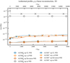 |
Fig. 1. Time evolution of the maximum Mach number in a 1D atmosphere with an isothermal temperature profile (Eq. (74)) and a linear gravitational potential (Eq. (73)). The colors indicate different well-balancing (WB) methods, the markers different flux functions. CL stands for Cargo–LeRoux. Time is given in units of the Brunt–Väisälä time tBV = 9.93 s (Eq. (18)) and sound-crossing time tSC = 3.10 s (Eq. (19)). The curves have been slightly smoothed for better visibility. |
Certain phenomena, such as convection, are inherently multidimensional and cannot develop in 1D geometry. Therefore we repeat this test using a two-dimensional (2D) atmosphere. For simplicity we keep gravity pointing in the negative x-direction. The horizontal boundaries are periodic. Figure 2 shows the evolution of the maximum Mach number and horizontal density fluctuation Δ𝜚 over time. The latter is defined as
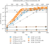 |
Fig. 2. Same as Fig. 1, but for a 2D atmosphere. The solid lines represent the maximum Mach numbers on the grid and the dotted lines the horizontal density fluctuations according to Eq. (75). The curves have been slightly smoothed for better visibility. |
with ⟨ ⋅ ⟩y denoting an average over the y direction.
Similar to the 1D case, we see that the simulations without well-balancing immediately reach Mach numbers around 10−5. All simulations using any well-balanced method start from very low Mach numbers (≈10−13), but the ones using the low Mach number AUSM+-up flux show an exponential growth over the next few thousand tBV. The growth of the Mach number is linked to that of Δ𝜚. This growth even affects the Mach numbers in the simulation without well-balancing, where the Mach number increases further after about 4000 tBV. The well-balanced simulations using the  flux do not show this behavior and retain the very low Mach numbers. We found that other low Mach number fluxes, such as the one by Miczek et al. (2015) and Li & Gu (2008), show a growth similar to AUSM+-up, although the rate varies between the different schemes. These spurious velocities are likely due to pressure–velocity decoupling, which is a common issue with compressible low Mach number methods. In combination with a gravity source term this can lead to an instability very similar to convection, but in stable stratifications. The reason is that pressure does not immediately return to its horizontal equilibrium. A common way to partially alleviate this effect is to introduce a form of pressure diffusion, such as the one suggested by Edwards & Liou (1998), which is also used in the AUSM+-up solver.
While the standard flux seems to perform better in this static test case, it is ultimately not suited for the simulation of dynamic phenomena at low Mach numbers, such as convection or waves, due to its high numerical dissipation.
Figure 3 shows the typical pattern of the exponentially growing perturbation in both Mach number and Δ𝜚. In both quantities we see a resolved pattern in the horizontal direction, but a grid-level oscillation in the vertical direction. One hypothesis for this behavior is that it is due to unresolved internal gravity waves in combination with pressure–velocity decoupling, see Sect. 5.3.
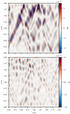 |
Fig. 3. Mach number (top panel) and horizontal density fluctuation Δ𝜚 (bottom panel) of the 2D isothermal simulation using the AUSM+-up flux and deviation well-balancing at time t = 1000 tBV. Gravity is directed in negative x-direction. |
We run the same tests for polytropic stratifications. Here the profiles of density, pressure, and temperature are
with
We set μ = 1 g mol−1. The polytropic index ν determines the slopes of the profiles. If ν is less than the adiabatic exponent γ, the atmosphere is stable. If ν > γ, it is unstable. If both are equal the atmosphere is isentropic and therefore marginally stable.
Figure 4 shows the maximum Mach number and Δ𝜚 for an isentropic atmosphere. Here the Brunt–Väisälä time tBV is not well defined because N = 0. Instead we use the sound-crossing time tSC = 4.28 s for reference. α-β and deviation well-balancing stay at very low Mach numbers below 10−7, independently of the choice of flux function. This result suggests that the issue with the exponential growth of perturbations in combination with low Mach number flux functions is more severe in more stable stratifications. In contrast to the isothermal test we see that Cargo–LeRoux well-balancing behaves quite similarly to the not well-balanced case. Both quickly reach Mach numbers of about 10−1 with flow patterns that resemble 2D convection. It is likely that this marginally unstable stratification experiences the growth of convection due to the less than ideal well-balancing properties of the Cargo–LeRoux method.
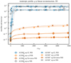 |
Fig. 4. Same as Fig. 2, but for an isentropic stratification. The solid lines represent the maximum Mach numbers on the grid and dotted lines the horizontal density fluctuations according to Eq. (75). Time is given in units of the sound-crossing time tSC = 4.28 s. The curves have been slightly smoothed for better visibility. |
As a last test we run a polytropic stratification with ν = 1.6 < γ = 5/3, which is stably stratified, but less so than the isothermal case. The relevant timescales here are tBV = 20.1 s and tSC = 4.13 s. The results are shown in Fig. 5. Here we see that the cases without well-balancing and with Cargo–LeRoux well-balancing fail to preserve the hydrostatic equilibrium in combination with the low Mach number flux. For the other two well-balancing methods there is a much clearer difference in the growth rate of the perturbation with deviation well-balancing growing significantly more slowly, reaching only Mach numbers of 10−7 after 5000 tBV. Any of the well-balancing methods manages to keep the Mach numbers below 10−11 when combined with the  flux, which does not have low Mach number properties. This is in agreement with the findings in the isothermal case.
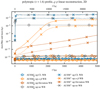 |
Fig. 5. Same as Fig. 2, but for a polytropic stratification with ν = 1.6. The adiabatic exponent is γ = 5/3. The solid lines represent the maximum Mach numbers on the grid and dotted lines the horizontal density fluctuations according to Eq. (75). Time is given in units of Brunt–Väisälä time tBV = 20.1 s and sound-crossing time tSC = 4.13 s. The curves have been slightly smoothed for better visibility. |
Appendix A shows the same isentropic and polytropic tests as in Figs. 4 and 5, but in the 1D case. In contrast to the 2D cases, the Mach numbers stay at low values for the runs using well-balancing also when using the AUSM+-up solver. This is consistent with the hypothesis that these velocities are a form of unphysical convection caused by pressure–velocity decoupling, which is obviously not possible in only one spatial dimension.
The spurious growth we found in combination with low-Mach-number fluxes is likely not a problem particular to the well-balanced methods we presented. We considered very long timescales of thousands of sound-crossing and Brunt–Väisälä times. This is much longer than the timescales typically used to test well-balancing methods. Käppeli & Mishra (2016), for example, ran their hydrostatic setup only for 2 tSC2. While this would definitely show any major issues with the basic well-balanced property of the scheme, it does not reveal the long-term growth of instabilities in the stable region. This is something to bear in mind when applying such methods to partly convectively stable configurations, such as stars. Whether the described phenomenon is an issue for real-world applications depends on many factors, such as how well the stratification is resolved and what timescales are of relevance. In particular for applications with large stable regions and long simulation times, such as in asteroseismological hydrodynamics simulations, this has to be carefully considered. The most promising method in this test is the deviation well-balancing method in combination with the AUSM+-up flux.
5.2. Hot bubble
Convection in the stellar interior is usually slow and almost adiabatic. A typical convection zone is nearly isentropic, although the stratification in the star’s gravitational field can span orders of magnitude in pressure and density. The buoyant acceleration of a fluid parcel is given by its entropy fluctuation with respect to the mean entropy at any given radius. Entropy fluctuations are constantly created by sources of heating or cooling. However, once the fluid parcel has left the heating or cooling layer and travels through the rest of the convection zone, the parcel’s entropy must be preserved except for those parts that have mixed with their surroundings. If the flow is slow, all entropy fluctuations inside the convection zone are also small and it becomes numerically challenging to preserve their exact values when density and pressure change by large factors as the fluctuations are advected along the gravity vector.
We test the numerical schemes’ entropy-preservation properties under the conditions described above by simulating the buoyant rise of a “bubble” with an adjustable initial entropy fluctuation embedded in a layer of constant entropy. The layer is strongly stratified in pressure and density due to the presence of gravity. We call this setup “hot bubble”, because we use positive initial entropy fluctuations. Negative initial entropy fluctuations would make the bubble fall, but everything else would work in the same way. Our setup is similar to that used by Almgren et al. (2006) to test their MAESTRO code, although their equation of state and stratification differ from our setup. We also test our methods down to much lower Mach numbers.
We construct the stratification in a two-dimensional box 106 cm wide and spanning the vertical range from y = 0 to y = ymax = 1.5 × 106 cm. To avoid any influence of boundary conditions, we use periodic boundaries and a periodic profile of gravitational acceleration
where g0 is a constant to be specified later and ky = 2π/ymax. The box is filled with an ideal gas with the ratio of specific heats γ = 5/3 and mean molecular weight μ = 1 g mol−1. At y = 0, we set the pressure to p0 = 106 Ba and the temperature to T0 = 300 K. The stratification is isentropic, that is
where A = A0 = const. everywhere outside of the bubble. Inside the bubble, we perturb the entropy via
![$$ \begin{aligned} A = A_0\left[1 + \left( \frac{\Delta A}{A} \right)_{t=0} \cos \left( \frac{\pi }{2} \frac{r}{r_0} \right)^2 \right], \end{aligned} $$](/articles/aa/full_html/2021/08/aa40653-21/aa40653-21-eq122.gif)
where (ΔA/A)t = 0 is the bubble’s amplitude and r = [(x−x0)2+(y−y0)2]1/2 is the distance from the bubble’s center with x0 = 5 × 105 cm and y0 = 1.875 × 105 cm. The bubble has a radius of r0 = 1.25 × 105 cm. We do not perturb the hydrostatic pressure stratification, which is given by the expression
![$$ \begin{aligned} p({ y}) = \left\{ p_0^{1 - \frac{1}{\gamma }} + \left(1 - \frac{1}{\gamma } \right) \frac{g_0}{A_0^{\frac{1}{\gamma }} k_{ y}} \left[ 1 - \cos (k_{ y} { y}) \right] \right\} ^{\frac{\gamma }{\gamma - 1}}. \end{aligned} $$](/articles/aa/full_html/2021/08/aa40653-21/aa40653-21-eq123.gif)
The amplitude g0 of the gravity profile sets the ratio of the maximum to the minimum pressure in the periodic pressure profile. To make the problem numerically challenging, we use a pressure ratio of 100, which is achieved with g0 = −1.09904373 × 105 cm s−2. This stratification is stronger than that in the convective core of a typical massive main-sequence star, in which the pressure changes by a factor of a few. On the other hand, the relative pressure drop from the bottom of the solar convective envelope to the photosphere is ≈109.
We start with a moderate initial entropy perturbation of (ΔA/A)t = 0 = 10−3, which makes the bubble rise at moderately low Mach numbers of a few times 10−2. This allows us to perform simulations with all three well-balancing methods as well as simulations without any well-balancing at modest grid resolution of 128 × 192, see Fig. 6. We run this series of simulations with fixed time steps of 0.2 s. With the exception of the Cargo–LeRoux and α-β methods, which require 𝜚-P reconstruction, we test both 𝜚-P and 𝜚-T reconstruction. The central, most buoyant, part of the bubble accelerates fastest. The bubble gets deformed into a mushroom-like shape with two trailing vortices and it expands as it rises into layers of lower pressure. Ideally, the initially positive entropy fluctuations ΔA/A should mix with the isentropic (ΔA/A = 0) background stratification, creating smaller but still positive entropy fluctuations. The entropy fluctuations may locally increase a bit as kinetic energy is slowly dissipated into heat, but there is no physical way for them to become negative. Any negative entropy fluctuations in the numerical solution result from numerical errors.
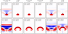 |
Fig. 6. Time evolution (top to bottom) of the hot-bubble problem when solved using different well-balancing and reconstruction schemes (left to right) on a 128 × 192 grid. In all of the cases, entropy fluctuations ΔA/A are shown on the same color scale ranging from −10−3 (dark blue) through 0 (white) to 10−3 (dark red). The minimum and maximum values of ΔA/A in the whole simulation box are given in each panel’s inset. The amplitude of the initial entropy perturbation is (ΔA/A)t = 0 = 10−3. |
Figure 6 shows that both the absence of well-balancing and the Cargo–LeRoux method generate large areas of negative entropy fluctuations comparable to or even larger in absolute value than the bubble’s initial amplitude. Large-scale positive entropy fluctuations also occur far from the bubble and they clearly do not result from hydrodynamic mixing. They rather seem to be caused by entropy nonconservation as the bubble pushes the surrounding stratification upwards and downwards. In the no-well-balancing case, errors in ΔA/A are smaller when 𝜚-T reconstruction is employed as compared with 𝜚-p reconstruction. This may be due to the fact that the pressure changes by a factor of 100 in the computational domain whereas the temperature only changes by a factor of 6.3. In any case, α-β and deviation well-balancing clearly provide far superior results with only a mild and highly localized undershoot in ΔA/A above the bubble. With the deviation method, this success is independent of the choice of reconstruction.
All of the methods tested converge upon grid refinement, although not in the same way, see the series of runs shown in Fig. 7. In this series, we keep the 0.2 s time steps for all runs except those on the finest (256 × 384) grid, for which we use 0.1 s. When there is no well-balancing or the Cargo–LeRoux method is used, the amplitude of the large-scale entropy-conservation errors around the bubble decreases upon grid refinement and the bubble’s shape slowly approaches that obtained with the α-β and deviation methods. The errors are still substantial even on the finest (256 × 384) grid tested. The slight entropy undershoot produced by the α-β and deviation methods does not decrease in amplitude but it does decrease in spatial extent as the grid is refined. Surprisingly, we do not observe any significant entropy fluctuations far from the bubble even on the coarsest grid (64 × 96) with these two methods.
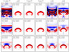 |
Fig. 7. Same as Fig. 6, but showing the solutions’ resolution dependence (top to bottom) at t = 300 s. |
As the bubble’s initial amplitude (ΔA/A)t = 0 is decreased, the typical Mach number in the flow field decreases as
This scaling results from the fact that the bubble’s acceleration is proportional to Δ𝜚/𝜚∝ΔA/A and the velocity an object in uniformly accelerated motion reaches over a fixed distance (i.e., until the bubble has reached the same evolutionary stage) is proportional to the square root of the acceleration. Although the bubble’s acceleration is not constant, the bubble always evolves in the same way, just slower, when its initial amplitude is decreased and the scaling still holds.
The scaling is also demonstrated in Fig. 8, which shows a series of runs performed on a 128 × 192 grid with (ΔA/A)t = 0 ranging from 10−3 down to 10−11. As (ΔA/A)t = 0 decreases, we increase time steps in this order: 0.2 s, 1 s, 10 s, 25 s, 25 s. The solver’s convergence worsens as all fluctuations become smaller, limiting the maximum time step size. We only include the α-β and deviation well-balancing methods in this experiment, because entropy-conservation errors quickly dominate the solution when the initial amplitude is decreased and the Cargo–LeRoux or no well-balancing method is used. Because the Mach number is expected to scale according to Eq. (82), we scale the time when the simulation is stopped with  . This way, we compare the results when the bubble has reached approximately the same height and evolutionary stage as the previously discussed case with (ΔA/A)t = 0 = 10−3 at t = 300 s (Fig. 6). Both the α-β and deviation well-balancing methods provide essentially the same solutions, reproducing the expected Mach-number scaling down to Ma ∼ 10−6. The amplitude of the entropy undershoot above the bubble is 24% lower when the α-β method is used as compared with the deviation method. The most extreme run with (ΔA/A)t = 0 = 10−11 reaches the limits of our current implementation and we can see numerical noise developing in the stratification, see Figs. B.1 and B.2. Figure 8 also shows that the minimum and maximum entropy fluctuations in the evolved flow scale in proportion to the initial amplitude of the bubble.
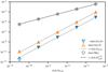 |
Fig. 8. Dependence of the maximum Mach number Ma and minimum and maximum entropy fluctuations ΔA/A on the bubble’s initial amplitude (ΔA/A)t = 0. All measurements are taken when the bubble has evolved to a stage comparable to that shown in the bottom row of Fig. 6. Open and filled symbols correspond to runs with α-β and deviation well-balancing, respectively. The lines show that the Mach number scales according to Eq. (82) and the minimum and maximum entropy fluctuations scale in proportion to the bubble’s initial amplitude. |
5.3. Simple convection setup
The previous section demonstrated the capabilities of the α-β and deviation well-balancing schemes to evolve the rise of a bubble with an entropy excess in an isentropic stratification at low Mach numbers. This can be interpreted as a test for the fundamental mechanism of convection. The purpose of this section is to also assess the benefit from well-balancing techniques for fully developed convection in a realistic stellar scenario.
The prototype of a convective region in stellar interiors includes a steady heating source in the form of nuclear burning that injects energy over a long period in time. If radiative transport of energy is not efficient enough, the temperature gradient will steepen until it reaches the adiabatic temperature gradient. According to Eq. (16), this region will become unstable and convection will set in. As convection is very efficient in transporting energy, a common assumption is that the stratification settles to an nearly adiabatic temperature gradient in the steady state.
In stars, a convective region is typically adjacent to convectively stable regions. The mixing processes across the interfaces of convectively stable and unstable regions have a profound impact on stellar evolution, yet it is particularly difficult to parametrize these processes in one-dimensional stellar evolution codes. A common strategy for improving the current 1D description is to investigate the dynamics at the interfaces of convection zones by means of multidimensional hydrodynamical simulations (Jones et al. 2017; Cristini et al. 2019; Pratt et al. 2020; Higl et al. 2021; Horst et al. 2021).
The Mach number of convection deep in the stellar interior is estimated to be on the order of 10−4 in early stages of stellar evolution. Accurate modeling of the early phases is, however, crucial as it determines the whole subsequent evolution of the star and inaccuracies will propagate to later stages. Thus, numerical experiments that address convection in stellar interiors rely on schemes that accurately maintain hydrostatic stratifications and that are able to follow convection at low Mach numbers for a sufficient amount of time.
The initial stratification for the test series presented in this section consists of a convective region with a stable layer on top. One possibility to set up this configuration would be to use realistic initial conditions from a 1D stellar evolution code. However, such 1D profiles usually require some extra treatment before they can be used for hydrodynamical simulations, for example a smoothing of sharp composition gradients or to properly impose a flat entropy profile in the convection zone. Instead, we use analytical initial conditions to be able to test the numerical methods under well-defined but realistic conditions. This way, any numerical artifacts that may arise can solely be attributed to the methods applied rather than to inadequate initial conditions.
To construct the initial hydrostatic stratification, we follow the procedure described by Edelmann et al. (2017). It imposes the profile of the superadiabaticity Δ∇ = ∇ − ∇ad while integrating the equation of hydrostatic equilibrium (Eq. (11)). According to Eq. (16), Δ∇ determines the sign of the Brunt–Väisälä frequency. It is therefore possible to precisely control which regions are convectively stable (Δ∇ < 0) and unstable (Δ∇ > 0) as well as the respective transitions between these regions. A marginally stable stratification is imposed inside the convection zone by setting Δ∇CZ = 0. In the stable region, we impose Δ∇SZ = −∇ad, which corresponds to an isothermal stratification.
To connect the two regions, we use a sinusoidal transition, which ensures that the transition between the two Δ∇-values is well-defined and can be resolved numerically. The profile with a transition between the convection and stable zones then takes the form
![$$ \begin{aligned} \Delta \nabla ({ y})&= \Delta \nabla _{\mathrm{CZ}} \nonumber \\&+ \frac{1}{2}\left[1 + \sin \left(\frac{\pi }{2}\,\eta ({ y}, K, { y}_{\mathrm{\mathrm{CZ},\mathrm{SZ}}})\right)\right]\left(\Delta \nabla _{\mathrm{SZ}}-\Delta \nabla _{\mathrm{CZ}}\right), \end{aligned} $$](/articles/aa/full_html/2021/08/aa40653-21/aa40653-21-eq126.gif)
with
where the constant K determines the steepness of the transition. It is set such that the transition is resolved by at least 20 grid cells. The coordinate yCZ, SZ denotes the middle of the transition starting at yCZ, SZ − 1/K and ending at yCZ, SZ + 1/K. The value of yCZ, SZ is given in Table 2. The computational domain spans 2yCZ, SZ in the horizontal direction. The profiles of temperature T, pressure p and density 𝜚 then follow from integrating the equation of hydrostatic equilibrium Eq. (11) as described by Edelmann et al. (2017) with a spatially constant gravitational acceleration of |g| = 6.6 × 104 cm s−2. The initial values required for the integration are listed in Table 2. They are representative of the conditions expected in the convective core of a 25 M⊙ main sequence star with a mean atomic weight of  and a mean charge of
  .
.
Parameters of the convection test setup.
Figure 9 shows the resulting profiles of Δ∇, T, and 𝜚 as well as the fact that the transition between the convective and stable zone is well resolved even on the coarsest SLH grid. Because cores of massive stars are hot, a considerable fraction of the total pressure is contributed by the radiation field. The relative importance of radiation pressure is given in the lower panel of Fig. 9. It ranges from roughly 20% in the bottom region to about 60% in the top region where the density is low. This test setup is therefore also an example where the ideal gas EoS is not sufficient to describe the thermodynamic behavior of the gas and which requires well-balancing methods that can handle general EoS.
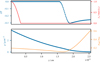 |
Fig. 9. Initial stratification of the convection setup. The red curve illustrates the position and shape of the energy injection which has nonzero values only at the bottom of the convection zone. Its actual amplitude is set for the different simulations individually. Dots denote the positions of cell centers on a grid with 144 vertical cells, the lowest resolution used in the SLH simulations presented in this section. |
To trigger convection in the initially marginally stable convection zone, a heat source is placed at the bottom of the convection zone that continuously injects energy into the system with a sinusoidal profile peaking at the bottom of the domain. The heating profile is given by
![$$ \begin{aligned} \dot{e}_h({ y}) = {\dot{e}_0}\,a\, \sin \left(\frac{\pi }{2}\left[1+\eta \left({ y}, K, 0\right)\right]\right)\,\mathrm{erg}\,\mathrm{s}^{-1}\,\mathrm{cm}^{-3}, \end{aligned} $$](/articles/aa/full_html/2021/08/aa40653-21/aa40653-21-eq131.gif)
with
where Δy denotes the grid spacing in the vertical direction. As introduced here, ė0 is dimensionless. The factor a ensures that the total heating rate is independent of grid resolution. In a stationary state, the convective velocity is expected to scale with the heating rate,
This scaling can be motivated using dimensional arguments (e.g., see Jones et al. 2017) or the mixing-length theory (Kippenhahn et al. 2012) and has been confirmed in numerical experiments (e.g., Cristini et al. 2019; Edelmann et al. 2019; Andrassy et al. 2020).
To test the low-Mach capabilities of the methods that are presented in this paper, the amplitude of the heating factor ė0 is decreased successively while the root mean square (rms) Mach number measured from the simulation is compared to the expected scaling Eq. (87). The upper limit of ė0 is chosen such that the resulting Mach number is in a regime where also simulations without well-balancing follow the scaling. A deviation from the expected scaling at lower values of ė0 and correspondingly lower Mach number then indicates that numerical errors have become significant and the method has reached its limit of applicability. The scaling test is performed for all available well-balancing methods and also in the absence of well-balancing. The domain is discretized by 72 × 144 cells. This rather coarse resolution is chosen to assess the ability of the well-balancing method to balance hydrostatic stratifications even with a moderate number of cells. While any consistent method will ultimately be able to follow low-Mach-number flows given a sufficiently fine grid, this is computationally not feasible, especially in 3D. The simulations use periodic boundary conditions in the horizontal direction. At the top and bottom of the domain solid-wall boundaries are employed that do not allow mass to enter or leave the domain. For the time stepping, we set cCFL = 0.5. The initial stratification is perturbed by random density fluctuations at the 𝒪(10−14) level to facilitate the growth of the convective instability. Additionally, the heating profile Eq. (85) is modulated by a sinusoidal function along the horizontal direction to break the initial horizontal symmetry. The wavelength is one fourth of the horizontal extent and the amplitude is set to 0.01 ėh(y). The modulation is switched off after the flow has reached a substantial fraction of its final speed.
For all simulations, a grid file is saved every 200 time steps. For each saved grid, the mass-weighted rms Mach number Marms is calculated. To this end, only the fixed region from ybot to yCZ, SZ is considered, although the position of the boundary between convective and stable zone is dynamical and may change over time. However, for the simulation presented in this section, this effect is negligible and a fixed region is chosen for convenience. For all simulations, Marms is then averaged over the same time span in terms of the convective turnover time τconv, which we define as
where vrms is the rms velocity. This ensures that the stochastic fluctuations, which have different typical timescales for different flow speeds, are accounted for in a similar way for all simulations. Due to the steady heat injection and the small amount of numerical dissipation in 2D simulations, the value of τconv slightly decreases over time as velocities slightly increase. Thus, the average of τconv depends on the time interval considered and is not clear how to chose the proper time interval for the different simulations. Instead, the number of turnover times Nτ as a function of physical time t,
is used to determine the respective time intervals and the averaging is done in the time interval t ∈ [t(Nτ = 5), t(Nτ = 10)]. The resulting Marms as functions of the heating rate are depicted in Fig. 10. For the two highest values of ė0, that is at Marms around 9 × 10⁻³ and 4 × 10⁻³, all methods agree and Marms follows the scaling given by Eq. (87). This is not the case at lower heating rates. For ė0 ≲ 105, the simulation using the Cargo–LeRoux well-balancing method considerably deviates from the expected scaling by giving a value of Marms that does not correlate with the energy input anymore but stays rather constantly slightly below 4 × 10⁻³. Almost identical results are found when no well-balancing is applied in combination with 𝜚-p as reconstruction variables. At this point, it seems that Cargo–LeRoux well-balancing is not able to improve the behavior at lower Mach numbers. The results slightly improve if 𝜚-T are used for reconstruction and no well-balancing is used. In this case, the Mach number settles slightly below Marms = 2 × 10⁻³ for an energy input rate lower than ė0 = 105. The reason for this could be the nonnegligible contribution of radiation-pressure to total pressure. As prad ∝ T4, a more accurate reconstruction of T could lead to an interface pressure that is closer to the hydrostatic solution and hence artifacts from imperfect balancing are reduced.
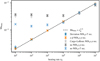 |
Fig. 10. Root mean square Mach number Marms as a function of the heating rate ė0. The dashed line represents the expected scaling according to Eq. (87). All values correspond to time averages over t ∈ [t(Nτ = 5), t(Nτ = 10)] (see text). The vertical error bars denote one standard deviation of the temporal average of Marms. |
By definition, α-β well-balancing requires 𝜚-p to be reconstructed while the variables can be chosen freely for deviation well-balancing. Hence we have chosen 𝜚-T for the deviation runs for comparison. However, no major differences can be seen between α-β and deviation in Fig. 10. Both Marms profiles closely follow the scaling down to the smallest value of ė0. Due to the hydrostatic solution’s being stored at cell interfaces in these two methods, the particular choice of variables for reconstruction seem to be less important. In contrast, the Cargo–LeRoux method reconstructs the potential q at the interfaces using values at the cell centers, which can introduce an error in the total energy over many time steps. A possible fix for this would be to store q at the cell interfaces, however this is currently not implemented in our code.
It is not obvious how to assess the accuracy at which hydrostatic equilibrium is maintained within the convective region. Convection will inevitably introduce ram pressure, pram. Its ratio with thermal pressure, pthermal, is expected to scale as  . This gives an order-of-magnitude estimate for the expected minimal deviation from the initial hydrostatic pressure stratification caused by convective motion alone, independent of the choice of well-balanced method. We have verified that the respective relative deviation from the hydrostatic pressure at t(Nτ = 7.5) scales as
  for all sets of simulations. The only exception is the simulation with deviation well-balancing at the lowest heating rate, which may be a result of sound waves excited by the strong flow field in the stable zone (see Fig. 11 and the next paragraph). Table C.1 lists the ratio exemplarily for the simulations using α-β well-balancing. There, the relative deviation ranges from about 10−7 at the smallest heating rate to roughly 10−4 at the largest rate. At t = 0 we measure a mean relative deviation of 2.7 × 10⁻⁸, which originates entirely in the discretization error of the pressure gradient. The fact that the relative deviations from hydrostatic equilibrium are of the same order of magnitude as the ram pressure implies that they are not an artifact of the well-balancing method, but physically caused by the convective motions.
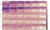 |
Fig. 11. Mach number of the flow for different values of the heating rate ė0 (left to right) and different well-balancing methods (top to bottom). The dashed black lines denote the boundaries of the convection zone at y = ytop, see Table 2 for an overview of simulation parameters. The insets displays the rms Mach number Marms within the convection zone for the snapshot shown. All snapshots are taken at t(Nτ = 7.5). |
To also add a qualitative visual verification of the arising convection, the flow patterns are shown in Fig. 11 in the middle of the time frame considered. For the highest heating rate, all simulations show the typical flow morphology of two-dimensional convection: A pair of large eddies form with a size that is determined by the vertical extent of the convection zone. At lower heating rates, the flow pattern remains basically the same for deviation and α-β well-balancing, which strengthens our confidence in these solutions. In contrast, the flow patterns obtained with Cargo–LeRoux well-balancing or without any well-balancing are dominated by incoherent, small-scale structures. While for the “no WB” run with 𝜚-T reconstruction, the Mach numbers achieved are somewhat smaller, the general flow pattern is similar. We assume that these motions are caused by the imperfect hydrostatic equilibrium.
Convective regions are known to excite internal gravity waves (IGW) in adjacent stable layers (see e.g., Rogers et al. 2013; Edelmann et al. 2019; Horst et al. 2020). Assuming that IGW are predominantly generated at periods close to the convective turnover time τconv (cf. Edelmann et al. 2019), we can estimate their vertical wavelength λv using the dispersion relation of IGW in the Boussinesq approximation (see, e.g., Sutherland 2010),
![$$ \begin{aligned} \lambda _\mathrm{v} = \frac{\lambda _\mathrm{h} }{\sqrt{\left[{N {\tau _{\rm conv}}}/({2\pi })\right]^2 -1 }}, \end{aligned} $$](/articles/aa/full_html/2021/08/aa40653-21/aa40653-21-eq138.gif)
where λh is the horizontal wavelength. It follows that the vertical wavelength decreases with increasing τconv for λh = const. and the waves will become unresolved when the heating rate is decreased on the same computational grid.
We estimate the vertical wavelengths according to Eq. (90) exemplarily for the simulations with deviation well-balancing shown in Figs. 10 and 11. To calculate λv, the value of the Brunt–Väisälä frequency is taken at the top of the box domain and λh = 2 yCZ, SZ, which corresponds to the maximal horizontal wavelength that fits into the computational domain. The ratio of λv to the vertical grid spacing is shown in Fig. 12 as black crosses. At all but the two highest heating rates, the vertical wavelength is less than two cells and it follows from the Nyquist sampling criterion that such waves cannot be represented on our coarse grid. Indeed, for these runs strange patterns appear in the stable zone as can be seen in Fig. 11. A peculiar pattern is visible in the stable zone for deviation well-balancing at the lowest heating rate. While its origin is not completely understood, we have verified that the results look similar to the other runs when 𝜚-p reconstruction or a higher grid resolution is applied. Our estimate gives typical wavelengths of two to six cells in the two simulations with the highest heating rates. Hence, the flow patterns in Fig. 11 for these two simulation probably include some real internal gravity waves, but they are still dominated by artifacts.
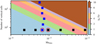 |
Fig. 12. Expected typical vertical wavelength (Eq. (90)) in grid cells of internal gravity waves as a function of Marms in two series of simulations with the deviation well-balancing method. Black crosses correspond to simulations at fixed resolution but increasing heating rate. Blue crosses correspond to simulations at a fixed heating rate but different resolution. The two encircled data points result from the same simulation but Marms has been determined at a different time. |
To confirm that our interpretation is correct, we run another series of simulations with increasing vertical resolution at ė0 = 104. Deviation well-balancing is used in this experiment. Because of the higher computational costs, there is not enough data to perform meaningful averages and Marms is extracted for a single snapshot as soon as convection has developed in the whole convective zone. The results are shown as blue crosses in Fig. 12. Because Marms is measured at earlier times compared with the corresponding simulation in the heating series, the Marms of the lowest-resolution run does not coincide with the (red circled) black cross corresponding to the same simulation. We see that the expected typical vertical wavelength is resolved by more than eight cells on the finest grid. Figure 13 shows the flow pattern for the different grid resolutions. In the center and right panel of the lower row, the resolution in the convective zone corresponds to the resolution of the upper right panel (288 × 576). Close to the transition to the stable zone, the vertical spacing is smoothly reduced to 1/32 of the starting resolution. This saves computing resources and also illustrates that the patterns do not depend on the resolution in the convective zone. The transition is shown in Fig. C.1.
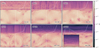 |
Fig. 13. Mach number for a heating rate of ė0 = 104 and deviation well-balancing at different resolutions. The upper left box in each panel indicates the change in the vertical resolution relative to the resolution used for the Mach number scaling. The lower right box gives the total number of cells of the particular simulation. All snapshots are taken as soon as convection has fully developed. The dashed white line illustrates the profile of the Brunt–Väisälä frequency as a function of height with arbitrary units on the x-axis. |
Our resolution study indicates that with increasing vertical resolution in the stable zone artifacts are diminished. For the highest resolution fine wave patterns are observed. As grid resolution increases, nearly horizontal wave patterns first appear close to the convective boundary, where N gradually increases from zero to relatively large values higher up in the stable zone.
While our findings can be explained by unresolved IGW, we cannot exclude that at least to some extent also numerical artifacts contribute to the flows in the stable zone. Nevertheless, our tests with the simple convective box show that, as soon as we resolve the IGW sufficiently, artifacts tend to disappear and any instabilities possibly still present do not visibly dominate the flow. At the same time, this illustrates that, depending on the actual stellar profile, rather high grid resolution is needed to properly resolve the waves.
5.4. Keplerian disk
Some astrophysical problems involve stationary solutions that are not at rest, for example a rotating star that is partially stabilized by the centrifugal force (e.g., Tassoul 2000; Maeder 2009). Another case is the Keplerian motion around a central gravitational mass m in its gravitational potential  . Gaburro et al. (2018) describe a nondimensional test setup of a circular disk with 𝜚0 = p0 = 1 around a massive object. Neglecting its own gravitational field, such a disk can be stabilized by a flow velocity of
![$$ \begin{aligned} u(x,{ y}) =&- \sin \left[\mathrm{atan2} \left({ y}, x\right)\right] \root \of {\frac{Gm}{r(x,{ y})}} \end{aligned} $$](/articles/aa/full_html/2021/08/aa40653-21/aa40653-21-eq140.gif)
![$$ \begin{aligned} { v}(x,{ y}) =&\cos \left[\mathrm{atan2} \left({ y}, x\right)\right] \root \of {\frac{Gm}{r(x,{ y})}}, \end{aligned} $$](/articles/aa/full_html/2021/08/aa40653-21/aa40653-21-eq141.gif)
where  and atan2(y,x) is the typical shortcut for choosing the quadrant of arctan(y/x) correctly. For convenience we set G = m = 1. We simulate the Keplerian disk from radius r = 1 to 2 on a polar grid with 20 radial and 70 angular cells as well as on a finer grid with 100 radial and 350 angular cells. Polar coordinates are the appropriate choice for the problem’s geometry and should therefore lead to the least amount of numerical errors. We use periodic and solid-wall boundaries in the angular and radial directions, respectively. The flow has a maximum Mach number of 1 at the inner domain boundary dropping to ≈0.6 at the outer boundary. We perform most of our simulations with the explicit RK3 scheme (see Sect. 3) because it is more efficient in this Mach number range. The time step of explicit runs is set by the CFLuc criterion (Eq. (28)) with cCFL = 0.4. For the lower-resolution setup we also perform simulations with implicit time stepping and the CFLug time step criterion (Eq. (26)) with cCFL = 0.4. We find that the results of the implicit runs are identical to the explicit time stepping (see dots in upper panel of Fig. 14). Tests with the explicit, second-order RK2 scheme also give almost identical results.
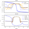 |
Fig. 14. Time evolution of the angle-averaged density profiles |

Since the disk is isobaric, we use 𝜚-p reconstruction for this test case. Here we only compare simulations without well-balancing to runs with deviation well-balancing, since the other methods presented in this work are not capable of stabilizing a target solution with a nonzero velocity field (see Sect. 4.3).
In order to asses the stability of the setup we add a density perturbation with 𝜚 = 2 in the circular region (x + 1.5)2 + y2 < 0.152 and follow its evolution up to 10 000 orbital periods, where the orbital period is taken at the central point of the perturbation. A perfect solution will maintain the initial radial density distribution of the perturbation at all times. However, due to its radial extent there will be a phase shift between the innermost and outermost regions of the perturbation. Furthermore, numerical diffusion will spread the perturbation predominantly in the direction of its movement. Therefore the perturbation evolves into a homogeneous ring orbiting the central object with a density that corresponds to the initial angle-averaged density  .
.
In Fig. 14 we show how the profile of  evolves with time. The target solution is given as a black dashed line. For a grid resolution of 20 × 70 cells the run without well-balancing only shows small deviations from the target solution after 10 orbital periods. However, we already see that mass starts to accumulate in the center. The mass can not leave the domain and accrete onto the central object due to our wall boundaries. Over time, more and more mass flows to the inner boundary. After 100 orbits the center has approximately the same density as the initial perturbation, and after 1000 orbits the profile has completely shifted toward the inner boundary. This is also clearly visible in the two-dimensional density distribution shown in Fig. D.1. With deviation well-balancing the profile remains mostly stable up to 1000 orbits. The perturbation is slowly diffusing symmetrically around the initial peak, maintaining the general shape of the initial density profile. After 10 000 orbits we see that also the run with deviation well-balancing has become noticeably asymmetric toward the center. The regions where the density falls bellow the initial density profile are most likely related to the fact that we do not use flux limiters for these runs. Undershoots at steep gradients are a common consequence of this omission.
Increasing the resolution improves the stability of the runs without well-balancing (see bottom panel in Fig. 14). At a resolution of 100 × 350 cells the distribution is still almost identical to the initial perturbation even after 100 orbits. Only after 1000 orbits we start to notice the accumulation of mass at the inner boundary similar to the low-resolution case. After 10 000 orbits, however, the distribution has again completely shifted towards the center and the initial perturbation is not recognizable any longer. The high-resolution run with deviation well-balancing, on the other hand, is almost identical to the target solution even after 1000 orbits. The increased radial resolution has reduced the radial diffusion observed in the low-resolution runs. The density undershoots become more noticeable at the 10 000 orbit mark. There we again identify a tendency for a slow drift towards the center. However, thanks to the use of well-balancing the shape of the initial perturbation is still retained approximately.
This test shows that the flexibility of the deviation well-balancing method also allows to maintain stable configurations other than hydrostatic equilibrium. This is particularly important for the long-term evolution of such systems. Without well-balancing stability can only be achieved by increasing grid resolution, which leads to substantially higher computational cost.
6. Summary and conclusions
We have presented the deviation, the α-β, and the Cargo–LeRoux well-balancing methods that aim to improve the ability of finite-volume codes to maintain hydrostatic stratifications even at moderate grid resolution. The performance of these methods were assessed in a set of test simulations of static and dynamical setups. Special emphasis was given to flows at low Mach numbers. They are particularly challenging to evolve because they require special low-Mach hydrodynamic flux solvers, which in turn come with reduced dissipation and hence are prone to numerical instabilities. Also, it seems natural that slight deviations from hydrostatic equilibrium lead to low-Mach flows, as is the case, for example, in stellar convection. All simulations were performed with the time-implicit SLH code that solves the fully compressible Euler equations using a modified version of the low-Mach AUSM+-up hydrodynamic flux solver. Our experience shows that the inclusion of gravitational potential energy in the total energy is essential to correctly representing slow flows in stratified atmospheres in the cell-centered discretization of gravity implemented in SLH; see Mullen et al. (2021) for an alternative approach. To the best of our knowledge, the present study is the first to reach Mach numbers as low as 2 × 10⁻⁴ in stratified convection using the fully compressible Euler equations.
The first test of the well-balancing schemes is to evolve a 1D hydrostatic atmosphere in time at low resolution for an isothermal, an isentropic, and a polytropic stratification. In all cases, the absence of a well-balancing scheme quickly led to spurious velocities at significant amplitudes. The application of any of the considered well-balancing methods removed this problem and managed to keep the flow below Mach numbers of 10−12 for very long times. Repeating the same test in 2D revealed that low Mach number flux functions, such as AUSM+-up, are subject to an exponential growth of the Mach number and horizontal density fluctuations, which is not physically expected in a stably stratified atmosphere. This effect became less pronounced the closer the stratification was to the marginally stable, isentropic profile. In the isentropic case α-β and deviation well-balancing in combination with the low-Mach flux remained stable (Ma ≲ 10−8) for long times, while with Cargo–LeRoux well-balancing the setup developed a flow at Mach numbers of about 10−1. These examples showed that it is important to test well-balanced schemes in more than one spatial dimension and for more than just a few sound-crossing times, as only then slowly growing instabilities become noticeable, especially in very stable stratifications.
While it is a necessary condition to maintain an initially static setup, only dynamical setups are of actual interest in multidimensional simulations. In a second test, we considered the rise of a hot bubble in a periodic background stratification spanning two orders of magnitude in pressure at constant entropy. We tuned the bubble’s entropy excess to reach different rising speeds. With Cargo–LeRoux well-balancing and without any well-balancing, unphysical entropy fluctuations appeared in large parts of the atmosphere and a relatively fine grid (256 × 384) was required to make their amplitude smaller than that of even the hottest bubble considered. The corresponding Mach number of Ma ∼ 3 × 10⁻² seemed to be close to a limit of practical applicability of these two methods in such a strong stratification. The α-β and deviation methods fared much better with no entropy changes far from the bubble and only a slight entropy undershoot right above the bubble even on a coarse (64 × 96) grid. Equally good results were obtained with the initial amplitude decreased by a factor of 106, leading to Ma ∼ 3 × 10⁻⁵. Numerical effects started to dominate only at Ma ∼ 3 × 10⁻⁶ after the amplitude was decreased by another factor of 102.
We proceeded with a setup involving a convection zone with a stable zone on top. The stratification was chosen to be representative of core convection in a 25 M⊙ main-sequence star. Radiation pressure was a substantial fraction of the total pressure, testing the methods’ capability to deal with a general EoS. We used volume heating of adjustable amplitude to drive the convection. With Cargo–LeRoux well-balancing and without well-balancing, the rms Mach number of the convective flow ceased to correlate with the heating rate at Marms ∼ 4 × 10⁻³ and the flow became dominated by small-scale structures of numerical origin. The lowest reachable value of Marms dropped by about a factor of two when switching from 𝜚-p to 𝜚-T reconstruction in the absence of well-balancing. Only the α-β and deviation methods were able to reproduce the expected scaling of Marms with the heating rate (Eq. (87)) down to the slowest flows tested (Marms ∼ 2 × 10⁻⁴). We observed spurious patterns in the stable layer and demonstrated that they were caused by unresolved internal gravity waves, whose vertical wavelength becomes extremely short with increasing period. The patterns disappeared when the typical vertical wavelengths of waves with periods close to the convective turnover frequency became resolved by 8 to 10 cells (grid of 288 × 2380 cells).
The deviation method, unlike the other methods presented in this work, can deal with arbitrary stationary states. We illustrated this capability in our last test, in which we followed many orbits of a density perturbation in a Keplerian disk around a point mass. The angle-averaged density profile should ideally remain constant in this model. Without any well-balancing, imperfect balance between the centrifugal force and gravity led to mass redistribution towards inner parts of the disk after many orbits. Deviation well-balancing much improved the solutions with only slight radial broadening of the initial perturbation even after 104 orbits with a moderate resolution of 100 × 350 cells.
In summary, our results show that well-balancing can substantially reduce the grid resolution needed to correctly follow tiny perturbations in situations in which the stationary background state involves the balance of two large opposing forces. We obtained comparable results with the α-β and deviation methods, both far surpassing the Cargo–LeRoux method in accuracy in the low-Mach-number regime. The α-β and deviation methods are also expected to be more accurate than the majority of other well-balanced methods present in astrophysical literature (e.g., Zingale et al. 2002; Perego et al. 2016; Käppeli et al. 2011; Käppeli & Mishra 2016; Padioleau et al. 2019), because they exactly balance the stationary solution rather than an approximation to it. Although an analytical prescription is often not available, the stationary solution can be computed to an arbitrary degree of accuracy in many astrophysical applications. This statement only holds in the case that the hydrostatic background state does not change in time. In this case an update is necessary, which we do not discuss in this paper. This step would likely involve a local approximation to hydrostatic equilibrium, similar to the ones suggested in the other aforementioned methods. It should be noted, however, that such an update is unnecessary in the case of very slow flows, such as in earlier phases of stellar evolution, because the background state hardly changes over time, even after hundreds of convective turnover times.
We prefer to use the deviation method, because it is more general and does not impose any restrictions on reconstruction variables. The method can be applied both to nearly hydrostatic cases and to cases in which rotation becomes important. The latter can have strong impact on stellar evolution (Maeder & Meynet 2000) as well as on the propagation of IGW in stars (Rogers et al. 2013).
The Cargo–LeRoux method still has its place, though. Horst et al. (2021) show for the case of convective helium-shell burning that this method considerably reduces numerical diffusion of the hydrostatic background stratification as compared to the unbalanced case if the gravitational energy is not included in the total energy. Therefore we consider the Cargo–LeRoux method as a valid method that leads to improvements already with little development effort.
This paper focuses on setups with simple grid geometries, but the SLH code can use general curvilinear grids. This allows us to adapt grid geometry to the problem at hand. Standard spherical grids adapt to the geometry of slowly or nonrotating stars, but they suffer from singularities at the center and at the poles. A star can be inscribed in a simple Cartesian grid (e.g., Woodward et al. 2015), but this requires to also impose a spherical boundary condition on the grid. When done on the cell level, the sphere is rough on small scales and can generate spurious vorticity. We have implemented the cubed-sphere grid proposed by Calhoun et al. (2008) in our SLH code. The grid is logically rectangular but geometrically spherical with a smooth outer boundary, see Fig. 15 for a 2D version. Discretization errors along the grid’s strongly deformed diagonals make it almost impossible to follow nearly hydrostatic flows without any well-balancing method. Figure 15 shows an SLH simulation with a convective shell embedded between two stably stratified zones. With deviation well-balancing, we obtain the expected convective shell with convection-generated IGW propagating in the stable zones. If we turn the well-balancing off, a convection-like flow of numerical origin appears and mixes the convection zone with the whole inner stable zone. This result is promising, but limits of applicability of the deviation method on the cubed-sphere grid are still to be investigated.
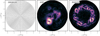 |
Fig. 15. Left panel: geometry of the cubed-sphere grid. The number of cells has been reduced compared to grids used in the other two panels to ease the identification of individual cells and their shapes. Middle and right panel: shell convection in a setup comparable to that in Sect. 5.3 but with a shallower stratification and ideal gas EoS. Middle panel: color coded Mach number in a run without well-balancing. Numerical discretization errors quickly lead to spurious flows in the central region and the maximum Mach number reaches 3 × 10⁻². In the run with deviation well-balancing shown in the right panel the convective shell is clearly maintained. The maximum Mach number is 2 × 10⁻³. |
Käppeli & Mishra (2016) show another test of a 3D simulation that covers several convective turnover times and contains a stable layer. The simulation shows strong, unphysical flows in the stable layer when run without a well-balanced method, but these disappear when their well-balanced method is used. Considering they did not use a low Mach number method, this is consistent with our results.
Acknowledgments
PVFE was supported by the U.S. Department of Energy through the Los Alamos National Laboratory (LANL). LANL is operated by Triad National Security, LLC, for the National Nuclear Security Administration of the U.S. Department of Energy (Contract No. 89233218CNA000001). PVFE, LH, JPB, RA, JH, GL, and FKR acknowledge support by the Klaus Tschira Foundation. The work of FKR and PVFE was supported by the German Research Foundation (DFG) through the graduate school on “Theoretical Astrophysics and Particle Physics” (GRK 1147). The work of CK and FKR is supported by DFG through grants KL 566/22-1 and RO 3676/3-1, respectively. JPB acknowledges the grants HITS 21.03.2018, HITS 18.12.2018 and HITS 26.08.2020. This work has been assigned a document release number LA-UR-21-21056.
References
- Almgren, A. S., Bell, J. B., Rendleman, C. A., & Zingale, M. 2006, ApJ, 637, 922 [Google Scholar]
- Andrassy, R., Herwig, F., Woodward, P., & Ritter, C. 2020, MNRAS, 491, 972 [Google Scholar]
- Audusse, E., Bouchut, F., Bristeau, M.-O., Klein, R., & Perthame, B. 2004, SIAM J. Sci. Comput., 25, 2050 [CrossRef] [MathSciNet] [Google Scholar]
- Barsukow, W., & Berberich, J. P. 2020, J. Sci. Comput., submitted [Google Scholar]
- Barsukow, W., Edelmann, P. V. F., Klingenberg, C., Miczek, F., & Röpke, F. K. 2017a, J. Sci. Comput., 72, 623 [CrossRef] [Google Scholar]
- Barsukow, W., Edelmann, P. V. F., Klingenberg, C., & Röpke, F. K. 2017b, in ESAIM: Proceedings and Surveys, Vol. 58, Workshop on low velocity flows, Paris, 5–6 November 2015, ed. S. Dellacherie, 27 [Google Scholar]
- Berberich, J. P. 2021, Doctoral Thesis, Universität Würzburg, Germany [Google Scholar]
- Berberich, J. P., & Klingenberg, C. 2020, SEMA SIMAI Series: Numerical Methods for Hyperbolic Problems Numhyp 2019, submitted [Google Scholar]
- Berberich, J. P., Chandrashekar, P., & Klingenberg, C. 2018, Theory, Numerics and Applications of Hyperbolic Problems I, Springer Proceedings in Mathematics& Statistics, ed. C. Klingenberg, & M. Westdickenberg, 236 [Google Scholar]
- Berberich, J. P., Chandrashekar, P., Klingenberg, C., & Röpke, F. K. 2019, Commun. Comput. Phys., 26, 599 [CrossRef] [Google Scholar]
- Berberich, J. P., Käppeli, R., Chandrashekar, P., & Klingenberg, C. 2020, Commun. Comput. Phys., submitted [arXiv:2005.01811] [Google Scholar]
- Berberich, J. P., Chandrashekar, P., & Klingenberg, C. 2021, Comput. Fluids, 219, 104858 [CrossRef] [Google Scholar]
- Bermudez, A., & Vázquez, M. E. 1994, Comput. Fluids, 23, 1049 [CrossRef] [MathSciNet] [Google Scholar]
- Bolaños Rosales, A. 2016, Dissertation, Julius-Maximilians-Universität Würzburg, Germany [Google Scholar]
- Browning, M. K., Brun, A. S., & Toomre, J. 2004, ApJ, 601, 512 [Google Scholar]
- Brufau, P., Vázquez-Cendón, M., & García-Navarro, P. 2002, Int. J. Numer. Methods Fluids, 39, 247 [CrossRef] [Google Scholar]
- Calhoun, D. A., Helzel, C., & Leveque, R. J. 2008, SIAM Rev., 50, 723 [CrossRef] [Google Scholar]
- Cargo, P., & Le Roux, A. 1994, Comptes rendus de l’Académie des sciences Série 1, Mathématique, 318, 73 [Google Scholar]
- Castro, M. J., & Semplice, M. 2018, Int. J. Numer. Methods Fluids, 89, 304 [CrossRef] [Google Scholar]
- Chandrashekar, P., & Klingenberg, C. 2015, SIAM J. Sci. Comput., 37, B382 [Google Scholar]
- Courant, R., Friedrichs, K. O., & Lewy, H. 1928, Math. Ann., 100, 32 [NASA ADS] [CrossRef] [MathSciNet] [Google Scholar]
- Cristini, A., Meakin, C., Hirschi, R., et al. 2017, MNRAS, 471, 279 [Google Scholar]
- Cristini, A., Hirschi, R., Meakin, C., et al. 2019, MNRAS, 484, 4645 [Google Scholar]
- Dedner, A., Kröner, D., Sofronov, I. L., & Wesenberg, M. 2001, J. Comput. Phys., 171, 448 [NASA ADS] [CrossRef] [Google Scholar]
- Desveaux, V., Zenk, M., Berthon, C., & Klingenberg, C. 2016a, Math. Comput., 85, 1571 [CrossRef] [Google Scholar]
- Desveaux, V., Zenk, M., Berthon, C., & Klingenberg, C. 2016b, Int. J. Numer. Methods Fluids, 81, 104 [NASA ADS] [CrossRef] [Google Scholar]
- Edelmann, P. V. F. 2014, Dissertation, Technische Universität München, Germany [Google Scholar]
- Edelmann, P. V. F., & Röpke, F. K. 2016, in JUQUEEN Extreme Scaling Workshop 2016, eds. D. Brömmel, W. Frings, & B. J. N. Wylie, JSC Internal Report No. FZJ-JSC-IB-2016-01, 63 [Google Scholar]
- Edelmann, P. V. F., Röpke, F. K., Hirschi, R., Georgy, C., & Jones, S. 2017, A&A, 604, A25 [NASA ADS] [CrossRef] [EDP Sciences] [Google Scholar]
- Edelmann, P. V. F., Ratnasingam, R. P., Pedersen, M. G., et al. 2019, ApJ, 876, 4 [Google Scholar]
- Edwards, J. R., & Liou, M.-S. 1998, AIAA J., 36, 1610 [CrossRef] [Google Scholar]
- Gaburro, E., Castro, M. J., & Dumbser, M. 2018, MNRAS, 477, 2251 [CrossRef] [Google Scholar]
- Goffrey, T., Pratt, J., Viallet, M., et al. 2017, A&A, 600, A7 [NASA ADS] [CrossRef] [EDP Sciences] [Google Scholar]
- Grosheintz-Laval, L., & Käppeli, R. 2019, J. Comput. Phys., 378, 324 [CrossRef] [Google Scholar]
- Guillard, H., & Murrone, A. 2004, Comput. Fluids, 33, 655 [CrossRef] [Google Scholar]
- Guillard, H., & Viozat, C. 1999, Comput. Fluids, 28, 63 [Google Scholar]
- Higl, J., Müller, E., & Weiss, A. 2021, A&A, 646, A133 [CrossRef] [EDP Sciences] [Google Scholar]
- Horst, L., Edelmann, P. V. F., Andrássy, R., et al. 2020, A&A, 641, A18 [CrossRef] [EDP Sciences] [Google Scholar]
- Horst, L., Hirschi, R., Edelmann, P. V. F., Andrassy, R., & Roepke, F. K. 2021, A&A, in press, https://doi.org/10.1051/0004-6361/202140825 [Google Scholar]
- Hosea, M., & Shampine, L. 1996, Appl. Numer. Math., 20, 21, Method of Lines for Time-Dependent Problems [CrossRef] [Google Scholar]
- Jones, S., Andrassy, R., Sandalski, S., et al. 2017, MNRAS, 465, 2991 [Google Scholar]
- Käppeli, R., & Mishra, S. 2014, J. Comput. Phys., 259, 199 [NASA ADS] [CrossRef] [Google Scholar]
- Käppeli, R., & Mishra, S. 2016, A&A, 587, A94 [NASA ADS] [CrossRef] [EDP Sciences] [Google Scholar]
- Käppeli, R., Whitehouse, S. C., Scheidegger, S., Pen, U. L., & Liebendörfer, M. 2011, ApJS, 195, 20 [NASA ADS] [CrossRef] [Google Scholar]
- Kifonidis, K., & Müller, E. 2012, A&A, 544, A47 [NASA ADS] [CrossRef] [EDP Sciences] [Google Scholar]
- Kippenhahn, R., Weigert, A., & Weiss, A. 2012, Stellar Structure and Evolution (Berlin, Heidelberg: Springer-Verlag) [Google Scholar]
- Le Roux, A. Y. 1999, ESAIM: Proc., 6, 75 [CrossRef] [Google Scholar]
- LeVeque, R. J. 1998, J. Comput. Phys., 146, 346 [NASA ADS] [CrossRef] [MathSciNet] [Google Scholar]
- Li, X.-S., & Gu, C.-W. 2008, J. Comput. Phys., 227, 5144 [CrossRef] [Google Scholar]
- Liou, M.-S. 1996, J. Comput. Phys., 129, 364 [NASA ADS] [CrossRef] [MathSciNet] [Google Scholar]
- Liou, M.-S. 2006, J. Comput. Phys., 214, 137 [CrossRef] [MathSciNet] [Google Scholar]
- Liou, M.-S., & Steffen, C. J. J. 1993, J. Comput. Phys., 107, 23 [NASA ADS] [CrossRef] [Google Scholar]
- Maeder, A. 2009, Physics, Formation and Evolution of Rotating Stars, Astronomy and Astrophysics Library (Berlin Heidelberg: Springer) [CrossRef] [Google Scholar]
- Maeder, A., & Meynet, G. 2000, ARA&A, 38, 143 [Google Scholar]
- Meakin, C. A., & Arnett, D. 2006, ApJ, 637, L53 [CrossRef] [Google Scholar]
- Meakin, C. A., & Arnett, D. 2007, ApJ, 667, 448 [Google Scholar]
- Michel, A. 2019, Dissertation, Ruprecht-Karls-Universität Heidelberg, Germany [Google Scholar]
- Miczek, F. 2013, Dissertation, Technische Universität München, Germany [Google Scholar]
- Miczek, F., Röpke, F. K., & Edelmann, P. V. F. 2015, A&A, 576, A50 [NASA ADS] [CrossRef] [EDP Sciences] [Google Scholar]
- Mullen, P. D., Hanawa, T., & Gammie, C. F. 2021, ApJS, 252, 30 [CrossRef] [Google Scholar]
- Müller, B., Viallet, M., Heger, A., & Janka, H.-T. 2016, ApJ, 833, 124 [NASA ADS] [CrossRef] [Google Scholar]
- Oßwald, K., Siegmund, A., Birken, P., Hannemann, V., & Meister, A. 2015, Int. J. Numer. Methods Fluids, 81, 71 [Google Scholar]
- Padioleau, T., Tremblin, P., Audit, E., Kestener, P., & Kokh, S. 2019, ApJ, 875, 128 [CrossRef] [Google Scholar]
- Perego, A., Cabezón, R. M., & Käppeli, R. 2016, ApJS, 223, 22 [NASA ADS] [CrossRef] [Google Scholar]
- Popov, M. V., Walder, R., Folini, D., et al. 2019, A&A, 630, A129 [CrossRef] [EDP Sciences] [Google Scholar]
- Pratt, J., Baraffe, I., Goffrey, T., et al. 2016, A&A, 593, A121 [NASA ADS] [CrossRef] [EDP Sciences] [Google Scholar]
- Pratt, J., Baraffe, I., Goffrey, T., et al. 2020, A&A, 638, A15 [CrossRef] [EDP Sciences] [Google Scholar]
- Rieper, F. 2011, J. Comput. Phys., 230, 5263 [CrossRef] [MathSciNet] [Google Scholar]
- Roe, P. L. 1981, J. Comput. Phys., 43, 357 [Google Scholar]
- Rogers, T. M., Lin, D. N. C., McElwaine, J. N., & Lau, H. H. B. 2013, ApJ, 772, 21 [Google Scholar]
- Röpke, F. K., Berberich, J., Edelmann, P. F. V., et al. 2018, NIC Series, NIC Symposium 2018, Jülich (Germany), 22 Feb 2018–23 Feb 2018 (Jülich: Forschungszentrum Jülich GmbH, Zentralbibliothek), 49, 115 [Google Scholar]
- Shu, C.-W., & Osher, S. 1988, J. Comput. Phys., 77, 439 [Google Scholar]
- Sutherland, B. 2010, Internal Gravity Waves (Cambridge University Press) [CrossRef] [Google Scholar]
- Tassoul, J. L. 2000, Stellar Rotation [CrossRef] [Google Scholar]
- Timmes, F. X., & Swesty, F. D. 2000, ApJS, 126, 501 [Google Scholar]
- Toro, E. F. 2009, Riemann Solvers and Numerical Methods for Fluid Dynamics: A Practical Introduction (Berlin, Heidelberg: Springer) [CrossRef] [Google Scholar]
- Touma, R., & Klingenberg, C. 2015, Appl. Numer. Math., 97, 42 [CrossRef] [Google Scholar]
- Touma, R., Koley, U., & Klingenberg, C. 2016, SIAM J. Sci. Comput., 38, B773 [Google Scholar]
- Turkel, E. 1987, J. Comput. Phys., 72, 277 [CrossRef] [Google Scholar]
- Veiga, M. H., Romero Velasco, D. A., Abgrall, R., & Teyssier, R. 2019, Commun. Comput. Phys., 26, 1 [CrossRef] [Google Scholar]
- Viallet, M., Meakin, C., Arnett, D., & Mocák, M. 2013, ApJ, 769, 1 [Google Scholar]
- Woodward, P. R., Herwig, F., & Lin, P.-H. 2015, ApJ, 798, 49 [NASA ADS] [CrossRef] [Google Scholar]
- Zingale, M., Dursi, L. J., ZuHone, J., et al. 2002, ApJS, 143, 539 [NASA ADS] [CrossRef] [Google Scholar]
Appendix A: Simple stratified atmospheres
These are the 1D counterparts of the isentropic and polytropic tests in Sect. 5.1.
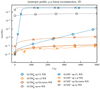 |
Fig. A.1. Same as Fig. 4, but as a 1D simulation. The adiabatic exponent is γ = 5/3. The solid lines represent the maximum Mach numbers on the grid. Time is given in units of the sound-crossing time tSC = 4.28 s. The curves have been slightly smoothed for better visibility. |
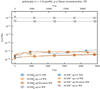 |
Fig. A.2. Same as Fig. 5, but as a 1D simulation. The adiabatic exponent is γ = 5/3. The solid lines represent the maximum Mach numbers on the grid. Time is given in units of Brunt–Väisälä time tBV = 20.1 s and sound-crossing time tSC = 4.13 s. The curves have been slightly smoothed for better visibility. |
Appendix B: Hot bubble
This appendix explores the amplitude dependence of the hot bubble test from Sect. 5.2.
 |
Fig. B.1. Same as Fig. 6, but showing the dependence of the solution on the initial amplitude (ΔA/A)t = 0 (left to right) on the 128 × 192 grid for the two best well-balancing methods (rows). The final time of the simulations is scaled with |

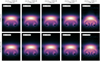 |
Fig. B.2. Mach-number distributions in the solutions shown in Fig. B.1. The color scheme ranges from 0 (black) to the maximum value (white) reached in the simulation box, which is also indicated at the top of the panels. |
Appendix C: Simple convective box setup
Table C.1 shows that the relative deviation from hydrostatic equilibrium in the convective box test from Sect. 5.3 scales with the square of the rms Mach number in the convection zone.
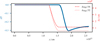 |
Fig. C.1. Varying vertical grid spacing as a function of the vertical coordinate y for the simulations shown in the center and right panels of the lower row in Fig. 13. The superadiabaticity is shown as a blue line, a negative value indicates a convectively stable stratification. The spacing changes smoothly to a finer resolution slightly before the transition to the stable zone starts. |
Relative deviation from hydrostatic equilibrium, rms Mach number, and ratio of the squared Mach number to the deviation at different heating rates.
Appendix D: Keplerian disk
Figure D.1 shows the time evolution of density in the Keplerian disk problem from Sect. 5.4.
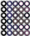 |
Fig. D.1. Snapshots of the density distribution during the evolution of the Keplerian disk. Shown are runs with deviation well-balancing and without well-balancing using explicit time stepping and resolutions of 20 × 70 cells as well as 100 × 350 grid cells. The bottom two rows show the same setup evolved with implicit time stepping at a resolution of 20 × 70 cells. To emphasize the deviation from the initial background density of 𝜚0 = 1 we show here 𝜚 − 1 and give the maximum and minimum of this quantity in an inset for each snapshot. |
All Tables
Relative deviation from hydrostatic equilibrium, rms Mach number, and ratio of the squared Mach number to the deviation at different heating rates.
All Figures
|
Fig. 1. Time evolution of the maximum Mach number in a 1D atmosphere with an isothermal temperature profile (Eq. (74)) and a linear gravitational potential (Eq. (73)). The colors indicate different well-balancing (WB) methods, the markers different flux functions. CL stands for Cargo–LeRoux. Time is given in units of the Brunt–Väisälä time tBV = 9.93 s (Eq. (18)) and sound-crossing time tSC = 3.10 s (Eq. (19)). The curves have been slightly smoothed for better visibility. |
| In the text | |
|
Fig. 2. Same as Fig. 1, but for a 2D atmosphere. The solid lines represent the maximum Mach numbers on the grid and the dotted lines the horizontal density fluctuations according to Eq. (75). The curves have been slightly smoothed for better visibility. |
| In the text | |
|
Fig. 3. Mach number (top panel) and horizontal density fluctuation Δ𝜚 (bottom panel) of the 2D isothermal simulation using the AUSM+-up flux and deviation well-balancing at time t = 1000 tBV. Gravity is directed in negative x-direction. |
| In the text | |
|
Fig. 4. Same as Fig. 2, but for an isentropic stratification. The solid lines represent the maximum Mach numbers on the grid and dotted lines the horizontal density fluctuations according to Eq. (75). Time is given in units of the sound-crossing time tSC = 4.28 s. The curves have been slightly smoothed for better visibility. |
| In the text | |
|
Fig. 5. Same as Fig. 2, but for a polytropic stratification with ν = 1.6. The adiabatic exponent is γ = 5/3. The solid lines represent the maximum Mach numbers on the grid and dotted lines the horizontal density fluctuations according to Eq. (75). Time is given in units of Brunt–Väisälä time tBV = 20.1 s and sound-crossing time tSC = 4.13 s. The curves have been slightly smoothed for better visibility. |
| In the text | |
|
Fig. 6. Time evolution (top to bottom) of the hot-bubble problem when solved using different well-balancing and reconstruction schemes (left to right) on a 128 × 192 grid. In all of the cases, entropy fluctuations ΔA/A are shown on the same color scale ranging from −10−3 (dark blue) through 0 (white) to 10−3 (dark red). The minimum and maximum values of ΔA/A in the whole simulation box are given in each panel’s inset. The amplitude of the initial entropy perturbation is (ΔA/A)t = 0 = 10−3. |
| In the text | |
|
Fig. 7. Same as Fig. 6, but showing the solutions’ resolution dependence (top to bottom) at t = 300 s. |
| In the text | |
|
Fig. 8. Dependence of the maximum Mach number Ma and minimum and maximum entropy fluctuations ΔA/A on the bubble’s initial amplitude (ΔA/A)t = 0. All measurements are taken when the bubble has evolved to a stage comparable to that shown in the bottom row of Fig. 6. Open and filled symbols correspond to runs with α-β and deviation well-balancing, respectively. The lines show that the Mach number scales according to Eq. (82) and the minimum and maximum entropy fluctuations scale in proportion to the bubble’s initial amplitude. |
| In the text | |
|
Fig. 9. Initial stratification of the convection setup. The red curve illustrates the position and shape of the energy injection which has nonzero values only at the bottom of the convection zone. Its actual amplitude is set for the different simulations individually. Dots denote the positions of cell centers on a grid with 144 vertical cells, the lowest resolution used in the SLH simulations presented in this section. |
| In the text | |
|
Fig. 10. Root mean square Mach number Marms as a function of the heating rate ė0. The dashed line represents the expected scaling according to Eq. (87). All values correspond to time averages over t ∈ [t(Nτ = 5), t(Nτ = 10)] (see text). The vertical error bars denote one standard deviation of the temporal average of Marms. |
| In the text | |
|
Fig. 11. Mach number of the flow for different values of the heating rate ė0 (left to right) and different well-balancing methods (top to bottom). The dashed black lines denote the boundaries of the convection zone at y = ytop, see Table 2 for an overview of simulation parameters. The insets displays the rms Mach number Marms within the convection zone for the snapshot shown. All snapshots are taken at t(Nτ = 7.5). |
| In the text | |
|
Fig. 12. Expected typical vertical wavelength (Eq. (90)) in grid cells of internal gravity waves as a function of Marms in two series of simulations with the deviation well-balancing method. Black crosses correspond to simulations at fixed resolution but increasing heating rate. Blue crosses correspond to simulations at a fixed heating rate but different resolution. The two encircled data points result from the same simulation but Marms has been determined at a different time. |
| In the text | |
|
Fig. 13. Mach number for a heating rate of ė0 = 104 and deviation well-balancing at different resolutions. The upper left box in each panel indicates the change in the vertical resolution relative to the resolution used for the Mach number scaling. The lower right box gives the total number of cells of the particular simulation. All snapshots are taken as soon as convection has fully developed. The dashed white line illustrates the profile of the Brunt–Väisälä frequency as a function of height with arbitrary units on the x-axis. |
| In the text | |
|
Fig. 14. Time evolution of the angle-averaged density profiles |
| In the text | |
|
Fig. 15. Left panel: geometry of the cubed-sphere grid. The number of cells has been reduced compared to grids used in the other two panels to ease the identification of individual cells and their shapes. Middle and right panel: shell convection in a setup comparable to that in Sect. 5.3 but with a shallower stratification and ideal gas EoS. Middle panel: color coded Mach number in a run without well-balancing. Numerical discretization errors quickly lead to spurious flows in the central region and the maximum Mach number reaches 3 × 10⁻². In the run with deviation well-balancing shown in the right panel the convective shell is clearly maintained. The maximum Mach number is 2 × 10⁻³. |
| In the text | |
|
Fig. A.1. Same as Fig. 4, but as a 1D simulation. The adiabatic exponent is γ = 5/3. The solid lines represent the maximum Mach numbers on the grid. Time is given in units of the sound-crossing time tSC = 4.28 s. The curves have been slightly smoothed for better visibility. |
| In the text | |
|
Fig. A.2. Same as Fig. 5, but as a 1D simulation. The adiabatic exponent is γ = 5/3. The solid lines represent the maximum Mach numbers on the grid. Time is given in units of Brunt–Väisälä time tBV = 20.1 s and sound-crossing time tSC = 4.13 s. The curves have been slightly smoothed for better visibility. |
| In the text | |
|
Fig. B.1. Same as Fig. 6, but showing the dependence of the solution on the initial amplitude (ΔA/A)t = 0 (left to right) on the 128 × 192 grid for the two best well-balancing methods (rows). The final time of the simulations is scaled with |
| In the text | |
|
Fig. B.2. Mach-number distributions in the solutions shown in Fig. B.1. The color scheme ranges from 0 (black) to the maximum value (white) reached in the simulation box, which is also indicated at the top of the panels. |
| In the text | |
|
Fig. C.1. Varying vertical grid spacing as a function of the vertical coordinate y for the simulations shown in the center and right panels of the lower row in Fig. 13. The superadiabaticity is shown as a blue line, a negative value indicates a convectively stable stratification. The spacing changes smoothly to a finer resolution slightly before the transition to the stable zone starts. |
| In the text | |
|
Fig. D.1. Snapshots of the density distribution during the evolution of the Keplerian disk. Shown are runs with deviation well-balancing and without well-balancing using explicit time stepping and resolutions of 20 × 70 cells as well as 100 × 350 grid cells. The bottom two rows show the same setup evolved with implicit time stepping at a resolution of 20 × 70 cells. To emphasize the deviation from the initial background density of 𝜚0 = 1 we show here 𝜚 − 1 and give the maximum and minimum of this quantity in an inset for each snapshot. |
| In the text | |
Current usage metrics show cumulative count of Article Views (full-text article views including HTML views, PDF and ePub downloads, according to the available data) and Abstracts Views on Vision4Press platform.
Data correspond to usage on the plateform after 2015. The current usage metrics is available 48-96 hours after online publication and is updated daily on week days.
Initial download of the metrics may take a while.