| Issue |
A&A
Volume 666, October 2022
|
|
|---|---|---|
| Article Number | A181 | |
| Number of page(s) | 15 | |
| Section | Cosmology (including clusters of galaxies) | |
| DOI | https://doi.org/10.1051/0004-6361/202243632 | |
| Published online | 24 October 2022 | |
Improving the accuracy of estimators for the two-point correlation function
Ludwig–Maximilians Universität München, Fakultät für Physik, Schellingstr. 4, 80799 München, Germany
e-mail: This email address is being protected from spambots. You need JavaScript enabled to view it.
Received:
24
March
2022
Accepted:
25
August
2022
Abstract
Aims. We show how to increase the accuracy of estimates of the two-point correlation function without sacrificing efficiency.
Methods. We quantify the error of the pair-counts and of the Landy & Szalay estimator by comparing them with exact reference values. The standard method, using random point sets, is compared to geometrically motivated estimators and estimators using quasi-Monte Carlo integration.
Results. In the standard method, the error scales proportionally to 1/√Nr, with Nr being the number of random points. In our improved methods, the error scales almost proportionally to 1/Nq, where Nq is the number of points from a low-discrepancy sequence. We study the run times of the new estimator in comparison to those of the standard estimator, keeping the same level of accuracy. For the considered case, we always see a speedup ranging from 50% up to a factor of several thousand. We also discuss how to apply these improved estimators to incompletely sampled galaxy catalogues.
Key words: methods: statistical / methods: data analysis / large-scale structure of Universe
© M. Kerscher 2022
 Open Access article, published by EDP Sciences, under the terms of the Creative Commons Attribution License (https://creativecommons.org/licenses/by/4.0), which permits unrestricted use, distribution, and reproduction in any medium, provided the original work is properly cited.
This article is published in open access under the Subscribe-to-Open model. This email address is being protected from spambots. You need JavaScript enabled to view it. to support open access publication.
1. Introduction
Statistical approaches are often used to characterise the large-scale structure of the galaxy distribution, wherein it is assumed that the distribution of galaxies is a realisation of a point process (see e.g. Neyman & Scott 1958; Peebles 1980). Observations give us the positions of galaxies in space. From this set of points, we estimate the moments of the point process, specifically the two-point correlation function ξ(r) or the two-point density
 (1)
(1)
the probability of finding two galaxies at x and y, where 𝜚 is the number density. In a homogeneous and isotropic point process, ξ(r) only depends on the separation r = |x − y|. To determine ξ(r) from a galaxy catalogue within a finite domain W ⊂ ℝ3, we use estimators. In cosmology, estimators based on random point sets are most commonly used. These rely on the data–data DD, data–random DR, and random–random RR pair-counts (see below for the definition).
The two-point correlation function of the galaxy distribution is often used to constrain models of structure and galaxy formation and to estimate parameters of cosmological models. In current and upcoming galaxy samples, the positions of millions and up to billions of galaxies will be observed (Dawson et al. 2013, BOSS; Ross et al. 2020, eBOSS; Abbott et al. 2022, DES; Aghamousa et al. 2016, DESI; Alarcon et al. 2021, PAUS; Ivezić et al. 2019, LSST; Amendola et al. 2018, Euclid). Fast and reliable methods for calculating the two-point correlation function are needed. These large samples allow us to reduce the statistical error from cosmic variance, but for the error budget of the two-point correlation function we also have to control the systematic errors. One systematic contribution is the error from random sets used in the pair-counts DR and RR. As an example, consider the baryon acoustic oscillations (BAOs) which lead to a peak in the two-point correlation function of galaxies at a scale of about 100 Mpc h−1 (Eisenstein et al. 2005; Bautista et al. 2021). This BAO peak has a height of approximately 0.01 above zero (compare Fig. 2 in Eisenstein et al. 2005). For a percent level accuracy, we need to calculate the two-point correlation function with an absolute accuracy of less than 10−4. Below, we show how to reduce the systematic error to this level of accuracy without sacrificing efficiency.
Several estimators for the two-point correlation function have been developed (Peebles & Hauser 1974; Hewett 1982; Davis & Peebles 1983; Rivolo 1986; Landy & Szalay 1993; Hamilton 1993). By comparing these estimators to a reference result from a cosmological simulation, Kerscher et al. (2000) found that the Landy & Szalay (1993) estimator is the preferred estimator with the smallest deviation from the reference and also that its bias is negligible compared to its variance.
We focus on methods for increasing the numerical accuracy of the pair-counts as used in these estimators. The random point set, shared in the pair-counts RR and DR is used to correct for boundary (finite-size) and inhomogeneous sampling effects. As we outline below, RR and DR are Monte Carlo volume integration schemes. As expected from standard Monte Carlo integration, the error of these pair-counts RR and DR scales at least as  , where Nr is the number of random points used (see Sect. 3 for a more differentiated view). This slow convergence rate makes increasing the accuracy costly, and sometimes unfeasible. To improve the accuracy of the pair-counts without sacrificing efficiency, we follow two directions:
-
The pair-counts can be expressed as averages of specific volume fractions. We use this to propose special adapted volume integration schemes which, in turn, can be calculated more efficiently than the standard approach.
-
We replace the standard Monte Carlo scheme with a quasi-Monte Carlo integration, which leads to an improved scaling of the error that is almost proportional to 1/Nq, where Nq is the number of points from a low-discrepancy sequence.
We compare the standard and the new methods to exactly known reference values. This allows us to empirically validate the asymptotic scaling of the errors.
A variety of approaches have been suggested to improve the speed and accuracy of estimators for the two-point correlation function. Keihänen et al. (2019) show that at fixed computational cost, a split random catalogue improves the accuracy of estimators for the two-point correlation function. For galaxy catalogues, Demina et al. (2018) achieve a speedup by factorising the calculations in radial (redshift) and angular coordinates (see also Breton & de la Torre 2021). Perhaps closest to our work are the investigations by Dávila-Kurbán et al. (2021). These authors use glass-like point sets instead of the random catalogues, where we use low-discrepancy sequences. As reference values in our comparisons, we use the exact results from Baddeley et al. (1993) and Kerscher (1999) for a rectangular box as summarised in Appendix B (for periodic boxes see Appendix A.1). He (2021) also discusses some approximations for these exact results.
Other approaches focus on the computational problem of calculating the pair-counts. Tree-based methods can be significantly faster than a direct implementation of the pair-counts, specifically for small radii (Moore et al. 2001, see also Appendix C). The double loop in the pair-count calculations can be parallelised. Alonso (2012) showed how to obtain a speedup by a factor of 100 over the direct implementation by using multi-threading on multi-core CPUs or utilising many cores in GPUs. It is well known from matrix computations that the memory layout of the data can have dramatic consequences for the run time of algorithms (see e.g. Anderson et al. 1999). Also, for the pair-counts, a clever layout of the coordinates in the memory can lead to a significant speedup (Donoso 2019). A similar approach can be combined with multi-threading and vectorisation resulting in a blazingly fast code (Sinha & Garrison 2020). Our conceptual improvements can be combined with these computational speedups.
In Sect. 2 we give the definition of the pair-counts and discuss the geometry of the expected pair-counts. In Appendix A we give the details of the derivations and in Appendix B we summarize some results for simple sample geometries. Together with Sect. 2, this enables us to calculate exact reference values for the pair-counts. At the end of Sect. 2, we give a short introduction to the quasi-Monte Carlo method, as used in our improved estimators. In Sects. 3 and 4, we compare the standard and improved versions of the pair-counts with the exactly known reference values. We discuss the scaling of the error with the number of points. We put this together in Sect. 5 and show how an improved version of the Landy & Szalay (1993) estimator can be constructed. Again we discuss the scaling of the error with the number of points. In Sects. 5.1 and 5.2, we compare the run times of the new estimator with those of the standard Landy & Szalay (1993) estimator in some typical situations. In Sect. 6, we discuss how these improvements have to be adapted to estimate the two-point correlation function from an inhomogeneous sampled galaxy distribution. We summarise in Sect. 7 and give some recommendations. In Appendix C, we discuss details of the implementation, the run times, and give a link to the code.
2. Pair-counts, geometry, and quasi-Monte Carlo
The set of the N data points (e.g. galaxies) is  with all points xi ∈ W inside the observation window W ⊂ ℝ3, that is, inside the unmasked area. The number density is estimated with
  , where |W| is the volume of W. We then define
 (2)
(2)
the normalised number of data–data pairs with a distance of r = |xi − xj| in the interval [r, r + δ]. We use a rectangular kernel
![Mathematical equation: $$ \begin{aligned} k_r^{\delta }(s) = \tfrac{1}{{\delta }}{\mathbb{1} }_{[r,r+{\delta }]}(s), \end{aligned} $$](/articles/aa/full_html/2022/10/aa43632-22/aa43632-22-eq7.gif) (3)
(3)
with the indicator function of the set A defined as
 (4)
(4)
Also, other kernels with  are possible (e.g. triangular, truncated Gaussian, or Epanechnikov). We consider Nr randomly distributed points
  , all inside the sample geometry yj ∈ W. The normalised number of data-random pairs with a distance in [r, r + δ] is denoted by
 (5)
(5)
Similarly,
 (6)
(6)
is the normalised number of random–random pairs. The Landy & Szalay (1993) estimator is defined as
 (7)
(7)
Also, the estimators provided by Peebles & Hauser (1974), Hewett (1982), Davis & Peebles (1983), and Hamilton (1993) can be defined in terms of the pair-counts and our results apply accordingly.
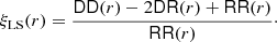
2.1. Geometry of pair-counts
The expectation of the pair-counts DR and RR can be expressed in terms of geometric quantities depending on the sample window W and on the point set (for DR, Kerscher 1999). We first consider the set-covariance
 (8)
(8)
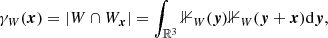
where Wx is the shifted window W, that is, the set of all points from W shifted by the vector x. |W ∩ Wx| is the volume of the set W ∩ Wx. The isotropised set-covariance  can be calculated from γW(x):
 (9)
(9)
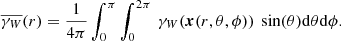
Here x(r, θ, ϕ) = (rcos(ϕ)sin(θ),rsin(ϕ)sin(θ),rcos(θ)). For a large number of random points Nr one obtains (see Appendix A):
 (10)
(10)
where ℛℛ(r) is the expectation value of the pair-count RR(r) illustrating its geometric nature.
Ripley (1988) used a local area weight in an estimator for his K-function (the normalised integrated two-point density) and Rivolo (1986) considered a similar weight in his estimator for the two-point correlation function. This weight is inversely proportional to the fraction of the surface area of a sphere Br(y) with radius r centred on the point y inside W:
 (11)
(11)
For a large number of random points Nr, one obtains (see Appendix A):
 (12)
(12)
As before, 𝒟ℛ(r) is the expectation value of the pair-count DR(r) illustrating its geometric nature. However, now both DR(r) and 𝒟ℛ(r) are depending on the points  under consideration.
In Appendix B, we give expressions for  and area(∂Br(y)∩W) if W is a rectangular box or a sphere. From these expressions, we calculate the reference values 𝒟ℛ and ℛℛ. This allows us to compare different integration schemes for the pair-counts DR and RR and we can investigate the scaling of the accuracy with the number of points used in these methods.
2.2. Quasi-Monte Carlo
In our improved methods for estimating the pair-counts, we use quasi-Monte Carlo integration. In a standard Monte Carlo integration scheme, one uses Nr random points {y1, …, yNr} to estimate the integral ∫[0, 1]df(x)dx by  . The accuracy can be estimated using the Chebyshev inequality, which tells us that the probability of an error exceeding a given threshold decreases with
  . In other words, the standard error of a Monte Carlo integration scales as
  .
.
With quasi-Monte Carlo methods, we use  to numerically integrate ∫[0, 1]df(x)dx (see e.g. Niederreiter 1992). This estimate of the integral almost looks identical to the Monte Carlo integration above. However, for a quasi-Monte Carlo integration, the points in Q = {q1, …, qNq} are not random. It is essential for the application of quasi-Monte Carlo integration that for a given point set Q the error bound
![Mathematical equation: $$ \begin{aligned} \left| \int _{[0,1]^d} f(\boldsymbol{x})\mathrm{d} {\boldsymbol{x}} - \frac{1}{{{N_{\rm q}}}} \sum _{i=1}^{{N_{\rm q}}}f({\boldsymbol{q}}_i)\right| \le V(f)\, D(Q) \end{aligned} $$](/articles/aa/full_html/2022/10/aa43632-22/aa43632-22-eq26.gif) (13)
(13)
factorises into a measure of variation V(f) depending only on properties of f, and a measure of discrepancy D(Q) depending only on the properties of the point set Q. If we consider functions of bounded variation, Eq. (13) is referred to as the Koksama-Hlawka bound and the measure of discrepancy is the star discrepancy (see e.g. L’Ecuyer & Lemieux 2002). To control the error bound (Eq. (13)), we have to control D(Q) (we note that V(f) does not depend on the point set Q). Low-discrepancy sequences, such as the Halton sequence, have been constructed with that in mind. For such sequences, Halton (1960) showed that
 (14)
(14)
For small dimensions, d, this compares favourably to a Monte Carlo integration where the standard error only scales as  . Halton sequences can be used to estimate integrals over indicator functions, which in turn define volumes like the set covariance. As indicator functions have bounded total variation, Eq. (13) applies.
Upper bounds like Eq. (13) are worst-case bounds. Owen & Rudolf (2021) derive an analogue to a strong law of large numbers for randomised low-discrepancy sequences. This further justifies the procedure for scrambling the Halton sequence developed by Owen (2017), where the scaling from Eq. (14) in Eq. (13) still gives an upper bound, but on average smaller errors are expected. We use these randomised Halton sequences in our calculations (see Appendix C).
3. RR
First we investigate how the accuracy of the standard RR, as given in Eq. (6), scales with the number of random points used. The numerical implementation of the pair-counts is discussed in Appendix C. The expectation value ℛℛ of RR can be expressed in terms of the isotropised set-covariance; see Eq. (10). Using the Eqs. (B.1) and (B.3) for the isotropised set covariance, we calculate ℛℛ(r) as a reference value for rectangular boxes W.
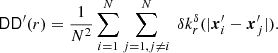
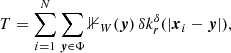
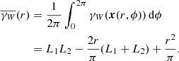
Figure 1 shows the scaling of the relative error εRR = |ℛℛ(r)−RR(r)|/ℛℛ(r) with the number of random points used. The error εRR is the mean value calculated from 100 samples of the random point sets. Only for the largest Nr do we use 10 samples. This also applies to the errors calculated in the following sections. We show the results for a rectangular cuboid W = [0, 1]3 and for a thin rectangular box W = [0, 1]×[0, 0.1]2. With the thin box, we investigate how the error is affected in a sample W where the boundary effects are more dominant. Landy & Szalay (1993, their Eq. (21)) show that the relative error of RR is of the form  , with A and B depending on the window W and the bin width. As expected, we see in Fig. 1 that the error scales as
  for large Nr. For small Nr and small radii, the contribution proportional to 1/Nr appears. This additional contribution can be seen in the voluminous sample but not in the thin box. Simply using a three-dimensional low-discrepancy sequence instead of the random points in Eq. (6) is not feasible, as we see below.
 |
Fig. 1. Relative error εRR against the number of random points Nr used in the standard procedure for calculating RR(r) in rectangular windows W. The black dotted lines are proportional to 1/Nr and |

From Eqs. (A.4) and (A.5) we get
 (15)
(15)
This allows a more flexible approach. Consider two (random) point sets  and
and  , with the points yi ∈ W, zj ∈ W all inside the sample geometry. We then define
 (16)
(16)
which is also an estimate of ℛℛ(r). If the points in P1 and P2 are drawn from a Poisson process, the estimate from Eq. (16) is almost the same as the estimate from Eq. (6), because points in a Poisson process are independent. See also Dávila-Kurbán et al. (2021), who observe that one cannot use P1 ≡ P2 for RR2x3d when they construct an estimator for the two-point correlation function using ‘glass like’ point sets. The representation of ℛℛ in Eq. (15) as a six-dimensional integral suggests a six-dimensional (quasi-)Monte Carlo approach. Consequently, we use six-dimensional random points or a six-dimensional randomised Halton sequence  , which we split as qi = (yi, zi) into two three-dimensional sequences. We scale the points in the sequences
  and
and  such that each yi ∈ W and zj ∈ W are uniformly distributed inside the sample geometry.
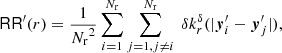
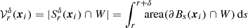
Figure 2 compares the scaling of the relative error εRR, 2x3d = |ℛℛ(r)−RR2x3d(r)|/ℛℛ(r) with the number of (quasi-)random points. For random points, we see the expected scaling  of the error. Using the quasi-Monte Carlo approach, we see that the error scales proportionally to 1/N, which is even faster than the theoretical expectation according to Eq. (14). Using a low-discrepancy sequence, we gain more than two orders of magnitude in accuracy compared to the random point sets.
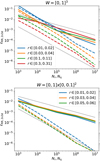 |
Fig. 2. Relative error εRR, 2x3d calculated for rectangular windows W with a pure Monte Carlo integration (solid lines) and with a randomised Halton sequence (dashed lines). The black dotted lines are proportional to |

4. DR
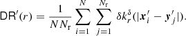
In Sect. 2.1 we show that the expectation of DR(r) is 𝒟ℛ(r) and that it can be calculated from the area fraction area(∂Br(xi)∩W). For a rectangular box, Baddeley et al. (1993) gave explicit expressions for area(∂Br(xi)∩W) (see Appendix B.1). We use these expressions to calculate 𝒟ℛ(r) according to Eqs. (A.9) and (A.10). In the numerical integration of Eq. (A.9), we make sure to achieve a relative error of at least 10−10 for our reference value 𝒟ℛ(r). Both DR(r) and 𝒟ℛ(r) depend on the point set under consideration. We need a realistic data set D =  to calculate both the theoretical reference 𝒟ℛ(r) and the different estimates for DR(r). For this purpose, we use a sample of simulated galaxy clusters1 from the Magneticum simulation (Hirschmann et al. 2014; Ragagnin et al. 2017). The side length of the simulation box is 325 Mpc h−1 and we use the real space positions of the 10 429 simulated clusters. We rescale the coordinates by the side-length of the box such that all points are inside W = [0, 1]3. In the smaller window W = [0, 1]×[0, 0.1]2 only 86 clusters are left.
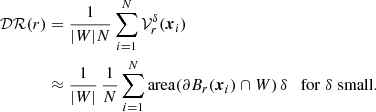
Now we are set to determine the scaling of the relative error εDR = |𝒟ℛ(r)−DR(r)|/𝒟ℛ(r) with the number of (quasi-)random points used. Figure 3 compares the standard approach with ordinary random numbers in DR(r) to a pair-count determined using a low-discrepancy sequence instead of the random points. Using a randomised Halton sequence, we only observe a minor gain for small N, but for large N the error is reduced by an order of magnitude. In the small window, W = [0, 1]×[0, 0.1]2, this is more pronounced. The scaling follows the expected behaviour from Eq. (14).
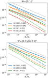 |
Fig. 3. Relative error εDR calculated for rectangular windows W with a standard Monte Carlo integration (solid lines) and with a quasi-Monte Carlo scheme using a randomised Halton sequence (dashed lines). The black dotted lines are proportional to |

We can do better if we consider the geometry of DR(r). From Eqs. (A.9) and (A.10) we know that the expectation value of DR(r) is  , where
 (17)
(17)
is the volume of the spherical shell with a radial range in [r, r + δ] around xi inside the sample geometry W. As already suggested by Rivolo (1986), this directly leads to a Monte Carlo scheme. With Nsh points  (quasi-)randomly distributed in the shell
  around xi we define a (quasi-)Monte Carlo estimate of
  :
:
 (18)
(18)
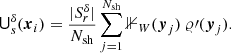
with the volume  of the shell. We then get
  for a large number Nsh of (quasi-)random points. Consequently we compare
 (19)
(19)
with 𝒟ℛ(r). This is not a pair-count, but we still have a double sum over N data points and now Nsh points in the shell.
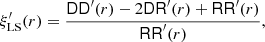
Figure 4 shows εDR, shell = |𝒟ℛ(r)−DRshell(r)|/𝒟ℛ(r). A comparison with DR in Fig. 3 shows that using DRshell leads to a reduction of the error by almost two orders of magnitude even for ordinary random points. Again this can be improved by using low-discrepancy sequences; doing so allows us to additionally gain at least another order of magnitude.
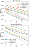 |
Fig. 4. Relative error εDR, shell calculated for rectangular windows W with a pure Monte Carlo integration (solid lines) and with a randomised Halton sequence (dashed lines). The black dotted lines are proportional to |

5. Estimating ξ
Now we join the improved pair-count estimates together and compare results from the standard Landy & Szalay (1993) estimator to our new estimator for the pair correlation function. We use the simulated galaxy clusters from the Magneticum simulation to illustrate the behaviour of the different estimators (Hirschmann et al. 2014; Ragagnin et al. 2017, compare also Sect. 4). The 10 429 clusters are in a box with side-length 325 Mpc h−1 and we use their real space positions. The standard Landy & Szalay (1993) estimator was defined in Eq. (7):

First we use the same Nr random points to calculate RR and DR (see Eqs. (5) and (6)). As an exact reference we have
 (20)
(20)
with the ℛℛ and 𝒟ℛ given in Eqs. (10), (12), using the results from Appendix B.1 for a rectangular box. In Sects. 3 and 4 we discuss alternative possibilities to calculate the pair-counts DR and RR. We focus on the following combination:
 (21)
(21)
which resembles the Landy & Szalay (1993) estimator, but now with improved pair-count estimates. We use a low-discrepancy sequence with Nshell 3D points to calculate DRshell (see Eq. (19)), and another 6D low-discrepancy sequence with N2x3d points to calculate RR2x3d (see Eq. (16)).
As an illustrative example we compare these estimates in Fig. 5 using an insufficient number of points. As expected, we observe that a standard Landy & Szalay (1993) estimator with only 104 random points shows deviations from the exact result, but with 105 random points the LS-estimator starts to follow the exact result. Visually, one can see that the estimator using the low-discrepancy sequences achieves a higher accuracy already with N2x3d = 104 = Nsh points.
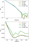 |
Fig. 5. Two-point correlation function calculated for a simulated galaxy cluster sample. The exact Ξ is compared to standard ξLS with Nr = 104 and Nr = 105 random points, and to the new |

To make this quantitative and to disentangle the influence that these different methods for calculating DR and RR have, we consider the ‘half exact’ estimates for ξ(r):
 (22)
(22)
where we use the exact reference values ℛℛ and 𝒟ℛ in turn. We also calculate Ξℛℛ and Ξ𝒟ℛ using DRshell and RR2x3d instead of DR and RR. For the comparison, we consider the absolute error Δ1(r) = |Ξ(r)−Ξ𝒟ℛ(r)| and Δ2(r) = |Ξ(r)−Ξℛℛ(r)|. In Fig. 6 we see that the scaling investigated in Sect. 3 directly transfers to the scaling of the error in the estimated ξ. For a fixed number of (quasi-)random points, RR2x3d is more accurate. The gain in accuracy is considerable for intermediate and large radii. For small radii and for a smaller number of (quasi-)random points, the accuracy gain of RR2x3d is reduced to a factor of two. With the standard DR, the error Δ1 scales as  (see Fig. 7). Already using a low-discrepancy sequence instead of random points in DR leads to a reduction in the error and the scaling starts to follow 1/Nq. Compared to DR, the DRshell gives a significantly smaller error, again showing a scaling proportional to 1/Nsh. This reduced error comes at a price: the run time of DRshell is greater than the run time of DR for the same number of (quasi-)random points (see Appendix C).
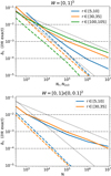 |
Fig. 6. Absolute error Δ1 is shown for the standard RR (solid lines) and for RR2x3d (dashed lines) pair-counts. The black dotted lines are proportional to |

5.1. Run time
Ultimately, we are not interested in the scaling of the error with the number of (quasi-)random points. We want to obtain reliable results fast. The speed of the calculation depends on the hardware platform, the algorithms, details of the implementation, and further effects (see Appendix C). Nevertheless, we prepared some examples and investigate what one can expect as a speedup when using the new estimator. In a given window, and for a given radius interval, we look at Figs. 6 and 7 to read off how many (quasi-)random points we approximately need to achieve a targeted absolute error. In most applications of the standard estimator ξLS, the same random point set is used with RR and DR. However, there is some room for optimisation. As we tune RR2x3d and DRshell in the new estimator separately, we also choose different sizes of the random samples in RR and DR to optimise the overall run time. With some provisional runs, we check that we achieve the targeted accuracy Δ within 10%; sometimes we had to adjust the numbers. Table 1 lists the final parameters we use. For case III, we use Nr = 107 and achieve a Δ ≈ 5 × 10⁻⁴ for the standard estimator, and therefore the run times for case III may serve only as a lower bound.
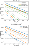 |
Fig. 7. Absolute error Δ2 is shown for the standard DR (solid lines), the DR using a low-discrepancy sequence (dotted lines), and for DRshell also using a low-discrepancy sequence (dashed lines). The black dotted lines are proportional to |

Parameters and results of the run-time comparison.
The comparison of the run times was conducted on a small workstation (for details see Appendix C). We estimate the run times from 100 runs, for the longer running calculations we use 20 runs (in case III 5 runs). As the targeted accuracy is matched at the 10% level and this comparison did not run on an isolated machine, we can only give one digit for the run times. See Appendix C for further comments on the run time calculations.
The run times of the pair-counts are shown in Table 1 for different windows, radius ranges, and for different targeted accuracies. From Appendix C, we know that for a fixed number of (quasi-)random points, the standard pair-counts RR and DR are always faster than the corresponding RR2x3d and DRshell. However, we choose the number of (quasi-)random points by requiring a given accuracy. In that case, we need fewer points for the new pair-counts, which in turn lowers their run times. Now we compare RR and RR2x3d as well as DR and DRshell at fixed accuracy, and find that the run times of the new pair-counts are smaller in all the considered cases. We also see from Table 1 that the relative significance of the RR, RR2x3d and DR, DRshell parts depends on the considered case. For a targeted high accuracy (small Δ), the run times are dominated by the RR and RR2x3d part, respectively. For small radii and for lower accuracy, the DR and DRshell parts dominate the run time. The geometry of the window further differentiates this picture. In Table 2, we sum up the parts and show the run times of ξLS and the new  . In all the cases considered, we see a reduction in the run time using the new estimator. For high accuracy and for large and intermediate radii, the effect is considerable. Using the new estimator we expect a reduction in run time by a factor of between several hundred and almost 104. For small radii and for less demanding accuracy goals, our method performs at least as well as the standard estimator and we may expect a reduction by up to an order of magnitude. The timing results for DD, RR, RR2x3d and DR are independent of the number of radius intervals, because we can sort the counts into the radius bins. However, we need to repeat the DRshell calculation for each radius bin.

5.2. A dense sample
Case VI from Table 1 shows that for small radii and lower accuracy goals, the run time is dominated by the DR or the DRshell calculations. However, DR and DRshell show very different run times depending on the number of data points (see Appendix C). Hence per se it is not clear which of the methods is preferable in dense samples for small radii and relaxed accuracy goals. We cannot check this with the cluster sample with N = 10429 data points only. Therefore, we use a sample of 1.36 million simulated galaxies2 from the Magneticum simulation (Hirschmann et al. 2014; Ragagnin et al. 2017) in the box with side-length 325 Mpc h−1. In Fig. 8, we see that the errors of RR and RR2x3d both scale proportionally to 1/Nr (see the discussion in Sect. 3). For a fixed number of (quasi-)random points, the RR2x3d is about twice as accurate as the RR for r ∈ [2, 3] Mpc h−1 in this dense sample. However, the accuracies of DR and DRshell differ drastically. Using the same number of points, accuracy is increased when using DRshell instead of DR by at least a factor of 103. We can understand this by looking at Eq. (19). In calculating DRshell, we average the shell volume inside the window over all the points. With so many points in this dense sample, only a rough estimate of the shell volume for each individual point or galaxy is necessary to obtain a DRshell of sufficient accuracy.
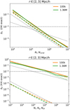 |
Fig. 8. Errors for estimates of the correlation function at r ∈ [2, 3] Mpc h−1 from 1.36 million galaxies and a subsample of 100 k galaxies in a box with side-length 325 Mpc h−1. Upper plot: absolute error Δ1 shown for the standard RR (solid lines) and for RR2x3d (dashed lines) pair-counts. Lower plot: absolute error Δ2 is shown for the standard DR (solid lines), the DR using a low-discrepancy sequence (dotted lines), and for DRshell also using a low-discrepancy sequence (dashed lines). The black dotted lines are proportional to |

We proceed as in Sect. 5.1, choose a targeted accuracy Δ = 10−2, and determine the required number of points Nr, N2x3d, and Nsh in the pair-counts as summarised in Table 3. Extrapolating from Fig. 8, we could have guessed that the number Nsh of points, as used in DRshell, is less than one. Instead of subsampling the galaxies, we simply use Nsh = 1, and therefore we are overestimating the required run time TDR, shell. It is also interesting to observe that in case XI we only need Nr ≪ N random points for the pair-counts in the standard estimators to achieve the targeted accuracy.
From Table 3 we see that for the subsampled galaxy distribution (case X, 100 k points), the pair-counts RR and DR have a comparable contribution to the run time for the standard estimator, whereas for the new estimator, the RR2x3d still provides the major contribution to the run time. For the full galaxy sample with 1.36 million galaxies, the dominant contribution is from DD followed by DR for the standard estimator. For the new estimator, both RR2x3d and DRshell contribute similarly to the run time. In both cases, the new estimator is still faster than the standard estimator, although only marginally in the full sample XI. These timing results should be considered with some reservation. As illustrated in Appendix C, a tree-based method can speedup the DD, RR, DR, and RR2x3d for small radii significantly. For DRshell, such a method for increasing the speed is currently unknown. This certainly affects the relative contribution of DR versus DRshell and depending on the situation, DR using a tree-based method can be faster than DRshell.
6. Incomplete sampling
The random points in RR and DR are not only used to correct for finite-size effects but also to correct for incomplete sampling. Here, we follow the ideas presented in Baddeley et al. (2000) and Shaw et al. (2021) and adapt them for the pair-counts. In this way, we can still use the new improved estimators and also correct for incomplete sampling.
Typically the galaxy distribution is observed incompletely. For example, unobserved regions around bright stars are masked. This leads to holes in the observational window W and can be dealt with using the methods already described. However, a partial sampling of the galaxy distribution in crowded fields leaves us with an inhomogeneous selection of the galaxy sample. Also, in magnitude-limited samples, we have a systematic selection of the galaxies, depending on the distance from us. We model this by p(x)∈(0, 1], the probability of including or observing a galaxy at position x. We assume that this p(x) is statistically independent of any other point in the galaxy distribution. For example, in a crowded field, only a fraction of the galaxies are randomly targeted for spectroscopic follow up. For a galaxy in this field, we have a p(x) equal to the fraction of targeted galaxies in the field. In a magnitude-limited sample, we observe all galaxies down to a limiting brightness llim. The luminosity of a galaxy L(d(x),l) at position x can be determined from the brightness l > llim and its luminosity distance d(x) from our galaxy (we neglect absorption for simplicity). Therefore, at a distance of d we only include galaxies with luminosity L > L(d, llim) in our catalogue. Now consider F(L), the distribution function of the absolute luminosities of all the galaxies (i.e. the normalised cumulative luminosity function). The fraction of galaxies included at a distance d(x) is then p(x) = 1 − F(L(d(x),llim)). We therefore need a good model for the luminosity function. The exclusion of a galaxy due to fibre collision cannot be modelled with the independent thinning (see below), and the following approach may only serve as an approximation. Further selection and sampling effects are discussed in Ross et al. (2012).
To investigate the effects of incomplete sampling, we assume an unobserved homogeneous and isotropic galaxy distribution G with number density 𝜚G and two-point correlation function ξG(r). Our goal is to estimate this ξG(r). The inhomogeneous sampling, described by p(x), leads to an observed inhomogeneous galaxy catalogue and is modelled in the following way:
 (23)
(23)
where ui are independent random variables that are specifically independent of the points and uniformly distributed on [0, 1]. This closely follows the construction of an inhomogeneous Markov point process by independent thinning as discussed by Baddeley et al. (2000). The observed inhomogeneous point set  is considered a realisation of D′. With the number density 𝜚G of the homogeneous galaxy distribution, the inhomogeneous number density of this point process is 𝜚′(x) = p(x) 𝜚G. The two-point density, the probability of observing a point at x and y, is
 (24)
(24)
This is well defined for a certain class of point process as defined in Baddeley et al. (2000). As the thinning is assumed to be independent from the points, we have
for the two-point correlation function.
In full analogy to Sect. 2, we define the ‘inhomogeneous’ pair-counts DD′. The points  are the incompletely sampled galaxies with positions
  inside the observation window W. Then
 (25)
(25)
To account for the effect of incomplete sampling, one often applies the thinning as described in Eq. (23) to the random points as well. In this way, our random point set  is a realisation of an inhomogeneous Poisson process with number density
  . The pair-counts involving these inhomogeneous random points are
 (26)
(26)
and
 (27)
(27)
Appendix A.2 shows that the Peebles & Hauser (1974) estimator using DD′ and RR′ is ‘ratio unbiased’. For the Landy & Szalay (1993) estimator, we combine the pair-counts DD′, DR′, and RR′ with
 (28)
(28)
in full analogy to Eq. (7). Now we show how we can calculate these inhomogeneous pair-counts using our new approach based on quasi-Monte Carlo methods. For this we make a detour and consider the expectation value of RR′ and then DR′.
For a large number of random points Nr from an inhomogeneous Poisson process, we obtain (see Appendix A.2):
 (29)
(29)
where  is given in Eq. (A.16), and ℛℛ′(r) is the expectation value of the pair-count RR′(r). There is no longer a direct correspondence with geometric objects like the set-covariance, however we can write ℛℛ′ as the following integral (compare to Eq. (15)):
 (30)
(30)
This suggests a (quasi-)Monte Carlo approach similar to Eq. (16). We use homogeneously sampled point sets P1, P2 as described in Sect. 3. Then
 (31)
(31)
is an estimate of ℛℛ′(r) (we reiterate that the number density of the inhomogeneous Poisson process is  ). As described in Sect. 3, the point sets P1, P2 can be generated from a six-dimensional random sequence or six-dimensional low-discrepancy sequence.
In Eq. (27) we use a thinned random point set to calculate DR′. Similarly, we could use a thinned low-discrepancy sequence in Eq. (27), but in Sect. 4 we see that this first approach is only mildly successful. We therefore follow the second approach by considering Eq. (A.18) and find
 (32)
(32)
where  is given in Eq. (A.19). Similar to Eq. (18), we use Nsh points
  (quasi-)randomly distributed in the shell
  around xi to estimate
  by
by
 (33)
(33)
This results in a new estimate for 𝒟ℛ′(r):
 (34)
(34)
Similar to Eq. (21) we can use DD′,  , and
, and  to construct a Landy & Szalay (1993) – type estimator
  for inhomogeneously sampled galaxy catalogues.
Shaw et al. (2021) discuss how to estimate the ξ′(r) and a non-parametric model for 𝜚′(x) directly from the data. In a typical application to galaxy catalogues, we often have a good model for 𝜚′(x) (or equivalently for p(x)). Parameters of this model are fixed by the sampling strategy, and some are determined from the galaxy distribution (e.g. from an estimate of the luminosity function).
7. Summary and outlook
First, we focussed on the scaling of the error in estimates of the pair-counts RR and DR with the number of (quasi-)random points. For the standard approach, with ordinary random numbers, we confirm the expected slow shrinking of the error proportional to  . A reformulation of the pair-counts makes a quasi-Monte Carlo integration possible. There we find that the error shrinks almost proportionally to 1/Nq, where Nq is the number of points from a low-discrepancy sequence. This scaling of the error not only holds for bulky samples but is even more pronounced in a thin sample with prevalent boundary effects. We are therefore confident that our improved methods are also applicable in more complicated sample geometries. We combine these improved pair-counts into a new Landy & Szalay (1993) – type estimator and compare with the standard one. The new estimator inherits the favourable scaling proportional to 1/Nq.
We can turn this observation around. For a fixed maximum error, we read off how many points are necessary to stay below this error with both the new and the standard estimator. We then compare the run times of the estimators. Depending on the accuracy goal, the radius range considered, and the density of the data, we observe a speedup by 50%, and up to a factor of almost 104 for our improved estimator. More specifically, using RR2x3d instead of the standard RR will increases the efficiency (accuracy vs. run time) of the estimator in any considered case. As tree-based methods are equally applicable to RR and RR2x3d, we recommend using RR2x3d for any use case. Also, in all the cases we considered, the DRshell is faster than the standard DR at fixed accuracy. However, an unreserved recommendation is not possible. For the DR calculations, a tree based method could be employed to speed up the calculations (we did not use one in our calculations). Currently, no comparable method for a speedup is known for DRshell. Therefore, in some situations for fixed accuracy, a tree-based method could lead to smaller run times in the DR calculations than in the DRshell calculations. We expect this to be relevant for voluminous samples, small radii, and lower accuracy goals. A combination of DD, DR, RR2x3d similar to Eq. (21) might therefore be useful. For large radii, we recommend DRshell.
The random point sets are not only used for boundary corrections but to correct for incomplete sampling as well. Typically, the selection and sampling effects, as present in the galaxy distribution, are modelled onto the random point set used in the pair-counts. We discuss how to adapt this for the new improved estimator; we are using the probability of observing the galaxies as a weight in the calculation of the pair-counts. However, this is only a first step. Using weighting schemes, one could envision the construction of a minimum variance estimate for inhomogeneous sampled galaxies, similarly to Saunders et al. (1992), Feldman et al. (1994), and Colombi et al. (1998), but now for the improved estimators using low-discrepancy sequences.
Our use of the randomised Halton sequence is similar to the use of glass-like point sets by Dávila-Kurbán et al. (2021). Generating glass-like point sets can be computationally challenging. In contrast, a randomised Halton sequence is generated easily (see Appendix C). Halton sequences are probably the simplest choice, but other low-discrepancy sequences could be used as well (L’Ecuyer & Lemieux 2002). Interesting alternatives could be the so-called blue noise random sets, which are used in computer graphics for efficiently sampling from surfaces (see e.g. Heck et al. 2013). The computational improvements like tree-based methods or optimised memory layout are complimentary to our approach and can be used similarly for the pair-counts with low-discrepancy sequences. This should lead to a further speedup.
Specifically we use the simulated galaxy clusters from the snapshot Box2/hr, snap_136, z = 0.066340191 downloaded from http://www.magneticum.org/data.html#FULL_CATALOUGES
We use the simulated galaxies from the snapshot Box2/hr, snap_136, z = 0.066340191 downloaded from http://www.magneticum.org/data.html#FULL_CATALOUGES
You find a basic version of the code at https://homepages.physik.uni-muenchen.de/~Martin.Kerscher/software/accuratexi/.
Acknowledgments
Many thanks to Adrian Baddeley for sharing code and the comments on the expressions for the area fraction. It is a pleasure to thank Klaus Dolag and Antonio Ragagnin for providing public access to the simulated galaxies and galaxy clusters from the Magneticum simulation. Also many thanks to the referee for his/her helpful comments and especially for the suggestion to include a more detailed discussion of the run times.
References
- Abbott, T. M. C., Aguena, M., Alarcon, A., et al. 2022, Phys. Rev. D, 105, 023520 [CrossRef] [Google Scholar]
- Aghamousa, A., Aguilar, J., Ahlen, S., et al. 2016, ArXiv e-prints [arXiv:1611.00036] [Google Scholar]
- Alarcon, A., Gaztanaga, E., Eriksen, M., et al. 2021, MNRAS, 501, 6103 [NASA ADS] [CrossRef] [Google Scholar]
- Alonso, D. 2012, ArXiv e-prints [arXiv:1210.1833] [Google Scholar]
- Amendola, L., Appleby, S., Avgoustidis, A., et al. 2018, Liv. Rev. Relativ., 21, 2 [NASA ADS] [CrossRef] [Google Scholar]
- Anderson, E., Bai, Z., Bschof, C., et al. 1999, LAPACK Users Guide, 3rd edn. (Philadelphia: SIAM) [CrossRef] [Google Scholar]
- Baddeley, A., & Turner, R. 2005, J. Stat. Softw., 12, 1 [CrossRef] [Google Scholar]
- Baddeley, A. J., Moyeed, R. A., Howard, C. V., & Boyde, A. 1993, Appl. Stat., 42, 641 [CrossRef] [Google Scholar]
- Baddeley, A. J., Møller, J., & Waagepetersen, R. 2000, Stat. Neerl., 54, 329 [CrossRef] [Google Scholar]
- Bautista, J. E., Paviot, R., Vargas Magaña, M., et al. 2021, MNRAS, 500, 736 [Google Scholar]
- Breton, M.-A., & de la Torre, S. 2021, A&A, 646, A40 [NASA ADS] [CrossRef] [EDP Sciences] [Google Scholar]
- Colombi, S., Szapudi, I., & Szalay, A. S. 1998, MNRAS, 296, 253 [NASA ADS] [CrossRef] [Google Scholar]
- Dagum, L., & Menon, R. 1998, Comput. Sci. Eng. IEEE, 5, 46 [CrossRef] [Google Scholar]
- Daley, D. J., & Vere-Jones, D. 2003, An Introduction to the Theory of Point Processes (Berlin: Springer-Verlag) [Google Scholar]
- Dávila-Kurbán, F., Sánchez, A. G., Lares, M., & Ruiz, A. N. 2021, MNRAS, 506, 4667 [CrossRef] [Google Scholar]
- Davis, M., & Peebles, P. J. E. 1983, ApJ, 267, 465 [Google Scholar]
- Dawson, K. S., Schlegel, D. J., Ahn, C. P., et al. 2013, AJ, 145, 10 [Google Scholar]
- Demina, R., Cheong, S., BenZvi, S., & Hindrichs, O. 2018, MNRAS, 480, 49 [Google Scholar]
- Donoso, E. 2019, MNRAS, 487, 2824 [NASA ADS] [CrossRef] [Google Scholar]
- Eisenstein, D. J., Zehavi, I., Hogg, D. W., et al. 2005, ApJ, 633, 560 [Google Scholar]
- Feldman, H. A., Kaiser, N., & Peacock, J. A. 1994, ApJ, 426, 23 [Google Scholar]
- Fiksel, T. 1988, Statistics, 19, 67 [CrossRef] [Google Scholar]
- Halton, J. 1960, J. Numer. Math., 2, 84 [CrossRef] [Google Scholar]
- Hamilton, A. 1993, ApJ, 417, 19 [NASA ADS] [CrossRef] [Google Scholar]
- Harris, C. R., Millman, K. J., van der Walt, S. J., et al. 2020, Nature, 585, 357 [NASA ADS] [CrossRef] [Google Scholar]
- He, C.-C. 2021, ApJ, 921, 59 [NASA ADS] [CrossRef] [Google Scholar]
- Heck, D., Schlömer, T., & Deussen, O. 2013, ACM Trans. Graph., 32, 1 [Google Scholar]
- Hewett, P. C. 1982, MNRAS, 201, 867 [Google Scholar]
- Hirschmann, M., Dolag, K., Saro, A., et al. 2014, MNRAS, 442, 2304 [Google Scholar]
- Ivezić, Ž., Kahn, S. M., Tyson, J. A., et al. 2019, ApJ, 873, 111 [Google Scholar]
- Jakob, W., Rhinelander, J., & Moldovan, D. 2017, pybind11 – Seamless Operability between C++11 and Python, https://github.com/pybind/pybind11 [Google Scholar]
- Keihänen, E., Kurki-Suonio, H., Lindholm, V., et al. 2019, A&A, 631, A73 [NASA ADS] [CrossRef] [EDP Sciences] [Google Scholar]
- Kerscher, M. 1999, A&A, 343, 333 [NASA ADS] [Google Scholar]
- Kerscher, M., Szapudi, I., & Szalay, A. 2000, ApJ, 535, L13 [NASA ADS] [CrossRef] [Google Scholar]
- Landy, S. D., & Szalay, A. S. 1993, ApJ, 412, 64 [Google Scholar]
- L’Ecuyer, P., & Lemieux, C. 2002, Recent Advances in Randomized Quasi-Monte Carlo Methods (New York: Springer), 419 [Google Scholar]
- Moore, A. W., Connolly, A. J., & Genovese, C. 2001, in Mining the Sky, eds. A. J. Banday, S. Zaroubi, & M. Bartelmann, 71 [CrossRef] [Google Scholar]
- Neyman, J., & Scott, E. L. 1958, J. R. Stat. Soc., 20, 1 [Google Scholar]
- Niederreiter, H. 1992, Random Number Generation and Quasi-Monte Carlo Methods (Philadelphia: SIAM) [CrossRef] [Google Scholar]
- Ohser, J. 1983, Math. Operationsforsch. Stat. Ser. Stat., 14, 63 [Google Scholar]
- Owen, A. B. 2017, ArXiv e-prints [arXiv:1706.02808] [Google Scholar]
- Owen, A. B., & Rudolf, D. 2021, SIAM Rev., 63, 360 [CrossRef] [Google Scholar]
- Peebles, P. J. E. 1980, The Large Scale Structure of the Universe (Princeton: Princeton University Press) [Google Scholar]
- Peebles, P. J. E., & Hauser, M. G. 1974, ApJS, 28, 19 [NASA ADS] [CrossRef] [Google Scholar]
- Ragagnin, A., Dolag, K., Biffi, V., et al. 2017, Astron. Comput., 20, 52 [Google Scholar]
- Ripley, B. D. 1976, J. Appl. Prob., 13, 255 [Google Scholar]
- Ripley, B. D. 1988, Statistical Inference for Spatial Processes (Cambridge: Cambridge University Press) [CrossRef] [Google Scholar]
- Rivolo, A. R. 1986, ApJ, 301, 70 [NASA ADS] [CrossRef] [Google Scholar]
- Ross, A. J., Percival, W. J., Sánchez, A. G., et al. 2012, MNRAS, 424, 564 [Google Scholar]
- Ross, A. J., Bautista, J., Tojeiro, R., et al. 2020, MNRAS, 498, 2354 [NASA ADS] [CrossRef] [Google Scholar]
- Saunders, W., Rowan-Robinson, M., & Lawrence, A. 1992, MNRAS, 258, 134 [NASA ADS] [Google Scholar]
- Shaw, T., Møller, J., & Waagepetersen, R. 2021, Aust. N. Z. J. Stat., 63, 93 [CrossRef] [Google Scholar]
- Sinha, M., & Garrison, L. H. 2020, MNRAS, 491, 3022 [Google Scholar]
- Stoyan, D., & Stoyan, H. 1994, Fractals, Random Shapes and Point Fields: Methods of Geometrical Statistics (Chichester: John Wiley& Sons) [Google Scholar]
- Stoyan, D., & Stoyan, H. 2000, Scand. J. Stat., 27, 641 [CrossRef] [Google Scholar]
- Stoyan, D., Kendall, W. S., & Mecke, J. 1995, Stochastic Geometry and its Applications, 2nd edn. (Chichester: John Wiley& Sons) [Google Scholar]
- Virtanen, P., Gommers, R., Oliphant, T. E., et al. 2020, Nat. Meth., 17, 261 [Google Scholar]
Appendix A: Expectation of pair-counts
Estimators for the two-point density and the correlation function using geometrical weights have been developed in spatial statistics (e.g. Stoyan & Stoyan 1994). These geometrical weights can be derived with an application of the Campbell-Mecke formula to the pair-counts. These ideas can be found in several places, such as for example Ripley (1976), Ohser (1983), Fiksel (1988), Stoyan et al. (1995) and quite recently for inhomogeneous point sets in Shaw et al. (2021). We provide analogous derivations to show the connection between the pair-counts DR and RR and geometric quantities such as the set-covariance and the area fraction (Kerscher 1999; Stoyan & Stoyan 2000).
The Campbell-Mecke formula connects the expectation value over realisations of a point process Φ to integrals over n-point densities (e.g. Stoyan et al. 1995; Daley & Vere-Jones 2003). For suitable functions f(x) and g(x, y), we have
![Mathematical equation: $$ \begin{aligned} {\mathbb{E} }\left[\sum _{{\boldsymbol{x}}\in \Phi } f(\boldsymbol{x})\,\right]&= \int _{{\mathbb{R} }^3}f(\boldsymbol{x})\, \varrho \, {\mathrm{d} }{\boldsymbol{x}},\end{aligned} $$](/articles/aa/full_html/2022/10/aa43632-22/aa43632-22-eq94.gif) (A.1)
(A.1)
![Mathematical equation: $$ \begin{aligned} {\mathbb{E} }\left[ \sum _{\begin{matrix} {\boldsymbol{x}},{\boldsymbol{y}}\in \Phi \\ {\boldsymbol{x}}\ne {\boldsymbol{y}} \end{matrix}} g({\boldsymbol{x}},{\boldsymbol{y}})\,\right]&= \int _{{\mathbb{R} }^3}\int _{{\mathbb{R} }^3} g({\boldsymbol{x}},{\boldsymbol{y}})\, \varrho _2({\boldsymbol{x}},{\boldsymbol{y}})\, {\mathrm{d} }{\boldsymbol{x}}{\mathrm{d} }{\boldsymbol{y}}. \end{aligned} $$](/articles/aa/full_html/2022/10/aa43632-22/aa43632-22-eq95.gif) (A.2)
(A.2)
The Campbell-Mecke formula allows us to interchange the expectation of sums with an integration over the number density 𝜚 or the two-point density 𝜚2(x, y). For a simple point process Φ, we define
 (A.3)
(A.3)
Considering the galaxy distribution as a realisation of a point process Φ, we have  . We apply the Campbell-Mecke formula to 𝔼[S], where we assume homogeneity and isotropy 𝜚2(x, y) = 𝜚2(|x − y|).
![Mathematical equation: $$ \begin{aligned} {\mathbb{E} }[S]&= \int _{{\mathbb{R} }^3}\int _{{\mathbb{R} }^3} {\mathbb{1} }_{W}(\boldsymbol{x}) {\mathbb{1} }_{W}(\boldsymbol{y}) {\delta }k_r^{\delta }(|{\boldsymbol{x}}-{\boldsymbol{y}}|) \varrho _2(|{\boldsymbol{x}}-{\boldsymbol{y}}|)\, {\mathrm{d} }{\boldsymbol{x}}{\mathrm{d} }{\boldsymbol{y}}\nonumber \\&= \int _{{\mathbb{R} }^3} \underbrace{\int _{{\mathbb{R} }^3} {\mathbb{1} }_{W}({\boldsymbol{z}}+{\boldsymbol{y}}) {\mathbb{1} }_{W}(\boldsymbol{y}) {\mathrm{d} }{\boldsymbol{y}}}_{=\gamma _{W}(\boldsymbol{z})} \ {\delta }k_r^{\delta }(|\boldsymbol{z}|) \varrho _2(|\boldsymbol{z}|)\, {\mathrm{d} }{\boldsymbol{z}}\nonumber \\&= \int _{0}^\infty \underbrace{\int _0^\pi \!\!\! \int _0^{2\pi }\!\!\! \gamma _{W}({\boldsymbol{z}}(s,\theta ,\phi )) \sin (\theta ){\mathrm{d} }\theta {\mathrm{d} }\phi }_{=4\pi \overline{\gamma _{W}}(s)} \ {\delta }k_r^{\delta }(s) \varrho _2(s)\, s^2{\mathrm{d} }s \nonumber \\&= 4\pi \int _{r}^{r+{\delta }}\!\! \overline{\gamma _{W}}(s)\ \varrho ^2 (1+\xi (s))\ s^2{\mathrm{d} }s, \end{aligned} $$](/articles/aa/full_html/2022/10/aa43632-22/aa43632-22-eq98.gif) (A.4)
(A.4)
with 𝜚2(s) = 𝜚2(1 + ξ(s)) and the number density 𝜚 of the point process.
The random point set used in RR is a realisation of a Poisson process with number density  and by definition a vanishing two-point correlation function ξ(r) = 0. Applying the Campbell-Mecke formula to
  , we obtain the connection between the pair-count RR and the isotropised set-covariance (Kerscher 1999; Stoyan & Stoyan 2000):
![Mathematical equation: $$ \begin{aligned} {\mathbb{E} }[\mathsf{RR }(r)] = {\mathcal{RR} }(r)&= \frac{4\pi }{{{N_{\rm r}}}^2} \int _{r}^{r+{\delta }}\!\! \overline{\gamma _{W}}(s)\ \varrho _{\rm r}^2 \ s^2{\mathrm{d} }s \\&\approx \ \frac{4\pi r^2 {\delta }}{|{W}|^2}\ \overline{\gamma _{W}}(r) \quad \mathrm{for}\; {\delta }\; \mathrm{small}.\nonumber \end{aligned} $$](/articles/aa/full_html/2022/10/aa43632-22/aa43632-22-eq101.gif) (A.5)
(A.5)
Using the isotropised set covariance (see Appendix B.1), we can calculate ℛℛ(r) as a geometrical reference value for rectangular boxes.
As mentioned above, we consider the galaxy distribution as a realisation of a point process with number density  and we seek to estimate its two-point correlation function ξ(r). From
![Mathematical equation: $$ \begin{aligned} \frac{{\mathbb{E} }[\mathsf{DD }(r)]}{{\mathbb{E} }[\mathsf{RR }(r)]}&= \frac{{{N_{\rm r}}}^2\ 4\pi \int _{r}^{r+{\delta }} \overline{\gamma _{W}}(s)\ \varrho ^2(1+\xi (s)) s^2{\mathrm{d} }s}{N^2\ 4\pi \int _{r}^{r+{\delta }} \overline{\gamma _{W}}(s)\ \varrho _{\rm r}^2 s^2{\mathrm{d} }s}\nonumber \\&= 1 + \frac{\int _{r}^{r+{\delta }} \overline{\gamma _{W}}(s)\ \xi (s)\ s^2{\mathrm{d} }s}{\int _{r}^{r+{\delta }} \overline{\gamma _{W}}(s)\ s^2{\mathrm{d} }s}\\&\approx 1 + \xi (r) \quad \mathrm{for}\; {\delta }\; \mathrm{small},\nonumber \end{aligned} $$](/articles/aa/full_html/2022/10/aa43632-22/aa43632-22-eq103.gif) (A.6)
(A.6)
we see that the estimator  of Peebles & Hauser (1974) is a ‘ratio unbiased’ estimator for the two-point correlation function ξ(r).
To derive an analogous relation between DR and the average surface area we consider
 (A.7)
(A.7)
with a point process Φ and  being a given set of points inside the sample geometry xi ∈ W. With Φ, a Poisson process, and using the Campbell-Mecke formula for
  , we obtain
![Mathematical equation: $$ \begin{aligned} {\mathbb{E} }[T]&= \sum _{i=1}^N \int _{{\mathbb{R} }^3} {\mathbb{1} }_{W}({\boldsymbol{y}})\, {\delta }k_r^{\delta }(|{\boldsymbol{x}}_i-{\boldsymbol{y}}|)\, \varrho _{\rm r}\, {\mathrm{d} }{\boldsymbol{y}} = \frac{{{N_{\rm r}}}}{|{W}|} \sum _{i=1}^N {\mathcal{V} }_r^{\delta }({\boldsymbol{x}}_i), \end{aligned} $$](/articles/aa/full_html/2022/10/aa43632-22/aa43632-22-eq108.gif) (A.8)
(A.8)
where  is the number density of the Poisson process and
 (A.9)
(A.9)
is the volume of the spherical shell  with a radial range in [r, r + δ] around xi inside the sample geometry W. For simple sample geometries, the area(∂Bs(xi)∩W) can be calculated explicitly (see Appendix B.1). The integral in Eq. (A.9) can be evaluated using standard numerical methods to obtain the expectation value of value DR(r):
 (A.10)
Clearly, the expectation value of the estimators from Davis & Peebles (1983), Hewett (1982), and Hamilton (1993) can be expressed in terms of the istotropised set-covariance and the average area fraction (Kerscher 1999).
A.1. Periodic boundaries
Let us assume that our window is a rectangular box W = [0, L1]×[0, L2]×[0, L3] with periodic boundaries, i.e. W has the topology of a three-torus. The majority of cosmological simulations enforce these boundary conditions. In such a situation, no boundary corrections are needed in the calculation of the two-point correlation function, but we have to respect the periodicity in each coordinate direction (Stoyan et al. 1995). The distance between two points x, y ∈ W is 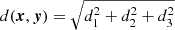 , with di = min{|xi − yi|,Li − |xi − yi|}. This is applicable if r is smaller than any Li/2. For the shifted periodic box, we have Wx = {y | y − x ∈ W}=W and consequently the (isotropised) set-covariance is constant
  . Similar to the derivation in Eq. (A.4), the expectation value of DD(r) can be calculated using the Campbell-Mecke formula:
![Mathematical equation: $$ \begin{aligned} {\mathbb{E} }[\mathsf{DD }(r)]&= \frac{4\pi }{N^2} \int _{r}^{r+{\delta }}\!\! |{W}|\, \varrho ^2 (1+\xi (s))\, s^2{\mathrm{d} }s \nonumber \\&= \frac{|S_r^{\delta }|}{|{W}|} + \frac{4\pi }{|{W}|} \int _{r}^{r+{\delta }}\!\! \xi (s)\, s^2{\mathrm{d} }s \nonumber \\&\approx \ \frac{4\pi r^2 {\delta }}{|{W}|} (1 + \xi (s)) \quad \mathrm{for}\; {\delta }\; \mathrm{small}, \end{aligned} $$](/articles/aa/full_html/2022/10/aa43632-22/aa43632-22-eq115.gif) (A.11)
(A.11)
where the volume of the shell  . Therefore, for small δ,
  is an unbiased estimate of the two-point correlation function ξ(r) in a periodic box; neither a random points set, nor a boundary correction with geometric factors is needed.
A.2. Expectation of pair-counts for inhomogeneous point sets
As described in Sect. 6 we are naturally confronted with an inhomogeneous sampled galaxy distribution. Here we calculate the expectation values of DD′,DR′ and RR′ for such an inhomogeneous situation.
One also has Campbell-Mecke formulas for an inhomogeneous point process Φ′ (Baddeley et al. 2000; Shaw et al. 2021):
![Mathematical equation: $$ \begin{aligned} {\mathbb{E} }\left[\sum _{\boldsymbol{x}\in \Phi \prime } f(\boldsymbol{x})\,\right]&= \int _{{\mathbb{R} }^3}f(\boldsymbol{x})\, \varrho \prime (\boldsymbol{x})\, {\mathrm{d} }{\boldsymbol{x}},\end{aligned} $$](/articles/aa/full_html/2022/10/aa43632-22/aa43632-22-eq118.gif) (A.12)
(A.12)
![Mathematical equation: $$ \begin{aligned} {\mathbb{E} }\left[\sum _{\begin{matrix} {\boldsymbol{x}},{\boldsymbol{y}}\in \Phi \prime \\ {\boldsymbol{x}}\ne {\boldsymbol{y}} \end{matrix}} g(\boldsymbol{x},\boldsymbol{y})\,\right]&= \int _{{\mathbb{R} }^3}\int _{{\mathbb{R} }^3} g(\boldsymbol{x},\boldsymbol{y})\, \varrho _2\prime (\boldsymbol{x},\boldsymbol{y})\, {\mathrm{d} }{\boldsymbol{x}}{\mathrm{d} }{\boldsymbol{y}} \\&= \int _{{\mathbb{R} }^3}\int _{{\mathbb{R} }^3} g(\boldsymbol{x},\boldsymbol{y})\,\varrho \prime (\boldsymbol{x})\varrho \prime (\boldsymbol{y})\,(1+\xi^\prime (|\boldsymbol{x}-\boldsymbol{y}|))\, {\mathrm{d} }{\boldsymbol{x}}{\mathrm{d} }{\boldsymbol{y}}.\nonumber \end{aligned} $$](/articles/aa/full_html/2022/10/aa43632-22/aa43632-22-eq119.gif) (A.13)
(A.13)
Again we consider
 (A.14)
and calculate the expectation (see Baddeley et al. 2000; Shaw et al. 2021 for similar derivations)
![Mathematical equation: $$ \begin{aligned} &{{\mathbb{E} }[S^\prime ] = \int _{{\mathbb{R} }^3}\!\int _{{\mathbb{R} }^3}\!\! {\mathbb{1} }_{W}(\boldsymbol{x}) {\mathbb{1} }_{W}(\boldsymbol{y}) {\delta }k_r^{\delta }(|\boldsymbol{x}-\boldsymbol{y}|) \varrho _2\prime (|\boldsymbol{x}-\boldsymbol{y}|)\, {\mathrm{d} }{\boldsymbol{x}}{\mathrm{d} }{\boldsymbol{y}}} \\ &\quad\ \ = \int _{{\mathbb{R} }^3}\! \int _{{\mathbb{R} }^3}\!\! {\mathbb{1} }_{W}(\boldsymbol{z}+\boldsymbol{y}) {\mathbb{1} }_{W}(\boldsymbol{y}) \varrho \prime (\boldsymbol{z}+\boldsymbol{y})\varrho \prime (\boldsymbol{y}) {\mathrm{d} }{\boldsymbol{y}}\ {\delta }k_r^{\delta }(|\boldsymbol{z}|) (1+\xi^\prime (|\boldsymbol{z}|) {\mathrm{d} }{\boldsymbol{z}} \\&\quad\ \ = 4\pi \int _{r}^{r+{\delta }}\!\! \overline{\Gamma }_{W}(s)\ (1+\xi^\prime (s))\ s^2{\mathrm{d} }s, \end{aligned} $$](/articles/aa/full_html/2022/10/aa43632-22/aa43632-22-eq121.gif) (A.15)
(A.15)
where  is the density weighted isotropised set-covariance
 (A.16)
For a homogeneous point distribution with 𝜚′(x) = 𝜚, we consistently get  .
.
The random point set used in RR′ is a realisation of an inhomogeneous Poisson process with number density  , and a vanishing two-point correlation function ξ′(r) = 0. N is the number of galaxies and Nr the number of random points in W. From Eq. (A.15) we get
![Mathematical equation: $$ \begin{aligned} {\mathbb{E} }[\mathsf{RR }^\prime (r)] = {\mathcal{RR} }^\prime (r)&= \frac{4\pi }{N^2} \int _{r}^{r+{\delta }} \overline{\Gamma _{W}}(s) \ s^2{\mathrm{d} }s \\&\approx \frac{4\pi r^2 {\delta }}{N^2}\ \overline{\Gamma _{W}}(r) \quad \mathrm{for}\; {\delta }\; \mathrm{small}.\nonumber \end{aligned} $$](/articles/aa/full_html/2022/10/aa43632-22/aa43632-22-eq126.gif) (A.17)
(A.17)
Using Eq. (A.15) and Eq. (A.17) we can determine
![Mathematical equation: $$ \begin{aligned} \frac{{\mathbb{E} }[\mathsf{DD }^\prime (r)]}{{\mathbb{E} }[\mathsf{RR }^\prime (r)]}&= \frac{\int _{r}^{r+{\delta }} \overline{\Gamma _{W}}(s)\ (1+\xi^\prime (s)) s^2{\mathrm{d} }s}{\int _{r}^{r+{\delta }} \overline{\Gamma _{W}}(s)\ s^2{\mathrm{d} }s}\nonumber \\&\approx 1 + \xi^\prime (r) \quad \mathrm{for}\; {\delta }\;\mathrm{small},\nonumber \end{aligned} $$](/articles/aa/full_html/2022/10/aa43632-22/aa43632-22-eq127.gif)
Hence we arrive at the well-known result that the estimator  of Peebles & Hauser (1974) is ‘ratio unbiased’.
  is an estimate of the two-point correlation function ξ′(r) = ξG(r) if we apply the same selection effects to the random point set as we find in the incompletely sampled galaxy distribution.
For a given point set  inside the sample geometry xi ∈ W, we calculate the expectation of DR′. Using the Campbell-Mecke formula and with Φ′ an inhomogeneous Poisson process with number density
  , we obtain
![Mathematical equation: $$ \begin{aligned} {\mathbb{E} }[\mathsf{DR }^\prime ]&= {\mathcal{DR} }^\prime (r) = \frac{1}{N{{N_{\rm r}}}} \sum _{i=1}^N \int _{{\mathbb{R} }^3} {\mathbb{1} }_{W}(\boldsymbol{y})\, {\delta }k_r^{\delta }(|{\boldsymbol{x}}_i-\boldsymbol{y}|)\, \tfrac{{{N_{\rm r}}}}{N}\varrho \prime (\boldsymbol{y})\, {\mathrm{d} }{\boldsymbol{y}}\nonumber \\&= \frac{1}{N^2} \sum _{i=1}^N {\mathcal{U} }_r^{\delta }({\boldsymbol{x}}_i), \end{aligned} $$](/articles/aa/full_html/2022/10/aa43632-22/aa43632-22-eq132.gif) (A.18)
(A.18)
where
 (A.19)
is the integral of the density 𝜚′(y) in the volume of the spherical shell  inside W.
Appendix B: Simple windows
The area fraction area(∂Br(x)∩W) and the (isotropised) set covariance  can be calculated for a rectangular box W. We use these expressions to determine the accuracy of the (quasi-) Monte Carlo integration schemes. We also reiterate the result for a sphere and for two-dimensions.
B.1. Rectangular box
For a point x = (x1, x2, x3)T and a rectangular box W = [0, L1]×[0, L2]×[0, L3] with side lengths L1 > |x1|,L2 > |x2|,L3 > |x3|, the set–covariance is
 (B.1)
(B.1)
and the isotropised set-covariance is for r < min{L1, L2, L3}
 (B.2)
(B.2)
(see e.g. Stoyan & Stoyan 1994; Kerscher 1999). A simple integration gives us the integrated isotropised set-covariance:
 (B.3)
(B.3)
which we need to calculate ℛℛ(r) according to Eq. (A.5).
It is more involved to calculate the surface area of a sphere inside a rectangular box W. Using the inclusion-exclusion formula, Baddeley et al. (1993) derive an explicit expression for the area fraction area(∂Br(x)∩W):
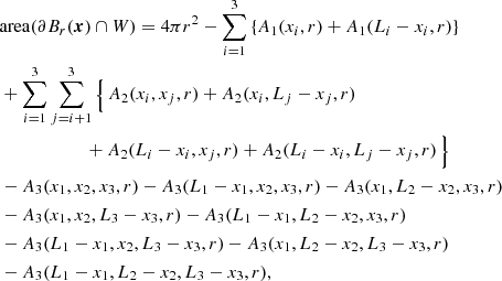 (B.4)
(B.4)
with
 (B.5)
(B.5)
The following expression for C(a, b, c) is almost the same as Eq. (37) from Baddeley et al. (1993), but with two typos corrected. These correct results have already been used in the spatstat package for R (Baddeley & Turner 2005; see sphefrac.c for the implementation). For a, b, c > 0 and a2 + b2 + c2 < 1, we get
 (B.6)
(B.6)
For a2 + b2 + c2 ≥ 1, we have C(a, b, c) = 0. As special cases,
 (B.7)
(B.7)
and  .
.
B.2. Sphere
For a spherical sample W = BR centred at the origin with radius R and with r = |x|< R, the set-covariance reads
 (B.8)
(B.8)
Due to symmetry, the isotropised set-covariance is simply  . The area fraction for a point q ∈ W at a distance |q|=s > R − r from the origin, and with r < R is area(∂Br(q)∩W) = 4 α r2, with
  .
.
B.3. Two dimensions
Here we give the expressions for the set-covariance in two dimensions. For a point x = (x1, x2)T ∈ ℝ2 and a rectangle W = [0, L1]×[0, L2] with side lengths L1 > |x1|,L2 > |x2|, the set–covariance is
 (B.9)
(B.9)
and for r < min{L1, L2}, the isotropised set-covariance is (Ripley 1988)
 (B.10)
The analogue to area(∂Br(x)∩W) is the arc-length arc(Cr(x)∩W) of the circumference of a circle Cr(x) with radius r centred on a point x ∈ W inside the sample window W. It can be calculated from the intersection points of the circle with the sides of W and the angles between them and the centre (Stoyan et al. 1995).
Appendix C: Implementation and run time
We use Python with NumPy (Harris et al. 2020) and SciPy (Virtanen et al. 2020) to implement the data processing, calculate geometric quantities, generate random points, and to generate randomised Halton sequences (provided in SciPy starting with version ≥1.7.0). The performance critical parts are the pair-counting and a function for checking whether or not points are inside the observational window. We implemented these routines as C++ functions parallelised using OpenMP (Dagum & Menon 1998). They are made callable from Python via pybind11 (Jakob et al. 2017). In the computations of DD and RR, we obviously avoid the double counting by using ∑i∑j ≠ i… = 2∑i∑j > i…⋅ We implement the double sums without using a tree, resulting in a code with a run time quadratic in the number of points (see below). Using OpenMP, we could achieve a reduction of the computing time almost linear with the number of computing cores used (at least up to the 20 cores we were able to access; see also Alonso 2012). Only these optimisations are included in our code but perhaps it is versatile enough to help with future implementations3.
C.1 Run time
As initial guidance, the run time of the pair-count calculations should scale with the number of distance calculations actually performed. This again depends on the number of (quasi-)random or data points, and on the data structure and algorithm used. With our direct implementation of the double sums from eqs. (2), (5), (6), (16) we expect the run time to scale as TDD ∝ N2, TDR ∝ NNr, TRR ∝  and TRR, 2x3d ∝
  , respectively. This is independent of the number of radius intervals, because we can sort the counts into the corresponding radius bin. The calculation of DRshell should scale as TDR, shell ∝ NNsh, but we need to repeat the pair-count calculation for each radius bin. One could envision optimising this for convex windows.
To estimate the run time, we ran our mildly optimised code on a current small workstation equipped with an Intel Xeon W1350 processor with six cores and a clock frequency of at least 3.3 GHz. Memory was not an issue in these calculations. As expected, we see from Fig. C.1 that for large Nr, the run time of RR and RR2x3d grows quadratically with Nr, and that RR2x3d is slower than RR by a factor of two. The run time of DR and DRshell shows the expected linear scaling with Nr. At fixed Nr and N, the run time of DRshell is more than one order of magnitude longer than DR. But we note that for fixed accuracy we need significantly less quasi-random points in DRshell. We also consider subsamples with N = 1000 and N = 100 data points from the N = 10429 clusters and confirm the linear scaling of TDR and TDR, shell with N. We find the same results for r ∈ [30, 35] Mpc h−1 and r ∈ [100, 105] Mpc h−1.
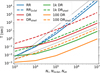 |
Fig. C.1. Run time of the pair-counts for r ∈ [5, 10] Mpc h−1 and W = [0, 1]3. The black dotted lines are proportional to Nr and |

In all our calculations, we used a parallelised direct double sum implementation to calculate the pair-counts. As already mentioned, a significant speedup can be expected if one uses tree-based methods (Moore et al. 2001). To illustrate this, we compare the run time of our parallelised pair-count implementation for RR to an implementation using the kd–tree provided with SciPy (KDTree). As the direct double sum implementation ran parallelised and the KDTree on a single core, the absolute run times are not comparable, but the scaling with Nr is the essential result. The direct implementation shows the expected scaling ∝  of the run time in Fig. C.2. For the tree-based method, we observe that for small radii the run time scales with ∝Nrlog(Nr) and a significant speedup can be achieved. However, for large radii, the run time scales ∝
  , comparable to the direct implementation. In a similar comparison for the window [0, 1]×[0, 0.1]2 the run time of the tree based method scales ∝
  for all radii. We therefore confirm a significant speedup for tree-based methods, especially in voluminous samples and for small radii. Tree-based methods, or the other computational optimisations mentioned in the introduction, can be applied directly to DD, RR, DR, and RR2x3d, and should speedup these calculations further. Whether or not similar optimisation schemes can be found for DRshell is an open question.
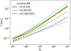 |
Fig. C.2. Run time of RR in [0, 1]3 for the direct double sum implementation (three solid lines, almost on top of each other), and the implementation using KDTree (dashed lines). The black dotted lines are proportional to Nrlog(Nr) and |

For a given point set and window there is plenty of scope for optimising the run times. However, such an optimisation problem easily turns into a multi-parameter endeavour. The run time not only depends the accuracy goal, the radius, the bin width, and the density of the point set but also on the hardware platform, the operating system, the algorithms, the data structures, the details of the implementation, and so on.
All Tables
All Figures
|
Fig. 1. Relative error εRR against the number of random points Nr used in the standard procedure for calculating RR(r) in rectangular windows W. The black dotted lines are proportional to 1/Nr and |
| In the text | |
|
Fig. 2. Relative error εRR, 2x3d calculated for rectangular windows W with a pure Monte Carlo integration (solid lines) and with a randomised Halton sequence (dashed lines). The black dotted lines are proportional to |
| In the text | |
|
Fig. 3. Relative error εDR calculated for rectangular windows W with a standard Monte Carlo integration (solid lines) and with a quasi-Monte Carlo scheme using a randomised Halton sequence (dashed lines). The black dotted lines are proportional to |
| In the text | |
|
Fig. 4. Relative error εDR, shell calculated for rectangular windows W with a pure Monte Carlo integration (solid lines) and with a randomised Halton sequence (dashed lines). The black dotted lines are proportional to |
| In the text | |
|
Fig. 5. Two-point correlation function calculated for a simulated galaxy cluster sample. The exact Ξ is compared to standard ξLS with Nr = 104 and Nr = 105 random points, and to the new |
| In the text | |
|
Fig. 6. Absolute error Δ1 is shown for the standard RR (solid lines) and for RR2x3d (dashed lines) pair-counts. The black dotted lines are proportional to |
| In the text | |
|
Fig. 7. Absolute error Δ2 is shown for the standard DR (solid lines), the DR using a low-discrepancy sequence (dotted lines), and for DRshell also using a low-discrepancy sequence (dashed lines). The black dotted lines are proportional to |
| In the text | |
|
Fig. 8. Errors for estimates of the correlation function at r ∈ [2, 3] Mpc h−1 from 1.36 million galaxies and a subsample of 100 k galaxies in a box with side-length 325 Mpc h−1. Upper plot: absolute error Δ1 shown for the standard RR (solid lines) and for RR2x3d (dashed lines) pair-counts. Lower plot: absolute error Δ2 is shown for the standard DR (solid lines), the DR using a low-discrepancy sequence (dotted lines), and for DRshell also using a low-discrepancy sequence (dashed lines). The black dotted lines are proportional to |
| In the text | |
|
Fig. C.1. Run time of the pair-counts for r ∈ [5, 10] Mpc h−1 and W = [0, 1]3. The black dotted lines are proportional to Nr and |
| In the text | |
|
Fig. C.2. Run time of RR in [0, 1]3 for the direct double sum implementation (three solid lines, almost on top of each other), and the implementation using KDTree (dashed lines). The black dotted lines are proportional to Nrlog(Nr) and |
| In the text | |
Current usage metrics show cumulative count of Article Views (full-text article views including HTML views, PDF and ePub downloads, according to the available data) and Abstracts Views on Vision4Press platform.
Data correspond to usage on the plateform after 2015. The current usage metrics is available 48-96 hours after online publication and is updated daily on week days.
Initial download of the metrics may take a while.