© E. Keihänen et al. 2022

1. Introduction

The next generation of telescopes for cosmology surveys, such as Euclid (Laureijs et al. 2011), the Vera Rubin Observatory (Ivezić et al. 2019), DESI (DESI Collaboration 2016), or the Nancy Grace Roman Space Telescope (Akeson et al. 2019), will soon greatly improve the quality and quantity of data for galaxy clustering and lensing measurements. Their main aim is to illuminate the dark sector of cosmology, to test Einstein’s gravity on large scales, and to find signatures of the physics of inflation such as primordial non-Gaussianities.

Galaxy clustering is one of our most powerful cosmological probes (Cole et al. 2005; Eisenstein et al. 2005; Alam et al. 2005; Alam et al. 2021). However, galaxies are biased tracers of the nonlinear density field and their selection is subject to several different effects, such as fluctuations in exposure time, noise level, Milky Way extinction, photometry calibration error, sample contamination among others (e.g., Jasche & Lavaux 2017; Monaco et al. 2019; Kalus et al. 2019; Merz et al. 2021). Thus, their clustering will contain entangled information of matter clustering, galaxy bias, and observational systematics. The uncertainty will be represented by a covariance matrix. The inverse of the covariance matrix, the precision matrix, will be used in the likelihood analysis to infer cosmological parameters and their covariance. An accurate quantification of the clustering covariance under all the sources of uncertainty is therefore of paramount importance for the success of a survey.

It is customary to construct covariance matrices of galaxy clustering by using large samples of hundreds, if not thousands, of mock galaxy catalogs in the past light cone (e.g., Manera et al. 2013; Kitaura et al. 2016). Any known selection effects are applied to the mock catalogs, after which the clustering signal is measured with the same procedure as the one used for the actual data catalog. This sample of clustering measurements makes it possible to construct a brute-force numerical sample covariance. This approach has many advantages. It is conceptually simple, and the covariance built this way is positive-definite by construction. The estimation error of the covariance and its propagation to parameter estimation are well understood (Taylor et al. 2013; Taylor & Joachimi 2014; Hartlap et al. 2007; Dodelson & Schneider 2013; Percival et al. 2014, 2022; Sellentin & Heavens 2016). The sample covariance, however, is computationally expensive to construct; the variance of the covariance estimate decreases proportionally to 1/N, where N is the number of simulations, so getting the error down to a 10% level requires about 100 independent realizations, and ∼10 000 realizations for a 1% level.

This raises two related problems: on the one hand, the production of such mocks, which are typically addressed with approximate methods to bypass the high cost of N-body simulations (Monaco 2016); on the other hand, the measurement of galaxy clustering of thousands of mocks, which can be a bottleneck for a processing pipeline. Several strategies have been proposed to reduce the cost of covariance estimation. These include precision matrix expansion (Friedrich & Eifler 2018), tapering (Paz & Sánchez 2015), eigenvalue decomposition (Gaztañaga & Scoccimarro 2005), linear shrinkage (Pope & Szapudi 2008), sparse precision matrix estimation (Padmanabhan et al. 2016), and nonlinear shrinkage (Joachimi 2017).

In this work we focus on the estimation of the two-point correlation function (2PCF) and its covariance. In the special case of Gaussian fluctuations, the 2PCF contains all information on the statistical properties of the galaxy distribution. A concrete example would be the European Space Agency’s Euclid cosmology mission, and in particular its spectroscopic sample of Hα emitting galaxies (Euclid Collaboration 2022). This galaxy sample is expected to be as large as 20–30 million galaxies in the redshift range 0.9–1.8. The Euclid Consortium plans to represent the covariance matrix of the 2PCF with a few thousand mock catalogs. The time needed to measure the 2PCF of such a large number of mocks will be one major contributor to the whole pipeline from raw images to cosmological parameter inference.

The Landy–Szalay estimator (Landy & Szalay 1993) has become the standard estimator in galaxy clustering science. In addition to the actual galaxy catalog, the Landy–Szalay estimator requires a random catalog, which represents a uniform distribution of points within the survey volume considered, modulated with same weighting and selection as the data catalog. The 2PCF is then built as a combination of data-data (DD), data-random (DR), and random-random (RR) pair counts. The estimator is unbiased at the limit of an infinite random catalog, and, when the fluctuations are small, it yields the minimum-variance solution for the correlation function.

Since the random catalog is usually much larger (in number of objects) than the data catalog, the computational cost of the estimator is dominated by the cost of the RR counts. Glass-like random catalogs (Dávila-Kurbán et al. 2021) have been proposed as a way of reducing the required random catalog size. A straightforward way to reduce the cost is to coadd RR pair counts from a collection of small subcatalogs, rather than counting the pairs in one large catalog, thus omitting pairs between subcatalogs. This natural idea has been applied in many studies without explicit mention, or without assigning a name to it. We refer to this approach as the “split” method, thusly named because of the idea of “splitting” a large random catalog into several small ones. The term was coined in Keihänen et al. (2019), where the effect of the size of the random catalog on the estimator error is studied in a systematic way, and it is shown that the effect of the splitting on the estimation error is negligible. It is also shown that the optimal relation between the accuracy and computational cost is achieved when the subcatalogs have the same number of objects as the data catalog.

Even with a split random catalog, most of the computation time goes into the counting of the RR and DR pairs, while the estimation error is dominated by the scatter of the data points. The same applies to the sampling of the covariance matrix, the cost of which is N times that of a single 2PCF estimation. Using a single random catalog for all measurements can reduce the cost of the RR counts, but then counting the DR pairs becomes the next bottleneck.

In this paper we introduce a way of speeding up the covariance estimation, specific to the Landy–Szalay estimator. We aim to show that the covariance matrix for a 2PCF estimate can be constructed using a significantly smaller random catalog than what was used in the construction of the 2PCF itself.

The paper is organized as follows. In Sect. 2 we present the method and its theoretical background. In Sect. 3 we discuss the accuracy of the method, derive a covariance of covariance, and discuss implications for parameter estimation. In Sect. 4 we describe the simulations we used for the validation of the method. In Sect. 5 we present our results, comparing the accuracy and speed of the new method to those of the sample covariance. We give our conclusions in Sect. 6.

This work has made use of the 2PCF code developed by the Euclid Consortium.

2. Method

2.1. Landy–Szalay estimator

We denote the number of objects in the data catalog by N_d, and in the random catalog by N_r. We assume that the two-point correlation function is estimated with the Landy–Szalay estimator, with the additional twist of the “split” option, as follows. The random catalog is split into M subcatalogs, where M is called the split factor. RR pairs are counted within each subcatalog and coadded, but pairs of objects in two distinct subcatalogs are omitted. Each subcatalog will have to obey the same statistical properties and have the same sky coverage as the full catalog. In other words, each subcatalog must itself be a valid random catalog. Splitting the random catalog reduces the computational cost of 2PCF estimation significantly, for a negligible loss of accuracy (Keihänen et al. 2019). The optimal split factor has been shown to be M = N_r/N_d, that is to say the random catalog is split into subcatalogs of the same size as the data catalog. For fixed N_r, this minimizes the variance of the correlation function for a given computation time, or minimizes the computation time required to reach a given target variance. From here on we parametrize the size of the random catalog as N_r = MN_d.

The random catalog is usually constructed to be significantly larger than the data catalog, in order that the estimation error is dominated by the scatter of the data points rather than that of the random points. In this work we use as baseline the value M = 50, the value adopted for the Euclid galaxy clustering study.

The Landy–Szalay estimator is

$$\begin{array}{c}\hfill \widehat{\xi }(\mathbf{r}):=\frac{\mathrm{dd}(\mathbf{r})-2\mathrm{dr}(\mathbf{r})}{\mathrm{rr}(\mathbf{r})}+1,\end{array}$$(1)

where dd(r), dr(r), and rr(r) denote the normalized data-data, data-random, and random-random pair counts in a separation bin. Following the notation of Keihänen et al. (2019), we use the vector r to denote the generalized separation vector. Vector r may refer to a physical separation distance, or, more generally, to an arbitrary bin in 1D, 2D, or 3D space. The normalized data-data pair count is

$$\begin{array}{c}\hfill \mathrm{dd}(\mathbf{r}):=\frac{\mathrm{DD}(\mathbf{r})}{N_{\mathrm{d}}(N_{\mathrm{d}}-1)/2},\end{array}$$(2)

where DD(r) is the unnormalized pair count. This is unaffected by the split. Similarly, the normalized data-random count is given by

$$\begin{array}{c}\hfill \mathrm{dr}(\mathbf{r}):=M^{-1}{\displaystyle \sum _{i=1}^M\frac{{\mathrm{DR}}_i(\mathbf{r})}{N_{\mathrm{d}}^2}=M^{-1}\sum _{i=1}^M{\mathrm{dr}}_i(\mathbf{r}),}\end{array}$$(3)

where DR_i is the pair count between the data catalog and the ith random subcatalog. Since the dependence on the random catalog is linear, this too is unaffected by the split.

The normalized random-random count with split can be written as

$$\begin{array}{c}\hfill \mathrm{rr}(\mathbf{r}):=M^{-1}{\displaystyle \sum _{i=1}^M\frac{{\mathrm{RR}}_i(\mathbf{r})}{N_{\mathrm{d}}(N_{\mathrm{d}}-1)/2}=M^{-1}\sum _{i=1}^M{\mathrm{rr}}_i(\mathbf{r}),}\end{array}$$(4)

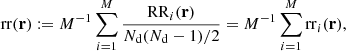
where RR_i is the unnormalized pair count from the ith subcatalog. With this notation, the split Landy–Szalay estimator becomes

$$\begin{array}{c}\hfill \widehat{\xi }(\mathbf{r})=\frac{\mathrm{dd}(\mathbf{r})-\frac{2}{M}{\sum }_i{\mathrm{dr}}_i(\mathbf{r})}{M^{-1}{\sum }_i{\mathrm{rr}}_i(\mathbf{r})}+1.\end{array}$$(5)

We use the hat ($\widehat{\xi }$) to indicate that this is an estimate of the true correlation function ξ.

The computational cost of the estimator is roughly proportional to the total number of pairs counted. The cost of the split estimator is proportional to $\frac{1}{2}{N}_{{}_{\mathrm{d}}}^2(1+3M)$, while without split the cost grows proportional to $\frac{1}{2}{N}_{{}_{\mathrm{d}}}^2(1+2M+M^2)$.

2.2. Covariance

We consider the estimated correlation function in two distance bins r₁ and r₂, which may or may not be the same. We want to estimate the covariance

$$\begin{array}{c}\hfill \mathrm{cov}[\widehat{\xi }({\mathbf{r}}_1),\widehat{\xi }({\mathbf{r}}_2)]:=\langle [\widehat{\xi }({\mathbf{r}}_1)-⟨\widehat{\xi }({\mathbf{r}}_1)⟩][\widehat{\xi }({\mathbf{r}}_2)-⟨\widehat{\xi }({\mathbf{r}}_2)⟩]\rangle .\end{array}$$(6)

The brackets ⟨⟩ denote an average over an infinite ensemble of data realizations, for fixed cosmology and survey geometry. Since we consider the actual measured correlation function to represent one such realization, the covariance is a measure of the statistical uncertainty in the measured correlation function.

Assume we have N mock catalogs and corresponding random catalogs, with the same sky coverage, masking etc. as the actual survey catalog. Let ${\widehat{\xi }}_i(\mathbf{r}),i=1\dots N$ denote the set of correlation functions estimated from these mocks. An unbiased estimate of the covariance is given by the sample covariance

$$\begin{array}{c}\hfill \widehat{\mathcal{C}}[\widehat{\xi }({\mathbf{r}}_1),\widehat{\xi }({\mathbf{r}}_2)]:=\frac{1}{N-1}{\displaystyle \sum _{i=1}^N[{\widehat{\xi }}_i({\mathbf{r}}_1)-\overline{\xi }({\mathbf{r}}_1)][{\widehat{\xi }}_i({\mathbf{r}}_2)-\overline{\xi }({\mathbf{r}}_2)],}\end{array}$$(7)

where

$$\begin{array}{c}\hfill \overline{\xi }(\mathbf{r}):=\frac{1}{N}{\displaystyle \sum _{i=1}^N}{\widehat{\xi }}_i(\mathbf{r})\end{array}$$(8)

is the estimated mean. The required number of mocks will depend on the accuracy requirement of the application in question. For few percent-level accuracy in parameter error bars, N ≳ 1000 is required.

Throughout this paper we use a convention where the symbol $\widehat{\text{C}}$ with a hat denotes a numerical estimate of a covariance, and either cov or C denotes the true (ensemble average) covariance. Specifically, $\widehat{\mathcal{C}}$ is reserved for the sample covariance estimate, constructed as in Eq. (7) (see Table 1).

The computational cost of constructing the sample covariance, obviously, is N times the cost of a single 2PCF estimate. In this paper we show that a given level of accuracy can be reached with a significantly lower CPU cost. For this goal, we now break the covariance of the Landy–Szalay estimator into pair count covariances.

Following the notation of the Landy–Szalay paper, we write

$$\begin{array}{cc}& \mathrm{dd}(\mathbf{r})=⟨\mathrm{dd}(\mathbf{r})⟩[1+\alpha (\mathbf{r})],\hfill \\ \hfill & {\mathrm{dr}}_i(\mathbf{r})=⟨\mathrm{dr}(\mathbf{r})⟩[1+{\beta }_i(\mathbf{r})],\hfill \\ \hfill & {\mathrm{rr}}_i(\mathbf{r})=⟨\mathrm{rr}(\mathbf{r})⟩[1+{\gamma }_i(\mathbf{r})].\hfill \end{array}$$(9)

The brackets ⟨⟩ indicate an ensemble average. Thus α, β_i, γ_i capture the variation of the pair counts around their average. By definition, ⟨α⟩ = ⟨β⟩ = ⟨γ⟩ = 0. Inserting these into the Landy–Szalay estimator yields

$$\begin{array}{cc}& \widehat{\xi }(\mathbf{r})=\frac{⟨\mathrm{dd}(\mathbf{r})⟩[1+\alpha (\mathbf{r})]}{⟨\mathrm{rr}(\mathbf{r})⟩[1+M^{-1}{\sum }_i{\gamma }_i(\mathbf{r})]}\hfill \\ \hfill & -2\frac{⟨\mathrm{dr}(\mathbf{r})⟩[1+M^{-1}{\sum }_i{\beta }_i(\mathbf{r})]}{⟨\mathrm{rr}(\mathbf{r})⟩[1+M^{-1}{\sum }_i{\gamma }_i(\mathbf{r})]}+1.\hfill \end{array}$$(10)

For the ensemble averages it holds that ⟨dr(r)⟩ = ⟨rr(r)⟩ and ⟨dd(r)⟩ = d(r)⟨rr(r)⟩, where we define

$$\begin{array}{c}\hfill d(\mathbf{r}):=1+\xi (\mathbf{r}).\end{array}$$(11)

If the RR counts are large, as is usually the case, then γ_i(r)≪1, and [1 + M⁻¹∑_iγ_i(r)]⁻¹ ≈ 1 − M⁻¹∑_iγ_i(r). Assuming α, β, γ ≪ 1, we can drop the quadratic terms, and the estimator becomes

$$\begin{array}{cc}& \widehat{\xi }(\mathbf{r})\approx d(\mathbf{r})[1+\alpha (\mathbf{r})-M^{-1}{\sum }_i{\gamma }_i(\mathbf{r})]\hfill \\ \hfill & -2[1+M^{-1}{\sum }_i{\beta }_i(\mathbf{r})-M^{-1}{\sum }_i{\gamma }_i(\mathbf{r})]+1\hfill \end{array}$$(12)

and as ensemble average 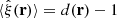$⟨\widehat{\xi }(\mathbf{r})⟩=d(\mathbf{r})-1$. The deviation from the ensemble average is

$$\begin{array}{cc}& \widehat{\xi }(\mathbf{r})-⟨\xi (\mathbf{r})⟩\hfill \\ \hfill & \approx d(\mathbf{r})[\alpha (\mathbf{r})-M^{-1}{\sum }_i{\gamma }_i(\mathbf{r})]-2M^{-1}[{\sum }_i{\beta }_i(\mathbf{r})-{\sum }_i{\gamma }_i(\mathbf{r})].\hfill \end{array}$$(13)

Inserting Eq. (13) into Eq. (6) yields a combination of cross-correlation terms between α, β, γ. We now consider each of them in turn, and make use of our knowledge of their statistical properties to calculate the expectation values.

Let us begin with the term

$$\begin{array}{c}\hfill M^{-2}{\displaystyle \sum _{\mathit{ij}}}⟨{\gamma }_i({\mathbf{r}}_1){\gamma }_j({\mathbf{r}}_2)⟩.\end{array}$$(14)

Indices i, j label independent random subcatalogs, all of which are statistically identical. We therefore have ⟨γ_i(r₁)γ_j(r₂)⟩ = 0 for i ≠ j, and ⟨γ_i(r₁)γ_i(r₂)⟩ = ⟨γ(r₁)γ(r₂)⟩, where we drop the subscript to indicate an ensemble average that is the same for all subcatalogs. The covariance element becomes

$$\begin{array}{c}\hfill M^{-2}{\displaystyle \sum _{\mathit{ij}}⟨{\gamma }_i({\mathbf{r}}_1){\gamma }_j({\mathbf{r}}_2)⟩=M^{-1}⟨\gamma ({\mathbf{r}}_1)\gamma ({\mathbf{r}}_2)⟩.}\end{array}$$(15)

Based on similar arguments we can write

$$\begin{array}{c}\hfill M^{-1}{\displaystyle \sum _i}⟨\alpha ({\mathbf{r}}_1){\beta }_i({\mathbf{r}}_2)⟩=⟨\alpha ({\mathbf{r}}_1)\beta ({\mathbf{r}}_2)⟩\end{array}$$(16)

and

$$\begin{array}{c}\hfill M^{-1}{\displaystyle \sum _i⟨\alpha ({\mathbf{r}}_1){\gamma }_i({\mathbf{r}}_2)⟩=⟨\alpha ({\mathbf{r}}_1)\gamma ({\mathbf{r}}_2)⟩.}\end{array}$$(17)

Assuming that the random catalog and the data catalog are independent would allow us to drop the ⟨α(r₁)γ_i(r₂)⟩ terms. This is however not necessarily always true. If the characteristics of the observed data catalog (mask, selection function) are used for the generation of the random catalog, a correlation may arise between the data catalog and the random catalog. Although such correlations are likely to be small, the assumption of independence is not relevant for the method we are developing, and we will thus not implement it.

When dealing with the terms involving β and γ, we split the sums into i = j and i ≠ j parts, to obtain

$$\begin{array}{cc}& M^{-2}{\displaystyle \sum _{\mathit{ij}}⟨{\beta }_i({\mathbf{r}}_1){\beta }_j({\mathbf{r}}_2)⟩}\hfill \\ \hfill & =M^{-1}⟨\beta ({\mathbf{r}}_1)\beta ({\mathbf{r}}_2)⟩+(1-M^{-1}){⟨\beta ({\mathbf{r}}_1)\beta ({\mathbf{r}}_2)⟩}_{\mathrm{cr}}.\hfill \end{array}$$(18)

Here the subscript cr (‘cross’) denotes that we are dealing with DR counts that involve two distinct random subcatalogs, however correlated through the shared data catalog.

Based on similar arguments, we obtain:

$$\begin{array}{cc}& M^{-2}{\displaystyle \sum _{\mathit{ij}}}⟨{\beta }_i({\mathbf{r}}_1){\gamma }_j({\mathbf{r}}_2)⟩\hfill \\ \hfill & =M^{-1}⟨\beta ({\mathbf{r}}_1)\gamma ({\mathbf{r}}_2)⟩+(1-M^{-1}){⟨\beta ({\mathbf{r}}_1)\gamma ({\mathbf{r}}_2)⟩}_{\mathrm{cr}}.\hfill \end{array}$$(19)

As in the case of ⟨αγ⟩, assuming independence between the random catalog and the data catalog would allow us to drop the second term, but this assumption is not relevant for the method under discussion.

We introduce a more concise notation, where we drop the arguments r₁ and r₂, and each term is interpreted as a symmetrized version of itself. When d is involved, it is paired with the first element. For instance, d⟨αβ⟩ is to be read as

$$\begin{array}{c}\hfill d⟨\alpha \beta ⟩=\frac{1}{2}[d({\mathbf{r}}_1)⟨\alpha ({\mathbf{r}}_1)\beta ({\mathbf{r}}_2)⟩+d({\mathbf{r}}_2)⟨\alpha ({\mathbf{r}}_2)\beta ({\mathbf{r}}_1)⟩],\end{array}$$(20)

similarly for the other pairs. In this notation, the covariance takes the form

$$\begin{array}{cc}& \mathrm{cov}[\widehat{\xi }({\mathbf{r}}_1),\widehat{\xi }({\mathbf{r}}_2);M]\hfill \\ \hfill & =d^2[⟨\alpha \alpha ⟩+M^{-1}⟨\gamma \gamma ⟩-2⟨\alpha \gamma ⟩]\hfill \\ \hfill & -4d[⟨\alpha \beta ⟩-⟨\alpha \gamma ⟩-M^{-1}⟨\gamma \beta ⟩-(1-M^{-1}){⟨\gamma \beta ⟩}_{\mathrm{cr}}+M^{-1}⟨\gamma \gamma ⟩]\hfill \\ \hfill & +4[M^{-1}⟨\beta \beta ⟩+(1-M^{-1}){⟨\beta \beta ⟩}_{\mathrm{cr}}\hfill \\ \hfill & -2M^{-1}⟨\beta \gamma ⟩-2(1-M^{-1}){⟨\beta \gamma ⟩}_{\mathrm{cr}}+M^{-1}⟨\gamma \gamma ⟩],\hfill \end{array}$$(21)

where the third argument (M) indicates the size of the random catalog.

We have expressed the Landy–Szalay covariance in terms of pair-count covariances. We are now arriving at an observation that is central for the method we are developing. Every term in Eq. (21) is either independent of M, or proportional to M⁻¹. The covariance is thus of the form

$$\begin{array}{c}\hfill \mathrm{cov}[\widehat{\xi }({\mathbf{r}}_1),\widehat{\xi }({\mathbf{r}}_2);M]=\mathrm{A}({\mathbf{r}}_1,{\mathbf{r}}_2)+\frac{1}{M}\mathrm{B}({\mathbf{r}}_1,{\mathbf{r}}_2).\end{array}$$(22)

Suppose we know the covariance for two distinct random-catalog sizes M = M_a and M = M_b > M_a. We readily see that Eq. (22) holds when

$$\begin{array}{cc}& \mathrm{A}({\mathbf{r}}_1,{\mathbf{r}}_2)=\frac{M_b}{M_b-M_a}\mathrm{cov}[\widehat{\xi }({\mathbf{r}}_1),\widehat{\xi }({\mathbf{r}}_2);M_b]\hfill \\ \hfill & -\frac{M_a}{M_b-M_a}\mathrm{cov}[\widehat{\xi }({\mathbf{r}}_1),\widehat{\xi }({\mathbf{r}}_2);M_a]\hfill \\ \hfill & \mathrm{B}({\mathbf{r}}_1,{\mathbf{r}}_2)=\frac{M_a{M}_b}{M_b-M_a}\{\mathrm{cov}[\widehat{\xi }({\mathbf{r}}_1),\widehat{\xi }({\mathbf{r}}_2);M_a]\hfill \\ \hfill & -\mathrm{cov}[\widehat{\xi }({\mathbf{r}}_1),\widehat{\xi }({\mathbf{r}}_2);M_b]\}.\hfill \end{array}$$(23)

To construct the covariance for an arbitrary value of M, it is sufficient to estimate the covariance for two smaller random-catalog sizes M_a and M_b. This is much cheaper than running the estimator with a large M. Equations (22) and (23) can then be used to construct the covariance for the actual random catalog size. This is the basic idea behind our proposed method.

2.3. Linear construction

We now consider how M_a and M_b should be chosen. The largest reduction in computational cost is obtained with M_a = 1 and M_b = 2. With M_b = M the method reduces to the conventional sample covariance.

We now argue in favor of selecting M_b = 2M_a. This allows us to use the random catalogs efficiently, as we now proceed to explain. For each mock data catalog we generate two independent random catalogs of same size M_a. We evaluate the M = M_a covariance with either of the two sets, and take the average. This is the M_a covariance to enter the formula (23). For the 2M_a covariance, we take the combined data of the two M_a random catalogs. This procedure reduces the scatter of the estimate, compared to generating a new 2M_a random catalog, since the correlated fluctuations cancel. We return to this point in Sect. 3 where we consider the accuracy of the estimated covariance quantitatively. To further save CPU time we save the DR and RR pair counts from the M = M_a simulations, and construct the M = 2M_a 2PCF from the saved pair counts, saving the CPU cost of another run with M = 2M_a. Throughout the rest of this paper we set M_b = 2M_a.

Our method is summarized formally as follows. We denote by ${\widehat{\text{C}}}_{\mathit{ij}}$ an estimated covariance matrix between two elements ξ(r_i),ξ(r_j) of the correlation function. Indices i, j may refer to different distance bins, or to elements picked from different multipoles.

We denote the correlation function estimated from a data catalog D and a random catalog R as $\widehat{\xi }(\mathrm{D},\mathrm{R})$, and the sample covariance over the set of mocks as ${\widehat{\mathcal{C}}}_{\mathit{ij}}(\widehat{\xi })$. We now have one data catalog D and two random catalogs R₁ and R₂, both of size M_a. We construct estimates for the covariances with M = M_a and M = 2M_a (which we denote by ${\widehat{\text{C}}}_{\mathit{ij}}^a$ and ${\widehat{\text{C}}}_{\mathit{ij}}^b$, respectively) as

$$\begin{array}{cc}& {\widehat{\mathrm{C}}}_{\mathit{ij}}^a:=\frac{1}{2}{\widehat{\mathcal{C}}}_{\mathit{ij}}\left[\widehat{\xi }(\mathrm{D},{\mathrm{R}}_1)\right]+\frac{1}{2}{\widehat{\mathcal{C}}}_{\mathit{ij}}\left[\widehat{\xi }(\mathrm{D},{\mathrm{R}}_2)\right]\hfill \\ \hfill & {\widehat{\mathrm{C}}}_{\mathit{ij}}^b:={\widehat{\mathcal{C}}}_{\mathit{ij}}\left[\widehat{\xi }(\mathrm{D},{\mathrm{R}}_1\cup {\mathrm{R}}_2)\right].\hfill \end{array}$$(24)

From these we construct two component matrices

$$\begin{array}{cc}& {\widehat{\mathrm{A}}}_{\mathit{ij}}:=2{\widehat{\mathrm{C}}}_{\mathit{ij}}^b-{\widehat{\mathrm{C}}}_{\mathit{ij}}^a\hfill \\ \hfill & {\widehat{\mathrm{B}}}_{\mathit{ij}}:=2M_a[{\widehat{\mathrm{C}}}_{\mathit{ij}}^a-{\widehat{\mathrm{C}}}_{\mathit{ij}}^b]\hfill \end{array}$$(25)

and the final covariance as

$$\begin{array}{c}\hfill {\widehat{\mathrm{C}}}_{\mathit{ij}}^{\mathrm{LC}}:={\widehat{\mathrm{A}}}_{\mathit{ij}}+M^{-1}{\widehat{\mathrm{B}}}_{\mathit{ij}}.\end{array}$$(26)

We refer to the covariance of Eq. (26) as the linear construction (LC) covariance.

The computational complexity of the Landy–Szalay estimator is roughly proportional to $\frac{1}{2}{N}_{\mathrm{d}}^2(1+3M)$, of which $\frac{1}{2}{N}_{\mathrm{d}}^2$ goes to DD pairs, $N_{\text{d}}^{2}M$ to DR pairs, and $\frac{1}{2}{N}_{\mathrm{d}}^{2}M$ to RR pairs. The cost of our proposed approach is $2·\frac{1}{2}{N}_{\mathrm{d}}^2(1+3M_a)$ per realization. This is assuming the 2PCF estimation code is run twice, which involves counting the DD pairs twice. If that is avoided, the cost is further reduced to $\frac{1}{2}{N}_{\mathrm{d}}^2(1+6M_a)$. With M = 50 and M_a = 1, the gain with respect to sample covariance is a factor of 151/7 ≈ 21.6, and increases with increasing M. Moreover, our result readily yields an extrapolation to infinite M, that is, we know what would be the estimator variance if we could use an infinite number of random points, and how much the variance with a finite M differs from that.

It is important to note that the presented derivation is based on very general assumptions on how the Landy–Szalay estimator is build from pair counts, and on the definition of variance. We do not make assumptions on the survey geometry, or which physical processes cause the scatter in the random counts, nor do we assume Gaussianity. The proposed method is thus valid for a very wide class of galaxy distributions.

Another important aspect to note is that the same procedure can be applied to any linear function of the correlation function. The only requirement is that the decomposition of Eq. (22) remains valid. In particular, the method applies as such to the multipoles ξ_ℓ(r) of the correlation function, and to the projected correlation function, since both are linear functions of the underlying 2-dimensional correlation function. It also applies to a rebinned correlation function.

3. Error analysis

We note that ${\widehat{\text{C}}}^{\text{LC}}$ is a noisy estimate of the underlying true covariance C. Thus it is itself a random variable, and we can define a covariance for it. In the following we analyze the error of the covariance estimate, and derive a covariance of covariance for both the sample covariance and the LC covariance.

3.1. Gaussian distribution

We consider first the general case of four random variables x, y, w, z. For each of these we assume to have N independent realizations. An unbiased estimate of the covariance C(x, y) is obtained as

$$\begin{array}{c}\hfill \widehat{\mathcal{C}}(x,y):=\frac{1}{N-1}{\displaystyle \sum _{i=1}^N}(x_i-\overline{x})(y_i-\overline{y}),\end{array}$$(27)

where $\overline{x}=\frac{1}{N}\sum _{i=1}^N{x}_i$, and similarly for $\overline{\mathit{y}}$. It can be shown that

$$\begin{array}{cc}& \mathrm{cov}[\widehat{\mathcal{C}}(x,y),\widehat{\mathcal{C}}(z,w)]=\frac{1}{N}⟨x^{\prime }{y}^{\prime }{z}^{\prime }{w}^{\prime }⟩-\frac{1}{N}⟨x^{\prime }{y}^{\prime }⟩⟨z^{\prime }{w}^{\prime }⟩\hfill \\ \hfill & +\frac{1}{N(N-1)}(⟨x^{\prime }{z}^{\prime }⟩⟨y^{\prime }{w}^{\prime }⟩+⟨x^{\prime }{w}^{\prime }⟩⟨y^{\prime }{z}^{\prime }⟩),\hfill \end{array}$$(28)

where x′,y′,z′,w′ represent a deviation from the distribution mean, x′=x − ⟨x⟩. This is a general result that does not assume Gaussianity. For a Gaussian distribution

$$\begin{array}{c}\hfill ⟨x^{\prime }{y}^{\prime }{z}^{\prime }{w}^{\prime }⟩=⟨x^{\prime }{y}^{\prime }⟩⟨z^{\prime }{w}^{\prime }⟩+⟨x^{\prime }{z}^{\prime }⟩⟨y^{\prime }{w}^{\prime }⟩+⟨x^{\prime }{w}^{\prime }⟩⟨y^{\prime }{z}^{\prime }⟩.\end{array}$$(29)

If x, y, z, w are Gaussian distributed, Eq. (28) simplifies into

$$\begin{array}{cc}& \mathrm{cov}[\widehat{\mathcal{C}}(x,y),\widehat{\mathcal{C}}(z,w)]\hfill \\ \hfill & =\frac{1}{N-1}[\mathrm{C}(x,z)\mathrm{C}(y,w)+\mathrm{C}(x,w)\mathrm{C}(y,z)].\hfill \end{array}$$(30)

3.2. Sample covariance

We can readily apply the results from above to the sample covariance. We take x, y, z, w to represent elements of the correlation function, as estimated through Landy–Szalay. We denote these elements by ${\widehat{\xi }}_i,{\widehat{\xi }}_j,{\widehat{\xi }}_k,{\widehat{\xi }}_l$. Different indices refer both to different distance bins, and to elements picked from different multipoles.

We denote the sample covariance for brevity by ${{\widehat{\text{C}}}^{\text{Smp}}}_{\mathit{ij}}\equiv \widehat{\mathcal{C}}({\widehat{\xi }}_i,{\widehat{\xi }}_j)$. Assuming that the $\widehat{\xi }$ estimates follow the Gaussian distribution, the covariance of the sample covariance is

$$\begin{array}{cc}& \mathrm{cov}({\widehat{\mathrm{C}}}_{\mathit{ij}}^{\mathrm{Smp}},{\widehat{\mathrm{C}}}_{\mathit{kl}}^{\mathrm{Smp}})=\frac{1}{N-1}({\mathrm{C}}_{\mathit{ik}}{\mathrm{C}}_{\mathit{jl}}+{\mathrm{C}}_{\mathit{il}}{\mathrm{C}}_{\mathit{jk}})\hfill \\ \hfill & \approx \frac{1}{N-1}({\widehat{\mathrm{C}}}_{\mathit{ik}}^{\mathrm{Smp}}{\widehat{\mathrm{C}}}_{\mathit{jl}}^{\mathrm{Smp}}+{\widehat{\mathrm{C}}}_{\mathit{il}}^{\mathrm{Smp}}{\widehat{\mathrm{C}}}_{\mathit{jk}}^{\mathrm{Smp}}).\hfill \end{array}$$(31)

In particular for the diagonal elements

$$\begin{array}{c}\hfill \mathrm{cov}({\widehat{\mathrm{C}}}_{\mathit{ii}}^{\mathrm{Smp}},{\widehat{\mathrm{C}}}_{\mathit{kk}}^{\mathrm{Smp}})=\frac{2}{N-1}{[\mathrm{C}({\xi }_i,{\xi }_k)]}^2\approx \frac{2{\left({\widehat{\mathrm{C}}}_{\mathit{ik}}^{\mathrm{Smp}}\right)}^2}{N-1}.\end{array}$$(32)

The 1 σ uncertainty of a diagonal element of the sample covariance matrix is a fraction of $\sqrt{2/(N-1)}$ of the diagonal element itself. For N = 5000 this gives a 2% error (1 σ). The off-diagonal part inherits the correlated structure of the covariance.

3.3. Linear construction

We can make use of Eq. (30) to derive covariance of covariance for the LC method as well. The basic data sets are now two sets of M = M_a estimates of the correlation function, which we denote by x and x′. Again we assume that x, x′ follow a Gaussian distribution. As described in Sect. 2.2, the M = M_a covariance is constructed as

$$\begin{array}{c}\hfill {\widehat{\mathrm{C}}}_{\mathit{ij}}^a=\frac{1}{2}[\widehat{\mathcal{C}}(x_i,x_j)+\widehat{\mathcal{C}}(x_i^{\prime },x_j^{\prime })].\end{array}$$(33)

For M = 2M_a we construct the correlation function from the combined pair counts of the M = M_a case. For large pair counts (when α, β, γ ≪ 1) ${\widehat{\xi }}_i\approx \frac{1}{2}(x_i+i_{\prime }^{})$, as we see from Eq. (12). The covariance is then

$$\begin{array}{cc}& {\widehat{\mathrm{C}}}_{\mathit{ij}}^b=\widehat{\mathcal{C}}[\frac{1}{2}(x_i+x_i^{\prime }),\frac{1}{2}(x_j+x_j^{\prime })]\hfill \\ \hfill & =\frac{1}{4}[\widehat{\mathcal{C}}(x_i,x_j)+\widehat{\mathcal{C}}(x_i^{\prime },x_j^{\prime })+\widehat{\mathcal{C}}(x_i,x_j^{\prime })+\widehat{\mathcal{C}}(x_i^{\prime },x_j)].\hfill \end{array}$$(34)

The LC covariance for arbitrary M is constructed as

$$\begin{array}{c}\hfill {\widehat{\mathrm{C}}}_{\mathit{ij}}^{\mathrm{LC}}={\widehat{\mathrm{A}}}_{\mathit{ij}}+M^{-1}{\widehat{\mathrm{B}}}_{\mathit{ij}},\end{array}$$(35)

where now

$$\begin{array}{cc}& {\widehat{\mathrm{A}}}_{\mathit{ij}}=2{\widehat{\mathrm{C}}}_{\mathit{ij}}^b-{\widehat{\mathrm{C}}}_{\mathit{ij}}^a=\frac{1}{2}\widehat{\mathcal{C}}(x_i,x_j^{\prime })+\frac{1}{2}\widehat{\mathcal{C}}(x_i^{\prime },x_j)\hfill \\ \hfill & {\widehat{\mathrm{B}}}_{\mathit{ij}}=2M_a({\widehat{\mathrm{C}}}_{\mathit{ij}}^a-{\widehat{\mathrm{C}}}_{\mathit{ij}}^b)\hfill \\ \hfill & =\frac{1}{2}{M}_a[\widehat{\mathcal{C}}(x_i,x_j)+\widehat{\mathcal{C}}(x_i^{\prime },x_j^{\prime })-\widehat{\mathcal{C}}(x_i,x_j^{\prime })-\widehat{\mathcal{C}}(x_i^{\prime },x_j)].\hfill \end{array}$$(36)

Here we see the importance of constructing ${\widehat{\text{C}}}_{\mathit{ij}}^a$ and ${\widehat{\text{C}}}_{\mathit{ij}}^b$ from the same pair counts: The auto-correlation terms in ${\widehat{\text{A}}}_{\mathit{ij}}$ cancel out. In terms of x, x′ the LC covariance is then

$$\begin{array}{cc}& {\widehat{\mathrm{C}}}_{\mathit{ij}}^{\mathrm{LC}}=\frac{1}{2}(1-\frac{M_a}{M})[\widehat{\mathcal{C}}(x_i,x_j^{\prime })+\widehat{\mathcal{C}}(x_i^{\prime },x_j)]\hfill \\ \hfill & +\frac{M_a}{2M}[\widehat{\mathcal{C}}(x_i,x_j)+\widehat{\mathcal{C}}(x_i^{\prime },x_j^{\prime })].\hfill \end{array}$$(37)

We are now ready to construct the covariance of the LC covariance. Correlating the four terms of Eq. (37) yields 16 terms, each of which, with the use of Eq. (30), splits further into two terms. Taking into account that x and x′ have identical statistical properties we finally arrive at

$$\begin{array}{cc}& \mathrm{cov}({\widehat{\mathrm{C}}}_{\mathit{ij}}^{\mathrm{LC}},{\widehat{\mathrm{C}}}_{\mathit{kl}}^{\mathrm{LC}})\hfill \\ & =\frac{1}{N-1}[{\mathrm{D}}_{\mathit{ik}}{\mathrm{D}}_{\mathit{jl}}+{\mathrm{D}}_{\mathit{il}}{\mathrm{D}}_{\mathit{jk}}+{(\frac{1}{2M_a}-\frac{1}{M})}^2({\mathrm{B}}_{\mathit{ik}}{\mathrm{B}}_{\mathit{jl}}+{\mathrm{B}}_{\mathit{il}}{\mathrm{B}}_{\mathit{kl}})],\hfill \end{array}$$(38)

where we have defined

$$\begin{array}{c}\hfill {\mathrm{D}}_{\mathit{ik}}:={\mathrm{A}}_{\mathit{ik}}+\frac{1}{2M_a}{\mathrm{B}}_{\mathit{ik}},\end{array}$$(39)

and A, B are ensemble average versions of (36). Using C_ij = A_ij + M⁻¹B_ij the result can be worked into the alternative form

$$\begin{array}{cc}& \mathrm{cov}({\widehat{\mathrm{C}}}_{\mathit{ij}}^{\mathrm{LC}},{\widehat{\mathrm{C}}}_{\mathit{kl}}^{\mathrm{LC}})\hfill \\ & =\frac{1}{N-1}[{\mathrm{C}}_{\mathit{ik}}{\mathrm{C}}_{\mathit{jl}}+{\mathrm{C}}_{\mathit{il}}{\mathrm{C}}_{\mathit{jk}}\hfill \\ \hfill & +(\frac{1}{2M_a}-\frac{1}{M})({\mathrm{D}}_{\mathit{ik}}{\mathrm{B}}_{\mathit{jl}}+{\mathrm{B}}_{\mathit{ik}}{\mathrm{D}}_{\mathit{jl}}+{\mathrm{D}}_{\mathit{il}}{\mathrm{B}}_{\mathit{jk}}+{\mathrm{B}}_{\mathit{il}}{\mathrm{D}}_{\mathit{jk}})].\hfill \end{array}$$(40)

This allows a direct comparison with the sample covariance (Eq. (31)). The first line equals the covariance of the sample covariance. The second line represents additional error due to the reduced random catalog. When M = 2M_a, the LC covariance becomes equivalent to the sample covariance.

For all of the elements of Eqs. (40) or (38) we already have an estimate: ${\text{C}}_{\mathit{ik}}\approx {{\widehat{\text{C}}}^{\text{LC}}}_{\mathit{ik}}$, ${\text{B}}_{\mathit{ik}}\approx {\widehat{\text{B}}}_{\mathit{ik}}$, ${\text{D}}_{\mathit{ik}}\approx {\widehat{\text{A}}}_{\mathit{ik}}+{\widehat{\text{B}}}_{\mathit{ik}}/(2M_a)$. Thus we have a practical way of estimating the error of the LC covariance estimate.

3.4. Precision matrix and parameter estimation

The covariance matrix provides an account of the uncertainty in the 2PCF estimate. In many applications one is more interested in the inverse covariance, or the precision matrix

$$\begin{array}{c}\hfill \mathrm{\Psi }:=C^{-1}.\end{array}$$(41)

The precision matrix enters a likelihood model, and is an ingredient in a maximum-likelihood parameter estimate. The properties of the precision matrix, when computed from the sample covariance, are relatively well understood. The inverse sample covariance is biased, but the bias can be corrected for with a multiplicative correction factor that only depends on the length of the data vector and on the available number of samples (see Anderson 2003; Hartlap et al. 2007, and references therein).

The effect of the accuracy of the precision matrix on parameter estimation has been studied by Taylor et al. (2013), Taylor & Joachimi (2014), Dodelson & Schneider (2013), Percival et al. (2014, 2022) and Sellentin & Heavens (2016). Taylor et al. (2013) present a remarkably simple result for the variance of the trace of the precision matrix. Dodelson & Schneider (2013) and Percival et al. (2014) compute the expected increase of estimated parameter errorbars due to the propagation of the sampling error of the covariance matrix. The increase is captured in a multiplicative factor that depends on the length of the data vector and on the number of independent parameters. Sellentin & Heavens (2016) use a fully Bayesian approach to incorporate the uncertainty of the estimated covariance into the likelihood function, for a more realistic likelihood which takes the form of a t-distribution. To have a clear interpretation of parameter posteriors in the case of a sample covariance matrix, Percival et al. (2022) propose a formulation of Bayesian priors that makes the parameter posteriors to match those in a frequentist approach of Dodelson & Schneider (2013) or Percival et al. (2014).

None of these results, unfortunately, generalize for the LC covariance, without further assumptions on the survey characteristics or on the parametric model. However, we do have the covariance of covariance, which can be used to assess the impact of covariance accuracy to a specific application, once the details are known. In the following we present some general observations.

One important aspect to note is that the LC covariance cannot be guaranteed to be positive-definite under all circumstances. This follows from the fact that the component matrix $\widehat{\text{A}}$ is constructed as a difference between two numerical covariances. If the actual covariance matrix is close to singular, random fluctuations in the numerical estimate may bring the smallest eigenvalues on the negative side. We recommend that if the inverse covariance is needed, the eigenspectrum of the matrix is verified first.

The precision matrix can be expanded as Taylor series as

$$\begin{array}{c}\hfill {\widehat{\mathrm{C}}}^{-1}={(\mathrm{C}+\mathrm{\Delta })}^{-1}\approx {\mathrm{C}}^{-1}-{\mathrm{C}}^{-1}\mathrm{\Delta }{\mathrm{C}}^{-1}+{\mathrm{C}}^{-1}\mathrm{\Delta }{\mathrm{C}}^{-1}\mathrm{\Delta }{\mathrm{C}}^{-1},\end{array}$$(42)

where C is the true covariance and Δ the deviation of the estimate from it. The last term is the source of bias in the precision matrix, which exists even if the covariance estimate is unbiased (⟨Δ⟩ = 0). A bias in the precision matrix does not, however, translate into a bias in parameter estimation. The maximum-likelihood parameter estimate (without prior) is given by

$$\begin{array}{c}\hfill \widehat{p}={({\beta }^T{\widehat{\mathrm{C}}}^{-1}\beta )}^{-1}{\beta }^T{\widehat{\mathrm{C}}}^{-1}y,\end{array}$$(43)

where $\widehat{p}$ (length n_p) represents the vector or estimated parameters, y (length n_b) is the data vector, $\widehat{\text{C}}$ is the covariance estimate, and

$$\begin{array}{c}\hfill {\beta }_{i\alpha }=\frac{\partial y_i}{\partial p_{\alpha }}\end{array}$$(44)

is the linearized data model connecting the parameters to the data. One readily sees that the parameter estimate of Eq. (43) is unbiased regardless of $\widehat{\text{C}}$, and, if the covariance is biased by a multiplicative factor, the estimate is actually unaffected. It is therefore more interesting to look at the parameter covariance than at the bias of the precision matrix alone.

Following the example of Hartlap et al. (2007) we now insert the expansion of Eq. (42) into the parameter estimate of Eq. (43). We obtain for the parameter covariance

$$\begin{array}{cc}& ⟨\delta p\delta p^T⟩={\mathsf{F}}^{-1}+{\mathsf{F}}^{-1}{\beta }^T{\mathrm{C}}^{-1}⟨\mathrm{\Delta }{\mathrm{C}}^{-1}\mathrm{\Delta }⟩{\mathrm{C}}^{-1}\beta {\mathsf{F}}^{-1}\hfill \\ \hfill & -{\mathsf{F}}^{-1}{\beta }^T{\mathrm{C}}^{-1}⟨\mathrm{\Delta }{\mathrm{C}}^{-1}\beta {\mathsf{F}}^{-1}{\beta }^T{\mathrm{C}}^{-1}\mathrm{\Delta }⟩{\mathrm{C}}^{-1}\beta F^{-1},\hfill \end{array}$$(45)

where

$$\begin{array}{c}\hfill \mathsf{F}:={\beta }^T{\mathrm{C}}^{-1}\beta .\end{array}$$(46)

If the covariance of covariance is of the general form

$$\begin{array}{c}\hfill ⟨{\mathrm{\Delta }}_{\mathit{ij}}{\mathrm{\Delta }}_{\mathit{kl}}⟩=\frac{1}{N-1}({\mathrm{U}}_{\mathit{ik}}{\mathrm{V}}_{\mathit{jl}}+{\mathrm{U}}_{\mathit{il}}{\mathrm{V}}_{\mathit{jk}})\end{array}$$(47)

(as is the case for both sample covariance and LC) where U and V are arbitrary matrices, we find

$$\begin{array}{c}\hfill {⟨\mathrm{\Delta }\mathrm{X}\mathrm{\Delta }⟩}_{\mathit{ij}}=\frac{1}{N-1}[{(\mathrm{U}{\mathrm{X}}^T\mathrm{V})}_{\mathit{ij}}+{\mathrm{U}}_{\mathit{ij}}\mathrm{Tr}({\mathrm{X}}^T\mathrm{V})],\end{array}$$(48)

where again X is an arbitrary matrix. We use Eq. (40) in combination with Eqs. (45) and (48) to derive for the parameter covariance the result

$$\begin{array}{cc}& ⟨\delta p\delta p^T⟩={\mathsf{F}}^{-1}(1+\frac{n_{\mathrm{d}}-n_{\mathrm{p}}}{N-1})\hfill \\ \hfill & +(\frac{1}{2}-\frac{M_a}{M})\frac{1}{N-1}\{{\mathsf{F}}^{-1}\mathsf{R}{\mathsf{F}}^{-1}+{\mathsf{F}}^{-1}{\mathsf{R}}^T{\mathsf{F}}^{-1}\hfill \\ \hfill & -{\mathsf{F}}^{-1}\mathsf{P}{\mathsf{F}}^{-1}\mathsf{Q}{\mathsf{F}}^{-1}-{\mathsf{F}}^{-1}\mathsf{Q}{\mathsf{F}}^{-1}\mathsf{P}{\mathsf{F}}^{-1}\hfill \\ \hfill & +{\mathsf{F}}^{-1}\mathsf{P}{\mathsf{F}}^{-1}[\mathrm{Tr}({\mathrm{C}}^{-1}\mathsf{D})-\mathrm{Tr}({\mathsf{F}}^{-1}\mathsf{Q})]\hfill \\ \hfill & +{\mathsf{F}}^{-1}\mathsf{Q}{\mathsf{F}}^{-1}[\mathrm{Tr}({\mathrm{C}}^{-1}\mathsf{B})-\mathrm{Tr}({\mathsf{F}}^{-1}\mathsf{P})]\},\hfill \end{array}$$(49)

where

$$\begin{array}{cc}& \mathsf{P}:={\beta }^T{\mathrm{C}}^{-1}\mathrm{B}{\mathrm{C}}^{-1}\beta ,\hfill \\ \hfill & \mathsf{Q}:={\beta }^T{\mathrm{C}}^{-1}\mathrm{D}{\mathrm{C}}^{-1}\beta ,\hfill \\ & \mathsf{R}:={\beta }^T{\mathrm{C}}^{-1}\mathrm{B}{\mathrm{C}}^{-1}\mathrm{D}{\mathrm{C}}^{-1}\beta .\hfill \end{array}$$(50)

F⁻¹ is the parameter covariance in the case where the data covariance C is known exactly. The first term represents the parameter covariance for sample covariance, a result in line with Dodelson & Schneider (2013). The rest is additional scatter specific for the LC method, and is dependent on the parametric model. Again we see that the additional terms vanish with M = 2M_a. Once the parametric model and β are fixed, and one has an estimate for C in the form of the LC covariance, Eq. (49) provides a practical recipe for estimating the parameter covariance.

4. Simulations

4.1. Cosmological mocks

To validate the LC method, we applied it to the computation of the 2PCF covariance matrix of simulated dark matter halo catalogs, and compared it to their sample covariance. We used mock catalogs produced with version 4.3 of PINOCCHIO¹ (PINpointing Orbit Crossing Collapsed HIerarchical Objects) algorithm (Monaco et al. 2002; Munari et al. 2017). This code is based on Lagrangian perturbation theory, ellipsoidal collapse and excursion sets approach. It is able to generate catalogs of dark matter halos, both in periodic boxes and in the past light cone, that closely match the mass function and the clustering of simulated halos without running a full N-body simulation. The particular configuration we used (see Colavincenzo et al. 2019) was run with ΛCDM cosmology using parameter values presented in Table 2. The simulation box had sides of length L = 1500 h⁻¹ Mpc sampled with 1000³ particles of mass 2.67 × 10¹¹ h⁻¹ M_⊙. The smallest identified halos consisted of 30 particles, which translates to masses of 8.01 × 10¹² h⁻¹ M_⊙. The mock catalogs we used correspond to a snapshot of the simulation in a periodic box at redshift z = 1. The 10 000 realizations were run with the same configuration, but with different seeds for random numbers. As a consequence the number of halos in each PINOCCHIO realization is subject to sample variance. The mean number of halos in a box is 780 789 and varies from box to box by ${}_{-0.4}^{+0.3}\%$. This corresponds to a number density of 2.3 × 10⁻⁴ (h⁻¹ Mpc)⁻³.

The PINOCCHIO mocks contain the halo positions in real space and their peculiar velocities, in a periodic box. To imitate a real survey more closely we mapped the halo positions into redshift space. We worked within the plane-parallel assumption; we constructed a periodic redshift-space box by shifting the halo positions along the x-axis according to the peculiar velocity component along the same axis. In order to compute the correlation function multipoles, we must define the location of the observer with respect to the simulation box. To preserve the plane-parallel assumption, we moved the observation point along the x-axis to a distance of 10⁶ h⁻¹ Mpc from the box.

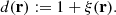
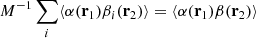
To mimic the geometry of a tomographic survey with a limited redshift coverage we selected a slab-like subset of the full simulation box. The thickness of the slab is L/5 = 300 h⁻¹ Mpc. This geometry is shown in Fig. 1. The mean number of halos in the slab is one fifth of that of the full box (156 158 objects) and varies by ±3%. For the corresponding random catalogs we generated random coordinates homogeneously inside the slab using the method +random.rand+ of the numpy python library. The number of random points in each slab is M times the number of halos, so the size of each random catalog is also slightly different.

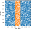Fig. 1. Geometry of the mock catalogs used in our analysis. Blue points are the full simulation box and orange points are the slab we use for our analysis. Projected here is a slice of thickness of 100 h−1 Mpc.

The area of the simulation slab corresponds to a solid angle of 1400 square degrees at z = 1, which is 9.4% of the 15 000 deg² sky coverage of the Euclid spectroscopic survey (Laureijs et al. 2011; Euclid Collaboration 2022). The thickness of the slab corresponds to a redshift bin of Δz ≈ 0.2. The mean number of objects in the slab corresponds to 5% of the survey (30 million objects). The small number of objects in the simulation made it possible to construct the sample covariance for a large number of realizations, and thus to compare the accuracy and efficiency of the LC method against that of the sample covariance.

We had 10 000 halo catalog realizations at our disposal. We divide them into two sets of 5000 realizations. We computed the sample covariance of one set, and used it as the reference covariance, against which we compared the other estimates. The reference covariance represents the best knowledge we have on the true covariance. We used the other set of 5000 realizations to compute both the LC covariance and the sample covariance, which we then compared with the reference covariance. This way we were able to estimate how much of the difference between the LC covariance and sample covariance was caused purely by the limited number of realizations.

We generated 10 000 random catalogs of size N_r = 50N_d, 5000 for the reference covariance, and 5000 for the sample covariance LC was compared with. In addition we generated 10 000 random catalogs of size N_r = 1N_d. We used a set of 5000 to serve as catalog R₁ in Eq. (24), and another set of 5000 as catalog R₂.

4.2. Random mocks

In the case of PINOCCHIO mocks we do not know the actual covariance exactly. We can only compare against the reference covariance, which itself is estimated from a finite data set. To have a test case where we know the true covariance, we ran another simulation using a purely random distribution of points as our data catalog. For this purpose we generated another set of 10 000 random mocks and used these in the place of the data catalog. Otherwise the setup was exactly the same as with PINOCCHIO mocks. We used the same slab geometry and point density, with the exception that each data catalog (and correspondingly each random catalog) realization has the same number of points: N_d = 2.3 × 10⁻⁴ (h⁻¹ Mpc)⁻³ × 6.75 × 10⁸ (h⁻¹ Mpc)³ = 155 250. The correlation function for the random distribution is zero, and for the covariance, as well as for the covariance of the covariance, an analytic result can be derived. This allowed us to directly compare the estimated covariance against the expected result.

4.3. Constructing the covariance

To validate the LC method, we computed the correlation function of the mock catalogs and constructed the LC covariance. Since we were looking for maximal reduction in the computational cost, we set M_a = 1, i.e. we used random catalogs of same size as the data catalog.

We computed the correlation function of the simulated galaxy distribution using the 2PCF code developed for the Euclid mission. The code implements the Landy-Szalay estimator with split random catalog, and stores as a by-product the DD, DR, and RR pair counts, which we need for the construction of the LC covariance. We used the Euclid code to compute the 2-dimensional correlation function $\widehat{\xi }(r,\mu )$, where r is the distance between a pair of galaxies, and μ is the cosine of the angle between the line-of-sight and the line segment connecting the galaxy pair. We used bin sizes Δr = 1 h⁻¹ Mpc and Δμ = 0.01, and computed the correlation function for the distance range r ∈ [0, 200] h⁻¹ Mpc. For some tests we needed also the 1-dimensional correlation function, which we obtained by coadding the pair counts in μ dimension. For each data catalog, we ran the code three times: once to construct the M = 50 correlation function, and twice with M = 1 random catalogs to produce the pair counts we needed for the construction of the LC covariance.

We constructed the LC and sample covariance estimates with an external code, which takes as input the precomputed pair counts. To ensure consistency, we recomputed the correlation functions from the pair counts. Having the precomputed pair counts on disk also left us the possibility of combining bins into wider ones. The run time of this external code is negligible, the CPU usage being fully dominated by the run-time of the Euclid code.

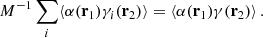
We computed the correlation function multipoles from the two-dimensional correlation function as

$$\begin{array}{c}\hfill {\xi }_{\ell }(r):=\frac{2\ell +1}{2}{\displaystyle {\int }_{-1}^1}\xi (r,\mu )P_{\ell }(\mu )\mathrm{d}\mu ,\end{array}$$(51)

where P_ℓ(μ) are Legendre polynomials (ℓ = 0, 2, 4). The M = 50 correlation function multipoles, as estimated from the simulation slabs, are depicted in Fig. 2. We show the mean over 5000 realizations, and a single realization. For this small survey size, a single realization deviates strongly from the ensemble mean, and the errors are strongly correlated between distance bins.

Fig. 2. Correlation function multipoles. Mean over 5000 PINOCCHIO realizations and a single realization. The shaded area around the single realization curve is the 1σ error envelope, computed as the standard deviation of the available realizations.

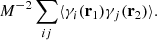
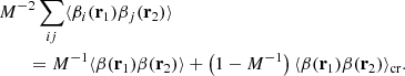
The calculation of the covariance of covariance in Sect. 3 relies on the assumption that the elements of the correlation function follow a Gaussian distribution, at least approximatively. To verify the validity of this assumption, we plot the distributions of selected correlation function elements in Fig. 3. The assumption of approximative Gaussianity seems well justified. We note that Gaussianity is only required for the covariance of covariance to be valid. The LC covariance itself does not rely on any particular distribution.

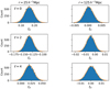Fig. 3. Histogram of correlation function multipole values at r = 25 h−1 Mpc and r = 125 h−1 Mpc. Along with the histograms we show the corresponding best-fit Gaussian distribution in orange.

5. Results

5.1. Random mocks

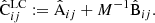
We begin by examining the one-dimensional 2PCF of the random mocks. As explained above, we ran tests using randomly distributed points in place of the data catalog. This has the benefit that we know exactly the expected correlation function (zero). We also have an accurate analytic estimate for the true covariance. From Keihänen et al. (2019) we have

$$\begin{array}{cc}& \mathrm{cov}[\widehat{\xi }({\mathbf{r}}_1),\widehat{\xi }({\mathbf{r}}_2)]\hfill \\ \hfill & =\frac{{\delta }_{12}}{G_{\mathrm{p}}({\mathbf{r}}_2)}(\frac{2}{N_{\mathrm{d}}(N_{\mathrm{d}}-1)}+\frac{4}{N_{\mathrm{d}}{N}_{\mathrm{r}}}+\frac{2}{N_{\mathrm{r}}(N_{\mathrm{d}}-1)})\hfill \\ \hfill & \approx \frac{{\delta }_{12}}{G_{\mathrm{p}}({\mathbf{r}}_1)}\frac{2}{N_{\mathrm{d}}(N_{\mathrm{d}}-1)}(1+3M^{-1}),\hfill \end{array}$$(52)

where N_r is the number of random points and N_d the number of data points, and G_p(r) is the geometrical pair volume fraction defined as

$$\begin{array}{c}\hfill G_{\mathrm{p}}(\mathbf{r})={{\displaystyle [\int {\int }_V{\mathrm{d}}^3{x}_1{\mathrm{d}}^3{x}_2]}}^{-1}{\displaystyle \int }{{\displaystyle \int }}_{V}W(x_1-x_2\in \mathbf{r}){\mathrm{d}}^3{x}_1{\mathrm{d}}^3{x}_2\end{array}$$(53)

where the integrals cover the survey volume and W(x₁ − x₂ ∈ r) = 1 if the pair distance falls in the distance bin of r, and is zero otherwise. This allows us to directly compare the estimated covariance to the theoretical one.

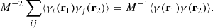
Figure 4 shows the diagonal of the estimated covariance of the one-dimensional correlation function for M = 50, compared with the theoretical value of Eq. (52). We show also the M → ∞ limit from the LC method. This represents the optimal covariance which we would have if we had an infinite random catalog. As expected, the M = ∞ curve lies slightly below the M = 50 curve. The difference is the additional uncertainty from the finite random catalog. Both the sample covariance and LC covariance agree very well with the expected covariance. It is also evident that the LC method results in larger scatter. The lower panel shows the relative difference with respect to the theoretical value, together with 1 σ error bars derived from Eqs. (31) and (38). The error for the LC covariance, measured as the standard deviation, is 2.7 times that of the sample covariance, implying that more than 7 times more realizations are needed to reach the same level of accuracy. Fortunately, from the point of view of the LC method, this is an unrealistically pessimistic situation. This can be traced to the fact that correlations, which in a more realistic situation contribute significantly to the covariance, are nonexistent here. Thus the scatter of the random catalog, which in our method is large due to the small number of objects, contributes a large fraction of the total error. The situation looks very different when we move to realistic cosmological simulations with large correlations.

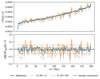Fig. 4. Diagonal covariance from random mocks, one-dimensional case. Top: sample covariance, LC, M = ∞ limit, and theoretical prediction. Bottom: the relative errors, and theoretical 1σ error estimates.

5.2. Cosmological mocks

As explained in Sect. 4.1, since we do not know the true covariance, we divided the available 10 000 realizations into two sets of 5000 realizations and used the sample covariance of the first half as a reference. We constructed the covariance for ℓ = 0, 2, 4 multipoles both through the sample covariance and with the LC method, with M = 50.

First we examine the convergence with respect to the number of realizations. This is shown in Fig. 5. We show the squared-sum difference with respect to the reference matrix, for the sample covariance and for LC. Because the bins at the smallest scales have only a few halos, we include the scales in the range 20–200 h⁻¹ Mpc in the sum. We vary the number of realizations used for the covariance estimate under study, but the reference matrix in all cases is the same, based on the full set of 5000 realizations. All matrices have been normalized to the reference diagonal, in order to assign equal weights to all distance scales,

$$\begin{array}{c}\hfill {\widehat{\mathrm{C}}}_{\mathit{ij}}(\mathrm{normalized})=\frac{{\widehat{\mathrm{C}}}_{\mathit{ij}}}{\sqrt{{\widehat{\mathrm{C}}}_{\mathit{ii}}^{\mathrm{ref}}{\widehat{\mathrm{C}}}_{\mathit{jj}}^{\mathrm{ref}}}}.\end{array}$$(54)

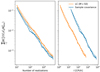Fig. 5. Convergence of the covariance of the correlation function multipoles, with respect to the number of realizations (left) and CPU time (right). We use PINOCCHIO mocks and include scales of r > 20 h−1 Mpc. Dashed lines show the theoretical prediction.

We show the difference as a function of number of realizations, and as a function of CPU time. To further reduce the noise in the measurement we compute the convergence ten times and show the mean over these ten cases. Each case is obtained by randomly splitting the 10 000 PINOCCHIO realizations into two sets of 5000 realizations, one of which used to compute the reference covariance and the other one to compute the sample and LC covariances. The different splits overlap with each other, but even so the procedure significantly reduces the noise in the measured convergence. For the same number of realizations, the sample covariance gives a smaller uncertainty. One needs roughly 1.5 times the number of realizations with LC, to reach the same level of accuracy. In terms of CPU time spent, the situation is inverted. The LC covariance requires only 10% of the CPU cost of the sample covariance to reach the same accuracy.

Of the total wall-time of constructing the sample covariance, 90% is spent on counting the pairs. In the case of LC, this fraction is somewhat lower, 76%. Loading in the catalogs takes roughly the same fraction of time in both cases so the difference in efficiency seems to be in overheads such as code initialization. A possible optimization to reduce these overheads would be to compute all the thousands of 2PCF estimates during a single code execution instead of calling the code executable over and over again.

In Fig. 6 we show the diagonal of the covariance matrix monopole block, for the sample covariance and the LC estimate, along with the reference. We show also the M = ∞ limit of the LC covariance. In the lower panel we show the relative difference with respect to the reference covariance, and the theoretical prediction for the error, as given by Eqs. (31) and (38). Since we are looking at the difference with respect to the reference, the error level shown is the square root of the sum of the variances of the reference and the estimate in question.

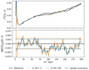Fig. 6. Diagonal of the covariance for the correlation function monopole, PINOCCHIO mocks. On the top we show the LC and sample covariance estimates, and the M = ∞ limit. On the bottom we show the relative errors, and predicted 1σ error level.

Again, the LC estimate has more internal scatter than the sample covariance, but the difference between the methods is significantly smaller than in the case of random mocks. A more striking phenomenon is that the deviation from the reference is strongly correlated in distance, and the general trend of the deviation is very similar for the two estimation methods. In other words, the estimation error is dominated by a correlated error component that is independent of the chosen estimation method, when both estimates are constructed from the same data set. The common component dominates over the additional noise added by the LC method. The amplitude of the component is consistent with the predicted error level, indicating that it represents a random fluctuation.

Figure 7 shows the monopole block of the full LC covariance matrix as a two-dimensional plot. For plotting purposes we normalize the matrix by the diagonal of the reference covariance. There is significant off-diagonal component, showing that the error in the estimated Landy–Szalay correlation function is correlated from one distance bin to another, in line with Fig. 6. The middle panel shows the difference between the LC covariance and the reference. There is no obvious overall bias (which would show up as the over-representation of either the blue or the red color), but the region of correlated error is clearly visible around 100 h⁻¹ Mpc. The bottom panel shows the difference between the LC and sample covariances from the same 5000 realizations. Here the structure is weaker, indicating that the correlated structure in the middle panel is for a large part common for the sample covariance and the LC estimate, as we already saw in Fig. 6.

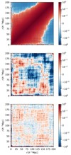Fig. 7. Monopole block of the covariance matrix. Top: LC covariance matrix. Middle: difference between the LC covariance matrix and the reference. Bottom: difference between the LC and the sample covariance from same realizations. All are normalized by the diagonal elements of the reference matrix.

We proceed to examine the structure of the LC covariance further. We show the $\widehat{\text{A}}$ and $\widehat{\text{B}}$ components for the full multipole covariance in Fig. 8, again normalized with the reference diagonal. The full covariance will be the combination $\widehat{\text{A}}+\widehat{\text{B}}/M$. We observe that the $\widehat{\text{B}}$ component is strongly diagonal-dominated, in contrast to the $\widehat{\text{A}}$ component, indicating that the finite random catalog mainly contributes uncorrelated noise to the 2PCF estimate, on top of the correlated error that arises from the data catalog. The unnormalized diagonals of all three multipole blocks, and their cross-components, are shown in Fig. 9.

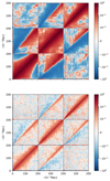Fig. 8. Component matrices $\widehat{\text{A}}$ (top) and $\widehat{\text{B}}$ (bottom), for correlation function multipoles, measured from the PINOCCHIO mocks. The blocks from left to right and from the bottom to the top row correspond to ℓ = 0, 2, 4 multipoles, respectively. Both are normalized by the diagonal elements of the reference matrix.

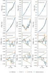Fig. 9. Covariance diagonals for multipoles ℓ = 0, 2, 4, and their cross-correlation, for PINOCCHIO. Sample covariance and LC. Two bottom rows show the difference between the reference and the estimate scaled by r2. To reduce scatter in the curves all the quantities have been rebinned to bins of width of 10 h−1 Mpc.

The expectation value of the LC covariance in terms of pair-count covariances is given in Eq. (21). However, if we expand Eq. (26) (which defines the LC covariance) in terms of pair-count covariances, we find that the expansion includes more terms than Eq. (21). The expectation value of these additional terms vanishes, but when the covariance is estimated from a finite number of correlation function realizations, these terms differ from zero randomly. This raises the question whether leaving some or all of these zero-expectation-value terms out and constructing the covariance using the pair-count covariances directly would reduce noise in the covariance matrix estimate. We reconstructed the covariance matrix by including all the possible combinations of the zero-expectation-value terms, but it turned out that the most accurate combination is the one defined by Eq. (26). Even though the pair-count covariances do not affect the expectation value of the covariance matrix estimate, they do reduce its variance. This can be understood as follows: the zero-expectation terms are negatively correlated with some of the nonzero terms, and thus they help to cancel out part of the estimation noise.

5.3. Predictions from covariance of covariance

We now proceed to examine the accuracy of the LC covariance estimate in a more quantitative way. Here we make use of predictions of the theoretical covariance of covariance from Sect. 3.

We measure the accuracy of the covariance estimate, as the normalized sum-of-squares difference from the ensemble-average, over all covariance elements,

$$\begin{array}{c}\hfill {\chi }_N^2:=\frac{1}{N_{\mathrm{bin}}^2}{\displaystyle \sum _{\mathit{ij}}\frac{1}{{\widehat{\mathrm{C}}}_{\mathit{ii}}^{\mathrm{ref}}{\widehat{\mathrm{C}}}_{\mathit{jj}}^{\mathrm{ref}}}{({\widehat{\mathrm{C}}}_{\mathit{ij}}-⟨{\mathrm{C}}_{\mathit{ij}}⟩)}^2.}\end{array}$$(55)

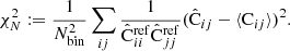
Here $\widehat{\text{C}}$ represents the covariance estimate, either LC or sample covariance, measured from N realizations (5000), and N_bin is the number of correlation function elements. In our baseline simulation N_bin = 540 (3 multipoles and 180 distance bins). We normalized the sum by the diagonal of the reference covariance, to assign equal weights to all distance bins. Equation (55) expresses the accuracy of the covariance as a single number.

In terms of the covariance of covariance we have

$$\begin{array}{c}\hfill ⟨{\chi }_N^2⟩=\frac{1}{N_{\mathrm{bin}}^2}{\displaystyle \sum _{\mathit{ij}}}\frac{\mathrm{cov}({\widehat{\mathrm{C}}}_{\mathit{ij}},{\widehat{\mathrm{C}}}_{\mathit{ij}})}{{\widehat{\mathrm{C}}}_{\mathit{ii}}^{\mathrm{ref}}{\widehat{\mathrm{C}}}_{\mathit{jj}}^{\mathrm{ref}}}.\end{array}$$(56)

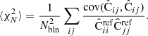
Since the covariance of covariance scales as 1/(N − 1), we can write this in terms of the N = 2 value as

$$\begin{array}{c}\hfill ⟨{\chi }_N^2⟩=\frac{⟨{\chi }_2^2⟩}{N-1}.\end{array}$$(57)

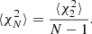
For the sample covariance we now have

$$\begin{array}{c}\hfill {⟨{\chi }_2^2⟩}^{\mathrm{Smp}}=\frac{1}{N_{\mathrm{bin}}^2}{\displaystyle \sum _{\mathit{ij}}({\stackrel{\sim }{\mathrm{C}}}_{\mathit{ii}}{\stackrel{\sim }{\mathrm{C}}}_{\mathit{jj}}+{\stackrel{\sim }{\mathrm{C}}}_{\mathit{ij}}^2),}\end{array}$$(58)

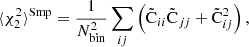
where we have absorbed the normalization into the covariance, and denoted the normalized covariance by $\stackrel{\sim }{\text{C}}$. For LC we find

$$\begin{array}{cc}\hfill {⟨{\chi }_2^2⟩}^{\mathrm{LC}}& =\frac{1}{N_{\mathrm{bin}}^2}{\displaystyle \sum _{\mathit{ij}}}[{\stackrel{\sim }{\mathrm{D}}}_{\mathit{ii}}{\stackrel{\sim }{\mathrm{D}}}_{\mathit{jj}}+{\stackrel{\sim }{\mathrm{D}}}_{\mathit{ij}}^2\hfill \\ \hfill & +{(\frac{1}{2}-M^{-1})}^2({\stackrel{\sim }{\mathrm{B}}}_{\mathit{ii}}{\stackrel{\sim }{\mathrm{B}}}_{\mathit{jj}}+{\stackrel{\sim }{\mathrm{B}}}_{\mathit{ij}}^2)].\hfill \end{array}$$(59)

Here we have a practical way of predicting the estimation error for the LC and sample covariance, for different values of M. We can also easily predict the effect of rebinning the data into wider distance bins, simply by rebinning the covariance matrices and constructing the covariance of covariance from these.

In Table 3 we have collected statistics on the estimation methods, for a selected random catalog size (different values of M) and for different rebinning schemes. We have used $\widehat{\text{A}}$ and $\widehat{\text{B}}$ in the place of A and B, and 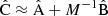$\widehat{\text{C}}\approx \widehat{\text{A}}+M^{-1}\widehat{\text{B}}$ in the place of C. We show the computational cost of pair counting in each of the cases, in the units of counting the pairs in one N_d data catalog. The cost of the LC method is the same in all cases, while the cost of the sample covariance scales as 1 + 3M. The cost estimate ignores parts of the computation other than pair counting, for instance disk I/O and various overheads, thus exaggerating the difference between the methods. The estimator variance is expressed as ${\chi }_2^2$. The standard deviation of a covariance estimate is obtained from this as $\sqrt{{\chi }_2^2/(N-1)}$. We show also an inverse figure-of-merit (iFoM) constructed as the product of the pair-count cost and the ${\chi }_2^2$ value. Since the estimator variance decreases proportionally to the inverse of the number of realizations N, while the computation time grows proportional to it, this is an N-independent measure of the estimator efficiency. A smaller value indicates a more efficient estimation. The value of iFoM can be interpreted as the computational cost of reaching ${\chi }_2^2$ = 1. The last column shows the ratio of the sample-covariance iFoM to that of the LC covariance, and is measure of the gain from the LC method.

The relative efficiency of the LC method increases with increasing M, as the computational cost of the sample covariance becomes larger. We observe also that for given M, the LC covariance becomes more efficient in comparison to sample covariance, if we combine the distance bins into wider bins. With M = 50 and with 20 h⁻¹ Mpc bins in distance, the efficiency ratio is 17.9, while with narrow 1 h⁻¹ Mpc bins the ratio is 11.9.

The full covariance of covariance is a four-dimensional data object, and is difficult to visualize in its entirety. In the following we examine a two-dimensional subset. We focus on the diagonal of the monopole block of the covariance estimate (plotted in Fig. 6). This is a 1-dimensional data object, thus its covariance is a 2-dimensional matrix. In the following we refer to the covariance of the diagonal of the monopole block of a 2PCF covariance estimate as COVCOV for short. We plot the predicted COVCOV for the sample covariance and for LC in Fig. 10. In both cases, there is a significant off-diagonal structure, which is visually very similar between the two methods. This verifies our earlier observation that the estimation error is correlated between distance bins, and this correlation does not depend on the chosen method. Taking the difference between the COVCOV matrices, we see that the LC estimate has additional scatter compared to the sample covariance, but this additional error component is only weakly correlated from one distance bin to another.

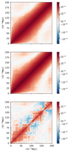Fig. 10. Predicted covariance of the diagonal of the monopole block of the estimated 2PCF covariance (COVCOV). Top: COVCOV for sample covariance. Middle: COVCOV for LC. Bottom: difference of the two. From normalized covariances.

As a final validation test we applied the inverse square root of the COVCOV to the difference between the LC covariance matrix diagonal and the corresponding reference (quantities plotted in Fig. 6). If the COVCOV correctly describes the errors in the estimated covariance, we expect to see an array of white noise with σ = 1. To account for the fact that the reference covariance has a covariance of its own, we took the COVCOV to be the sum of the reference and the LC COVCOV matrices. We computed the square root using the Schur method implemented in the +scipy+ Python library. The resulting whitened data vector is shown in Fig. 11, along with a random realization of white noise. The data is visually indistinguishable from white noise, which is a valuable validation check. The similarity can also be confirmed by computing a normalized χ² value

$$\begin{array}{c}\hfill {\chi }^2=\frac{1}{N}{\mathbf{v}}^{\mathrm{T}}\mathbf{v}.\end{array}$$(60)

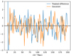Fig. 11. Diagonal monopole difference treated with the inverse square root of COVCOV. For reference a Gaussian random vector of same length.

Here v is the data vector, N is the number of bins, and for a vector of Gaussian white noise we expect a value close to 1. We computed this value for scales r > 20 h⁻¹ Mpc and obtained χ² = 0.95 for the whitened data vector and χ² = 0.93 for the Gaussian random vector.

6. Conclusions

We have presented a method for speeding up the computation of the galaxy 2PCF covariance. We have named the method as the Linear Construction, or LC method. We assume that the correlation function is estimated through Landy–Szalay estimator, with a split random catalog. The proposed method applies both to the raw (1- or 2-dimensional) correlation function and to its multipoles.

The proposed method provides an unbiased estimate of the covariance for a split random catalog, that is, for a case where the random-random pair count is constructed as the coadded sum of many small subcatalogs. Since we know that the splitting only weakly affects the 2PCF estimation error, we expect that the LC covariance provides a good approximation also when the RR pairs are counted from the full catalog. This can be traced to the fact that, for large random catalogs, the 2PCF estimation error is dominated by the variance of the galaxy sample, and the secondary error term is related to the data-random pair count, both of which are unaffected by splitting. The scatter of the random-random count plays a minor role.

The computational cost of the LC method per realization, for a random catalog M times the size of the data catalog, is a factor of (1 + 3M)/7 lower than that of the sample covariance. For M = 50 this yields a factor of 21.6 speedup. However, a larger number of realizations is needed, to compensate for the increased scatter in the estimate. In our simulations, 1.2–1.8 times higher a number of realizations was needed to reach a given level of accuracy, depending on bin size. This taken into account, the net cost reduction for M = 50 is a factor of 11.9–17.9. The efficiency increases with increasing bin width. In practice, we observe a halved speedup due to the heavy overhead associated with the handling of many small catalogs. A code specially optimized for covariance computation could improve on this.

The computational cost of the LC covariance is independent of M. Thus the relative gain with respect to the sample covariance increases with increasing size of the random catalog. Since the cost of the covariance computation exceeds that of the actual 2PCF estimation by orders of magnitude, one might want to spend a bit more resources on obtaining a more accurate 2PCF estimate with a higher M, as the cost of the covariance is unaffected.

The LC covariance estimate is readily extrapolated to an arbitrary value of M, including the limit M → ∞. We thus have an estimate of the error budget for any number of random points. which is valuable information when planning for an experiment.

At very small distances our method becomes less reliable due to the small number of objects in a bin. At those small distances we recommend resorting to sample covariance, which at small distances is cheap anyway.

Unlike the sample covariance, the LC covariance is not by construction positive-definite. For applications that require the covariance inverse, we recommend verifying the eigenspectrum of the constructed matrix, and for instance rebinning the data to wider bins, should the matrix turn out to be nonpositive definite.

We further derived a covariance for the estimation error of the LC covariance, and showed that it can be constructed from the components of the covariance itself. Thus, along with the covariance one can readily obtain an estimate of its errors and their correlation. We also discussed the impact on maximum-likelihood parameter estimation.

In the LC method, the covariance is estimated for small random catalogs of size M = M_a and M = 2M_a, and the covariance for arbitrary M is constructed as a linear combination of these. We obtain the maximal reduction in the computational cost with M_a = 1, and we adopted this value in our validation tests. The increased uncertainty in the covariance estimate is compensated for with a larger number of catalog realizations. We have assumed that the mock catalogs are cheap to generate, so that they do not significantly contribute to the total CPU budget. Should this not be the case, the gain from the LC covariance is reduced in comparison with the sample covariance. In this case it may become beneficial to select M_a > 1, to reduce the variance of the covariance estimate. The selection of the optimal method is a trade-off between the cost of the 2PCF computation, the required level of accuracy, and the cost of constructing the mock catalogs.

Future large galaxy surveys, such as the one provided by Euclid, face the challenge of constructing the covariance for huge galaxy samples. We believe the methodology presented here provides a useful tool for meeting that challenge.

Acknowledgments

The 2PCF computations were done at the Euclid Science Data Center Finland (SDC-FI, urn:nbn:fi:research-infras-2016072529), for whose computational resources we thank CSC – IT Center for Science, the Finnish Grid and Cloud Computing Infrastructure (FGCI, urn:nbn:fi:research-infras-2016072533), and the Academy of Finland grant 292882. This work was supported by the Academy of Finland grant 295113. The Euclid Consortium acknowledges the European Space Agency and a number of agencies and institutes that have supported the development of Euclid, in particular the Academy of Finland, the Agenzia Spaziale Italiana, the Belgian Science Policy, the Canadian Euclid Consortium, the French Centre National d’Etudes Spatiales, the Deutsches Zentrum für Luft- und Raumfahrt, the Danish Space Research Institute, the Fundação para a Ciência e a Tecnologia, the Ministerio de Economia y Competitividad, the National Aeronautics and Space Administration, the National Astronomical Observatory of Japan, the Netherlandse Onderzoekschool Voor Astronomie, the Norwegian Space Agency, the Romanian Space Agency, the State Secretariat for Education, Research and Innovation (SERI) at the Swiss Space Office (SSO), and the United Kingdom Space Agency. A complete and detailed list is available on the Euclid web site (http://www.euclid-ec.org).

References

All Tables

All Figures

	Fig. 1. Geometry of the mock catalogs used in our analysis. Blue points are the full simulation box and orange points are the slab we use for our analysis. Projected here is a slice of thickness of 100 h−1 Mpc.
In the text

	Fig. 2. Correlation function multipoles. Mean over 5000 PINOCCHIO realizations and a single realization. The shaded area around the single realization curve is the 1σ error envelope, computed as the standard deviation of the available realizations.
In the text

	Fig. 3. Histogram of correlation function multipole values at r = 25 h−1 Mpc and r = 125 h−1 Mpc. Along with the histograms we show the corresponding best-fit Gaussian distribution in orange.
In the text

	Fig. 4. Diagonal covariance from random mocks, one-dimensional case. Top: sample covariance, LC, M = ∞ limit, and theoretical prediction. Bottom: the relative errors, and theoretical 1σ error estimates.
In the text

References

- Akeson, R., Armus, L., Bachelet, E., et al. 2019, ArXiv e-prints [arXiv:1902.05569] [Google Scholar]
- Alam, S., Ata, M., Bailey, S., Beutler, F., et al. 2005, MNRAS, 470, 2617 [Google Scholar]
- Alam, S., Aubert, M., Avila, S., et al. 2021, Phys. Rev. D, 103, 083533 [NASA ADS] [CrossRef] [Google Scholar]
- Anderson, T. W. 2003, An Introduction to Multivariate Statistical Analysis (Wiley Interscience), 3rd ed. [Google Scholar]
- Colavincenzo, M., Sefusatti, E., Monaco, P., et al. 2019, MNRAS, 482, 4883 [NASA ADS] [CrossRef] [Google Scholar]
- Cole, S., Percival, W., Peacock, J., et al. 2005, MNRAS, 362, 505 [NASA ADS] [CrossRef] [Google Scholar]
- Dávila-Kurbán, F., Sánchez, A. G., Lares, M., & Ruiz, A. N. 2021, MNRAS, 506, 4667 [CrossRef] [Google Scholar]
- DESI Collaboration (Aghamousa, A., et al.) 2016, ArXiv e-prints [arXiv:1611.00036] [Google Scholar]
- Dodelson, S., & Schneider, D. 2013, Phys. Rev. D, 88, 063537 [NASA ADS] [CrossRef] [Google Scholar]
- Eisenstein, D. J., Zehavi, I., Hogg, D. W., et al. 2005, ApJ, 633, 560 [Google Scholar]
- Euclid Collaboration (Scaramella, R., et al.) 2022, A&A, 662, A112 [NASA ADS] [CrossRef] [EDP Sciences] [Google Scholar]
- Friedrich, O., & Eifler, T. 2018, MNRAS, 473, 4150 [NASA ADS] [CrossRef] [Google Scholar]
- Gaztañaga, E., & Scoccimarro, R. 2005, MNRAS, 361, 824 [Google Scholar]
- Hartlap, J., Simon, P., & Schneider, P. 2007, A&A, 464, 399 [NASA ADS] [CrossRef] [EDP Sciences] [Google Scholar]
- Ivezić, Ž., Kahn, S. M., Tyson, J. A., et al. 2019, ApJ, 873, 111 [Google Scholar]
- Jasche, J., & Lavaux, G. 2017, A&A, 606, A37 [NASA ADS] [CrossRef] [EDP Sciences] [Google Scholar]
- Joachimi, B. 2017, MNRAS, 466, L83 [NASA ADS] [CrossRef] [Google Scholar]
- Kalus, B., Percival, W. J., Bacon, D. J., et al. 2019, MNRAS, 482, 453 [CrossRef] [Google Scholar]
- Keihänen, E., Kurki-Suonio, H., Lindholm, V., et al. 2019, A&A, 631, A73 [NASA ADS] [CrossRef] [EDP Sciences] [Google Scholar]
- Kitaura, F.-S., Rodríguez-Torres, S., Chuang, C.-H., et al. 2016, MNRAS, 456, 4156 [NASA ADS] [CrossRef] [Google Scholar]
- Landy, S. D., & Szalay, A. S. 1993, ApJ, 412, 64 [Google Scholar]
- Laureijs, R., Amiaux, J., Arduini, S., et al. 2011, ArXiv e-prints [arXiv:1110.3193] [Google Scholar]
- Manera, M., Scoccimarro, R., Percival, W. J., et al. 2013, MNRAS, 428, 1036 [Google Scholar]
- Merz, G., Rezaie, M., Seo, H.-J., et al. 2021, MNRAS, 506, 2503 [NASA ADS] [CrossRef] [Google Scholar]
- Monaco, P. 2016, Galaxies, 4, 53 [NASA ADS] [CrossRef] [Google Scholar]
- Monaco, P., Theuns, T., & Taffoni, G. 2002, MNRAS, 331, 587 [Google Scholar]
- Monaco, P., Di Dio, E., & Sefusatti, E. 2019, JCAP, 2019, 023 [CrossRef] [Google Scholar]
- Munari, E., Monaco, P., Sefusatti, E., et al. 2017, MNRAS, 465, 4658 [Google Scholar]
- Padmanabhan, N., White, M., Zhou, H. H., & O’Connell, R. 2016, MNRAS, 460, 1567 [NASA ADS] [CrossRef] [Google Scholar]
- Paz, D. J., & Sánchez, A. G. 2015, MNRAS, 454, 4326 [NASA ADS] [CrossRef] [Google Scholar]
- Percival, W. J., Ross, A. J., Sánchez, A. G., et al. 2014, MNRAS, 439, 2531 [NASA ADS] [CrossRef] [Google Scholar]
- Percival, W. J., Friedrich, O., Sellentin, E., & Heavens, A. 2022, MNRAS, 510, 3207 [NASA ADS] [CrossRef] [Google Scholar]
- Pope, A. C., & Szapudi, I. 2008, MNRAS, 389, 766 [NASA ADS] [CrossRef] [Google Scholar]
- Sellentin, E., & Heavens, A. F. 2016, MNRAS, 456, L132 [Google Scholar]
- Taylor, A., & Joachimi, B. 2014, MNRAS, 442, 2728 [Google Scholar]
- Taylor, A., Joachimi, B., & Kitching, T. 2013, MNRAS, 432, 1928 [Google Scholar]
All Tables
Predictions for the variance of the covariance estimate, based on the covariance of covariance for PINOCCHIO mocks.