| Issue |
A&A
Volume 652, August 2021
|
|
|---|---|---|
| Article Number | A121 | |
| Number of page(s) | 10 | |
| Section | Planets and planetary systems | |
| DOI | https://doi.org/10.1051/0004-6361/202140529 | |
| Published online | 18 August 2021 | |
High-contrast imaging at ten microns: A search for exoplanets around Eps Indi A, Eps Eri, Tau Ceti, Sirius A, and Sirius B
1
European Southern Observatory,
Karl-Schwarzschild-Str. 2,
85748
Garching bei München,
Germany
e-mail: This email address is being protected from spambots. You need JavaScript enabled to view it.
2
Space sciences, Technologies and Astrophysics Research (STAR) Institute, Université de Liège,
19c Allée du Six Août,
4000
Liège,
Belgium
3
Institut für Teilchen- und Astrophysik ETH Zurich,
Switzerland
4
Center for Astronomy Research, University of Hertfordshire,
Hatfield,
UK
5
Stockholm University, Stockholm Observatory,
Sweden
6
AIM, CEA, CNRS, Université Paris-Saclay, Université Paris Diderot,
Sorbonne Paris Cité,
91191
Gif-sur-Yvette,
France
7
Astronomy Department, University of Michigan,
Ann Arbor,
MI
48109,
USA
8
Tsung-Dao Lee Institute, Shanghai Jiao Tong University,
800 Dongchuan Road,
Shanghai
200240,
PR China
9
Department of Astronomy, School of Physics and Astronomy, Shanghai Jiao Tong University,
800 Dongchuan Road,
Shanghai
200240,
PR China
Received:
10
February
2021
Accepted:
26
April
2021
Abstract
Context. The direct imaging of rocky exoplanets is one of the major science goals of upcoming large telescopes. The contrast requirement for imaging such planets is challenging. However, the mid-IR (infrared) regime provides the optimum contrast to directly detect the thermal signatures of exoplanets in our solar neighbourhood.
Aims. We aim to exploit novel fast-chopping techniques newly developed for astronomy with the aid of adaptive optics to look for thermal signatures of exoplanets around bright stars in the solar neighbourhood.
Methods. We used the upgraded Very Large Telescope Imager and Spectrometer for the mid-InfraRed (VISIR) instrument with high-contrast imaging capability optimised for observations at 10 μm to look for exoplanets around five nearby (d < 4 pc) stars. The instrument provides an improved signal-to-noise ratio (S/N) by a factor of ~4 in the N-band compared to standard VISIR for a given S/N and time.
Results. In this work, we achieve a detection sensitivity of sub-mJy, which is sufficient to detect a few Jupiter mass planets in nearby systems. Although no detections are made, we achieve most sensitive limits within <2″ for all the observed targets compared to previous campaigns. For ϵ Indi A and ϵ Eri, we achieve detection limits very close to the giant planets discovered by RV, with the limits on ϵ Indi A being the most sensitive to date. Our non-detection therefore supports an older age for ϵ Indi A. The results presented here are promising for high-contrast imaging and exoplanet detections in the mid-IR regime.
Key words: planets and satellites: detection / instrumentation: adaptive optics
F.R.S.-FNRS Research Associate.
© ESO 2021
1 Introduction
The direct imaging of habitable exoplanets is one of the key science goals of current and upcoming large telescopes (Meyer et al. 2018). The field of high-contrast imaging (HCI), employing extreme adaptive optics (ExAO), coronagraphy, and state-of-the-art post-processing techniques, has enabled the direct imaging of young (up to about 30 Myr), several-Jupiter-mass exoplanets with current 8–10 m class telescopes (Marois et al. 2008; Macintosh et al. 2015; Keppler et al. 2018; Chauvin et al. 2017; Nowak et al. 2020). Examples of current HCI instruments include the Spectro-Polarimetric High-contrast Exoplanet REsearch instrument (SPHERE), the Gemini Planet Imager (GPI), and Subaru Coronagraphic Extreme Adaptive Optics (SCExAO), all of which operate in the near-IR (1–2.5 μm) regime (Beuzit et al. 2019; Macintosh et al. 2014; Jovanovic et al. 2015). Compared to the near-IR, the mid-IR (8–13 μm) is more sensitive to colder planets and allows to probe less massive planets or, for a given mass, one is able to search around older stars (Quanz et al. 2015). This is because the planet-to-star flux contrast is more favourable in the mid-IR, where the thermal emission of the planet peaks in the Rayleigh–Jeans tail of target stars (Baraffe et al. 2003; Sudarsky et al. 2003; Marley et al. 2007; Fortney et al. 2008; Spiegel & Burrows 2012). The key downsides of mid-IR HCI are reduced spatial resolution due to the larger diffraction limit and large sky background for ground-based observations. Therefore, the mid-IR is best suited to looking for exoplanets around nearby stars.
New Earths in the α Cen Region (NEAR) experiment was a collaboration between the Breakthrough Foundation and the European Southern Observatory(ESO). The project involved upgrading the existing VISIR (Very Large Telescope Imager and Spectrometer for the mid-InfraRed) instrument (Lagage et al. 2004) at the VLT with adaptive optics (AO) using the deformable secondary mirror (DSM) installed at UT4 (Arsenault et al. 2017), and a high-performance annular groove phase mask (AGPM) coronagraph (Mawet et al. 2005). The aim of the NEAR experiment was to enable HCI capability in the astronomical N-band and to look for low mass exoplanets in the α Centauri binary system in a 100 h campaign (for details, see Kasper et al. 2017, 2019). The NEAR was able to reach sensitivity and contrast sufficient for the detection of Neptune-mass planets in the habitable zone of α Cen A, and a weak signal was found, the nature of which (e.g. planet, part of a zodiacal disc, image artefact) remains to be confirmed by follow-upobservations (for details, see Wagner et al. 2021).
In this work, we report the results of observations with NEAR to look for Jupiter-sized exoplanets around the nearest stars with spectral types earlier than M: ϵ Indi A, ϵ Eri, τ Ceti, Sirius A, and Sirius B. In Sect. 2, we briefly describe observed targets; in Sects. 3 and 4, we describe the data observation and reduction techniques. We discuss results in Sect. 5 and conclude with Sect. 6.
2 Target description
2.1 ϵ Indi A
ϵ Indi is a triple system at a distance of 3.6 pc (Gaia Collaboration 2021). It consists of the primary K5V star ϵ Indi A and a brown dwarf binary (ϵ Indi Ba and Bb) on a wide orbit of 1459 AU (Scholz et al. 2003; McCaughrean et al. 2004). Age estimates of  Gyr for ϵ Indi A were published based on chromospheric activity indicators such as the calcium RHK as a proxy for rotation (Lachaume et al. 1999). Given the well-known relationships between rotation and age for FGK stars a similar value of 1.5 Gyr was suggested by Kasper et al. (2009). However, Dieterich et al. (2018) suggested an older age based on UVW kinematics and cooling curves for the brown dwarf companions. Recently, Feng et al. (2019) used extensive time-resolved spectra to estimate a rotation period for the star of 36 days, suggesting an age of ~ 4 Gyr based on the rotation-age calibration of Eker et al. (2015). This older age also agrees with the 3.7–4.3 Gyr estimated by King et al. (2010) for the brown dwarf binary from the dynamical system mass and the evolutionary models of Baraffe et al. (2003). The higher end of the age range is therefore more likely.
Endl et al. (2002) first identified a long-period, low-amplitude radial velocity signal in ϵ Indi A, which could be explained by a companion with P > 20 yr and a mass of at least 1.6 MJ . This signal was confirmed by Janson et al. (2009) and Zechmeister et al. (2013), who also found that the binary brown dwarf companions ϵ Indi Ba and Bb are too far away to induce the measured trend. Feng et al. (2019) combine radial velocity data with astrometry to confirm the existence of a  ,MJ planet on an eccentric orbit with a period of
  yr. In September 2019, at the time of our observations, the separation of this planet from the host star is expected to be about 1.07′′ (error bars are large due to poorly constrained orbital solution).
2.2 ϵ Eri
ϵ Eri is an adolescent K2V type dwarf star at a distance of 3.2 pc (Gaia Collaboration 2021). The age of the star has been estimated through various means and is generally thought to be around 0.4–0.9 Gyr, with the higher end of the range being more likely (Henry et al. 1996; Song et al. 2000; Di Folco et al. 2004; Mamajek & Hillenbrand 2008). ϵ Eri is surrounded by a narrow ring of debris located between 63 and 76 AU and a possible inner belt from 12 to 16 AU (see Mawet et al. 2019, for a full discussion of the disc structure).
A companion to ϵ Eri was first suggested by Walker et al. (1995) based on radial velocity data. Hatzes et al. (2000) argued that the most likely explanation for the observed decade-long radial velocity (RV) variations was the presence of a 1.5 MJ giant planet with a period P = 6.9 yr (3 AU orbit) and a high eccentricity (e = 0.6). Very similar parameters for the planet ϵ Eri b were derived from a comprehensive set of RV as well HST astrometry data by Benedict et al. (2006). The most recent mass estimate to date was done by Mawet et al. (2019) and combined 30 yr of radial velocity data with deep direct imaging data in a Bayesian analysis to constrain the properties of the companion. They found a mass of  , MJ at a separation of 3.48 ± 0.07 AU and an eccentricity of 0.007, which is lower than previously reported values. Direct imaging detections of ϵ Eri b in the L- and M-bands were attempted by Janson et al. (2008) and Mawet et al. (2019) and yielded upper mass limits of around 4 MJ (for an age of 320 Myr) and 2 MJ (for 400 Myr), respectively. A second companion was first suggested by Benedict et al. (2006) at 12–20 AU based on radial velocity residuals, but this was not confirmed by Mawet et al. (2019). An alternative additional companion of 0.4–1.2 MJ has been suggested at 48 AU by Booth et al. (2017) to explain the shape of the outer dust belt, and Mawet et al. (2019) also required an additional planet to stir this belt. Janson et al. (2015) are able to obtain sub-Jovian mass limits of 0.6–1 MJ at these larger separations, but this cannot rule out the lower end of the proposed mass range, so while the companion has not been confirmed, it can also not been ruled out.
2.3 τ Ceti
τ Ceti is a nearby (3.7 pc), sun-like G8.5V star with an extended debris disc (5–55 AU) that is more than ten times as massive as the Kuiper belt (Gaia Collaboration 2021; Gray et al. 2006; Greaves et al. 2004; MacGregor et al. 2016). There is a large range in the literature for ages of τ Ceti: based on stellar activity the age is 5.8 ± 2.9 Gyr (Mamajek & Hillenbrand 2008), but astroseismological and interferometric measurements suggest an age closer to 8–10 Gyr (Di Folco et al. 2004; Tang & Gai 2011) and chemical composition measurements point towards an age of  Gyr (Pagano et al. 2015).
Tuomi et al. (2013) discovered five Earth-like planets in radial velocity data with periods from 14 to 642 days (0.1–1.35 AU). Two of these were confirmed by Feng et al. (2017), who discovered two further planets at periods of 20 and 49 days. They also suggest that the 14-day signal could be the result of stellar activity rather than a planet, and that candidates e, f, and h might actually be too eccentric to be planets. Dietrich & Apai (2021) used dynamical arguments to provide statistical evidence for the existence of the remaining three planets suggested by Tuomi et al. (2013) and one additional candidate that could be located in the habitable zone. All the previously mentioned candidates are expected to be super-Earths (M ⋅ sin(i) ≈ 1–4 M⊕). However, Kervella et al. (2019) provided tentative evidence of a giant planet candidate (1–2 MJ , 3–20 AU) from Gaia data. Near-IR direct imaging has not been able to detect any of the planets, but has provided constraints of 10–20 MJ at separations larger than 2′′ (7AU) and 30–50 MJ at 1′′ (Boehle et al. 2019). The candidate detected by Kervella et al. (2019) is the only one that is not too small and close to the host star to be detected with present-day mid-IR facilities.
Observing parameters for all the targets under various conditions.
2.4 Sirius A
Sirius is a binary system at a distance of 2.7 pc, consisting of an A1Vm star and a WD with an age of 225–250 Myr (Gaia Collaboration 2021; Liebert et al. 2005; Bond et al. 2017). While there are no known planets around Sirius A or B, there are mass limits on possible companions from previous imaging campaigns covering wavelengths of roughly 0.5–5 μm. The most sensitive limits on Sirius A exclude giant planets down to 11 MJ at 0.5 AU, 6–7 MJ in the 1–2 AU range and 4 MJ at 10 AU (Hunziker et al. 2020; Vigan et al. 2015; Thalmann et al. 2011; Bonnet-Bidaud & Pantin 2008). In any case, the long-term orbital stability of planets around Sirius A or B would be impacted by the binarity of the system, which has a semi-major axis of about 20 AU and eccentricity 0.6. Bond et al. (2017) find that the longest periods for stable planetary orbits in the Sirius system are about 2.24 yr for a planet orbiting Sirius A, corresponding to a r = 2.2 AU circular orbit, and 1.79 yr for a planet orbiting Sirius B, corresponding to a r = 1.5 AU circular orbit. WDs are typically 103 to 104 times less luminous than their progenitor stars. Thus, it would be much easier to achieve the contrast required to detect a planetary companion (Burleigh et al. 2002). This idea sparked direct imaging searches for planets around WDs (Gratton et al. 2021; Friedrich et al. 2007). While no planets have been found using direct imaging to date, a transiting planet was found around the white dwarf WD 1856+534 (Vanderburg et al. 2020), and an evaporating Neptune was proposed to explain the chemical fingerprints of hydrogen, oxygen, and sulfur in the spectrum of WDJ0914+1914 (Gänsicke et al. 2019).
2.5 Sirius B
For Sirius B, as explained above a planet in a stable orbit would have a period of 1.79 yr when r = 1.5 AU. No limits have been placed on companions within 3′′, although near-IR imaging by Bonnet-Bidaud & Pantin (2008) did set limits of 10–30 MJ outside of that radius. Sirius B is the only target in the sample to have been previously imaged in the mid-IR at 8–10 μm between 2003 and 2006, but no limits on companions were determined from this dataset (Skemer & Close 2011).
3 Observation and data reduction
3.1 Observation
All the observations employed a common observing strategy, including the use of AO, an AGPM coronagraph, chopping, and nodding. The chopping was done with the DSM of the VLT. The chop throw of the DSM was 4.5″ and was performed at a speed of 8.33 Hz to reduce the excess low-frequency noise common to the mid-IR arrays (Si:As array, Arrington et al. 1998). The chopping subtracts two images taken at different positions on the sky, thereby leaving a positive (coronagraphic, on-axis) and a negative (off-axis) image of the source separated by the chop throw and removing most of the sky and instrumental background flux bias. However, the optical path is slightly different for both chopping positions, which leaves some small residuals. In principle, these could be removed by nodding (for details see Lagage et al. 2004), but our data reduction is not affected by the small chopping residuals which are not point-like and do not degrade the point-source sensitivity. At 8.33 Hz chopping, each half-cycle is 60 ms consisting of 8 × 6 ms DITs (= 48 ms) and 2 × 6 ms DITs (= 12 ms) skipped during the chopping transition. The other half-cycle is taken with the star off the coronagraph. At each nodding position, 500 chopping frames’ half-cycles were recorded for a total observing time of 500 × 60 ms = 30 s, out of which 250 × 48 ms = 12 were spent with the target on the coronagraph, that is, the observing efficiency was 40%. A summary of the observations and the atmospheric conditions affecting the sensitivity is outlined in Table 1. The atmospheric data were taken from the Paranal astronomical site monitor. To centre the targets on the coronagraph and to minimize the leakage, a dedicated correction using the science images with the aid of the QACITS algorithm was used (for details, see Maire et al. 2020). We derived a pixel scale of 45.25 mas pix−1 using the α Cen campaign data, utilising the well-known orbit of the binary from Kervella et al. (2019). In the next section, we discuss the steps employed for the data reduction.
3.2 Data reduction
For all the targets, a common data reduction strategy was followed, which included a chop subtraction of the off-axis position frames from the on-axis source position frames adjacent in time. This provided images where the source was positive on the coronagraphand negative in the off-axis position.
Three selection criteria were employed to identify inferior frames and remove them from the data analysis: AO correction (ratio of flux in an annulus of radii 6–12 pix to flux in an aperture of r < 6 pix), coronagraphic leakage (flux in an aperture of 20 pix), and sky-background noise variance calculated using small regions of the non-chopped images. To further identify good, co-aligned frames, an additional parameter based on the positions of the off-axis PSFs was used. The employed selection criteria improved the overall sensitivity and contrast, and it reduced false positives, especially at small projected separations. We lost about 14%, 5%, 10%, and 22% of the observed frames for ϵ Indi A, ϵ Eri, τ Ceti, and Sirius A, respectively.
Once good chopped frames were identified, they were binned by averaging 250 frames. The binning of the frames to an exposure time of 30 s (250 × 0.12s) was chosen to be short enough to avoid the smearing of potential companions by the field rotation, and long enough to provide a good sensitivity on binned frames and to reduce the data size for further post-processing. The averaged frames still show some smoothly varying structures (residual sky-background, left over after chopping), which was removed by applying a spatial high-pass filter. This filtering process creates a smoothed version of the image by replacing each individual pixel by a median of 15 × 15 surrounding pixels and then subtracting it from the image. The effect of such filtering on the point-source signal was a flux reduction of less than 10% and had a negligible effect on the noise variance. Figure 1a shows a final averaged and de-rotated image for the target ϵ Indi A, with the coronagraphic PSF at the centre and the off-axis PSFs representing both the nod positions.
For the final angular differential imaging (ADI) analysis (Marois et al. 2006), night-by-night data was processed using a global annular principal component analysis (PCA) based algorithm. Specifically, for a given analysis frame, we identified all the frames obtained during that night that differ in their field rotation angle by at least one PSF half width at half maximum (HWHM) at the smallest angular separation of interest. We set this separation to 8 pix (or 360 mas), which corresponds to the first minimum of the VLT’s N-band Airy pattern. For this set of calibration frames, the mean of the set was first subtracted from all individual frames. Then, we selected all pixels in an annular area with an inner radius of 8 pix and an outer radius of 25 pix, corresponding to the third minimum of the Airy pattern. As our images are usually very smooth and without residual speckle structure outside a radius of 25 pix (see Fig. 1a), we do not benefit from a larger outer radius. We perform the PCA analysis on these data, that is, on the pixels in the annular area for the set of calibration frames arranged in a matrix of size #pixels × #frames. This yields the linear combinations of calibration frames (the principle components) which best reproduce the analysis frame. The optimisation of the PCA parameters, such as the inner and outer radii of the annulus and number of principal components, was done with artificial planet injection and recovery tests, to maximise the contrast sensitivity. We observed that 15 principal components yielded the best compromise between the reduction of PSF residuals and self-subtraction of artificial planets inserted into the data. A further analysis was performed by splitting the data into odd-even frames and dividing into different chunks, to see if any strong speckles remain for a different analysis. This helped to identify suspected false positive detections such as a faint speckle visible just to the right of the coronagraph centre in Fig. 1b.
In the case of targets observed for more than one night, the final processed image was produced by weighting each night’s combined image by the inverse of the background noise as measured in the combined frame of the night, that is, by applying a noise-weighted mean. This step was used to compensate for variable atmospheric conditions (ambient temperature, humidity, and precipitable water vapor in the atmosphere), this helped to improve the final noise variance in the image (Turchi et al. 2020).
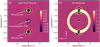 |
Fig. 1 (a) Final de-rotated image of the ϵ Indi A target with high-pass filter applied. (b) ADI processed image. |
4 Analysis
To quantify the results further, we calculated a background-noise-limited sensitivity and contrast curve using artificial planet injections and recovery tests for each target, which is discussed in the following sections.
4.1 Point-source contrast sensitivity
To compute the planet detection sensitivity, we injected artificial planets at various angular and radial (0.7″, 0.85″, 1″, 1.5″, 2″, 2.5″) separations. To estimate signal-to-noise (S/N), we used the approach of Mawet et al. (2014), as implemented in the open source Vortex image processing library (Gomez Gonzalez et al. 2017). We found that a S/N of 5 using the above criteria was sufficient to visually identify inserted artificial planets, as can be seen from Fig. 2. The figure shows injected planets at a contrast of 10−4 with respect to ϵ Indi A, with separations of 1″, 1.7″, 2.5″. Panel b shows their S/N estimates, which varies from 5–7 from the inner to the outer planets.
The overall contrast curve sensitivity was calculated by azimuthally averaging the contrast required to achieve a 5 σ S/N. We used a power-law function to fit the radial points to obtain final contrast curves. The contrast curves of all our targets are shown in Figs. 3a–d. The contrast at small separation is affected by the coronagraphic glow similarly to background-noise-limited sensitivity, except for the target of Sirius A, for the reason mentioned in the previous section.
Estimated contrasts of the known RV companions of ϵ Indi A and ϵ Eri are included in Fig. 3 for comparison. Planet fluxes in the NEAR filter are calculated from the ATMO 2020 spectral models (Phillips et al. 2020, see Sect. 4.3) assuming literature values for the planet mass ( MJ and 0.77 ± 0.2 MJ ) and the system age (
 Gyr and 0.7 ± 0.3 Gyr). These values are plotted by blue points in Fig. 3. Since the masses are determined by radial velocity, radius measurements are not available. Both the planet radii and temperatures are taken from the ATMO evolutionary models.
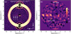 |
Fig. 2 (a) ϵ Indi A imagewith injected planets at a contrast of 10−4 with a separation from 1″ to 2.5″ marked with white arrows to left. On the right-hand side is a likely false positive identifiedfrom an examination of the odd-even frames. (b) S/N map showing injected planets appearing with the S/N in the 5–7 range. The approximate position of ϵ Indi Ab is shown by a circle, but the uncertainties are large (for details, see Feng et al. 2019). |
4.2 Background-noise-limited imaging performance (BLIP)
We obtaineda 5σ background-noise-limited imaging performance (BLIP) by calculating the standard deviation in 4-pix radius (=1.25λ∕D) apertures at various locations of the PCA-reduced images. This value was then multiplied by five times the square root of the number of pixels in the aperture ( ). To obtain the sensitivity with respect to the target, we used the off-axis stellar PSF for a relative flux calibration. This process was repeated for 20 angular and 17 radial distances separated by 7 pix. The mean of the angular values was then calculated to obtain a background-noise-limited sensitivity curve as shown by the dashed line in Figs. 3a–d.
The background-noise-limited sensitivity steeply increases at small separations (≲ 1″) for targets ϵ Indi A, ϵ Eri, and τ Ceti, which is due to the coronagraphic glow. Because the AGPM is not located downstream of a cold stop in VISIR, a part of the thermal emission originating from outside the telescope pupil (incl. the central obscuration) is diffracted back inside the pupil by the vortex effect (see Absil et al. 2016 for details). This creates a significant additional amount of thermal background close to the centre of the AGPM on the detector, which could be mitigated by introducing a cold stop upstream of the AGPM.
The BLIP sensitivity would only be reached in the absence of coronagraphic PSF residuals (quasi-static speckles; QSS) from the central star. It can be compared to the point-source sensitivity contrast introduced above to evaluate the angular separation beyond which BLIP sensitivity is reached. At such angular separations, the sensitivity improves with the square root of the integration time, while sensitivity improvements in the inner regions dominated by QSS are much harder to achieve.
Figures 3 and 4 show that the gap between BLIP sensitivity and point-source sensitivity contrast levels out at angular separations of around 1″ or 3.5 λ∕D for the fainter stars of our sample (ϵ Indi A, ϵ Eri, τ Ceti and Sirius B. At such separations, QSS are no longer seen (cf. Fig. 1) and pixel-pixel noise dominates the sensitivity. The shallow improvement of the point-source sensitivity towards even larger angular separations can be attributed to the PCA algorithm, which does not conserve flux and self-subtracts a diminishing fraction of the injected fake planet’s signal.
The contrast around the very bright Sirius A is instead limited by QSS and PSF residuals out to an angular separation of several arcseconds. This is due to a slight misalignment between the star and the coronagraph during the observation, and to the use of a conventional Lyot stop (LS). While the apodised LS used during the Alpha Cen observing campaign (Wagner et al. 2021) suppresses the off-axis Airy pattern at angular separations similar to the chopping throw of 4.5″, this conventional LS does not reduce the Airy pattern of the off-axis chopping position and leaves residuals near the coronagraphic centre, which reduces sensitivity.
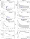 |
Fig. 3 Panels a-d show 5 σ contrast curves and background-noise-limited imaging performance. Panels e-h show the mass limits derived using contrast curves. The solid line is derived using artificial injection and recovery tests, and the thin line represents the 5 σ BLIP sensitivity. The detection limits would improve with |

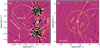 |
Fig. 4 (a) Final de-rotated image showing Sirius A and Sirius B. (b) Zoom-in on Sirius B, divided into two regions (inner and outer) based on the number of frames in the outlined area. |
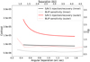 |
Fig. 5 SiriusB 5 σ contrast curves (same as in Fig. 3). The outer and inner regions are represented by red and black lines, respectively.The contrast curve for outer region increases at small separation due to edge of the inner frames. |
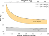 |
Fig. 6 Planet mass upper limits derived for Sirus B. The two mass limits are based on the outer and inner region (see Fig. 5). |
4.3 Mass limits
The contrast curves were converted into mass limits using the ATMO 2020 exoplanet atmosphere models (Phillips et al. 2020). The models are computed using a state-of-the-art, one-dimensional, radiative-convective equilibrium code along a grid of self-consistent pressure-temperature profiles and chemical equilibrium abundances for a range of effective temperatures (200–3000 K) and gravities (2.5–5.5 dex). ATMO 2020 has key improvements over previous model families, including the use of updated molecular line opacities which results in warmer atmospheric temperature structures and improved emission spectra. We used the non-equilibrium models with weak vertical mixing and the isochrones of age ranges obtained from literature to determine the masses corresponding to the contrast curves.
For absolute flux value of Sirius A, we use reported value from ESO’s list of mid-IR standard stars1. It provides a flux of 118.8 Jy in the PAH2 filter, which has the same central wavelength (11.25 μm) as the broad NEAR filter with a bandpass of 10–12.5 μm. For the other stars, we estimated the absolute flux from the tabulated K-band magnitude and applying the K–M correction from Allen’s astrophysical quantities (Cox 2000). The M–N colourof main-sequence stars with spectral type earlier than K5 is vanishingly small as this wavelength regime is well within the Rayleigh–Jeans part of the stellar spectrum. This procedure yields the 11.25 μm fluxes of ~ 4.5 Jy for ϵ Indi A, ~ 7.6 Jy for ϵ Eri, and ~ 7.5 Jy for τ Ceti. We also applied the procedure to some standard stars with tabulated K-band magnitude and PAH2 fluxes and found the values to agree within a few percent. For Sirius A, the estimate is 117 Jy, which is in very good agreement with the tabulated 118.8 Jy. We used Sirius A as a reference to calculate differential flux for other targets and find that the values agree with the calculation. We find no evidence of mid-IR excess in our targets consistent with the following previous works, Sirius A (White et al. 2019), Sirius B (Skemer & Close 2011), ϵ Indi A (Trilling et al. 2008), ϵ Eri (Backman et al. 2009) and τ Ceti (Lawler et al. 2014) are known to have some IR excess from their extended debris discs, but this emission is mostly from cold dust and therefore at longer wavelengths. Also, our high-spatial-resolution imagery would resolve the debris disc from the central star, such that no IR excess is measured on the central PSF.
5 Discussion
5.1 ϵ Indi A
To constrain the mass limits of companions to ϵ Indi A, we adopted an age range of 0.7–4 Gyr for our models and find limits of 3.3–10 MJ beyond 1′′. Since the mass of the known planet is  , MJ , we would have likely detected it if the age of the system were 0.7 Gyr, as shown in Fig. 3e. Our non-detection therefore supports an older age for ϵ Indi A. This is consistent with the majority of the age determinations, as discussed in the introduction above. We can calculate the requiredobservation time to detect the known giant planet by assuming a likely age of 3.8 Gyr in a background-limited regime and with improved sensitivity at small separations (without coronographic glow). Detecting the planet associated with the RV signal requires 50 h of observing time.
The limits we obtain are more sensitive than any previous near-IR imaging campaigns, which have constrained the masses of possible companions to 20 MJ in the inner regions of the system (Geißler et al. 2007) and 5–20 MJ at separations larger than 2′′ (Janson et al. 2009). Another independent reduction of ϵ Indi A combiningthe NEAR and NaCO L′ data reachessimilar mass limits to ours Viswanath, (in prep.).
ϵ Indi Ba andBb are not discussed in this paper as their wide orbit (1459 AU, Scholz et al. 2003; McCaughrean et al. 2004) corresponds to an approximately 6.7 arcmin separation, which is far outside the field of view of the VISIR instrument.
5.2 ϵ Eri
We adoptedan age range of 0.4–1 Gyr for our models. We obtained mass limits of 2–4 MJ , as shown in Fig. 3f. The obtained limits are more sensitive than most previous imaging data (Macintosh et al. 2003; Janson et al. 2008; Mizuki et al. 2016; Hunziker et al. 2020), with the exception of Mawet et al. (2019), who derived an upper mass limit of about 2 MJ for an assumed system age of 400 Myr. Reaching similar mass limits at different wavelengths does, however, reduce the dependency on the planet atmosphere models. Our result therefore increases the confidence that there is indeed no planet more massive than 2 MJ around ϵ Eri, for an age of 400 Myr old. The debris disc around ϵ Eri (Backman et al. 2009) is too large for our field of view and too cold and faint at 11.25 μm to be detected in our observations. To estimate the required observing time for detecting ϵ Eri b for a likely age of 0.7 Gyr, we find that 1 MJ planet can be detected in under 70 h with the current setup, and sensitivity will improve at small separations if the coronographic glow is eliminated (by introducing a cold pupil stop in front of the AGPM coronagraph mask).
5.3 τ Ceti
Because of the large age range suggested in the literature, we adopted a 3–10 Gyr range. The obtained mass limits of 15–30 MJ shown in Fig. 3g are comparable to those of Boehle et al. (2019), who used a combination of radial velocity and 3.8 μ m imaging data to find limits of 10–20 MJ beyond 2′′ for a slightly younger age range (2.9–8.7 Gyr). Within 2′′ our observation is more sensitive, and the non-detection of any of the known planets is consistent with the expectation, as the various Earth-mass planets of the system are far too low mass and are located within the inner working angle of our data, and even the proposed giant planet candidate is well below our detection threshold (1–2 MJ at 3–20 AU).
5.4 Sirius A
For our models, we assumed an age range of 0.2–0.3 Gyr for Sirius. For Sirius A, we also included the irradiation from the star when determining the expected magnitude of the planet, due to the brightness of the host star. We accounted for the irradiation by counting both the flux arriving at the planet surface and the intrinsic formation heat of the planet from the model as incoming energy when calculating the equilibrium temperature, which in turn determines the outgoing flux. Sirius A is 25 times more luminous than the Sun, and a potential planet on a 2 AU orbit would be heated to more than 400 K, independently of the planet’s age or mass.This leads to the peculiar shape of the mass contrast curve with better mass sensitivities at small separation from Sirius A, as shown in Fig. 3h. As a result, the curve of the mass limit falls of sharply within ~ 1′′ or 2.6 AU, where the stellar radiation dominates. Beyond this, the irradiation quickly becomes negligible as it falls off with the square of the distance, and the curve looks more similar to those of the other systems. The other systems have smaller, fainter stars, and therefore the amount of heating by the stellar flux is negligible at the separations resolved by our imagery. While we do not detect any planets, we do obtain the most sensitive mass limits to date within 1.5′′ and comparable limits to the most sensitive limits of previous imaging campaigns outside that radius (Bonnet-Bidaud & Pantin 2008; Thalmann et al. 2011; Vigan et al. 2015; Hunziker et al. 2020). We cannot rule out the possibility of planets that could be hidden behind or too close to the star.
5.5 Sirius B
No ADI reduction had to be applied to the Sirius B data, because the star is 4 × 10⁻⁵ times fainter than Sirius A and no PSF residuals are seen besides the PSF core. Additionally, the target was far from Sirius A and the noise of its coronagraphic PSF, so no further processing was necessary. The final image of Sirius A and B is shown in Fig. 4. Sirius B was very close to edge of the NEAR’s field of view, and even outside of it for some individual frames, which were then excluded before derotation and averaging. To calculate the sensitivity around Sirius B, we divided that area of the image into two regions, an inner and an outer region, as shown in Fig. 4b. The inner region provides a better sensitivity for both the background-noise-limited and injected planet, as it includes more frames as shown in Fig. 5.
The astrometry measurements for Sirius B put it at a separation of 11.18″ from Sirius A. Relative photometry with respect to Sirius A was performed using an optimum r = 4 pix photometric aperture. The 11.25 μm contrast ratio between the two stars is 4 × 10⁻⁵, corresponding to a Sirius B flux of 4.7 mJy at a S/N of about 40. This value is consistent with the low S/N measurement of 4.9 mJy reported for a similar observing band by Skemer & Close (2011).
For our models, we assumed the same age range as we did for Sirius A, giving us limits of 1.5–1.8 MJ for the ‘inner’ region and 3.1–3.6 MJ for the ‘outer’ region as shown in Fig. 6. The mass limits in the inner region are comparable to previous near-IR limits of 1.6 MJ from Thalmann et al. (2011). According to the models and assuming the sensitivity improving with  , a four times longer observation time would be enough to reach 0.5 MJ .
6 Summary and conclusions
In this work we demonstrate high-contrast imaging of a small sample of very nearby (<4 pc) stars with spectral types earlier than M at 11.25 μm with NEAR. While we do not detect any known or new planets, we were able to set upper mass limits of the order of a few Jupiter masses for most of the targets and of 15–30 MJ for the older τ Ceti. For ϵ Indi A and ϵ Eri, we achieve detection limits very close to the giant planets discovered by RV, with the limits on ϵ Indi A being the most sensitive to date. For τ Ceti and Sirius A, we obtain the most sensitive limits to date at small separations (< 1.5′′ and < 2′′, respectively). Our mass limit for Sirius B is similar to the one achieved previously at a shorter wavelength.
The ADI analysis was performed using a PCA-based algorithm with artificial planet injections and recovery tests yielding some of the most stringent upper mass limits to date. For ϵ Indi A and ϵ Eri, we almost reached the detection limit for the known planets if they were at the young end of the possible age estimates, but we failed to detect any signal. We achieved an unprecedented sub-mJy detection sensitivity.
We demonstrate close to background-noise-limited imaging for most of our target stars apart from the glaring Sirius A, for which the data is contrast limited. Assuming likely ages and background-noise-limited imaging, the giant planets orbiting ϵ Eri and ϵ Indi A can be imaged in 70 and 50 h, respectively. Finally, for our closest and youngest (together with Sirius A) target Sirius B, the sub-Jupiter mass regime could be reached by merely doubling the observation time.
This work shows the potential of direct imaging in the mid-IR regime and prospects for upcoming mid-IR HCI instruments. Upcoming mid-IR HCI instrument such as METIS at the ELT would be able to detect known planets around ϵ Indi A and ϵ Eri in a few minutes of observation time and reach sensitivities to detect Earth-sized exoplanets in a few hours (Brandl et al. 2018).
Acknowledgements
The authors would like to thank the ESO and the Breakthrough Foundation and all the people involved for making the NEAR project possible. The observations were carried out under the ESO program id: 60.A-9107(D) and 60.A-9107(F). MRM acknowledges the support of a grant from the Templeton World Charity Foundation, Inc. The opinions expressed in this publication are those of the authors and do not necessarily reflect the views of the Templeton World Charity Foundation, Inc. Part of this work has received funding from the European Research Council (ERC) under the European Union’s Horizon 2020 research and innovation programme (grant agreement No. 819155), and by the Wallonia-Brussels Federation (grant for Concerted Research Actions).
References
- Absil, O., Mawet, D., Karlsson, M., et al. 2016, in Society of Photo-Optical Instrumentation Engineers (SPIE) Conference Series, 9908, Ground-based and Airborne Instrumentation for Astronomy VI, eds. C. J. Evans, L. Simard, & H. Takami, 99080Q [Google Scholar]
- Arrington, D. C., Hubbs, J. E., Gramer, M. E., & Dole, G. A. 1998, in Society of Photo-Optical Instrumentation Engineers (SPIE) Conference Series, 3379, Infrared Detectors and Focal Plane Arrays V, eds. E. L. Dereniak, & R. E. Sampson, 361 [Google Scholar]
- Arsenault, R., Madec, P. Y., Vernet, E., et al. 2017, The Messenger, 168, 8 [Google Scholar]
- Backman, D., Marengo, M., Stapelfeldt, K., et al. 2009, ApJ, 690, 1522 [NASA ADS] [CrossRef] [Google Scholar]
- Baraffe, I., Chabrier, G., Barman, T. S., Allard, F., & Hauschildt, P. H. 2003, A&A, 402, 701 [NASA ADS] [CrossRef] [EDP Sciences] [Google Scholar]
- Benedict, G. F., McArthur, B. E., Gatewood, G., et al. 2006, AJ, 132, 2206 [Google Scholar]
- Beuzit, J. L., Vigan, A., Mouillet, D., et al. 2019, A&A, 631, A155 [NASA ADS] [CrossRef] [EDP Sciences] [Google Scholar]
- Boehle, A., Quanz, S. P., Lovis, C., et al. 2019, A&A, 630, A50 [NASA ADS] [CrossRef] [EDP Sciences] [Google Scholar]
- Bond, H. E., Schaefer, G. H., Gilliland, R. L., et al. 2017, ApJ, 840, 70 [NASA ADS] [CrossRef] [Google Scholar]
- Bonnet-Bidaud, J. M., & Pantin, E. 2008, A&A, 489, 651 [EDP Sciences] [Google Scholar]
- Booth, M., Dent, W. R. F., Jordán, A., et al. 2017, MNRAS, 469, 3200 [Google Scholar]
- Brandl, B. R., Absil, O., Agócs, T., et al. 2018, in Society of Photo-Optical Instrumentation Engineers (SPIE) Conference Series, 10702, Ground-based and Airborne Instrumentation for Astronomy VII, eds. C. J. Evans, L. Simard, & H. Takami, 107021U [Google Scholar]
- Burleigh, M. R., Clarke, F. J., & Hodgkin, S. T. 2002, MNRAS, 331, L41 [Google Scholar]
- Chauvin, G., Desidera, S., Lagrange, A. M., et al. 2017, A&A, 605, A9 [EDP Sciences] [Google Scholar]
- Cox, A. N. 2000, Allen’s astrophysical quantities [Google Scholar]
- Dietrich, J., & Apai, D. 2021, AJ, 161, A17 [Google Scholar]
- Dieterich, S. B., Weinberger, A. J., Boss, A. P., et al. 2018, ApJ, 865, 28 [NASA ADS] [CrossRef] [Google Scholar]
- Di Folco, E., Thévenin, F., Kervella, P., et al. 2004, A&A, 426, 601 [NASA ADS] [CrossRef] [EDP Sciences] [Google Scholar]
- Eker, Z., Soydugan, F., Soydugan, E., et al. 2015, AJ, 149, 131 [NASA ADS] [CrossRef] [Google Scholar]
- Endl, M., Kürster, M., Els, S., et al. 2002, A&A, 392, 671 [NASA ADS] [CrossRef] [EDP Sciences] [Google Scholar]
- Feng, F., Tuomi, M., Jones, H. R. A., et al. 2017, AJ, 154, 135 [Google Scholar]
- Feng, F., Anglada-Escudé, G., Tuomi, M., et al. 2019, MNRAS, 490, 5002 [NASA ADS] [CrossRef] [Google Scholar]
- Fortney, J. J., Lodders, K., Marley, M. S., & Freedman, R. S. 2008, ApJ, 678, 1419 [NASA ADS] [CrossRef] [Google Scholar]
- Friedrich, S., Zinnecker, H., Correia, S., et al. 2007, in Astronomical Society of the Pacific Conference Series, 372, 15th European Workshop on White Dwarfs, eds. R. Napiwotzki, & M. R. Burleigh, 343 [Google Scholar]
- Gaia Collaboration (Brown, A. G. A., et al.) 2021, A&A 650, C3 [EDP Sciences] [Google Scholar]
- Gänsicke, B. T., Schreiber, M. R., Toloza, O., et al. 2019, Nature, 576, 61 [NASA ADS] [CrossRef] [Google Scholar]
- Geißler, K., Kellner, S., Brandner, W., et al. 2007, A&A, 461, 665 [NASA ADS] [CrossRef] [EDP Sciences] [Google Scholar]
- Gomez Gonzalez, C. A., Wertz, O., Absil, O., et al. 2017, AJ, 154, 7 [Google Scholar]
- Gratton, R., D’Orazi, V., Pacheco, T. A., et al. 2021, A&A, 646, A61 [EDP Sciences] [Google Scholar]
- Gray, R. O., Corbally, C. J., Garrison, R. F., et al. 2006, AJ, 132, 161 [NASA ADS] [CrossRef] [Google Scholar]
- Greaves, J. S., Wyatt, M. C., Holland, W. S., & Dent, W. R. F. 2004, MNRAS, 351, L54 [Google Scholar]
- Hatzes, A. P., Cochran, W. D., McArthur, B., et al. 2000, ApJ, 544, L145 [Google Scholar]
- Henry, T. J., Soderblom, D. R., Donahue, R. A., & Baliunas, S. L. 1996, AJ, 111, 439 [NASA ADS] [CrossRef] [Google Scholar]
- Hunziker, S., Schmid, H. M., Mouillet, D., et al. 2020, A&A, 634, A69 [CrossRef] [EDP Sciences] [Google Scholar]
- Janson, M., Reffert, S., Brandner, W., et al. 2008, A&A, 488, 771 [NASA ADS] [CrossRef] [EDP Sciences] [Google Scholar]
- Janson, M., Apai, D., Zechmeister, M., et al. 2009, MNRAS, 399, 377 [NASA ADS] [CrossRef] [Google Scholar]
- Janson, M., Quanz, S. P., Carson, J. C., et al. 2015, A&A, 574, A120 [NASA ADS] [CrossRef] [EDP Sciences] [Google Scholar]
- Jovanovic, N., Martinache, F., Guyon, O., et al. 2015, PASP, 127, 890 [NASA ADS] [CrossRef] [Google Scholar]
- Kasper, M., Burrows, A., & Brandner, W. 2009, ApJ, 695, 788 [NASA ADS] [CrossRef] [Google Scholar]
- Kasper, M., Arsenault, R., Käufl, H. U., et al. 2017, The Messenger, 169, 16 [NASA ADS] [Google Scholar]
- Kasper, M., Arsenault, R., Käufl, U., et al. 2019, The Messenger, 178, 5 [Google Scholar]
- Keppler, M., Benisty, M., Müller, A., et al. 2018, A&A, 617, A44 [NASA ADS] [CrossRef] [EDP Sciences] [Google Scholar]
- Kervella, P., Arenou, F., Mignard, F., & Thévenin, F. 2019, A&A, 623, A72 [NASA ADS] [CrossRef] [EDP Sciences] [Google Scholar]
- King, R. R., McCaughrean, M. J., Homeier, D., et al. 2010, A&A, 510, A99 [NASA ADS] [CrossRef] [EDP Sciences] [Google Scholar]
- Lachaume, R., Dominik, C., Lanz, T., & Habing, H. J. 1999, A&A, 348, 897 [NASA ADS] [Google Scholar]
- Lagage, P. O., Pel, J. W., Authier, M., et al. 2004, The Messenger, 117, 12 [NASA ADS] [Google Scholar]
- Lawler, S. M., Di Francesco, J., Kennedy, G. M., et al. 2014, MNRAS, 444, 2665 [Google Scholar]
- Liebert, J., Young, P. A., Arnett, D., Holberg, J. B., & Williams, K. A. 2005, ApJ, 630, L69 [NASA ADS] [CrossRef] [Google Scholar]
- MacGregor, M. A., Lawler, S. M., Wilner, D. J., et al. 2016, ApJ, 828, 113 [Google Scholar]
- Macintosh, B. A., Becklin, E. E., Kaisler, D., Konopacky, Q., & Zuckerman, B. 2003, ApJ, 594, 538 [NASA ADS] [CrossRef] [Google Scholar]
- Macintosh, B., Graham, J. R., Ingraham, P., et al. 2014, Proc. Nat. Acad. Sci., 111, 12661 [Google Scholar]
- Macintosh, B., Graham, J. R., Barman, T., et al. 2015, Science, 350, 64 [NASA ADS] [CrossRef] [Google Scholar]
- Maire, A.-L., Huby, E., Absil, O., et al. 2020, J. Astron. Telescopes Instrum. Syst., 6, 1 [Google Scholar]
- Mamajek, E. E., & Hillenbrand, L. A. 2008, ApJ, 687, 1264 [NASA ADS] [CrossRef] [Google Scholar]
- Marley, M. S., Fortney, J. J., Hubickyj, O., Bodenheimer, P., & Lissauer, J. J. 2007, ApJ, 655, 541 [Google Scholar]
- Marois, C., Lafrenière, D., Doyon, R., Macintosh, B., & Nadeau, D. 2006, ApJ, 641, 556 [Google Scholar]
- Marois, C., Macintosh, B., Barman, T., et al. 2008, Science, 322, 1348 [NASA ADS] [CrossRef] [PubMed] [Google Scholar]
- Mawet, D., Riaud, P., Absil, O., & Surdej, J. 2005, ApJ, 633, 1191 [NASA ADS] [CrossRef] [Google Scholar]
- Mawet, D., Milli, J., Wahhaj, Z., et al. 2014, ApJ, 792, 97 [NASA ADS] [CrossRef] [Google Scholar]
- Mawet, D., Hirsch, L., Lee, E. J., et al. 2019, AJ, 157, 33 [NASA ADS] [CrossRef] [Google Scholar]
- McCaughrean,M. J., Close, L. M., Scholz, R. D., et al. 2004, A&A, 413, 1029 [NASA ADS] [CrossRef] [EDP Sciences] [Google Scholar]
- Meyer, M. R., Currie, T., Guyon, O., et al. 2018, ArXiv e-prints [arXiv:1804.03218] [Google Scholar]
- Mizuki, T., Yamada, T., Carson, J. C., et al. 2016, A&A, 595, A79 [NASA ADS] [CrossRef] [EDP Sciences] [Google Scholar]
- Nowak, M., Lacour, S., Lagrange, A. M., et al. 2020, A&A, 642, A2 [CrossRef] [EDP Sciences] [Google Scholar]
- Pagano, M., Truitt, A., Young, P. A., & Shim, S.-H. 2015, ApJ, 803, 90 [Google Scholar]
- Phillips, M. W., Tremblin, P., Baraffe, I., et al. 2020, A&A, 637, A38 [NASA ADS] [CrossRef] [EDP Sciences] [Google Scholar]
- Quanz, S. P., Crossfield, I., Meyer, M. R., Schmalzl, E., & Held, J. 2015, Int. J. Astrobiol., 14, 279 [CrossRef] [Google Scholar]
- Scholz, R. D., McCaughrean, M. J., Lodieu, N., & Kuhlbrodt, B. 2003, A&A, 398, L29 [NASA ADS] [CrossRef] [EDP Sciences] [Google Scholar]
- Skemer, A. J.,& Close, L. M. 2011, ApJ, 730, 53 [Google Scholar]
- Song, I., Caillault, J. P., Barrado y Navascués, D., Stauffer, J. R., & Randich, S. 2000, ApJ, 533, L41 [NASA ADS] [CrossRef] [PubMed] [Google Scholar]
- Spiegel, D. S.,& Burrows, A. 2012, ApJ, 745, 174 [Google Scholar]
- Sudarsky, D., Burrows, A., & Hubeny, I. 2003, ApJ, 588, 1121 [Google Scholar]
- Tang, Y. K., & Gai, N. 2011, A&A, 526, A35 [NASA ADS] [CrossRef] [EDP Sciences] [Google Scholar]
- Thalmann, C., Usuda, T., Kenworthy, M., et al. 2011, ApJ, 732, L34 [NASA ADS] [CrossRef] [Google Scholar]
- Trilling, D. E., Bryden, G., Beichman, C. A., et al. 2008, ApJ, 674, 1086 [NASA ADS] [CrossRef] [Google Scholar]
- Tuomi, M., Jones, H. R. A., Jenkins, J. S., et al. 2013, A&A, 551, A79 [NASA ADS] [CrossRef] [EDP Sciences] [Google Scholar]
- Turchi, A., Masciadri, E., Pathak, P., & Kasper, M. 2020, MNRAS, 497, 4910 [Google Scholar]
- Vanderburg, A., Rappaport, S. A., Xu, S., et al. 2020, Nature, 585, 363 [Google Scholar]
- Vigan, A., Gry, C., Salter, G., et al. 2015, MNRAS, 454, 129 [NASA ADS] [CrossRef] [Google Scholar]
- Wagner, K., Boehle, A., Pathak, P., et al. 2021, Nat. Commun., 12, 922 [Google Scholar]
- Walker, G. A. H., Walker, A. R., Irwin, A. W., et al. 1995, Icarus, 116, 359 [NASA ADS] [CrossRef] [Google Scholar]
- White, J. A., Aufdenberg, J., Boley, A. C., et al. 2019, ApJ, 875, 55 [Google Scholar]
- Zechmeister, M., Kürster, M., Endl, M., et al. 2013, A&A, 552, A78 [NASA ADS] [CrossRef] [EDP Sciences] [Google Scholar]
All Tables
All Figures
|
Fig. 1 (a) Final de-rotated image of the ϵ Indi A target with high-pass filter applied. (b) ADI processed image. |
| In the text | |
|
Fig. 2 (a) ϵ Indi A imagewith injected planets at a contrast of 10−4 with a separation from 1″ to 2.5″ marked with white arrows to left. On the right-hand side is a likely false positive identifiedfrom an examination of the odd-even frames. (b) S/N map showing injected planets appearing with the S/N in the 5–7 range. The approximate position of ϵ Indi Ab is shown by a circle, but the uncertainties are large (for details, see Feng et al. 2019). |
| In the text | |
|
Fig. 3 Panels a-d show 5 σ contrast curves and background-noise-limited imaging performance. Panels e-h show the mass limits derived using contrast curves. The solid line is derived using artificial injection and recovery tests, and the thin line represents the 5 σ BLIP sensitivity. The detection limits would improve with |
| In the text | |
|
Fig. 4 (a) Final de-rotated image showing Sirius A and Sirius B. (b) Zoom-in on Sirius B, divided into two regions (inner and outer) based on the number of frames in the outlined area. |
| In the text | |
|
Fig. 5 SiriusB 5 σ contrast curves (same as in Fig. 3). The outer and inner regions are represented by red and black lines, respectively.The contrast curve for outer region increases at small separation due to edge of the inner frames. |
| In the text | |
|
Fig. 6 Planet mass upper limits derived for Sirus B. The two mass limits are based on the outer and inner region (see Fig. 5). |
| In the text | |
Current usage metrics show cumulative count of Article Views (full-text article views including HTML views, PDF and ePub downloads, according to the available data) and Abstracts Views on Vision4Press platform.
Data correspond to usage on the plateform after 2015. The current usage metrics is available 48-96 hours after online publication and is updated daily on week days.
Initial download of the metrics may take a while.