| Issue |
A&A
Volume 652, August 2021
|
|
|---|---|---|
| Article Number | A80 | |
| Number of page(s) | 11 | |
| Section | Extragalactic astronomy | |
| DOI | https://doi.org/10.1051/0004-6361/202140526 | |
| Published online | 13 August 2021 | |
New constraints on the magnetic field in cosmic web filaments⋆
1
Dipartimento di Fisica e Astronomia, Universitá di Bologna, Via Gobetti 93/2, 40122 Bologna, Italy
e-mail: This email address is being protected from spambots. You need JavaScript enabled to view it.
2
Istituto di Radioastronomia, INAF, Via Gobetti 101, 40122 Bologna, Italy
3
Max-Planck-Institut für Extraterrestrische Physik (MPE), Giessenbachstrasse 1, 85748 Garching bei München, Germany
e-mail: This email address is being protected from spambots. You need JavaScript enabled to view it.
4
Hamburger Sternwarte, University of Hamburg, Gojenbergsweg 112, 21029 Hamburg, Germany
5
Department of Physics and Electronics, Rhodes University, PO Box 94 Grahamstown 6140, South Africa
6
South African Radio Astronomy Observatory, Black River Park, 2 Fir Street, Observatory, Cape Town 7925, South Africa
7
Leiden Observatory, Leiden University, PO Box 9513 2300 RA Leiden, The Netherlands
8
ASTRON, The Netherlands Institute for Radio Astronomy, Postbus 2, 7990 AA Dwingeloo, The Netherlands
Received:
10
February
2021
Accepted:
15
May
2021
Abstract
Strong accretion shocks are expected to illuminate the warm–hot intergalactic medium encompassed by the filaments of the cosmic web, through synchrotron radio emission. Given their high sensitivity, large low-frequency radio facilities may already be able to detect signatures of this extended radio emission from the region between two close and massive galaxy clusters. In this work we exploit the non-detection of such diffuse emission by deep observations of two pairs of relatively close (≃10 Mpc) and massive (M500 ≥ 1014 M⊙) galaxy clusters using the LOw-Frequency ARray. By combining the results from the two putative inter-cluster filaments, we derive new independent constraints on the median strength of intergalactic magnetic fields: B10 Mpc < 2.5 × 10² nG (95% confidence level). Based on cosmological simulations and assuming a primordial origin of the B-fields, these estimates can be used to limit the amplitude of primordial seed magnetic fields: B0 ≤ 10 nG. We recommend the observation of similar cluster pairs as a powerful tool to set tight constraints on the amplitude of extragalactic magnetic fields.
Key words: magnetic fields / acceleration of particles / galaxies: clusters: general
The code used to produce the simulations discussed in this paper is public (https://enzo-project.org). Significant subsets of the simulations are publicly available at https://cosmosimfrazza.myfreesites.net/the_magnetic_cosmic_web, while larger data sets can be shared upon request.
© ESO 2021
1. Introduction
On the largest scales of the Universe (≥10 Mpc), galaxy groups and clusters are connected by elongated distributions of galaxies called filaments and sheets which are also believed to be permeated by diffuse gas, and possibly by magnetic fields. To date, a straightforward and direct detection of intergalactic medium (IGM) and an intergalactic magnetic field (IGMF) has been prevented by the very low density of the plasma (nIGM ≤ 10−4 cm−3) and its relatively low temperature (TIGM ≤ 107 K). However, increasing evidence (Nicastro et al. 2018; Macquart et al. 2020; Tanimura et al. 2020) is confirming the long-lived expectations for the warm–hot gas phase of the IGM (WHIM, with TWHIM ∼ 105 − 107, nWHIM ∼ 10−5 − 10−4) to contain up to half of the baryon content at low redshifts (Cen & Ostriker 1999; Davé et al. 2001; Reiprich et al. 2021).
Accretion shocks are believed to reside along and within the filaments of the cosmic web and at the outskirts of galaxy clusters. These shocks are expected to amplify the magnetic fields and to accelerate particles up to relativistic energies (Ryu et al. 2008). Their presence might then enable the detection of the WHIM through its synchrotron emission signature at radio wavelengths, and indeed the direct observation of the tip of the iceberg of this diffuse emission has already been obtained at radio frequencies (Govoni et al. 2019; Botteon et al. 2020a). In these few cases the plasma conditions are still hotter and denser than was expected for the WHIM, and the detected emission lays within the clusters virial radii. Further works in this direction will be helped in the near future by the promising new and upcoming radio facilities (the next generation Very Large Array, ngVLA; the Karoo Array Telescope, MeerKAT; the square kilometer array SKA-mid) and especially at very low frequencies (the LOw-Frequency, ARray LOFAR; the Murchison Widefield Array, MWA; SKA-low) where the emission should be brighter up to further out the clusters virial radii thanks to the expected spectral behaviour as Sν ∝ ν−1 with respect to frequency ν (Vazza et al. 2015). A way to overcome sensitivity limitations is to quantify the Faraday effect induced by magneto-ionised plasma along the line of sight to a polarised background radio source, and to build a tomography of the WHIM by means of a grid of background sources (see Akahori et al. 2014; Vacca et al. 2016). A thorough exploitation of this method currently suffers from the lack of large and dense grids of polarised sources; however, it is expected to provide important results thanks to the upcoming radio facilities (Locatelli et al. 2018). Recent upper limits on the IGMF intensity and scale were derived from the cross-correlation of diffuse radio synchrotron emission with the underlying galaxy distribution (Vernstrom et al. 2017; Brown et al. 2017) by cross-correlating the difference in rotation measures of physically related pairs of extended radio galaxies, compared with that derived from randomly paired close lobes (Vernstrom et al. 2019; O’Sullivan et al. 2020; Stuardi et al. 2020) and by stacking full sky low-frequency radio images of close red luminous galaxy pairs (Vernstrom et al. 2021).
The question arises of why it is important to assess the IGMF properties in the cosmic web at late times. The magnetic fields in galaxies and galaxy clusters, commonly observed today, arise from strong amplification from efficient magnetohydrodynamic (MHD) small-scale mechanisms (Ryu et al. 2008) that are responsible for a fast saturation of the fields, thus erasing information of their initial conditions, and in turn their origins (Beresnyak & Miniati 2016). Instead, in the WHIM environment the amplification of primordial magnetic fields is found in simulations to be mainly driven by the field compression as its lines freeze into the plasma plus the contribution of small scale shocks. These mechanisms do not bring the field to saturation, and provide a tool of assessing the history and original conditions of the field by means of the level of magnetisation observed today (Vazza et al. 2014, 2015; Donnert et al. 2018). For the above reasons it is crucial to constrain the magnetic field in the WHIM in order to determine the original scenario for the large-scale magnetic field origin and evolution in the Universe.
Cosmological MHD simulations predict the intensity of the IGMF at low redshift to be in the range between 1 and 100 nG (Dolag et al. 1999; Brüggen et al. 2005; Vazza et al. 2017). In this paper we introduce a novel method for a robust inference of an upper limit on the initial B0 and current B values of the IGMF within the large-scale filaments of the cosmic web. The method explores the amount of diffuse emission detected at 144 MHz with the LOw Frequency ARray (LOFAR) telescope along the direction connecting two different pairs of galaxy clusters.
We outline the method used to explore the upper limits on the IGMF into cosmological filaments in Sect. 2; we show its results in Sect. 3 and discuss their assumptions and implications in Sect. 4; and we draw our conclusions in Sect. 5. Throughout this work we assume a ΛCDM cosmological model with baryonic, dark matter, and dark energy density parameters ΩBM = 0.0455, ΩDM = 0.2265, and ΩΛ = 0.728, respectively, and a Hubble constant H0 = 70.2 km s−1 Mpc−1.
2. Method
In order to look for large-scale emission from the cosmic web, we observed pairs of galaxy clusters and the putative inter-cluster filaments connecting them. The cluster pairs were selected from the Meta-Catalogue of X-ray Detected Clusters of Galaxies1 (MCXC, Piffaretti et al. 2011) by applying cuts in declination (δ ≥ 10 deg), redshift (z ≤ 0.3), and maximum angular separation (θ ≤ 5 deg). These values were tailored to the proposed LOFAR observations. The two most promising pairs that, according to cosmological simulations, maximise the probability of a physical connection between the clusters in terms of total mass and separation (real and projected), were proposed and observed at the LOFAR during Cycle 9 (Proposal Id:LC9_020). The most important properties of the two observed pairs of clusters are given in Table 1.
Main parameters of the two pairs of galaxy clusters observed in this work, based on the Meta-Catalogue of X-ray Detected Clusters of Galaxies (MCXC; Piffaretti et al. 2011).
In a nutshell, after calibrating, imaging, and removing contaminating sources from the LOFAR data, we quantify the confidence of having observed (or not) diffuse emission from the inter-cluster filaments. We inject simulated diffuse emission produced by large-scale accretion shocks (≥Mpc), into the original radio visibility data (uvw) for a large subset (𝒪(100)) of simulated filaments and cluster pairs and image them, as done for the real observations.
In this section we provide further details of the analysis performed on the actual observations, the simulated data set prepared for the injection, and the injection procedure (see diagram in Fig. 1).
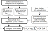 |
Fig. 1. Diagram of the method outlined in Sect. 2. The thick boxes highlight the most computationally expensive steps. Links labelled ‘i’ are computed iteratively over the simulated pairs. |
2.1. LOFAR radio observations
We observed the two cluster pairs RXCJ1659.7+3236−RXCJ1702.7+3403 (hereafter RXC_J1659−J1702) and RXCJ1155.3+2324−RXCJ1156.9+2415 (hereafter RXC_J1155−J1156) using LOFAR. The fields containing these two targets were co-observed with two pointings of the LOFAR Two-metre Sky Survey (LoTSS; Shimwell et al. 2017) taking advantage of the multi-beam capabilities of LOFAR. The observing set-up of our observations thus follows that of LoTSS, namely 8 h on-source time between two 10 min scans on the flux density calibrator in the frequency range 120−168 MHz using LOFAR in HBA_DUAL_INNER mode (see Shimwell et al. 2017, for details). A first calibration and imaging run was performed adopting the pipelines developed to analyse the LoTSS pointings (Shimwell et al. 2017, 2019); the aim was to correct for direction-independent and for direction-dependent effects exploiting the PREFACTOR (Williams et al. 2016; van Weeren et al. 2016; de Gasperin et al. 2019), KILLMS (Tasse 2014a,b; Smirnov & Tasse 2015), and DDFACET (Tasse et al. 2018) software. In particular, we used the improved version of the direction-dependent data reduction pipeline (v2.22), the same used for the forthcoming second LoTSS data release (DR2; Shimwell et al., in prep.) to produce images of the full LOFAR field of view at the central frequency of 144 MHz at high (6″) and low resolution (20″, shown in Fig. 2) using a Briggs weighting scheme (robust = −0.5). We refer the reader to Tasse et al. (2021) for a thorough description of the steps performed by the pipeline. Using the sky models derived from the pipeline, we subtracted the sources from the uv-data in two different fashions: either we subtracted all sources (by means of their clean components) found in the high- and low-resolution maps or we subtracted all sources detected in the high-resolution image. The model components were determined during the high- and low-resolution images deconvolution making use of the PYthon Blob Detector and Source Finder (PYBDSF; Mohan & Rafferty 2015). The subtraction of the model components was performed in the visibility domain, corrupting the model components by the direction-independent antenna gains obtained from the calibration. We then produced dirty images from the subtracted data. The images include the residual contribution to the surface brightness resulting from model approximation plus artefacts associated with imperfect model, and solutions (Imempty) plus patches of faint extended emission in the case when only sources from the high-resolution model were subtracted (Imdiffuse). The subtracted (dirty) images Imempty at low resolution (20″) have an rms noise floor of ∼160 and 240 μJy beam−1 for the two fields, respectively. The noise difference is consistent with the amount of flagged (i.e. discarded) data in the two observations.
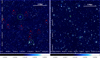 |
Fig. 2. LOFAR low-resolution (20″) images at 150 MHz of the cluster pairs RXC_J1659−J1702 (left panel) and RXC_J1155−J1156 (right panel). The dashed circles are centred on the clusters and have corresponding radius R500. Magnified images of the red dashed boxes in the left panel are shown in Fig. 8. The 5 Mpc unit at the redshift of the pairs z = 0.10, 0.14 is shown in the top right corner (left and right panels). The colour bars are in units of Jy beam−1. |
2.2. Cosmological simulations
We extracted the simulated inter-cluster filaments from the suite of simulations of the cosmic web properties described in Vazza et al. (2019) performed with the cosmological MHD code ENZO3 (Bryan et al. 2014). The simulations consist of a comoving 1003 Mpc3 box with a uniform grid of 24003 cells (and 24003 dark matter particles) with linear (comoving) resolution of 41.6 kpc per cell and dark matter mass mdm = 8.62 × 10⁶ M⊙ per dark matter particle. Magnetic fields are initialised at z = 45 as a uniform background of B0 = 0.1 nG and evolved at run-time using the MHD method of Dedner (Dedner et al. 2002). We note that a uniform initial magnetic field here corresponds to a scale-invariant spectrum in the models used for cosmic microwave background (CMB) analysis (Aghanim et al. 2019; Paoletti & Finelli 2019). We also note that the run is non-radiative and does not include any treatment for star formation or feedback from active galactic nuclei (AGN). While to a first approximation these processes are not very relevant for the radio and X-ray properties of the peripheral regions of galaxy clusters and filaments (e.g. Gheller & Vazza 2019), the effect of outflows from AGN and galaxies can mix metals and magnetic fields at least out to the virial radius of clusters (e.g. Biffi et al. 2018). Simulations by our group show that these effects are negligible on the radio emission on the scale of filaments (Vazza et al. 2017); however, only future and more refined simulations including effects related to galaxy formation in filaments at a much higher resolution, will be able to assess with more certainty whether the limits obtained from observations (such as those obtained in this work) can be straightforwardly related to a limit on primordial seed fields.
2.3. Synchrotron emission model for cosmic shocks
We produced synthetic maps of synchrotron radio emission assuming that diffusive shock acceleration (DSA; e.g. Kang et al. 2012 and references therein) accelerates a small fraction of thermal electrons swept by structure formation shocks up to relativistic energies, as in Vazza et al. (2019). We computed the radio emission from electrons in the downstream cooling region of shocks using the model of Hoeft & Brüggen (2007), and based on the shocks identified in post-processing in the simulation. The total acceleration efficiency at shocks, ξe(ℳ) (with ℳ the Mach number) is assumed to be the combination of two variables: the kinetic energy flux dissipated onto the acceleration of cosmic rays, ψ(ℳ), and the fraction going into electron acceleration,  , giving
 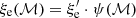 . Following Hoeft & Brüggen (2007), the radio emission in the downstream of each shock is directly linked to the power-law energy distributions Nγ ∝ γ−p of electrons accelerated by the shock front during a cooling time through the integrated radio spectrum of I(ν) ∝ ν−s, where s = (p − 1)/2 + 1/2, with p = 2(ℳ2 + 1)/(ℳ2 − 1). With this approach and for the range of ℳ ≫ 5 shocks usually found within and around simulated filaments, and for the ≤μG magnetic fields in filaments (e.g. Vazza et al. 2017), the radio emission thus scales as I(ν) ∝ ξeB2ν−2. The baseline model used in this work assumes ξe = 10−2, which is in line with DSA expectations for the maximum acceleration efficiency of relativistic electrons by strong shocks (e.g. Hoeft & Brüggen 2007; Kang et al. 2012; Bykov et al. 2019a) and is also compatible with the modelling of supernova remnants (e.g. Uchiyama et al. 2007; Bykov et al. 2019b). However, in typically weak shocks (ℳ ≤ 4) leading to radio relics in galaxy clusters (e.g. van Weeren et al. 2019) the acceleration efficiencies implied by the observed relic radio fluxes can be much larger (ξe ∼ 0.1−1; see e.g. Stuardi et al. 2019; Botteon et al. 2020b), thus making our maximum value of ξe = 10−2 a conservative one. We note, however, that very recent particle-in-cell (PIC) simulations (albeit in 1D and with some limiting assumptions) derive a ∼5% electron acceleration efficiency by strong shocks (Xu et al. 2020). For the remainder of the paper it should be kept in mind that our limits on B10 Mpc must be accordingly rescaled if a different value of ξe is adopted.
Figure 3 gives an example of filaments connecting a massive cluster to other groups in its surrounding, in an ENZO cosmological simulation. A small but significant fraction of radio emission from shocks running on filaments connecting some of the pairs (e.g. M1−M2, M1−M4, and M1−M6 in Fig. 3) is above the detection threshold in LOFAR-HBA for our baseline model. In all cases the detectable emission comes from relatively small and localised patches, extended a few ≃10′−20′ at most, with irregular shapes. Detecting the radio signal from cosmic filaments is indeed made challenging by the fact that the detectable fraction is just the tip of the iceberg of the wider ‘radio cosmic web’, which often makes a morphological classification of the emission ambiguous. Advanced Deep Learning techniques have been proposed for the detection of the cosmic web in future radio surveys (Gheller et al. 2018). In the following section we use this model to constrain the amplitude of the ξeB2 combination based on our real LOFAR observations.
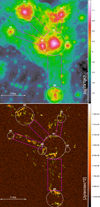 |
Fig. 3. Example of mean gas temperature (top) and mock LOFAR-HBA observation (bottom, ν = 140 MHz, 25″ resolution, 250 μJy beam−1 noised added) from the ENZO simulation. The circles indicate the virial region of clusters; the magenta rectangles show the filaments. The detectable emission (≥3σ) is shown as green contours. The cluster field is placed at z = 0.1. |
2.4. Generation of a mock catalogue of inter-cluster filaments
For each observed pair of clusters we selected simulated pairs holding individual cluster masses M500 > 1013 M⊙ and linear (comoving) and projected angular distance of clusters in the pair within 20% deviation from the values of the observed pair (see the last and second-last columns in Table 1). We obtained 171 simulated cluster pairs selected for RXC_J1659−J1702 and 139 pairs for RXC_J1155−J1156. The cluster pairs selected above mirror the separation selection criteria of our observations, but include less massive clusters that may not involve a physical connection within one pair. We thus also analysed a subsample of high-mass clusters (M500 > 3 × 10¹³ M⊙) for which a physical connection and the presence of a inter-cluster filament was verified manually and through a high temperature cut TWHIM > 105 K of the WHIM within the inter-cluster filament. We refer to this subsample as best.
Using a simulated cluster pair, a box was drawn and extracted along the direction connecting the pair. The box was rescaled to match the angular scale and comoving transverse distance indicated by the pixel size and redshifts of the observed clusters, and the intensity of synchrotron emission was scaled to match its luminosity distance by conserving the total power (see the lower left panel in Fig. 4 for an example).
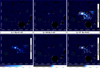 |
Fig. 4. Example of source injection. The model of diffuse emission between a pair of simulated galaxy clusters (masked within their R200; green dashed circles) found in the simulation with B0 = 0.1 nG (lower left panel) is multiplied by a factor fB = 1, 102, 104 imaged and masked after being injected into the source-subtracted sky visibilities (upper left, upper central, and upper right panels, respectively), or it is injected through the image-plane (lower centre and lower right panels for fB = 102 and 104, respectively). The image with fB = 1 in the upper left panel, due to the very low brightness of the model with B0 = 0.1 nG, is equal to the source-subtracted sky image Imempty, where the only features are the residuals from the source subtraction process that fall outside the masks. The white contours are set to 5 times the rms value in Imempty. |
The flux density was also multiplied by a constant factor fB ≡ [B0/(0.1 nG)]2. Under the assumption that the amplification of the magnetic field into the simulated filaments is affected by negligible small-scale dynamo (Ryu et al. 2008) and that it is thus mainly driven by the adiabatic compression of the magnetic field lines following from flux freezing4 into the plasma condensing during structure formation (Vazza et al. 2017), the magnetic field B in the simulation is scalable with respect to B0 and in turn the synchrotron emissivity is scalable with respect to  (assuming a constant ξe = 10−2).
2.5. Injection of model radio emission into real LOFAR images
The rescaled simulated image of each mock pair of galaxy clusters was injected into the source-subtracted measurement set (MS), following the procedure sketched in Fig. 1. In detail, a Fourier transform was performed on each rescaled image; the image was then written into the MS and finally added to the visibilities of the source-subtracted sky using WSCLEAN (Offringa et al. 2014). We note that this injection does not take into account direction-dependent effects that may act on the MS radio data. With the same software the resulting data set was imaged and deconvolved with a 20″ uv-taper and synthesised beam, and Briggs weighting scheme (Briggs 1995) with robust = −0.25 and 2000 minor cycles (see Fig. 4 for output examples). For realistic values of the normalisation parameter fB, the detectable emission is fragmented into small and sparse patches, associated with shocks internal to filaments. Therefore, we resort to statistical methods to assess the likelihood of each mock image to be compatible with our observed LOFAR fields. We compute the integral of the image power spectrum 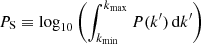 , where P(k′) is the power spectrum and kmin and kmax are determined by the image and beam size, respectively (see Fig. 9 for an example). The sky model subtraction can leave bright residual artefacts depending on the goodness of the model used. These residuals can be as bright as ∼0.1 Jy beam−1 around point-like sources and they may dominate the integral of the image power spectrum PS. A zero-padding mask was manually generated for each pair of clusters in order to exclude those artefact from the computation of PS in all images.
3. Results
From the cumulative probability distributions of the statistic PS resulting from all the source injections, we can assess how likely it is for a model to provide an expected value smaller than the one recovered from the observations. Using the image Imempty, a 2.5 deg × 2.5 deg square centred on the axis of the cluster pair, from which all the sources (point-like plus extended) have been subtracted, we compute  . The parameter
  corresponds to the total power in Imempty distributed over all scales from twice the beam size (kmin) up to half the image size (kmax). All images resulting from injection thus have PS equal to or larger than the value computed for Imempty (red dotted lines in Fig. 5). The statistic PS resulting from the image in which diffuse emission has not been subtracted Imdiffuse are indicated by the blue dashed vertical lines in Fig. 5. Totals of 6 and 15 mJy of diffuse emission have been found in Imdiffuse in excess of Imempty for RXC_J1659−J1702 and RXC_J1155−J1156, respectively. We outline the probabilities for the different models in Table 2, which also lists the results from the injection performed in the image plane found in general to produce different probabilities of non-detection with respect to injection through the uvw-plane. We discuss this alternative method in Sect. 4.
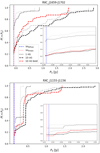 |
Fig. 5. Probability distributions of finding statistics PS smaller than the values set by the cluster pair RXC_J1659−J1702 (upper panel) and RXC_J1155−J1156 (lower panel) for scenarios with B0 as labelled. The vertical lines show the PS values computed without any injection from Imempty (red dotted) or Imdiffuse (blue dashed). The black and grey lines show results for source injection performed respectively in the visibility and image domains. The insets show a zoom-in on the bins where |
Probabilities of obtaining a statistic PS lower than the one observed in Imempty and Imdiffuse, computed from source injection performed in the uvw-plane and in the image-plane.
The overall probability of a magnetic field model is simply the product of the probabilities (of the model to produce lower statistics) of the two cluster pairs, since the experiments were run independently on each pair. We compute these probabilities in Table 2 (see ‘all’, bottom panel). A model is more likely to be discarded when its probability of having a smaller PS than in our LOFAR observations is either very small or very high.
Our main results can be summarised in the following way. The primordial scenario with a seed magnetic field of B0 ≃ 10 nG has a small probability P(< PS) ≃ 0.05 of explaining the small power excess in our observation of the RXC_J1659−J1702 and RXC_J1155−J1156 pairs, and we thus reject it with a confidence level (CL) of > 95%. The models with a lower seed magnetic fields B0 < 10 nG yield non-negligible probabilities (≥0.1) of producing a statistic equal to (or smaller than) the one observed. By tightening the constraints on individual cluster masses and on the presence of an inter-cluster filament connecting the clusters the model with B0 = 10 nG can be rejected with even higher confidence, CL > 97%. If any of the patches of diffuse emission observed is produced by shocks in the WHIM, then the B0 = 0.1 nG model is highly disfavoured as it is basically unable to produce any detectable emission (i.e. the probability in Table 2 that this model produces less diffuse emission than found in Imempty is always ≈1; these values are not plotted in Fig. 5). Although we do not reject this scenario, we consider it implausible (see Sect. 4).
4. Discussion
From the original simulation holding B0 = 0.1 nG, we extract the probability distribution functions (PDF) of the magnetic field values B10 Mpc across the mock filaments selected according to the properties of the observed cluster pairs. We plot the resulting PDF(log B10 Mpc) in Fig. 6. Given the expected lack of dynamo amplification in the WHIM, the magnetic field distributions PDF (log B10 Mpc) corresponding to the other B0 models can easily be rescaled linearly with the input seed field. We find a skewed distribution encompassing B10 Mpc = 1.0−7.4 nG values (90% confidence range) with median B10 Mpc = 2.5 nG (equivalent to log B10 Mpc = −8.6) for the full sample. We note that the value of the magnetic field that produces the simulated synchrotron emission is in the high part of the B10 Mpc distribution, as can be seen from the emission-weighted B10 Mpc distribution in Fig. 6. We also give in Fig. 7 the average profiles of mass-weighted magnetic field strength for all simulated filaments extracted with the procedure above, for the two cluster pairs. On average, the profile of magnetic field is very uniform across 10−20 Mpc, with an average magnetic field along the line of sight for these objects of ∼2−3 nG and a tail of rare and massive filaments that can reach ∼10 nG (Fig. 7). We find that the magnetic field along the direction connecting the clusters is enhanced with respect to the volume-filling values. The enhancement is significant regardless of whether the gas reaches temperatures typical of filaments (T > 105 K), but the enhancement is greater for higher temperatures, as expected from compression of the magnetic field lines during the structures growth (e.g. Gheller et al. 2016).
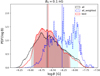 |
Fig. 6. PDFs of the log B10 Mpc field across all the simulated filaments in the B0 = 0.1 nG model, for all the pairs in the mock sample (black line) and for the best subsample (red line). The dashed blue lines show the log B10 Mpc distribution from all pairs weighted over the pixel emissivity. The filled hatched areas encompass the 10−90 percentile ranges. The vertical solid lines show the median of the distributions. |
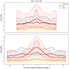 |
Fig. 7. Magnetic field profile along the cluster-to-cluster distance. Upper panel: average profile of mass-weighted magnetic field strength resulting from the B0 = 0.1 nG model for all inter-cluster filaments (black), extracted to resemble the cluster pair RXC_J1155−J1156; for the best subsample (red); and for a sample of images sampling an equal linear size (15 Mpc) extracted at random locations in the simulation (orange). The solid lines give the median values of the samples, while the filled areas encompass the 10−90th percentiles of the distributions. Lower panel: same plot, but for the mock sample extracted for RXC_J1659−J1702. |
To interpret the results provided in Fig. 5 and Table 2, we postulate three different assumptions that exploit the different types of source-subtraction performed in the analysis, which can be used to derive different priors from our data (vertical lines in Fig. 5):
-
I:
None of the residual diffuse emission after the point-like source subtraction (Imempty) is produced by the shocked cosmic web;
-
II:
All of the residual diffuse emission in excess of Imempty (i.e. Imdiffuse) is produced by the shocked cosmic web;
-
III:
At least some of the excess diffuse emission present in Imdiffuse comes from the cosmic web.
We analyse implications of the three assumptions separately in the following paragraphs.
4.1. Hypothesis I
Provided that we can fix the ξe acceleration efficiency at strong shocks (ξe ≈ 10−2), the assumption that none of the observed emission comes from cosmological shocks (I) produces, in principle, tighter constraints on B10 Mpc (and B0) since P(PS(Imempty)) ≤ P(PS(Imdiffuse)) always. In practice, the constraints are just slightly tighter due to the small amount of diffuse emission found in Imdiffuse with respect to Imempty. Thus, under the first hypothesis that we did not observe the cosmic web emission, by scaling the B10 Mpc distribution obtained from B0 = 0.1 nG to match the B0 = 10 nG model (i.e. a factor ×100) we infer an upper limit to the current median IGMF in filaments of B < 0.25 μG with 95% confidence (the same confidence level that applies to the rejection of B0 ≥ 10 nG models of the primordial magnetic field scenario). By considering the best subsample of cluster pairs with higher masses and connected by an inter-cluster filament, we can further improve the constraints on B by rejecting the B0 = 10 nG model with a higher CL > 97%.
Not all pairs of clusters are physically connected by a cosmic filaments, and in the absence of a detection in other wavelengths (via Sunyaev-Zeldovich or X-ray analysis; e.g. Govoni et al. 2019) one needs to resort to linking probabilities as a function of distance, which can be derived from cosmological simulations. For example, early dark matter-only simulations estimated that ∼80% of pairs in the same mass range as our clusters, and separated by ∼15 Mpc h−1, are physically connected by filaments (Colberg et al. 2005). With more recent and resolved simulations, also including gas physics, we can revise this number and tailor it to the exact mass difference and separation of our LOFAR pairs. Using the algorithm outlined in Banfi et al. (2021), we reconstructed the network of filaments connecting halos in our simulation by checking for the actual presence of a matter bridge between pairs of clusters with a 25 or a 15 Mpc separation. This allows us to associate a probability for the presence of a filament with each LOFAR observation, through the ratio of the number of physical filaments in the simulation (best sample) to the total pairs of galaxy clusters found at a given distance. This results in a 35% and 65% probability of having a filament between clusters at 25 and 15 Mpc separation, respectively. It should be noted that even in the case without an actual gas connection between clusters, the region in between is far from empty, because massive clusters at a relatively short separation are also indicators of a large cosmic overdensity, which is often associated with the presence of other filaments or threads of the cosmic web along the line of sight, which may account for a non-negligible radio emission. This still allows us to exclude B0 > 10 nG with high enough confidence. So, the absence of an actual filament does not dramatically affect the validity of the limits inferred from the full sample in this work.
4.2. Hypothesis II
The assumption that the excess diffuse emission present in Imdiffuse with respect to Imempty is entirely due to shocked plasma of the WHIM can be readily tested by looking in detail at the diffuse emission patches that have been detected. In Fig. 8 we present close-up clippings of the diffuse patches found close to the pair RXC_J1659−J1702, taken from the low-resolution LOFAR images (before source subtraction). They are meant to help in assessing the nature of some of the diffuse emission (dashed red circles in Fig. 8). We also give the position of sources already known from the VLA Faint Images of the Radio Sky at Twenty-centimeters (FIRST) survey (Becker et al. 1995). Most of the diffuse emission is plausibly linked to the lobes of radio-galaxies already detected at higher frequencies. Panel 7 shows what looks like either a radio lobe or an artefact linked to a low-frequency point source. Panels 2, 5, and 6 instead show diffuse emission that is not obviously linked to radio galaxies or to deconvolution artefacts. However, sources 5 and 6 are found (by looking at their coordinates) to be distant from the axis connecting the clusters, albeit within the imaged portion of the sky around the pair (see also Fig. 2). This makes their physical connection to the putative inter-cluster filament unlikely, even if the shocked cosmic web is expected to fill the space between the clusters in a non-trivial way, as shown in Fig. 3. Furthermore, the point-like source embedded in the diffuse emission in panel 6 is also found to be at a different redshift with respect to the cluster pair. For the above reasons, these patches can hardly be used in the comparison with the simulated inter-cluster filaments. The diffuse patches in panel 2 instead embed optical galaxies with redshift z = 0.087, 0.093, consistent with the cluster pair z = 0.095−0.101; however, they are likely dying faint radio lobes with no FIRST counterpart. Interestingly, the positions of Sloan Digital Sky Survey (SDSS) sources (orange plus signs) in the panels of Fig. 8 seem to cluster close to the diffuse radio emission. This trend is actually expected if the radio signal is caused by radio galaxies and lobes, which tend to be found in clusters or groups of galaxies (Prestage & Peacock 1988; Allington-Smith et al. 1993; Zirbel 1997; Wing & Blanton 2011). This behaviour additionally disfavours the link between the excess diffuse emission and the cosmic web. All in all, since there is no easy way to cross-check all the different patches, we still compute the statistics for the most conservative scenario by assuming that the level of observed diffuse emission in excess of Imempty is entirely due to the cosmic web. In this case the level of confidence associated with the rejection of the same models loosens. However, the models rejected by casting hypothesis II are the same ones resulting from hypothesis I, though at a slightly lower or even equal CL; for example, for the B0 = 10 nG best model the CL (for its rejection) decreases from 98% to 97%, while for the full sample it remains unchanged. Furthermore, since hypothesis II has already been falsified by the examples described above and shown in Fig. 8, the consensus for hypothesis I is strengthened, and we thus refer to it in order to draw our conclusions.
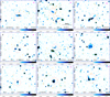 |
Fig. 8. Zoomed-in low-resolution sky images (20″, magenta solid circles) centred over the patches of diffuse emission found in Imdiffuse of RXC_J1659−J1702 (dashed red circles). The green crosses (×) show the position of FIRST sources. The orange plus signs (+) show the position of SDSS galaxies with known spectroscopic redshift. Panels are numbered from 1 to 9 going from left to right and top to bottom. 1″ = 1.84 kpc at z = 0.10; the 500 kpc scale is shown in panel 2 for comparison. The colour bars are in units of Jy beam−1. |
4.3. Hypothesis III
For completeness, we present an additional and interesting way of interpreting our data with respect to the simulation results, which is complementary to hypothesis I. We assume that at least some of the diffuse emission in excess of Imempty comes from the cosmic web. The associated probability is then trivially P(> PS) = 1 − P(< PS). In this case we are not interested in the level of diffuse emission in Imdiffuse since we want to produce at least the one in Imempty. This scenario, though disfavoured, cannot be discarded a priori since this would imply checking (e.g. through cross-correlations) all the different patches of diffuse emission in Imdiffuse and proving that all of them are not connected to the emission from the Cosmic Web; it is then instructive to inspect its implications. Under the assumption that we did see the cosmic web emission at least in part, then the B0 = 0.1 nG model is ruled out with high confidence (≥99%) since it is not able to produce any observable emission brighter than the noise level of our LOFAR observation. In this scenario B0 > 0.1 nG can be set as a lower limit to the primordial magnetic field intensity, and in turn B > 2 nG as the median value for the magnetic field into filaments today.
4.4. Visibility versus image plane injection
While checking that the source injection procedure (presented in Sect. 2 and sketched in Fig. 1) is actually needed in order to derive robust limits on B10 Mpc and B0 we also demonstrate that the method is essential to interpret observations in detail by means of the outcome of simulations when dealing with radio data. In this respect, we produced the same statistic PS for the simulations directly added to the residual image Imempty in terms of a simple image sum, rather than following the central FFT + write + sum procedure involving visibilities. This procedure is much simpler and faster (shortening the computing time by a factor of ∼600). In Fig. 9 we plot the power spectra resulting from the injection in the RXC_J1659−J1702 field of one source as an example (images of the same source are shown in Fig. 4) in order to inspect the differences between the injection through the uvw-plane (black lines) and the image-plane (grey lines) for the different B0 models. As can be seen by comparing the black and grey lines, when the injection is performed within the image-plane the level of simulated emission on large scales is generally underestimated. As a consequence the models are consistent with the data with different probabilities up to ±30%P(< PS) (see the values in Table 2). We interpret the difference in the results as being due to the lack of model convolution with the instrument’s point spread function (PSF). In addition, the lack of convolution of the emission with a visibility weighting scheme able to maximise the evidence for extended diffuse emission into the data may also play a similar role. As long as an upper cut on the scales of the emission (corresponding to a lower bound on the baseline length in radio interferometers) is taken into account, and detailed power spectrum information does not constitute the largest budget of uncertainty in one analysis (in our case it is the scatter in the properties of the unknown inter-cluster WHIM), the image sum is a much faster approach than the source injection through the uvw-plane; however, it should be used with caution as results are biased by a different sampling of the scales. The strength of the bias depends either on the sampling (window) function or the source power spectrum.
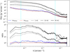 |
Fig. 9. Power spectrum of the injected filament shown in Fig. 4 for different B0 models, as labelled. The vertical cyan dotted lines show the integration scale limits used to compute PS. They correspond respectively to about half the largest scale in the image k−1 = 2173″ ∼ 483 pixels and k−1 = 40″ (corresponding to twice the synthesised beam full width at half maximum scale). The black lines show P(k) resulting from the source injection into uvw visibilities, whereas the grey lines show the result from the image-plane addition of the simulated image onto Imempty. Lower panel: same power spectra as in the upper panel, divided by the Imempty line. |
As a final caveat, our analysis assumes that for strong shocks in and around filaments, the acceleration efficiency of electrons is the one suggested by DSA (i.e. ξe ∼ 10−2). This assumes, in turn, that despite the rather low particle density and magnetisation, shocks can form and undergo particle acceleration similar to what is already observed for the outer regions of galaxy clusters in the form of giant radio relics (see van Weeren et al. 2019, for a review). Moreover, our analysis assumes that the acceleration of electrons at shocks can proceed independently on the obliquity between the upstream magnetic field and the shock normal. However, recent numerical works by Banfi et al. (2020) show that shocks surrounding the cosmic web are more often quasi-perpendicular than random chance, as an effect to the peculiar gas velocity flow following the formation of filaments. In this case the vast majority of shocks in filaments are quasi-perpendicular, and thus likely to be suitable for efficient electron acceleration (Xu et al. 2020). Furthermore, Masters et al. (2017) report a significant electron acceleration from the strong quasi-parallel shock while crossing the Saturn bow shock by the Cassini space mission (i.e. in plasma conditions similar to the intra-cluster medium). The acceleration seems to occur in the portion of the shock where upstream cosmic-ray streaming instabilities generate perpendicular small-scale magnetic field components, leading to particle acceleration.
5. Conclusions
In this work we attempted for the first time to combine dedicated LOFAR-HBA observations of inter-cluster filaments and numerical simulations of the magnetic cosmic web in order to derive upper limits on the magnetisation of the WHIM.
While our LOFAR observations do detect patches of diffuse emission of unclear origin, their morphology does not allow us to firmly associate the origin of the most prominent ones with the cosmic web. However, the presence of a faint diffuse large-scale excess in comparison with numerical models allows us to derive inferences on the average magnetisation of such filaments, and possibly on the allowed initial amplitude of primordial seed magnetic fields. As the main outcome of our work, by fixing ξe = 0.01 for strong shocks, we derive an upper limit for the median magnetic field strength in filaments connecting massive galaxy clusters: B10 Mpc < 0.25 μG. Based on the dynamical evolution of magnetic fields given by present simulations (which is mostly dominated by simple compression of magnetic field lines), this also implies an upper limit of B0 < 10 nG on the amplitude of primordial seed fields. The estimates above rely on the assumption that our observations constitute non-detections of diffuse emission from the cosmic web (hypothesis I).
As a mutually exclusive interpretation of our data, if some of the detected emission partially came from the shocked WHIM (hypothesis III), this would imply a median magnetic field of order of B10 Mpc ≥ nG (see e.g. Fig. 6). This would be an important outcome as it might also indicate primordial magnetic fields with intensity B0 ≥ 0.1 nG.
The hypothesis that all of the excess diffuse emission detected in our maps came from the cosmic web (hypothesis II) can be easily rejected even by a visual check of some of the sources. Given the uncertainties connected to our method and the limited statistics of the detections in our sample, we favour the first interpretation of our results (hypothesis I, setting B10 Mpc < 0.25 μG and B0 < 10 nG).
To compare our new limits with those of other recent works (Hackstein et al. 2016; Pshirkov et al. 2016; Vernstrom et al. 2017, 2019; Brown et al. 2017; O’Sullivan et al. 2020; Natwariya 2021, for a review, and Paoletti & Finelli 2019 for joint BICEP2/Keck – Planck 2018 updated results), we show them in Fig. 10 separating the limits inferred for the IGMF or the magnetic field intensity of the WHIM (red arrows) and for the primordial magnetic field intensity B0 (blue arrows). We note that our limits are still in agreement with the recent limits 0.134 < B0/nG < 0.316 set by the level of excess diffuse emission observed by the ARCADE2 and EDGES 21 cm line experiments (Natwariya 2021). Furthermore, an apparent tension seems to arise between our lower limit to B10 Mpc into filaments and the that derived from other probes such as the level of anisotropy in the arrival direction of charged ultra-high-energy cosmic rays used to limit the average amplitude of magnetic fields in voids to ≤1 nG (Hackstein et al. 2016), or from the non-detection of a trend of rotation measures from distant radio sources with respect to redshifts (Pshirkov et al. 2016). Although they are computed over similar linear scales (≥Mpc) and globally refer to the IGM, they can still hardly be directly compared since referred to different IGM environments (e.g. voids, filaments, averaged). Interestingly, a recent work suggests that primordial magnetic fields with amplitude ∼0.1 nG would possibly alleviate the existing tension between cosmological and standard candle-based estimates of H0 (Jedamzik & Pogosian 2020).
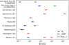 |
Fig. 10. Summary of the current upper and lower limits to the volume-averaged IGMF (red arrows), B in the filaments’ WHIM (green arrows), and B0 (blue arrows). |
While it is hard to derive conclusive limits from these data, as no robust detection (although tentative) of the diffuse emission from the cosmic web can be claimed, this first attempt highlights the potential of low-frequency radio observations in constraining extragalactic magnetic fields, and its relevance to the study of cosmic magnetogenesis. With the analysis and the values obtained in this work, we can forecast that we will produce tighter constraints than those posed by CMB experiments by covering a ∼ × 10 larger sample of cluster pairs similar to the ones analysed here, even in the case of other non-detections.
The magnetic flux through a closed loop C enclosing the surface S is simply ΦB = ∫SB ⋅ dS, valid for ideal plasma conditions.
Acknowledgments
We thank Klaus Dolag for providing corrections and helpful scientific feedback. NL and FV acknowledge financial support from the ERC Starting Grant “MAGCOW”, no. 714196. ABon acknowledges financial support from the ERC Starting Grant “DRANOEL”, no. 714245. ABot acknowledges support from the VIDI research programme with project number 639.042.729, which is financed by the Netherlands Organisation for Scientific Research (NWO). Radio imaging made use of WSClean v2.6 (Offringa et al. 2014) and DDF (Tasse et al. 2018). NL wishes to thank S. Carozzi and A. Crotti for psychological aid during and after the lock-down that followed the COVID-19 pandemic situation, when this work took shape. This paper is based (in part) on data obtained with the International LOFAR Telescope (obs. ID LC9_020, PI F.V.) and analysed using LOFAR-IT infrastructure. LOFAR (van Haarlem et al. 2013) is the Low Frequency Array designed, constructed by ASTRON and collectively operated by the ILT foundation. These data were (partly) processed by the LOFAR Two-Metre Sky Survey (LoTSS) team. This team made use of the LOFAR direction independent calibration pipeline (https://github.com/lofar-astron/prefactor) which was deployed by the LOFAR e-infragroup on the Dutch National Grid infrastructure with support of the SURF Co-operative through grants e-infra 160022 and e-infra 160152 (Mechev et al. 2017, PoS(ISGC2017)002). The cosmological simulations were performed with the ENZO code (http://enzo-project.org), which is the product of a collaborative effort of scientists at many universities and national laboratories. FV acknowledges the usage of computational resources on the Piz Daint supercomputer at CSCS-ETHZ (Lugano, Switzerland) under project s805, and he also acknowledges the usage of online storage tools kindly provided by the Inaf Astronomica Archive (IA2) initiave (http://www.ia2.inaf.it).
References
- Aghanim, N., Douspis, M., Hurier, G., et al. 2019, A&A, 632, A47 [NASA ADS] [CrossRef] [EDP Sciences] [Google Scholar]
- Akahori, T., Gaensler, B. M., & Ryu, D. 2014, ApJ, 790, 123 [NASA ADS] [CrossRef] [Google Scholar]
- Allington-Smith, J. R., Ellis, R., Zirbel, E. L., & Oemler, A., Jr. 1993, ApJ, 404, 521 [NASA ADS] [CrossRef] [Google Scholar]
- Banfi, S., Vazza, F., & Wittor, D. 2020, MNRAS, 496, 3648 [CrossRef] [Google Scholar]
- Banfi, S., Vazza, F., & Gheller, C. 2021, MNRAS, 503, 4016 [CrossRef] [Google Scholar]
- Becker, R. H., White, R. L., & Helfand, D. J. 1995, ApJ, 450, 559 [NASA ADS] [CrossRef] [Google Scholar]
- Beresnyak, A., & Miniati, F. 2016, ApJ, 817, 127 [NASA ADS] [CrossRef] [Google Scholar]
- Biffi, V., Planelles, S., Borgani, S., et al. 2018, MNRAS, 476, 2689 [NASA ADS] [CrossRef] [Google Scholar]
- Botteon, A., van Weeren, R. J., Brunetti, G., et al. 2020a, MNRAS, 499, L11 [Google Scholar]
- Botteon, A., Brunetti, G., Ryu, D., & Roh, S. 2020b, A&A, 634, A64 [NASA ADS] [CrossRef] [EDP Sciences] [Google Scholar]
- Briggs, D. S. 1995, Am. Astron. Soc. Meet. Abstr., 187, 112.02 [Google Scholar]
- Brown, S., Vernstrom, T., Carretti, E., et al. 2017, MNRAS, 468, 4246 [NASA ADS] [CrossRef] [Google Scholar]
- Brüggen, M., Ruszkowski, M., Simionescu, A., Hoeft, M., & Dalla Vecchia, C. 2005, ApJ, 631, L21 [NASA ADS] [CrossRef] [Google Scholar]
- Bryan, G. L., Norman, M. L., O’Shea, B. W., et al. 2014, ApJS, 211, 19 [NASA ADS] [CrossRef] [Google Scholar]
- Bykov, A. M., Vazza, F., Kropotina, J. A., Levenfish, K. P., & Paerels, F. B. S. 2019a, Space Sci. Rev., 215, 14 [CrossRef] [Google Scholar]
- Bykov, A. M., Petrov, A. E., Krassilchtchikov, A. M., et al. 2019b, ApJ, 876, L8 [CrossRef] [Google Scholar]
- Cen, R., & Ostriker, J. P. 1999, ApJ, 514, 1 [NASA ADS] [CrossRef] [Google Scholar]
- Colberg, J. M., Krughoff, K. S., & Connolly, A. J. 2005, MNRAS, 359, 272 [NASA ADS] [CrossRef] [Google Scholar]
- Davé, R., Cen, R., Ostriker, J. P., et al. 2001, ApJ, 552, 473 [NASA ADS] [CrossRef] [Google Scholar]
- Dedner, A., Kemm, F., Kröner, D., et al. 2002, J. Comput. Phys., 175, 645 [Google Scholar]
- de Gasperin, F., Dijkema, T. J., Drabent, A., et al. 2019, A&A, 622, A5 [NASA ADS] [CrossRef] [EDP Sciences] [Google Scholar]
- Dolag, K., Bartelmann, M., & Lesch, H. 1999, A&A, 348, 351 [NASA ADS] [Google Scholar]
- Donnert, J., Vazza, F., Brüggen, M., & ZuHone, J. 2018, Space Sci. Rev., 214, 122 [NASA ADS] [CrossRef] [Google Scholar]
- Gheller, C., & Vazza, F. 2019, MNRAS, 486, 981 [NASA ADS] [CrossRef] [Google Scholar]
- Gheller, C., Vazza, F., Brüggen, M., et al. 2016, MNRAS, 462, 448 [NASA ADS] [CrossRef] [Google Scholar]
- Gheller, C., Vazza, F., & Bonafede, A. 2018, MNRAS, 480, 3749 [CrossRef] [Google Scholar]
- Govoni, F., Orrù, E., Bonafede, A., et al. 2019, Science, 364, 981 [NASA ADS] [CrossRef] [Google Scholar]
- Hackstein, S., Vazza, F., Brüggen, M., Sigl, G., & Dundovic, A. 2016, MNRAS, 462, 3660 [CrossRef] [Google Scholar]
- Hoeft, M., & Brüggen, M. 2007, MNRAS, 375, 77 [NASA ADS] [CrossRef] [Google Scholar]
- Jedamzik, K., & Pogosian, L. 2020, Phys. Rev. Lett., 125, 181302 [CrossRef] [Google Scholar]
- Kang, H., Ryu, D., & Jones, T. W. 2012, ApJ, 756, 97 [Google Scholar]
- Locatelli, N., Vazza, F., & Domínguez-Fernández, P. 2018, Galaxies, 6, 128 [NASA ADS] [CrossRef] [Google Scholar]
- Macquart, J. P., Prochaska, J. X., McQuinn, M., et al. 2020, Nature, 581, 391 [CrossRef] [Google Scholar]
- Masters, A., Sulaiman, A. H., Stawarz, Ł., et al. 2017, ApJ, 843, 147 [CrossRef] [Google Scholar]
- Mechev, A., Oonk, J. B. R., Danezi, A., et al. 2017, Proceedings of the International Symposium on Grids and Clouds (ISGC) 2017, 2 [CrossRef] [Google Scholar]
- Mohan, N., & Rafferty, D. 2015, Astrophysics Source Code Library [record ascl:1502.007] [Google Scholar]
- Natwariya, P. K. 2021, Eur. Phys. J. C, 81, 394 [CrossRef] [EDP Sciences] [Google Scholar]
- Nicastro, F., Kaastra, J., Krongold, Y., et al. 2018, Nature, 558, 406 [NASA ADS] [CrossRef] [PubMed] [Google Scholar]
- Offringa, A. R., McKinley, B., Hurley-Walker, N., et al. 2014, MNRAS, 444, 606 [NASA ADS] [CrossRef] [Google Scholar]
- O’Sullivan, S. P., Brüggen, M., Vazza, F., et al. 2020, MNRAS, 495, 2607 [NASA ADS] [CrossRef] [Google Scholar]
- Paoletti, D., & Finelli, F. 2019, JCAP, 2019, 028 [CrossRef] [Google Scholar]
- Piffaretti, R., Arnaud, M., Pratt, G. W., Pointecouteau, E., & Melin, J. B. 2011, A&A, 534, A109 [NASA ADS] [CrossRef] [EDP Sciences] [Google Scholar]
- Prestage, R. M., & Peacock, J. A. 1988, MNRAS, 230, 131 [NASA ADS] [CrossRef] [Google Scholar]
- Pshirkov, M. S., Tinyakov, P. G., & Urban, F. R. 2016, Phys. Rev. Lett., 116, 191302 [NASA ADS] [CrossRef] [PubMed] [Google Scholar]
- Reiprich, T. H., Veronica, A., Pacaud, F., et al. 2021, A&A, 647, A2 [EDP Sciences] [Google Scholar]
- Ryu, D., Kang, H., Cho, J., & Das, S. 2008, Science, 320, 909 [NASA ADS] [CrossRef] [PubMed] [Google Scholar]
- Shimwell, T. W., Röttgering, H. J. A., Best, P. N., et al. 2017, A&A, 598, A104 [NASA ADS] [CrossRef] [EDP Sciences] [Google Scholar]
- Shimwell, T. W., Tasse, C., Hardcastle, M. J., et al. 2019, A&A, 622, A1 [NASA ADS] [CrossRef] [EDP Sciences] [Google Scholar]
- Smirnov, O. M., & Tasse, C. 2015, MNRAS, 449, 2668 [NASA ADS] [CrossRef] [Google Scholar]
- Stuardi, C., Bonafede, A., Wittor, D., et al. 2019, MNRAS, 489, 3905 [NASA ADS] [Google Scholar]
- Stuardi, C., O’Sullivan, S. P., Bonafede, A., et al. 2020, A&A, 638, A48 [EDP Sciences] [Google Scholar]
- Tanimura, H., Aghanim, N., Kolodzig, A., Douspis, M., & Malavasi, N. 2020, A&A, 643, L2 [EDP Sciences] [Google Scholar]
- Tasse, C. 2014a, ArXiv e-prints [arXiv:1410.8706] [Google Scholar]
- Tasse, C. 2014b, A&A, 566, A127 [NASA ADS] [CrossRef] [EDP Sciences] [Google Scholar]
- Tasse, C., Hugo, B., Mirmont, M., et al. 2018, A&A, 611, A87 [NASA ADS] [CrossRef] [EDP Sciences] [Google Scholar]
- Tasse, C., Shimwell, T., Hardcastle, M. J., et al. 2021, A&A, 648, A1 [EDP Sciences] [Google Scholar]
- Uchiyama, Y., Aharonian, F. A., Tanaka, T., Takahashi, T., & Maeda, Y. 2007, Nature, 449, 576 [NASA ADS] [CrossRef] [PubMed] [Google Scholar]
- Vacca, V., Oppermann, N., Enßlin, T., et al. 2016, A&A, 591, A13 [NASA ADS] [CrossRef] [EDP Sciences] [Google Scholar]
- van Haarlem, M. P., Wise, M. W., Gunst, A. W., et al. 2013, A&A, 556, A2 [NASA ADS] [CrossRef] [EDP Sciences] [Google Scholar]
- van Weeren, R. J., Williams, W. L., Hardcastle, M. J., et al. 2016, ApJS, 223, 2 [NASA ADS] [CrossRef] [Google Scholar]
- van Weeren, R. J., de Gasperin, F., Akamatsu, H., et al. 2019, Space Sci. Rev., 215, 16 [NASA ADS] [CrossRef] [Google Scholar]
- Vazza, F., Brüggen, M., Gheller, C., & Wang, P. 2014, MNRAS, 445, 3706 [NASA ADS] [CrossRef] [Google Scholar]
- Vazza, F., Ferrari, C., Brüggen, M., et al. 2015, A&A, 580, A119 [NASA ADS] [CrossRef] [EDP Sciences] [Google Scholar]
- Vazza, F., Brüggen, M., Gheller, C., et al. 2017, Classical Quantum Gravity, 34, 234001 [NASA ADS] [CrossRef] [Google Scholar]
- Vazza, F., Ettori, S., Roncarelli, M., et al. 2019, A&A, 627, A5 [NASA ADS] [CrossRef] [EDP Sciences] [Google Scholar]
- Vernstrom, T., Gaensler, B. M., Brown, S., Lenc, E., & Norris, R. P. 2017, MNRAS, 467, 4914 [NASA ADS] [CrossRef] [Google Scholar]
- Vernstrom, T., Gaensler, B. M., Rudnick, L., & Andernach, H. 2019, ApJ, 878, 92 [NASA ADS] [CrossRef] [Google Scholar]
- Vernstrom, T., Heald, G., Vazza, F., et al. 2021, MNRAS, 505, 4178 [CrossRef] [Google Scholar]
- Williams, W. L., van Weeren, R. J., Röttgering, H. J. A., et al. 2016, MNRAS, 460, 2385 [NASA ADS] [CrossRef] [Google Scholar]
- Wing, J. D., & Blanton, E. L. 2011, AJ, 141, 88 [NASA ADS] [CrossRef] [Google Scholar]
- Xu, R., Spitkovsky, A., & Caprioli, D. 2020, ApJ, 897, L41 [CrossRef] [Google Scholar]
- Zirbel, E. L. 1997, ApJ, 476, 489 [Google Scholar]
All Tables
Main parameters of the two pairs of galaxy clusters observed in this work, based on the Meta-Catalogue of X-ray Detected Clusters of Galaxies (MCXC; Piffaretti et al. 2011).
Probabilities of obtaining a statistic PS lower than the one observed in Imempty and Imdiffuse, computed from source injection performed in the uvw-plane and in the image-plane.
All Figures
|
Fig. 1. Diagram of the method outlined in Sect. 2. The thick boxes highlight the most computationally expensive steps. Links labelled ‘i’ are computed iteratively over the simulated pairs. |
| In the text | |
|
Fig. 2. LOFAR low-resolution (20″) images at 150 MHz of the cluster pairs RXC_J1659−J1702 (left panel) and RXC_J1155−J1156 (right panel). The dashed circles are centred on the clusters and have corresponding radius R500. Magnified images of the red dashed boxes in the left panel are shown in Fig. 8. The 5 Mpc unit at the redshift of the pairs z = 0.10, 0.14 is shown in the top right corner (left and right panels). The colour bars are in units of Jy beam−1. |
| In the text | |
|
Fig. 3. Example of mean gas temperature (top) and mock LOFAR-HBA observation (bottom, ν = 140 MHz, 25″ resolution, 250 μJy beam−1 noised added) from the ENZO simulation. The circles indicate the virial region of clusters; the magenta rectangles show the filaments. The detectable emission (≥3σ) is shown as green contours. The cluster field is placed at z = 0.1. |
| In the text | |
|
Fig. 4. Example of source injection. The model of diffuse emission between a pair of simulated galaxy clusters (masked within their R200; green dashed circles) found in the simulation with B0 = 0.1 nG (lower left panel) is multiplied by a factor fB = 1, 102, 104 imaged and masked after being injected into the source-subtracted sky visibilities (upper left, upper central, and upper right panels, respectively), or it is injected through the image-plane (lower centre and lower right panels for fB = 102 and 104, respectively). The image with fB = 1 in the upper left panel, due to the very low brightness of the model with B0 = 0.1 nG, is equal to the source-subtracted sky image Imempty, where the only features are the residuals from the source subtraction process that fall outside the masks. The white contours are set to 5 times the rms value in Imempty. |
| In the text | |
|
Fig. 5. Probability distributions of finding statistics PS smaller than the values set by the cluster pair RXC_J1659−J1702 (upper panel) and RXC_J1155−J1156 (lower panel) for scenarios with B0 as labelled. The vertical lines show the PS values computed without any injection from Imempty (red dotted) or Imdiffuse (blue dashed). The black and grey lines show results for source injection performed respectively in the visibility and image domains. The insets show a zoom-in on the bins where |
| In the text | |
|
Fig. 6. PDFs of the log B10 Mpc field across all the simulated filaments in the B0 = 0.1 nG model, for all the pairs in the mock sample (black line) and for the best subsample (red line). The dashed blue lines show the log B10 Mpc distribution from all pairs weighted over the pixel emissivity. The filled hatched areas encompass the 10−90 percentile ranges. The vertical solid lines show the median of the distributions. |
| In the text | |
|
Fig. 7. Magnetic field profile along the cluster-to-cluster distance. Upper panel: average profile of mass-weighted magnetic field strength resulting from the B0 = 0.1 nG model for all inter-cluster filaments (black), extracted to resemble the cluster pair RXC_J1155−J1156; for the best subsample (red); and for a sample of images sampling an equal linear size (15 Mpc) extracted at random locations in the simulation (orange). The solid lines give the median values of the samples, while the filled areas encompass the 10−90th percentiles of the distributions. Lower panel: same plot, but for the mock sample extracted for RXC_J1659−J1702. |
| In the text | |
|
Fig. 8. Zoomed-in low-resolution sky images (20″, magenta solid circles) centred over the patches of diffuse emission found in Imdiffuse of RXC_J1659−J1702 (dashed red circles). The green crosses (×) show the position of FIRST sources. The orange plus signs (+) show the position of SDSS galaxies with known spectroscopic redshift. Panels are numbered from 1 to 9 going from left to right and top to bottom. 1″ = 1.84 kpc at z = 0.10; the 500 kpc scale is shown in panel 2 for comparison. The colour bars are in units of Jy beam−1. |
| In the text | |
|
Fig. 9. Power spectrum of the injected filament shown in Fig. 4 for different B0 models, as labelled. The vertical cyan dotted lines show the integration scale limits used to compute PS. They correspond respectively to about half the largest scale in the image k−1 = 2173″ ∼ 483 pixels and k−1 = 40″ (corresponding to twice the synthesised beam full width at half maximum scale). The black lines show P(k) resulting from the source injection into uvw visibilities, whereas the grey lines show the result from the image-plane addition of the simulated image onto Imempty. Lower panel: same power spectra as in the upper panel, divided by the Imempty line. |
| In the text | |
|
Fig. 10. Summary of the current upper and lower limits to the volume-averaged IGMF (red arrows), B in the filaments’ WHIM (green arrows), and B0 (blue arrows). |
| In the text | |
Current usage metrics show cumulative count of Article Views (full-text article views including HTML views, PDF and ePub downloads, according to the available data) and Abstracts Views on Vision4Press platform.
Data correspond to usage on the plateform after 2015. The current usage metrics is available 48-96 hours after online publication and is updated daily on week days.
Initial download of the metrics may take a while.