| Issue |
A&A
Volume 652, August 2021
|
|
|---|---|---|
| Article Number | A144 | |
| Number of page(s) | 22 | |
| Section | Planets and planetary systems | |
| DOI | https://doi.org/10.1051/0004-6361/202040096 | |
| Published online | 25 August 2021 | |
Oort cloud Ecology
II. the chronology of the formation of the Oort cloud★
1
Leiden Observatory, Leiden University,
PO Box 9513,
2300 RA
Leiden,
The Netherlands
e-mail: spz@strw.leidenuniv.nl
2
Department of Physics and Astronomy, University of California,
Los Angeles,
CA
90095,
USA
Received:
9
December
2020
Accepted:
18
May
2021
Jan Hendrik Oort hypothesized the existence of a distant cloud of cometary objects that orbit the Sun based on a spike in the reciprocal orbital separation at 1∕a ≲ 10−4 au−1. The Oort cloud is the source of long-period comets, but has not been observed directly, and its origin remains theoretical. Theories on its origin evoke a sequence of events that have been tested individually but never as a consistent chronology. We present a chronology of the formation and early evolution of the Oort cloud, and test the sequence of events by simulating the formation process in subsequent amalgamated steps. These simulations start with the Solar System being born with planets and asteroids in a stellar cluster orbiting the Galactic center. Upon ejection from its birth environment, we continue to follow the evolution of the Solar System while it navigates the Galaxy as an isolated planetary system. We conclude that the range in semi-major axis between ~100 au and several ~103 au still bears the signatures of the Sun being born in a ≳1000 M⊙ pc−3 star cluster, and that most of the outer Oort cloud formed after the Solar System was ejected. The ejection of the Solar System, we argue, happened between ~20 Myr and 50 Myr after its birth. Trailing and leading trails of asteroids and comets along the Sun’s orbit in the Galactic potential are the by-product of the formation of the Oort cloud. These arms are composed of material that became unbound from the Solar System when the Oort cloud formed. Today, the bulk of the material in the Oort cloud (~70%) originates from the region in the circumstellar disk that was located between ~15 au and ~35 au, near the current location of the ice giants and the Centaur family of asteroids. According to our simulations, this population is eradicated if the ice-giant planets are born in orbital resonance. Planet migration or chaotic orbital reorganization occurring while the Solar System is still a cluster member is, according to our model, inconsistent with the presence of the Oort cloud. About half the inner Oort cloud, between 100 and 104 au, and a quarter of the material in the outer Oort cloud, ≳104 au, could be non-native to the Solar System but was captured from free-floating debris in the cluster or from the circumstellar disks of other stars in the birth cluster. Characterizing this population will help us to reconstruct the history of the Solar System.
Key words: methods: numerical / Oort Cloud / comets: general / Sun: general
The source code, input files, and simulation data for this manuscript are available at 10.6084/m9.figshare.13214471. A tutorial on how to run the various codes in AMUSE is available at https://github.com/spzwart/AMUSE-Tutorial.
© ESO 2021
1 Introduction
The formation of the Oort cloud (Oort 1950) requires a sequence of events on temporal and spatial scales that span more than eight orders of magnitude, from the Solar System (on scales of years and au) to the entire Galaxy (on scales of Gyr and kpc). As a consequence, the formation of the Oort cloud was not a simple happening; Occam’s razor does not seem to apply here.
Individual events that led to the formation of the Oort cloud have in the past been modeled separately to explain specific features (see e.g., Hayashi et al. 1985; Dones et al. 2004a, 2015; Higuchi et al. 2007; Lykawka & Mukai 2008; Leto et al. 2008; Paulech et al. 2010; Rickman 2014; Fouchard et al. 2018). However, the chain of events has never been tested as a causal sequence. We present the results of computer simulations designed to model the chronology of the formation of the Oort cloud in which individual processes are included at their proper scales. Each phase is simulated precisely and is connected to the subsequent phase of the cascade. By doing so, we construct a consistent picture of the formation and early evolution of the Oort cloud.
In our analysis, we assume that the Solar System formed, like most stars (Lada & Lada 2003; Adams 2010), in a giant molecular cloud in which gas contracts under its own gravity, and stars form with disks around them (Beckwith et al. 1990; McKee & Ostriker 2007; Gavagnin et al. 2017). The Solar System then probably formed in a cluster of stars which interacted mutually before the Sun escaped the cluster (Portegies Zwart et al. 2009). The circumstellar disk, a leftover from the star-formation process, led to the coagulation of planets (Kokubo & Ida 1998, 2002; Kenyon & Bromley 2006; Wyatt 2008; Levison et al. 2010b; Williams & Cieza 2011; Emsenhuber et al. 2021, 2020; Schlecker et al. 2021) and a large number of planetesimals (Johansen et al. 2007, 2021; Johansen & Lambrechts 2017; Popovas et al. 2018)1. The presence of nearby stars in the parent cluster will have affected the morphology of the gaseous disk through tidal perturbations (Clarke & Pringle 1993; Pfalzner et al. 2005; Winter et al. 2018; Cuello et al. 2019), photo-evaporation (Johnstone et al. 1998; Adams et al. 2004; Clarke 2007), and stellar winds (Offner & Arce 2015).
The evolution of the circumstellar disk has profound consequences for the orbits of the newly formed planets (Laughlin & Adams 1998; Breslau et al. 2014; Vincke et al. 2015; Vincke & Pfalzner 2016; Concha-Ramírez et al. 2021), although it is currently difficult to quantify these effects. The formation of the Oort cloud, however, seems somewhat problematic in this picture (but see Levison et al. 2010a; Vokrouhlický et al. 2019, for a counter argument). We argue that the majority of the Oort cloud formed after the Sun escaped the cluster because perturbations of nearby stars would easily ionize an earlier Oort cloud (see also Higuchi & Kokubo 2015).
In the present paper, we present a study of the formation of the Oort cloud from a numerical perspective. The chain of events that lead to the Oort cloud can now be simulated in its entirety, although not fully self-consistently. We revisit this problem because we feel slightly overwhelmed by the enormity of the literature and the changing paradigm over the years. We hope to contribute to a clearer picture of the processes that appear to be relevant to the formation and evolution of the Oort cloud.
We perform a numerical investigation and show that the Oort cloud was not formed in any straightforward manner, but resulted from a complex interplay during the Sun’s infancy between the Sun itself and the neighboring stars, free-floating debris, the Galactictidal field, and planetary scattering. Each of these components turn out to be important, although their relative contributions are sometimes hard to quantify. The lack of a simple formation mechanism, and a conspiracy of processes instead, make the Oort cloud unique. A complicated story requires a complicated numerical approach that covers many time and size scales. Apart from stellar evolution in the early star-cluster phase, the physics is relatively simple. We deal with the fundamentally chaotic nature of the underlying physics (see Miller 1964; Goodman et al. 1993)by repeating calculations with a different random seed. In this discussion, we limit ourselves mainly to Newtonian physics (Newton 1687). We address each component of this calculation separately but knit the results together to from a homogeneous narrative on the formation and evolution of the Oort cloud as part of the Solar System.
The timescale of Oort-cloud formation is probably closely connected to the birth environment of the Solar System (Brasser et al. 2012). If born in a star cluster, as argued by Portegies Zwart (2009); Adams (2010); Parker (2020); Pfalzner & Vincke (2020), with a characteristic size of ~1 pc and with ~2500 siblings (Portegies Zwart 2019), asteroids in wide and highly elliptic orbits are vulnerable to being stripped from the Solar System by the cluster potential or by passing stars (see also Nordlander et al. 2017). Pfalzner & Vincke (2020) on the other hand, derive an even higher density cluster with a density of up to ~ 105 M⊙ pc−3. If formed too early in the lifetime of the Solar System, the outer parts of the Oort would be lost due to stripping when a small change in relative velocity  is induced upon the asteroids (see Fig. 1). So long as the Sun is a cluster member, asteroids with an eccentricity of e ≳ 0.98 with a semi-major axis of a ≳ 2400 au (a(1 − e) ≳ 50 au) are easily lost.
In the following section, we discuss our current understanding of the outer Solar System. We then describe the numerical setup and its ingredients in Sect. 3. In Sect. 4.1, we discuss the simulation results, and describe a holistic viewof the evolution of the Sun and proto-Oort cloud in the Galaxy in Sect. 4.2.1. The consequences of resonant planetary orbits are discussed in Sect. 4.2.2. These arguments are supported by simulations presented in Table 1. To further explore the consequences of alternative models on the formation of the Solar System, we include calculations adopting planetary orbits in resonance. We conclude in Sect. 5.
2 Current understanding of the outer Solar System
We summarize our current understanding of the remote parts of the Solar System, starting with the Kuiper-belt region, and subsequently move on to the outer parts.
Four regimes in the outer parts of the Solar System are important for this discussion, including: the dynamical class of trans-Neptunian objects (TNOs), theparking zone2, the Hills cloud, and the Oort cloud (for a review see Malhotra 2019). The inner three regions could have been populated and affected by encountering stars before the Sun escaped the cluster. In that case, the presence and orbital distribution of asteroids in the parking zone and Hills cloud could provide interesting constraints on the dynamical evolution of the Sun in its birth cluster before it was ejected (see also Moore et al. 2020).
2.1 The trans-Neptunian region and Kuiper belt
The phase-space structure in the Edgeworth-Kuiper belt is complex (Edgeworth 1943; Kuiper 1951). Close to the perturbing influence of Neptune (the red curve in Fig. 1 marks the outer boundary of the conveyor belt3; see the dotted line in Fig. 2) we find multiple families of Kuiper-belt objects. The most striking might be the scattered disk (Brown 2001; Luu & Jewitt 2002; Trujillo et al. 2000; Nesvorný 2020), but there are other exotic orbital characteristics observed in this region, including the warp (at an inclination of  ; Volk & Malhotra 2017), the mix of resonant families (Chiang et al. 2003), the broad distribution in eccentricity and inclination of the Plutinos (Malhotra 1993; Brown 2001), the orbital topology of the classical belt population (Elliot et al. 2005), the outer edge at the 1:2 mean-motion resonance with Neptune (Gomes et al. 2004), and the extent of the scattered disk (Gladman et al. 2001). Apart from perhaps the population of almost circular objects in the classical Kuiper belt (Tegler & Romanishin 2000), many of these characteristics can be explained at least qualitatively with some incarnation of the Nice model (Gomes et al. 2005; Morbidelli et al. 2005; Tsiganis et al. 2005; Levison et al. 2008, see Sect. 2.5 for more on the Nice model). Some of these features in the Kuiper belt originated ≳ 50 Myr after the planets formed (Nesvorný 2020).
Here we demonstrate that it is possible to reconstruct part of the history of the Solar System from the kinematics and phase-space distribution of the orbiting bodies (see also Moore et al. 2020). Although we consider the Edgeworth-Kuiper belt to be crucial to our understanding of the formation and early evolution of the Solar System, the present paper focuses on the Oort cloud and its formation.
2.2 Sedna, other trans-Neptunian objects in the parking zone, and the Hills cloud
To date, several asteroids have been observed beyond the Kuiper cliff (at ~ 48 au), between a few hundred and a few thousand astronomical units (au) with a pericenter distance of ≳ 50 au (Sheppard et al. 2019; Alexandersen et al. 2019). These include the dwarf planet 90377 Sedna (Brown et al. 2004), 2012 VP113 (Sheppard et al. 2014), and a dozen others. These objects can be divided into two clusters, one population with their argument of pericenter at ~310° (Trujillo & Sheppard 2014), and another at the opposite side (Sheppard et al. 2019). This small number of known detached trans-Neptunian objects can, in part, be attributed to observational selection effects because they are far (Alexandersen et al. 2019), red (Brucker et al. 2009), and tend to have a relatively small albedo (Rabinowitz et al. 2006).
Also from the outer regions of the Solar System, the area in phase space where Sedna and family are found is hard to reach, meaning that the asteroids in this region cannot have come from either direction, the inner Solar System or the periphery. This unreachable area in parameter space is called the parking zone (Jílková et al. 2015), and is identified as such in Fig. 1. Asteroids in this region keep their orbital parameters for a very long time, possibly even as long as the age of the Solar System. We note that, if the asteroids in the parking zone cannot have come from the inner Solar System, and they do not have an origin from the periphery, they either formed in situ or were injected there by other means. The several observed dwarf planets and asteroids (such as Sedna) in this region preserve evidence for the dynamical history of the Solar System (Kaib & Quinn 2008; Jílková et al. 2015) and can be used to constrain its origin.
These arguments led to the hypothesis that Sedna and family were captured from another star in the parent cluster (Jílková et al. 2015). In this case, Sedna and family would have been captured from the circumstellar debris disk around another star. The population of asteroids in the parking zone may then form the leftover evidence for such a captured population (Nurmi et al. 2002; Morbidelli & Levison 2004; Shankman et al. 2011; Napier et al. 2021a).
Such a capture then must have happened more than 4 Gyr ago, and in that time frame the influence of the ice-giant planets would have caused the orbits of Sedna and family to change, in particular their arguments of pericenter should have randomized. But their orbits are such that they pass the pericenter at the same side of the Sun (Trujillo & Sheppard 2014).
Based on the alignment of the arguments of pericenter of the Sedna family of objects, Batygin & Brown (2016) and Batygin et al. (2019) argued in favor of the existence of a planet in the inner Oort cloud. Such a planet in a wide orbit or possibly even a stellar companion to the Sun could induce orbital characteristics similar to those observed in Sedna and other detached trans-Neptunian objects (Nesvorný 2020), or even affect the orbits of asteroids in the parking zone (Madigan & McCourt 2016; Zderic & Madigan 2020).
The main motivation for an extra planet disappeared, as the alignment of the arguments of pericenter turn out to be an observational selection effect (Sheppard et al. 2019; Napier et al. 2021b). Although a binary companion is currently probably absent (Melott & Bambach 2010; Hills 1984; Hut 1984), the Sun might have had one in the past (Siraj & Loeb 2020), particularly because such wide stellar companions are rather common among other stars (Kaib et al. 2013).
Further out, we find the hypothetical Hills cloud (Hills 1981) between the outer edge of the parking zone (≳ 1000 au) and the inner edge of the Oort cloud (≲20 000 au). The origin of the objects in the Hills cloud is unclear, but the population could be related to trans-Neptunian objects (Fernandez & Ip 1981; Dones et al. 2015). Hills (1981) estimated the total mass to exceed that of the Oort cloud by as much as a factor of 100 (see however Dones et al. 2000, who argue in favor for comparable populations). The majority of trans-Neptunian objects have prograde orbits (Kavelaars et al. 2020) and isotropic distributions in mean anomaly, longitude of the ascending node, and the argument of perihelion (Bernardinelli et al. 2020). These support an inner Solar System origin because asteroids scattered from the circumstellar disk tend to have prograde orbits (Moore et al. 2020), whereas the orbits of captured asteroids may well be retrograde, depending on the encounter that introduced them into the Solar System (see also Hanse et al. 2018; Napier et al. 2021a). The dynamical history of the Solar System in its birth cluster therefore plays an important role in the formation and orbital topology of asteroids in the parking zone and the Hills sphere (Parker 2020). Because of a lack of perturbing influences, signatures of a captured population in the parking zone remain noticeable for much longer than in other parts of the Solar System.
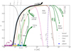 |
Fig. 1 Orbital migration of asteroids and how they end-up in the Oort cloud. Several of the thin curves are also plotted in Fig. 3. The four major planets are indicated with their current semi-major axis and eccentricity as blue dots. The initial circumstellar disk is presented in five colors, depending on the final destination of the asteroids populating the different disk sections. The arrows indicate the movement of asteroids originating from the disk or captured from other stars. The timescales presented near the arrows give an estimate of the timescale of migration. The colors indicated in the legend give the original inner disk (magenta), which mainly migrates away from resonant orbits (Delbo’ et al. 2017) (four important resonances are indicated with thin vertical dotted lines). Ochre indicates those asteroids that are ejected from the Solar System on a relatively short timescale (≲ 10 Myr). Light blue indicates the kernel and the resonant Kuiper belt. The light green and dark green curves show the migration patterns of the asteroids that eventually reach the Oort cloud. These objects migrate from a semi-major axis of a few tens of au to beyond 104 au through a narrow neck of high eccentricity. The asteroids in the dark green area require external support from a stellar encounter to be able to migrate to the Oort cloud. This migration is more visible in Fig. 3, where the eccentricity (y-axis) is in logarithmic units. We note that the closer an asteroid is to the Hill radius (vertical red dotted line to the right), the quicker its orbit will be circularized by the Galactic tidal field (see also Fig. 7, where this is illustrated). The gray, pink, and brown curves indicate where the relative velocity kick imparted at apocenter by the Galactic tidal field to an asteroid is δv = 10−8, 10−5, and 10−3 of the orbital velocity, respectively. The purple dashed curve indicates the orbital separation and eccentricity for which the tidal eccentricity damping timescale is equal to the orbital period (see Duncan et al. 1987). |
Simulations of the young Solar System.
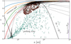 |
Fig. 2 Orbital distribution of the scattered (green dots) and captured (brown) asteroids. These conditions originate from the scatter and capture calculations, but form the initial conditions for subsequent calculations. The former are scattered from the circumstellar debris disk by a close encounter with another star in the parent cluster. The latter population is captured from another star with which the Sun interacted in its parent cluster. The simulations for both populations are described inTable 2. The small thin black lines from each dot-point point in the direction in which the orbit migrates over 300 Myr (we adopted 300 Myr here for the presentation, although we realize that adopting 100 Myr would have been a more systematic choice). These data were acquired by integrating the Solar System in the tidal field of the Galaxy. The asteroids that orbit the outer and inner parking zones are hardly affected by the Galactic tidal field. Those near the conveyor belt are strongly affected by the giant planets and some eventually reach the Oort cloud. The thin black dotted curve is parallel to the 2.5 Hill-radii to the right of Neptune’s pericenter influence (solid red curve), and indicates the extent to which the planet still affects the orbits of the asteroid. Simulation parameters are listed in Table 2. |
2.3 The Oort cloud
Discussions over the Öpik-Oort cloud began in 1932 by Öpik (Öpik 1932) who discussed the origin of nearby parabolic orbits in the Solar System, and in 1950 by Oort (Oort 1950) with the discovery of a spike in the reciprocal orbital separation 1∕a ≲ 10−4 au−1 of observed comets. Oort (1950) argued that the long-period comets originated from a region between 25 000 au and 200 000 au from the Sun. Today, these estimates have not changed considerably (Correa-Otto & Calandra 2019).
The outer limit is considered to coincide with the Hill radius (Hill 1913) of the Sun in the Galactic potential (Chebotarev 1965). The origin and precise location of the inner edge are less clear (Hills 1981; Leto et al. 2008) and are still debated (Brasser & Schwamb 2015). What defines the transition region between the Hills cloud and the Oort cloud also remains unclear.
The mass of the Oort cloud is estimated to range from 1.9M⊕ (Weissman 1996) to 38M⊕ (Weissman 1983). These estimates seem somewhat on the high side when compared to those based on numerical simulations, which arrive at 0.75 ± 0.25M⊕ (Brasser 2008) to 1.0 ± 0.4 M⊕ (Fernández & Brunini 2000).
With a typical comet-mass of a few times 1012 to 1014 kg (Rickman et al. 1987; Sosa & Fernández 2009, 2011) the Oort cloud contains  comet-sized objects. Interestingly, this estimate is comparable to Oort’s original estimate of ~ 1011 objects (Oort 1950), and to the density of interstellar asteroids (Engelhardt et al. 2017; Portegies Zwart et al. 2018; ’Oumuamua ISSI Team 2019; Pfalzner et al. 2020).
2.4 The formation and early evolution of the outer Solar System
Estimates of the formation timescale of the Oort cloud range from instantaneously after the formation of the Sun (Fernández 1997), synchronously with Jupiter’s formation (Stevenson & Lunine 1988; Fernández & Brunini 2000; Dones et al. 2004b), to after Jupiter formed and potentially migrated (Shannon et al. 2019), to slow growth over several 100 Myr (Kaib & Quinn 2008; Nordlander et al. 2017), and even to gigayear timescales (Duncan et al. 1987).
Two main scenarios are popular for the formation of the Oort cloud: one stipulates that the cloud formed mainly by ejecting inner Solar System material through planet–disk interactions (Dones et al. 2000, 2004a), and the other concerns formation through two distinct processes: Local disk asteroids are ejected into an inner region at 3000–20 000 au, while the outer region at ≳20 000 au is mainly accreted from free-floating debris in the parent star cluster (Zheng et al. 1990; Valtonen et al. 1992; Brasser et al. 2006, 2007; Brasser 2008; Levison et al. 2010a). Planets could also be captured in this way (Perets & Kouwenhoven 2012), possibly explaining the origin of a hypothetical exoplanet in the outer parts of the Solar System (Mustill et al. 2016).
The relatively low mass in some of the numerically derived estimates stem from the low efficiency, which ranges from ~ 1.1% (Leto et al. 2008; Morbidelli et al. 2009), ~2% (Correa-Otto & Calandra 2019) to ~4% (Brasser et al. 2010), at which point disk material is launched into a bound Oort cloud (Paulech et al. 2010); the majority of objects are expected to escape the Solar System or hit the Sun. The giant planets could therefore be insufficiently efficient to explain the currently anticipated mass of the Oort cloud (Brasser et al. 2006, 2012; Kaib & Quinn 2008).
If the entire Oort cloud originates from the depletion of asteroids between Uranus and Neptune (see also Fouchard et al. 2013), this region must have been populated by objects with a total mass of 100 to 3800 MEarth (Fouchard et al. 2014a,b). In a disk with a density profile of ρ ∝ r−1.5 between 0.1 au and 45 au, about half the mass is between the orbits of the ice giants. To supply the Oort cloud with sufficient material, the proto-planetary disk must then have had a mass of 200 to 7600M⊕ (or equivalently ~0.001 to 0.02 M⊙) in comet-sized asteroids, which is consistent with other estimates (Crida 2009).
Given the low efficiency of the ice-giants to produce the Oort cloud, more than 90% is likely to have come from elsewhere; such as the circumstellar disks of other stars (Levison et al. 2010a), free-floating debris in the parent cluster (Zheng et al. 1990; Neslušan 2000), the capture of interstellar objects (Valtonen & Innanen 1982; Hands & Dehnen 2020; Pfalzner et al. 2021), or accretion from the circumstellar disks of other stars (Fernández & Brunini 2000; Levison et al. 2010a).
The orbits of captured asteroids could be rather distinct from those produced by scattered asteroids from the proto-planetary disk (Hands et al. 2019; Higuchi & Kokubo 2020). In the Oort cloud, both populations will be affected by the Galactic tidal field (Duncan et al. 1987; Fouchard et al. 2006b) and probably mix on a timescale of a few hundred million years. Orbital inclinations isotropize on this timescale, and eccentricities thermalize (Fouchard et al. 2006a; Higuchi & Kokubo 2015).
Once fully developed, the Oort cloud erodes by injecting comets into the inner Solar System through Kaib-Quinn jumpers (Kaib & Quinn 2008) or by a more gradual process (sometimes referred to as creepers; Fouchard et al. 2014a, 2018), but also because of encounters with molecular clouds (Duncan et al. 2011) and tidal interaction with the Galaxy (Heisler & Tremaine 1986; Levison et al. 2001; Gardner et al. 2011; Torres et al. 2019). These external perturbations may be the main reason why comets are launched from the Oort cloud into the inner Solar System. This process was suggested to lead to periodic showers of comets (Davis et al. 1984; Gardner et al. 2011) causing mass extinctions every ~ 29.7 Myr (Raup & Sepkoski 1984; Rampino & Prokoph 2020). However, the wide companion to the sun implied by these periodic showers was never found (Luhman 2014), and re-analysis of the data shows that there is no statistically significant evidence for a periodicity in these mass extinctions (Patterson & Smith 1987; Jetsu & Pelt 2000; Bailer-Jones 2009).
2.5 The Nice model
Many of the model simulations above depend on some sort of chaotic reorganization in the early Solar System. This could have happened during or shortly after the formation of Jupiter (Li et al. 2006) up to about half a gigayear after the planets formed (Neslušan et al. 2009; Leto et al. 2009). This chaotic reorganization was introduced to explain the enhanced flux of asteroids throughout the young Solar System (Morbidelli et al. 2005; Tsiganis et al. 2005; Gomes et al. 2005), which could have led to a peak in the flux of lunar impactors (late-heavy bombardment is a commonly used term; Hartmann 1965, 1966; Alvarez & Muller 1984; Stöffler & Ryder 2001; Neukum et al. 2001; Ryder 2002).
Follow-up analyses indicated that the impact period could be between 4.2 and 3.5 Gyr ago (Fritz et al. 2014; Zellner 2017; Bottke & Norman 2017), rather than being a peak, rendering the need for a disturbance in the force in the early Solar System unnecessary. Re-analysis of the lunar impact statistics by Lineweaver (2010) indicated that a high flux of impactors is not needed to explain the lunar cratering record. This study was further supported by the re-analysis of the 267 Apollo samples on 40Ar/39Ar isotope ratios, where it was demonstrated that the material on the moon arrived in a continuously decreasing flux rather than a peak (Boehnke & Harrison 2016, 2018).
The Nice model is successful in explaining several aspects of the Solar System, including the orbital topology of the giant planets (Morbidelli et al. 2007), the obliquity of Uranus (Wong et al. 2019), Trojan asteroids (Emery et al. 2015), irregular moons (Bottke et al. 2010), some morphologies of the Kuiper belt (Morbidelli & Nesvorný 2020), and several other curious orbital choreographies (Levison et al. 2008; Shannon et al. 2019). Although, the Nice model seems to fail in explaining the global structure of the Oort cloud (Fouchard et al. 2018, but see also Shannon et al. 2019, for competing arguments based on the rocky comet C/2014 S3 (PANSTARRS)), it might be hard to find a single alternative model that can explain so many phenomena in the Solar System. One aspect of the Nice model that may be important for explaining the phenomena of the Solar System is a period in which the orbits tend to change chaotically (Thommes et al. 2008). Such a chaotic phase can be initiated by planetary resonance – as in the Nice model – induced by a passing star or by the last phase of evaporation of the circumstellar disk.
Several independently developed explanations exist, including models based on internal dynamical processes (Duncan et al. 1995; Ida et al. 2000), encounters with other stars (Ida et al. 2000; Kobayashi et al. 2005; Torres et al. 2019), or a small molecular cloudlet in a wide orbit around the Sun (Emel’yanenko 2020). However, there is no global model that explains the Solar System in unison.
This early phase in the evolution of the Solar System appears far from being understood from first principles, and more research on this topic would help to understand the apparent stability and inertness of the current Solar System.
Simulations of the Solar System with captured and scattered asteroids in the Galactic potential.
3 Methods, models, and simulations
This section explains the numerical methods, the initial conditions, and simulations that we used to qualify and quantify theformation and early evolution of the Oort cloud. Our calculations are not self-consistent because the results were not produced in a single simulation, but the results are melded together to form a consistent understanding.
We start with a discussion on the software framework, the Astrophysics Multipurpose Software Environment (AMUSE; see Sect. 3.1), which was used for the simulations presented here. We discuss each of the following processes:
- A.
The evolution of the circumstellar disk of an isolated Solar System (see Sect. 3.2 and Table 2).
The calculation includes the four giant planets orbiting the Sun together with a disk of mass-less particles. The entire setting is integrated in the potential of the Galaxy, starting with the approximate position in the Galaxy where the Sun was 1 Gyr ago, and lasts for 1 Gyr.
- B.
The evolution of the Solar System in its birth cluster (Sect. 3.3 and Table 3).
The arguments here are based on two quite distinct calculations: first a simulation of 2000 stars in a virialized cluster with a half-mass radius of ~1 pc. We study the evolution of debris disks under the influence of the encounters with neighboring stars. In a second calculation, we study the exchange efficiency and orbital characteristics of the circumstellar disks that were perturbed in encounters between two stars. These two simulations are used to understand the orbital parameters of various populations of asteroids:
- C.
Transport of asteroids along the conveyor belt and eccentricity damping by the tidal field once the Oort cloud is reached (see Sect. 3.4 and Table 4).
The formation of the Oort cloud is supported by simulations of the population of asteroids in the conveyor-belt region. These calculations include the four giant planets (with various orbital configurations) and the Galaxy’s tidal field. Both are necessary to study the transport of asteroids from the planetary region to the Oort cloud. The eccentricity and semi-major axis of the asteroids increases when evolving along the conveyor belt. This process is driven by the major planets. Once the pericenter of the orbits of the asteroid detaches from the major planets, the Galactic tidal field dampens the eccentricity of the orbits.
Figure 1 presents a schematic overview of the evolution of the Oort cloud. Asteroids near Jupiter and Saturn are vulnerable to being ejected on a relatively short timescale (≲ 10 Myr), whereas asteroids originally formed between Uranus and Neptune, and the scattered and captured populations (green arrows), tend to reach the Oort cloud on a much longer timescale of ~ 100 Myr. All asteroids that eventually reach the Oort cloud pass through the narrow neck at an eccentricity of ≳ 0.998 at a semi-major axis of around 104 au, after which they are subjected to eccentricity damping by interacting with the Galactic tidal field (green arrows to the right in Fig. 1). Figure 3 presents a superposition of simulation data ~100 Myr after the Solar System escaped its birth star cluster. This data originates from multiple calculations that simulate various aspects of the formation of the Oort cloud.
Simulation of the Solar System with asteroids in the conveyor belt.
3.1 The Astrophysics Multipurpose Software Environment
The calculations in this study are performed using the Astrophysics Multipurpose Software Environment (Portegies Zwart & McMillan 2018). AMUSE is a modular language-independent framework for homogeneously interconnecting a wide variety of astrophysical simulation codes. It is built on public community codes that solve gravitational dynamics, hydrodynamics, stellar evolution, and radiative transport using scripts that do not require recompilation. The framework adopts Noah’s Arc philosophy, meaning that it has incorporated at least two codes that solve the same physics (Portegies Zwart et al. 2009).
Most calculations are carried out using a combination of symplectic, direct, N-body test-particle integration and the tidal field of the Galaxy. For the former two, we use Huayno, which adopts the recursive Hamiltonian splitting strategy (much like bridge; see Fujii et al. 2007; Portegies Zwart et al. 2020) to generate a symplectic integrator that conserves momentum to machine precision (down to 10−14 in normalized units; Pelupessy et al. 2012). Additional calculations were performed using the ABIE code (Roa 2020), NBODY6++GPU (Wang et al. 2015), and REBOUND (Rein & Liu 2012) using the IAS15 scheme (Rein & Spiegel 2015). These methods arecombined using the AMUSE framework in the LonelyPlanets approach (Cai et al. 2019, see also Sect. 3.3.1).
Where appropriate, we include stellar mass loss in our calculations using the SeBa binary population synthesis package (Portegies Zwart & Verbunt 1996; Toonen et al. 2016). For the Galaxy, we take a slowly varying potential of the bar, bulge, spiral arms, disk, and halo into account. The parameters for the Galaxy model are listed in Table 5 (see also Martínez-Barbosa et al. 2015, 2016, 2017).
The galactic tidal-field code is coupled to the various N-body codes using the augmented non-linear response propagation pattern (called rotating bridge in Martínez-Barbosa et al. 2017). The interaction time-step between the Galactic tidal field and the Solar System was 100 yr. This time step is sufficient because the period of the asteroids in such wide orbits exceeds 0.1 Myr.
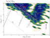 |
Fig. 3 Phase-space distribution of asteroids around the Sun ~100 Myr after escape from its parent cluster. The shaded region presents a kernel-density estimation of the simulation results, representing various families of objects. We adopted a non-parametric Gaussian kernel density estimator with a symmetric bandwidth of 0.02 (Scott 1992). At this moment, part of the Oort cloud is already in place (to the right), but the formation process is still ongoing. The colored diagonal curves (from top left to bottom right) indicate orbits that cross those of the giant planets (see also Fig. 1). The dashed burgundy colored curve to the right indicates where the orbital period, Porb, is equal to the eccentricity damping-diffusion timescale by the Galactic tidal field (tdiff, Eq. (5) of Duncan et al. 1987). The solid black curves indicate the Galaxy’s perturbing influence in terms of the velocity-kick imparted to an object. Relative velocity perturbations of δv = 10−3 (right), 10−5, and 10−8 (left) are indicated. The little area to the right of Neptune’s influence (between the red diagonal curve and the black curve indicating a perturbation δv = 10−8) corresponds to the Kuiper-belt kernel distribution. The parking zone is indicated in red. The Oort cloud is to the right of the rightmost solid black curve (labeled as δv = 10−3) and the burgundy colored dashed curve. The Hills cloud is to the left of this dividing line (indicated in black). In our simulations, the Hills cloud at low eccentricity (e ≲ 0.95) is mostly empty, but at higher eccentricity (near the bottom of the figure) its population is substantial, in particular along the conveyor belt. The captured and scattered asteroids are indicated in white contours. Locally, at the extreme, both populations have comparable phase-space density. At the age of 100 Myr, a considerable fraction of the native disk population has already reached the Oort cloud, or is on its way there through the conveyor belt. Some captured asteroids are currently migrating along the conveyor belt and a few have already reached the Oort cloud. However, the majority of the scattered and captured asteroids are in the parking zone between ~ 100 au and ~ 1000 au, where they will stay for the duration of the simulation. Jupiter and Saturn eject asteroids along the conveyor belt into escaping orbits (indicated in orange). Uranus and Neptune eject asteroids on a timescale considerably longer (≳ 100 Myr) than that for Jupiter and Saturn (≲10 Myr), allowing these asteroids to be circularized by the Galactic tidal field (also in orange). This is also visible in the lower kernel density along the Jupiter–Saturn conveyor belt in comparison with the Uranus–Neptune conveyor belt. Eventually, the latter asteroids become members of the Oort cloud. The red dotted curve indicates the Hill radius of the Sun in orbit around the Galactic center, here at about 0.65 pc. The thin dotted diagonal curves indicate pericenter distances of 1 au and 1 R⊙. Comets from the Oort cloud may enter the inner Solar System (to the far bottom right and below the 1 au curve). |
3.2 Evolution of the circumstellar disk of an isolated Solar System
The simulations presented in this section are designed to help us to understand the consequences of evolution of the newly born Solar System witha disk of planets and asteroids as part of the Galactic tidal field. The Solar System is initialized in the Galactic potential at − 8.4 kpc along the x-axis and 17 pc above the Galactic plane. The initial velocity of the Solar System was v⊙ = (11.352, 233.105, 7.41) km s−1, which follows an almost circular orbit around the Galactic center (see Fig. 4). From this position and velocity we calculate the position of the Sun in the Galaxy backwards for 1 Gyr, which is where our calculations start. The location of the Solar System 1 Gyr ago was (−4.451, 7.796, 53.99) kpc, with a velocity of (204.1, 101.3, 5.742) km s−1.
We initialized the Solar System with the four giant planets, Jupiter, Saturn, Uranus, and Neptune, as they appear in their orbit on 1 January 2020 (2020-01-01T00:00:00.000 UTC), according to the JPL Horizons database4. (We note here that the choice of the initial epoch should not considerably affect either the qualitative or the quantitativestatistical results. However, for the orbits of individual asteroids, the precise initial realization is important; see Sect. 4.4.2 for a brief discussion). The ecliptic was initialized with an angle of 60° to the Galacticplane. The initial conditions for these simulations are presented in Table 2. A wider range of initial realizations was tried, including changing the orbital phases, and separations of the planets and the parameters for the debris disk (see Sect. 4.1). Varying the orbital phases does not result in qualitative differences, but the results are relatively sensitive to changes in the initial orbital separations of the planets. After initializing the planets, we place a disk of test particles in the ecliptic plane around the Sun. The disk was generated using the routine ProtoPlanetaryDisk in the AMUSE framework with a Toomre-Q parameter of 25 (Toomre 1964). Most simulations are performed with disks of between 16 au and 35 au, but other ranges were explored with a minimum of3 au and an upper limit of 1000 au.
In the simulations, Jupiter starts to populate the resonance regions (such as the asteroids of the Hilda-family; in Fig. 1 the purple arrows to the bottom left illustrates how they migrate) and launches asteroids into the conveyor belt (light green and black curves) directly from the start of the simulation. This process happens very early after the formation of the Solar System which may then still be a cluster member. After 1 Myr, 43.4% of the asteroids born between 3 and 15 au are still in resonant orbits, and 39.4 % have escaped the Solar System (see also Pirani et al. 2018, 2019). Asteroids initially on wider orbits are not affected much within this short time-frame. Figure 5 illustrates this process by plotting the orbit of a test particle integrated with the Solar System and the tidal field of the Galaxy.
On a longer timescale, based on the simulations listed in Tables 4 and 1, the ice-giant planets transport asteroids along the conveyor belt into the Oort cloud, where they slowly circularize and isotropize. After ~ 100 Myr, the orbital distribution of asteroids is similar to that of the present epoch; the stable resonant regions near the giant planets are populated, and the non-resonant orbits as well as the conveyor belt are depleted. Only 1.4 % of the asteroids born between 15 and 50 au are still in the disk after 100 Myr and 59.2% have become unbound from the Solar System. The remainder of the asteroids born between 15 and 50 au have migrated to the Oort cloud at this point in time.
The giant planets only scatter the asteroids in inclination by a few degrees (see also Di Sisto & Rossignoli 2020). By the time the asteroids reach the inner Oort cloud, their inclinations are still not much larger than a few tens of degrees around the ecliptic plane. Even asteroids that are scattered along the conveyor belt to the Oort cloud preserve a relatively low inclination with respect to the ecliptic plane (see also Duncan et al. 1987; Correa-Otto & Calandra 2019). The inclination distribution only isotropizes once the Galactic tidal field starts to dominate the orbital evolution of the asteroids (see also Fouchard et al. 2018). Although the majority of the asteroids escape the Solar System while being kicked out by the planets, the number that remain bound is sufficient to explain the richness of the predicted population of objects in the Oort cloud.
Nevertheless, the schematic view presented above is rather idealized because we assume that the Solar System was born as a single star orbiting in the Galactic potential. In the following section, we relax this assumption and study the consequences of the Sun being born in a young stellar cluster. It turns out that being born in a clustered environment has profound consequences for the efficiency of the formation of the Oort cloud.
Model parameters of the Milky Way.
3.3 The evolution of the Solar System in its birth cluster
For the simulations presented in this section, the Solar System is initialized as a member of a star cluster (see also Torres et al. 2020a; Stock et al. 2020; Veras et al. 2020). Two series of simulations were performed: one in which the Sun has four giant planets in a compact configuration, and the other that shows a more extended configuration (see Table 3). Simulations are performed with 2000 asteroids in circular orbits of between 16 au and 35 au for the compact, and another series with asteroids in circular orbits of between 40 and 1000 au for the extended configuration (see also Torres et al. 2020a). An additional set of 32 simulations (not listed in Table 3) was performed in which the Solar System, with a disk of 1000 asteroids, experiences a single close encounter at a distance of 225 au or 400 au with a relative velocity of 1 km s−1. Here we varied the impact angle of the encountering star from 0° (in the ecliptic plane) to 30°, 60°, and 90° (perpendicular to the ecliptic).
In these models, we ignore the inner disk (within 40 au for the extended models and within 16 au for the compact models). This is motivated by the fragility of the inner Solar System. Any encounter that would perturb the inner region would probably leave the Solar System unrecognizable today. Therefore, there seems to be no particular reason to include the inner disk in the calculations. Each simulation was performed up to 100 Myr. This timescale is smaller than the cluster lifetime, but is sufficient to support the conclusions of this paper.
The cluster in those simulations is built using NBODY6++GPU (Wang et al. 2015), while we use REBOUND (Rein & Liu 2012) to integrate the planetesimals (using the IAS15 integration scheme from Rein & Spiegel 2015). The simulations are carried out using the LonelyPlanets approach designed in Cai et al. (2017, 2018, 2019).
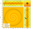 |
Fig. 4 Galactic distribution of asteroids 1 Gyr after the Sun escapes its birth cluster (still ~ 3.6 Gyr in the past). The colored background represents the adopted Galaxy potential: bottom left, top left, and bottom right views show the various Cartesian coordinates (the bar is not shown). The red and green dots show the bound and unbound asteroids. The starting position of the Sun is also indicated. The top-right corner panel shows a magnified view of 6 pc by 6 pc around the Sun. The outer circle shows the Hill radius at ~ 0.65 pc, and the inner circle represents the inner edge of the Oort cloud at about ~ 0.21 pc (at δv = 10−3). |
3.3.1 Simulating planetary systems in a dense star cluster: the LonelyPlanets approach
In the LonelyPlanets module in AMUSE, we first evolve a star cluster without planets or asteroids for 100 Myr using NBODY6++GPU (Wang et al. 2015). This calculation includes the N-body dynamics of the stars, stellar evolution, and the interaction with the Galactic tidal field (as described above). Clusters are born instantaneously without residual gas and with stars from a mass function on the zero-age main sequence distributed in a virialized Plummer sphere. We store masses, positions, and velocities on the five nearest neighbors for each star during the calculation at 1000-year time intervals. Interactions with a single nearest star provided satisfactory statistics for the strongest encounters (Glaser et al. 2020), but in our opinion lacked the weaker perturbations. We therefore include the nearest five stars.
In the second pass through the data, each stored encounter is treated as a scattering experiment lasting 1000 yr. After each scattering experiment with five perturbing single stars and one star with planets, we continue with the new set of five perturbing stars while carrying the planetary system over from one scattering experiment to the next, 1000 years later. This works as follows. The masses, positions, and velocities of the five perturbing stars are recovered from file, and the target star with planets and test particles as asteroids is integrated together with the perturbers (see Table 3). After 1000 years of integration, we recover the next set of five perturbers from file and integrate them as a new experiment together with the target star, planets, and asteroids. We note that these five nearest neighbors may be different stars from one snapshot to the next (1000 years later). The presence of planets in the scatter experiment leads to small perturbations of the encountering stars, which affects their orbits. Therefore, even if a subset of perturbing stars is identical from one snapshot to the next, the positions and velocities of these perturbers does not necessarily have to be identical at the end of a scatter experiment and the beginning of the next snapshot because the encounter database was built without planets. Our approach is therefore inconsistent.
The encounter between the five perturbing stars and the one star with planets and asteroids is calculated using REBOUND (Rein & Liu 2012). This process is repeated for each encounter for the duration of the star-cluster simulation (100 Myr). Figure 6 presents an illustration of this method with the six interacting stars identified.
In the following two sections, we discuss two populations: the captured and the scattered populations of asteroids. The amount of mass (or the number of asteroids) that is transferred is similar to the number of asteroids at the periphery of the disk, which is unbound or scattered into highly eccentric and inclined orbits (Jílková et al. 2015).
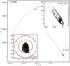 |
Fig. 5 First 2 Myr of the orbital evolution of an asteroid born in a circular orbit in 4:5 mean-motion resonance with Jupiter. Repeated interactions with the giant planets (colored circles: blue, orange, green, and red for Jupiter, Saturn, Uranus, and Neptune, respectively) launch the asteroid along the conveyor belt into the Oort cloud until it reaches the Hill sphere at a semi-major axis of ≳ 14 000 au with eccentricity ≳0.995. The inset tothe lower left gives the first 0.1 Myr of evolution, and the inset to the top right gives the first 0.3 Myr. Each frame is on a different scale. |
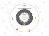 |
Fig. 6 Illustration of the extended Solar System model (not to scale). The gray shaded region represents the debris disk with an outer radius of 1000 au. The dotted red circle indicates the boundary of the neighboring sphere, beyond which we ignore the influence of perturbations by passing stars. Gray symbols represent the stars in the cluster that are ignored. The colored star symbols (P1, P2, P3, P4, and P5) represent the five nearest stars that perturb the Solar System at a given time. The arrows indicate the direction of motion of the perturbers (figure from Torres et al. 2020a). |
3.3.2 The influence of the cluster on the circumstellar disk
When a staris a young cluster member, mutual encounters affect the circumstellar disks (Vincke et al. 2015; Vincke & Pfalzner 2016). However, most simulation studies address the effects of one star on the disk of another star resulting in the deformation of the disks (Breslau et al. 2014; Rawiraswattana et al. 2016; Xiang-Gruess 2016; Breslau et al. 2017). A star in a cluster is exposed to multiple encounters, each having a subsequent effect on the disk’s morphology and mass. Only a few studies take these multiple interactions into account (Jiménez-Torres 2020; Torres et al. 2020a).
Moreover, mutual interactions also lead to the transport of material from one star to another (see also Korycansky & Papaloizou 1995). We address both processes separately. Here we describe the scattering of the native disk due to stellar encounters. In Sect. 3.3.3, we discuss asteroids that are abducted from the disk of another star.
In the calculations with LonelyPlanets, we follow the dynamical evolution of the debris disk and planets around each star individually (see previous paragraph). The disks are only resolved in the second pass through the data. As a result, disks do not interact mutually, but they are affected by multiple encounters with other stars.
Each star experiences multiple interactions with other stars. We focus on one particular star in this simulation: the 1 M⊙ star # 157 from Torres et al. (2020a, their Fig. 2). We picked this star because the orbital topology of its scattered population resembles the Kuiper belt of the Solar System. The initial inner edge of the disk in this calculation is 40 au. This seems rather large, but a strong perturbation of the more inner region would have had considerable repercussions for the entire planetary system, contrary to what is observed in the Solar System.
In Fig. 2, we present the orbital distribution of the scattered disk population (green dots). The small black lines from each dot point in the direction of the evolution of its orbit over the next 300 Myr. The population near the inner part of the disk (a ≲ 50 au) is affected by the outer planets, causing an increase in their eccentricity. The population between 50 and 500 au is hardly affected by either the planets or the other stars, and is hardly affected over the lifetime of the Solar System, until the Sun evolves beyond the main sequence and sheds its outer layers (this process was studied extensively by Veras et al. 2011, 2014; Veras & Tout 2012; Zink et al. 2020).
Once the star and surviving disk leave the parent cluster, ~ 4.2 % of its native outer-disk asteroids have been scattered through interactions with other stars directly into the conveyor belt region. The majority of these asteroids move on a timescale of ~ 100 Myr along the conveyor belt until they reach the Oort cloud (once they cross the curve tdiff = Porb, or the curve of δv = 10−3). This process is illustrated in Fig. 2 with the long lines that start at the asteroids and point to their orbital parameters 300 Myr later in time (in the direction of the Oort cloud). We note that in Fig. 2 the curve for δv = 10−5 is given, which roughly corresponds to the inner edge of the Hills cloud. The difference between the δv = 10−5 and δv = 10−3 is also illustrated in Figs. 1 and 5.
After ~100 Myr, some asteroids of ≳2.5 Neptune-Hill radii from the orbit of Neptune are still in the process of ascending the conveyor belt (see the thin dotted curve to the right of the red curve in Fig. 2). This small population of asteroids within the conveyor belt does not migrate to the Oort cloud. Di Sisto & Rossignoli (2020) found a similar population of lingering asteroids, and the migration process in their calculations takes ~ 68 Myr, which is comparable to the ~100 Myr in the calculations presented here. Also, Fernández et al. (2004) studied the migration rate of scattered trans-Neptunian objects to the Oort cloud and argue that eventually, after 5 Gyr, half the scattered disk settles in the Oort cloud.
3.3.3 The captured asteroids
Apart from scattering of the circumstellar disk, stellar encounters also lead to the capture of asteroids. The majority are deposited in the parking zone, possibly in highly inclined orbits (Jílková et al. 2016). Those that enter the conveyor belt migrate towards the Oort cloud or are ejected. The fraction of captured asteroids that enter the conveyor belt depends on the details of the encounter, and the disk parameters of the encountered star. Although the numbers vary strongly depending on the parameters of the encounter, the typical fraction of captured asteroids is comparable to the fraction of asteroids lost, at least in an equal-mass encounter (see also Breslau et al. 2017). Encounters in which the encountering star meets the prograde orbiting debris disk are most effective in producing unbound asteroids (Pfalzner et al. 2021). The population of captured asteroids may therefore have a high proportion of retrograde orbits compared to those ejected from the inner Solar System.
We included a population of captured asteroids in our analysis. However, the calculations using the LonelyPlanets approach are not suitable for acquiring a census of their orbital distributions (Cai et al. 2018) because once an asteroid becomes unbound from its parent star it is lost from the simulation. Instead of taking the results of system # 157 from Torres et al. (2020a), as we did for the scattered disk, we adopt the results of Jílková et al. (2015) for the captured asteroids. These latter authors performed N-body calculations to study the mutual stellar encounter that could explain the orbit of the dwarf planet Sedna. They argue that Sedna was captured from the circumstellar disk of another star. This must have happened while both stars were members of the same parent cluster. The captured population from Jílková et al. (2015) reproduces Sedna’s orbit as a captured object.
At present, Sedna is orbiting in the parking zone well outside the conveyor belt and is not expected to reach the Oort cloud. From a Galactic point of view, Sedna is relatively close to the Solar System. Asteroids within ≲ 1000 au of the parent star are hardly affected by the tidal field of the Galaxy. The parking zone is therefore composed of a roughly equal number of scattered and captured asteroids. The orbits of asteroids in the parking zone are no expected to be affected by either the planets or by the Galactic field. Frozen in time, this population may bear information about the mechanism that brought it there.
We introduced the captured population into the Solar System and integrated it as test particles together with the giant planets and the background potential of the Galaxy over a timescale of 300 Myr5. The simulations are summarized in Table 2. The resulting orbital parameters are presented in Fig. 2.
During integration, the captured asteroids that were introduced in the conveyor belt region have been driven by the giant planets into the Oort cloud region. The timescale on which they reach the Oort cloud depends on their relative inclination to the ecliptic, and on the pericenter distance. Highly inclined asteroids, for example, may have their closest approach to the Sun far from the perturbing influence of the giant planets. Asteroids orbiting in the ecliptic plane are more strongly affected by the giant planets, and are scattered into the conveyor belt on a shorter timescale.
3.3.4 When did the Sun escape the parent cluster?
Here, we assume that stars form instantaneously in random positions from a point-symmetric Plummer (1911) potential in virial equilibrium. Planets also form instantaneously in almost circular orbits in a randomly oriented ecliptic plane.
These are strong (and, in our view, rather preposterous) assumptions, and some of our results are affected by these choices. However, relaxing any of these assumptions will open up parameter space and lead to a dramatic increase in the number of calculations required to acquire reliable uncertainties on the simulation results. One improvement would be to take the hydrodynamical collapse of the molecular cloud into account, including the processes of star formation, stellar feedback, disk evolution, and planet formation. However, these calculations are somewhat elaborate (Calura et al. 2020; Fukushima & Yajima 2021).
Even though the processes discussed in this paper are fundamental, the timescales and efficiencies of the various processes are affected by the initial conditions of the simulations (Adams et al. 2006). The timescale over which, and the order in which, the giant planets form are important for the presented model and the efficiency at which asteroids are injected into the Oort cloud. The conclusion that asteroids were ejected early on by the giant planets while the Sun was a cluster member remains largely unaffected. The Oort cloud will be prevented from forming so long as the Sun is a member of a star cluster (Higuchi & Kokubo 2015). Only after the Sun has left the birth cluster is it possible to keep asteroids bound in orbits as wide as the current Oort cloud up to the Hill radius in the Galactic potential.
It is not trivial to constrain the moment at which the Sun escaped its birth cluster. In the first ≲ 10 Myr, the cluster is expected to have a relatively high density ≳103 M⊙ pc−3 (Lüghausen et al. 2012; Martínez-Barbosa et al. 2016; Pfalzner & Vincke 2020; Pfalzner et al. 2020). After that, the cluster expansion is driven by stellar winds, radiation feedback, and supernovae until it eventually dissolves in the Galaxy’s tidal field. This latter phase in which the cluster dynamics is dominated by two-body relaxation and tidal stripping lasts for approximately 100 Myr (Adams et al. 2006; Stock et al. 2020). While the cluster expands with time, the local density gradually decreases, and the encounter rate drops (Baumgardt & Kroupa 2007; Cai et al. 2017). These time scales are all short compared to the formation timescale for Jupiter of ≲ 4 Myr (Kruijer et al. 2017; Movshovitz et al. 2010; D’Angelo et al. 2021).
The Solar System may have survived this first dense phase rather unharmed, leaving the cluster at a later stage, possibly around the cluster’s half-life timescale. According to our calculations (but also see Kaib & Quinn 2008), it seems more difficult to grow a rich Oort cloud if the Sun stays in the parent cluster for ≳ 100 Myr, because thiscorresponds to the timescale on which the ice-giant planets eject their local asteroids into the conveyor belt. We therefore argue that the Solar System might have been ejected from the parent cluster within ~ 20 or 50 Myr after birth.
The effect of a nearby encounter on the cold Kuiper belt may not have had a long-lasting impact, as this population might have regrown over time (Astakhov et al. 2005; Punzo et al. 2014; Moore et al. 2020). Other signatures of the difference between a few strong encounters and extended exposure to relatively weak perturbations are hard to quantify. We did not explore the long-term survival of the Solar System in its birth cluster and its possible consequences for the outer edge of the planetary disk. It would be interesting to study this aspect, but these calculations are elaborate, and the parameter space is extended.
3.4 Eccentricity damping of the asteroids in the Oort cloud
While the gas-giant and ice-giant planets launch asteroids further into the Oort cloud, the Galactic tidal field gradually becomes a stronger perturber. Eventually, when asteroids cross the purple-dashed curve in Fig. 2 (far to the right, but more visible in Figs. 1 and 3) their orbits become strongly affected by the Galactic tidal field through von Zeipel-Lidov-Kozai resonance (von Zeipel 1910; Lidov 1962; Kozai 1962); (see Ito & Ohtsuka 2019, for a historical overview on the terminology). This leads to damping of the eccentricity (as is also demonstrated in Vokrouhlický et al. 2019). In our simulations, this proceeds through a random walk in semi-major axis and eccentricity but directed towards lower eccentricities. In Fig. 7 we illustrate this process with three asteroids from one of our simulations. These particles start in the narrow neck between 1000 au and 3000 au at an eccentricity ≳ 0.998 while they are kicked by one of the giant planets along the conveyor belt into the Oort cloud region. The tidal field of the Galaxy subsequently reduces the orbital eccentricity of these asteroids. This eccentricity-damping process proceeds as a random walk in eccentricity and orbital separation. The influence of the Galactic tidal field near the apocenter of the asteroid may cause the orbital eccentricity to increase as well as decrease, whereas the semi-major axis is less strongly affected. The global trend is a reduction in eccentricity. Asteroids further in the Oort cloud are more strongly affected by the Galactic tidal field, and therefore have a shorter circularization timescale. Not all asteroids circularize to the low eccentricities of the three examples presented in Fig. 7. Eventually, after a few hundred million years, we find empirically that the cumulative probability density function for the eccentricity approaches  . Figure 8 presents the evolution of the eccentricity distribution of the Oort cloud (four lower curves). Table 4 presents the conditions for the simulations that support this section.
Asteroids in the disk start with almost circular orbits (uppermost blue curve in Fig. 8). In time, this distribution becomes more skewed to higher eccentricity, mainly due to the injection of objects into the conveyor belt (orange curve). The scattered and captured asteroid populations have, upon capture, a steeper eccentricity distribution (purple curve), which approaches the thermal distribution (dotted curve).
A fraction of the disk particles together with some of the scattered disk and captured asteroids migrate further along the conveyor belt until their eccentricity distribution resembles the lowest (red) curve in Fig. 8. This latter distribution continues to evolve over time until it resembles the purple curve (indicated with the Oort cloud at 1 Gyr). Further evolution of the Oort cloud is slow, on a timescale of ≳ 1 Gyr, and is dominated by evaporation. By counting the number of objects that re-enter the inner Solar System, we derive a rate of ~ 2–6 × 10⁻¹² comets per asteroid in the Oort cloud per year that find their way back into the inner Solar System within 10 au (see Sect. 4.2.3). This leads to one or two comet arrivals in the inner Solar System per year, which is consistent with earlier estimates (Byl 1986; Heisler & Tremaine 1986; Gardner et al. 2011; Fouchard et al. 2020).
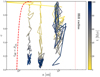 |
Fig. 7 Orbital evolution of three asteroids for 100 Myr in semi-major axis and eccentricity. Each starts from the conveyor belt (to the top left) until it circularizes. These asteroids are launched into the conveyor belt by a giant planet. This process is illustrated in Fig. 5. Once the Galactic tidal field starts to dominate the orbital evolution of the asteroids (to the right of the red dashed curve), it detaches them from the influence of the inner planets. The Galactic tidal field subsequently drives the eccentricity evolution of the asteroid until it circularizes. The timescale of the circularization process is illustrated with the color bar. Asteroids further in the Oort cloud are more strongly affected by the Galactic tidal field, and therefore have a shorter circularization timescale. Not all asteroids circularize to the low eccentricities of the three examples presented here. The eventual eccentricity distribution of the Oort cloud objects is presented inFig. 8. The vertical dotted curve to the right indicates the Hill radius of the Solar System in the Galactic potential. |
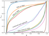 |
Fig. 8 Cumulative distribution of the eccentricity at various stages of the evolution of the eventual Oort-cloud population of asteroids. The dotted and dashed curves are presented to guide the eye. The dotted curve gives the probability density function for the thermal distribution in eccentricity (f(e) ∝e2). The dashed curve gives an eccentricity probability density function |

3.5 Summary of the chain of simulations
Now that we have briefly discussed each of the simulations, we can construct a more holistic view of the formation and early evolution of the Oort cloud. Here, we summarize this model and in the following section we discuss the consequences.
Asteroids in the conveyor belt cross the orbit of the giant planets. Each time this happens, they receive a small kick causing their orbits to drift with constant pericenter distance to higher eccentricity and larger semi-major axis (illustrated in Fig. 5, but see also Duncan et al. 1987). Jupiter ejects its nearby asteroids along this conveyor belt (indicated in Fig. 3) on a timescale of a few million years.
Once the eccentricity of an asteroid is ≳0.998 and its semi-major axis is ≳20 000 au, the Galactic tidal field starts to dominate the orbital evolution of the asteroid at apocenter (Higuchi et al. 2007, see Fig. 3). As soon as the pericenter distance exceeds the semi-major axis of the giant planet, the eccentricity of the asteroids’ orbit continues to be reduced. By this time, the orbital period is ≳ 3 Myr, and the Galaxy starts damping the asteroid’s eccentricity and randomizing the inclination (Higuchi et al. 2007) on a timescale of ~ 100 Myr (Duncan et al. 1987; Di Sisto & Rossignoli 2020).
Eventually, this process leads to the Oort cloud. The distance travelled by an asteroid into the Oort cloud depends on the last interaction with the planets before its orbit detaches (see Fig. 7). Once near apocenter, the Galactic tidal field reduces the eccentricity of the orbit, causing the pericenter distance to increase.
Our calculations did not last a sufficient length of time to circularize the entire population, but the reduction in eccentricity converged in ~1 Gyr to  . We therefore argue that the Oort cloud still hosts a considerable fraction of asteroids in relatively high-eccentricity orbits. This distribution in eccentricity is consistent with the one found in Higuchi & Kokubo (2015) at an age of 500 Myr to 1 Gyr. These latter authors further argue that the eccentricity distribution in the Oort cloud thermalizes in ~ 5 Gyr. We do not observe such a thermalization of the eccentricity distribution. The structure of the Oort cloud can then also inform us about what happened in the early Solar System (see also Fouchard et al. 2018).
The orbital distribution of the giant planets is not very important in this evolutionary sequence, except that more massive planets, upon their last interaction, can inject asteroids in wider orbits with a higher eccentricity.
The large mass and short orbital period of Jupiter clears the local asteroid field in as little as a few million years (Duncan et al. 1987; Fouchard et al. 2014b). Therefore, the Oort cloud cannot have formed from asteroids ejected by Jupiter or Saturn, because their ejection timescale is shorter (≲ 10 Myr) than the expected cluster lifetime of ≳100 Myr (Portegies Zwart et al. 2010). In Sect. 3.3.4 we conclude that the Sun escaped the parent cluster even before that time, that is, in 20–50 Myr. In the first million years after their formation, the giant planets launch ≳ 80.3% of the asteroids between 3 and 15 au onto the conveyor belt, and 57.0 % of these escape the Solar System within the next million years. Within ~ 10 Myr, all the asteroids born near Jupiter and Saturn are either deposited in resonances or escape the Solar System. Jupiter and Saturn therefore cannot have contributed much to the formation of the Oort cloud (this was also concluded by Torres et al. 2020a,b). However, the details depend on the relative timing of the various events and on the mass distribution within the disc. Constraining those more precisely would require more extended and sophisticated self-consistent simulations.
In our simulations, we ignore the star, planet, and asteroid-formation processes: all are born instantaneously. We have not explored parameter-space exhaustively, but argue that the details regarding the precise moment and the orbits in which the giant planets form are relevant only to second order because they affect the timescale for the formation of the Oort cloud but not the fundamental process.
The time scale over which asteroids are ejected by the planets is sufficiently long that an uncertainty of few million years in the planet-formation process (Kruijer et al. 2017) does not affect the efficiency of the ejection process. So long as the Solar System is a member of a star cluster, a sequence of distinct processes drive the formation of the Oort cloud.
4 Results and discussion
4.1 The birth environment of the Solar System
The birth environment of the Solar System plays a major role in the formation of the Oort cloud: It prevents the gas-giant planets from forming the Oort cloud, but at the same time stimulates its formation by scattering the outer regions of the circumstellar disk and by introducing new asteroids by capturing them from other stars, or from the interstellar free-floating population (see also Zheng et al. 1990).
The Oort cloud has, according to this view, only a minor contribution from the scattered asteroids originating from the gas-giant planets, Jupiter and Saturn. Apart from those asteroids parked in resonant orbits, these planets cause asteroids to escape the Solar System and become interstellar free-floating objects (see also Torres 2020; Torres et al. 2020a).
In contrast to Jupiter and Saturn, the ice giants, Uranus and Neptune, are more favorable in producing the Oort cloud (see also Leto et al. 2008; Paulech et al. 2010). They carry out the same process of ejecting asteroids, but do this, because of their lower mass and wider orbits, on a longer timescale and with smaller impulsive changes in eccentricity and semi-major axis of the asteroids (see also Duncan et al. 1987; Fernández et al. 2004; Correa-Otto & Calandra 2019).
The longer timescale on which the ice-giants planets eject asteroids is important for the formation of the Oort cloud because so long as the Solar System is a member of the parent cluster, asteroids in wide orbits are easily lost from the Solar System (Nordlander et al. 2017). This process of asteroid stripping due to encounters with nearby stars is particularly effective if the asteroid’s orbit is wide and highly eccentric. After a few tens of millions of years to ~ 500 Myr, once the Solar System has escaped the parent cluster, such asteroids can remain bound.
The wide and highly eccentric orbits of new arrivals in the Oort cloud can subsequently be perturbed at apocenter by the Galactic tidal field, leading to a reduction in their eccentricity through von Zeipel-Lidov-Kozai resonance. As a consequence, the pericenter distance of these asteroids increases, which brings them outside the influence of the planets and detaches them from the conveyor belt. While the orbital eccentricity of the asteroids continues to decay due to the Galactic tidal field, they slowly, over a timescale of ~ 100 Myr, form a distribution of very wide but relatively low-eccentricity orbits The distribution has to shape of the tidal lobe of the Solar System in the Galactic potential. The size of the Oort cloud is confined on the inner side to the distance where the Galaxy starts to influence the orbits of the asteroids (at a relative velocity change of δv ≳ 10−3), and at the side furthest from the Sun in the Galactic potential by the surface of the Hill sphere (illustrated in Figs. 1 and 6).
According to Leto et al. (2008), the number density in the Oort cloud is proportional to n ∝ r−3.53, whereas we find a considerably more complex structure. In the Hills cloud and Oort cloud, we find n ∝ r−2.25, with an overall flatter slope of − 2.57 for the entire range from 100 au to the Hills radius (see Fig. 9). The slope of the density profile of ~ − 2.25 between 2 × 10⁴ au and 105 au is somewhat shallower than the slope of ~−4.0 by Higuchi & Kokubo (2015), that of ~−3.35 found by Vokrouhlický et al. (2019), or that of ~−3.0 by Leto et al. (2008). Higuchi & Kokubo (2015) argue that this slope is independent of the mechanism that brings asteroids to the Oort cloud, but that does not explain the differences in the density profile between these different studies. Part of this structure may be the result of orbital evolution of the Solar System and its possible migration inthe Galaxy (Rickman et al. 2008; Kaib et al. 2011a,b), but another part may be the result of planetary migration (Fouchard et al. 2018).
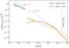 |
Fig. 9 Density profile of the initial circumstellar debris disk (blue, to the top left) and the eventual Oort cloud, ~ 1 Gyr after the Solar System left the parent cluster (orange). The red dotted line to the right indicates the formal Hill radius of the Sun in its orbit around the Galactic center. The thin-solidblack-dotted curve shows the initial density profile of the circumstellar disk of ∝ r−2.5 (from simulations of Table 4). The thin dotted curve shows the density profile ∝ r−3.5 which, according to Leto et al. (2008), resembles the slope of the density profile of the Oort cloud. In our calculations, the distribution is somewhat shallower, but not as shallow as found by Higuchi & Kokubo (2015) who argue in favor of ∝ r−2.0, which is presented here with green dashes. The small tail of asteroids beyond the Solar System Hill radius in the Galactic tidal field has contributions of a minority of asteroids that remain bound to the Sun, and those that slowly move away. |
4.2 Results
4.2.1 The Sun in the Galaxy
A small fraction (~0.59 ± 0.1%) of the Oort cloud population on the far side of the Hill surface remains bound to the Sun (see Fig. 9). At an age of 1 Gyr in our simulations, this population has an eccentricity of ⟨e⟩ = 0.80 ± 0.23 with an inclination of ⟨i⟩ = 96° ± 42. These orbital parameters are similar to those of the Oort cloud asteroids within the Sun’s Hill surface, and they are consistent with the population presented in Fig. 7 of Vokrouhlický et al. (2019). The objects at the far side of the Hill surface (beyond ~ 200 000 au), are not expected to stay there long as they are ionized from the Solar System by close stellar passages in the Galactic field (Correa-Otto & Calandra 2019).
Asteroids ejected from the Solar System become free-floating interstellar objects. This latter population forms a trail of asteroidal objects in the Galaxy along the orbit of the parent star (Correa-Otto & Calandra 2019; Torres et al. 2020a; Tutukov et al. 2020; Portegies Zwart 2021). As the asteroids have a low velocity relative to the orbital speed of the Solar System, they continue to follow the same orbit as the Sun (see Fig. 4). Long after they have become unbound, these asteroids still orbit in a cloud around the Solar System distributed along extended trailing and leading arms (see also Tutukov et al. 2021). Eventually, these trails may be perturbed and scattered by passing molecular clouds or other stars, scattering their orbits and widening their phase-space distribution (see Martínez-Barbosa et al. 2016; Pfalzner et al. 2020; Torres et al. 2020a).
4.2.2 Consequences of planets in resonant orbits
We performed several additional simulations to study the consequences of planet migration in the early Solar System. In Tables 6 and 1 we present an overview of these calculations. In addition to the currently observed distribution of orbits for the giant planets, we also simulated a more compact configuration and a resonant configuration. The main problem in exploring these initial conditions lies in the enormity of the initial parameter space to be covered; our parameter-space coverage is far from complete. We therefore selected a few cases which have been of some interest in the past (see e.g., Wyatt 2003; Gomes et al. 2005; Malhotra 1998; Crida et al. 2007; Brunini 2019).
In one of these cases, we initiate a Nice-like planetary orbital distribution and a disk between 3 au and 50 au. In that configuration, Jupiter was placed on a circular orbit at 5 au in the ecliptic plane, and the subsequent planets in 2:1 mean-motion resonances with the one closer to the star. We also tried other configurations (see Table 4). The main conclusion, namely that the gas-giant planets (Jupiter and Saturn) eject asteroids on a timescale shorter (≲ 10 Myr) than the expected survival timescale in the parent cluster (≳100 Myr), also holds for these initial conditions.
Changes in the orbital distribution of the giant planets affect the location and efficiency of the conveyor belt, and the timescale on which asteroids migrate along the conveyor belt. In our initial resonant configuration, the entire disk, up to the orbit of the outermost planet, at around 15 au, is cleared within 1 Myr. The area slightly outside the outermost planet, up to a distance of 20 au from the star, is cleared within a few million years. By the time the Solar System leaves the parent cluster, there are too few asteroids left to populate the Oort cloud.
Pirani et al. (2019) also simulated the early Solar System including the migration of the giant planets. Although these latter authors focused on the inner Solar System and the populations of resonant and Trojan orbits, their conclusions are consistent with the results of the calculations presented here. Planets in an initial resonant configuration are excluded based on the consequence that the majority of asteroids would be lost well before the Sun escapes the parent cluster. This also accounts for Uranus and Neptune; if they are born in (near) resonance, the chaotic reorganization of the Solar System would eject most of the asteroids in the disk on a timescale shorter than the expected lifetime of the Sun in the parent star cluster. Asteroids outside the outermost planet would be affected by resonant reorganization of the planetary orbits, but these asteroids are not likely to migrate into the conveyor belt, and therefore are not expected to arrive in the Oort cloud. Fully resonant initial conditions can therefore be omitted based on the existence of the Oort cloud, except for the part of the Oort cloud formed from material that was accreted from other stars or from free-floating debris.
Even if a resonant configuration in the ice-giant planets could lead to a dramatic change in the distribution of orbital parameters after ~ 100 Myr, as is advertised in the original Nice model (Gomes et al. 2005; Morbidelli et al. 2005; Tsiganis et al. 2005), the number of asteroids has already reduced below the number needed to explain the Oort cloud. We therefore argue that a system in which the planets are born close to resonance, or in which planets migrate in the first few million years since formation (such as advertised in the grand-tack model; Walsh et al. 2011), is unlikely to lead to the formation of an Oort cloud. Planetary migration after the Oort cloud formed has no further consequence for the Oort cloud, and we cannot exclude such evolution (Valtonen & Innanen 1982). Nevertheless, again, resonant initial conditions for the planets cannot be excluded if the majority of the Oort cloud material was accreted.
Simulations of a hypothetical young Solar System with planets in various orbital configurations.
4.2.3 Retrograde and re-entry orbits
We measure the fraction of asteroids in retrograde orbits. At the age of 300 Myr, well after the Sun escaped the cluster, 8.1 ± 0.3% of the scattered asteroids (a ≳ 100 au) have retrograde orbits, and for the compact resonant initial conditions this fraction is 7.1 ± 0.5%. In comparison, 71.9 ± 0.3% of the captured asteroids (a ≳ 100 au) have retrograde orbits. However, this latter fraction depends notable on the encounter parameters and the number may vary considerably for other simulations. Once well along the conveyor belt (at a(1 − e) ≳ 50 au and eccentricity ≳0.998), about 57 ± 1 % of the asteroids have retrograde orbits. This large fraction of retrograde orbits in the conveyor belt indicates the moment that the Oort cloud becomes spherical and isotropic. By this time, the orbits have also reached their terminal distribution in eccentricity (which is not thermal; see Fig. 8).
Because of interaction with the tidal field, a small fraction of asteroids return to the inner Solar System after having spent some time in the Oort cloud. We find 0.6 ± 0.1% of the asteroids that were launched from the conveyor belt into the Oort cloud return into the inner 10 au of the Solar System on a timescale of 1 Gyr. This results in a re-entry rate of 2 to 6 × 10⁻¹² yr−1. The re-entry rate for approaching the Sun to within 1 au is an order of magnitude smaller. The observed rate of observable comets in the Solar System, measured between 110 BC and 1970, was remarkably constant at a rate of 0.86 ± 0.067 per year (Licht 1999). A larger rate of 6.4 × 10⁻¹² per year was derived by Dones et al. (2004a), but they accounted for perturbations in the Oort cloud due to passing stars, which we neglected in our calculations. With our derived re-entry rate of comets within 1 au of the Sun of ~ 6 × 10⁻¹³ yr−1, and a total number of ~1012 cometary bodies in the Oort cloud, we derive a rate of about two new comets every 3 yr. Even when taking the tidal field and passing stars into account, our derived rate is somewhat on the low side compared to observations. The presence of a planet in the Oort cloud would pose an interesting possibility in increasing the cometary influx rate (Fouchard et al. 2014a; Ito & Higuchi 2020; Batygin & Brown 2021).
4.3 Interstellar comets
According to the simulations presented here, the Solar System is a copious polluter of interstellar space (Torres et al. 2019; Pfalzner et al. 2021); interstellar comets produced in this way could have characteristics similar to ’Oumuamua or Borisov (Higuchi & Kokubo 2020). This pollution predominantly happens in four rather distinct phases in the evolution of the Solar System: (A) while being a cluster member, when encounters between stars cause debris from the circumstellar disk to escape; (B) while the giant planets (Jupiter and Saturn) eject most of the asteroids within their gravitational influence; (C) after the Sun ascapes the cluster, and the ice giant planets (Uranus and Neptune) start kicking out asteroids; and (D) eventually due to the Sun’s copious mass loss while ascending the asymptotic giant branch and evolving into a white dwarf, causing asteroids to become unbound (Veras et al. 2011, 2014, 2020; Veras & Tout 2012).
According to Cai et al. (2019) 20–80% (with an average of 50%) of the circumstellar material survives the first 100 Myr of its evolution in the parent cluster. The majority of this mass is lost through encounters with other stars. The amount of material lost from the Solar System in the simulation presented here falls within this range, meaning that the circumstellar disk has lost about half of its mass due to interactions with other stars in the parent cluster, or about 100M⊕ to 3000M⊕. Each of the other processes results in a mass loss of roughly 20%. A small fraction of the ejected asteroids acquire bound orbits in the Oort cloud.
With an estimated mass of the Oort cloud of ~ 1013 kg comet−1, and a Hill radius of ~0.65 pc, we arrive at a density of ~ 1014 kg pc−3. If the Solar System had ejected ~90 % of its asteroids into interstellar space rather than forming an Oort cloud, interstellar space would have an average density of a few times ~ 1014 kg pc−3. This estimate is consistent with earlier estimates for the interstellar density of interstellar objects (Portegies Zwart et al. 2018; Do et al. 2018; ’Oumuamua ISSI Team 2019).
Regretfully, tracking a single interstellar interloper back to its origin is hindered by the uncertainties in the orbital parameters and the positions of stars in the past. Such tracking is limited to at most a few tens of millions of years (Zhang 2018). However, if multiple objects were found to have the same origin, tracking the orbit back in time could lead to a more precise determination of the original launching point (Portegies Zwart 2021). However, according to our calculations, most objects will have been ejected at an early stage while planets are still forming and migrating (see also Pirani et al. 2019). Possibly the star is even still a cluster member, in which case internal scattering with other stars will make it hard to trace the interstellar object back to a single star.
4.4 Discussion
4.4.1 Interpretations and caveats in the numerical approach
Numerical simulations are always affected by the choice of initial conditions and by numerical errors; either from the discretization of the underlying differential equations or by the exponential growth of round-off in the least significant digit. There is also the possibility of glitches or “bugs” in the simulations.
These uncertainties and errors become a particular potential cause of concern in chaotic systems. The outer parts of the Solar System, for example, have an estimated Lyapunov timescale ranging from ≲ 20 Myr (Applegate et al. 1986; Sussman & Wisdom 1988, 1992; Laskar 1990; Murray & Holman 1999; Farrés et al. 2013) to as much as 50 Myr (Laskar et al. 2011) or even exceeding the age of the Solar System (Grazier et al. 1999; Varadi et al. 2003).
Choices made in the initial conditions have considerable consequences for the numerical results and their interpretation. At the same time, numerical errors will also have repercussions for the conclusions in Sect. 5. Similar caveats in numerical work were acknowledged by Charles Babbage (1791–1871), the inventor of the difference and the analytical engines. Aware of these and other limitations, we describe the caveats in our approach in this section and discuss how to mitigate them.
4.4.2 Integration, symplecticity, and numerical errors
Newton’s equations of motion are intrinsically chaotic. Planetary systems are therefore also chaotic, as in the Solar System (Lecar et al. 2001; Valtonen et al. 2004). Chaos in the outer parts of the Solar System manifests itself as phase-bound or stable chaos (Milani & Nobili 1992; Saillenfest et al. 2019) and although it affects the stability of the Solar System (Todorović et al. 2020), it will not lead to a global unstable configuration (Tanikawa & Ito 2007). Chaos in the Solar System is driven by resonance overlap (Murray & Holman 1999, 2001). Even the Oort cloud is chaotic (Saillenfest et al. 2019).
Such chaos hinders the integration of the equations of motion for the Solar System; it renders these simulations notoriously unreliable for individual orbits. Possibly statistically they are trustworthy, meaning that the integrated bodies preserve the same phase space, but this has never been tested (for a discussion see Portegies Zwart & Boekholt 2018).
In this paper and many others, we rely on the statistical ensemble, averaging by numerical integration. It is widely suggested that, in these simulations, the conservation of energy is sufficient to preserve the final orbital parameter space. Symplectic integration methods are developed with precisely this objective, to preserve energy over secular timescales. Therefore, these methods arepopular for integrating planetary systems (Ito & Tanikawa 2002), but not for integrating star clusters or galaxies.
Although details in our calculations will depend on precise initial realization of the giant planets, the general results remain unaffected. We tested the effect of rather drastic variations of the initial conditions and the effect of subtle changes (such as the epoch of theSolar System), but we did not explore these systematically. The various simulation codes to perform this study are made public via the AMUSE framework, and we encourage others to continue exploring the parameter space.
5 Summary and conclusions
In our simulations, shortly after their birth, Jupiter and Saturn start to eject local asteroids from the circumstellar disk along the “conveyor belt”. Asteroids in the conveyor belt cross the orbit of the giant planets near their pericenter. Each time this happens, they receive a small kick causing their orbits to drift to higher eccentricity and larger semi-major axis while preserving pericenter distance. This process has been studied for asteroids whose pericenter is near Jupiter (Duncan et al. 1987; Fernández 1997). We confirm that Jupiter, with its relatively high mass and short orbital period, clears the local asteroid field in a few million years (Fernández 1997; Pirani et al. 2019). In Fig. 5, we illustrate this process by presenting one calculation where a single asteroid is ejected along the conveyor belt to reach the Oort-cloud region in a few million years. However, for the ice giants with their smaller mass and wider orbits, the process takes up to ~ 100 Myr (Fernandez 1981; Fouchard et al. 2013; Di Sisto & Rossignoli 2020), and if the asteroid has an inclined orbit, the process may last a gigayear.
While a member of a star cluster, an asteroid in a wide ≳ 103 au orbit is easily lost from the Solar System. A small perturbation in relative velocity of  is sufficient to unbind an asteroid. It turns out that asteroids on an eccentric orbit ≥0.98 and with a semi-major axis of ≳2400 au are vulnerable to being stripped from the Solar System. The period of such a wide orbit (≳ 0.1 Myr) is comparable to the mean encounter time between the Sun and another star in the parent cluster (assuming that the encountering star induces a similar perturbation in relative velocity). In the first million years after their formation, the giant planets launch ~ 80 % of the asteroids between 3 and 15 au onto the conveyor belt (see Sect. 3.5). Once there, the eccentricity and orbital separation of the asteroids rapidly increases.
The majority of the asteroids (~57 %) are moving along trajectories that become so wide that they are stripped within a few orbits, and within ~ 10 Myr most of the asteroids born near Jupiter and Saturn are either parked in resonant orbits (such as the Hilda family of asteroids) or their orbits have become so wide that they are easily stripped by passing stars in the parent cluster, and escape in about 20 to 50 Myr. The Oort cloud therefore cannot have formed in the first 10 Myr by Jupiter and Saturn ejecting asteroids because their ejection timescale is smaller than the timescale on which the Solar System is expected to be ejected from the parent cluster (≲ 100 Myr). This statement is unaffected by the few-million-years formation timescale for the giant planets.
Before escaping the cluster, stars in our simulations experience multiple encounters. The dynamic signature of multiple encounters on the outer regions of a planetary system is distinctly different from that of a single strong encounter (Hands et al. 2019). The outer parts of the Solar System have signatures of both: A single strong encounter with another star can explain the Kuiper-cliff (Punzo et al. 2014) and the orbit of Sedna (Shankman et al. 2011; Jílková et al. 2015), but the complex distribution of orbital parameters in the scattered Kuiper-belt beyond ~ 45 au (Kobayashi et al. 2005) seems best explained with a series of relatively weak encounters (see Brasser et al. 2012; Breslau et al. 2017; Hands et al. 2019; Moore et al. 2020, and Sect. 3.3.2). We therefore argue that the Solar System was affected by multiple encounters in its parent cluster, until a strong encounter caused it to escape.
In our simulations, multiple interactions lead to ~5 % of the asteroids in the outer disk beyond 45 au being scattered into the conveyor belt region (see Sect. 3.3.2), but the Sun also captures material from the disks of the stars it encounters. The efficiencies at which material is transported from one star to another is rather symmetric (Bhandare et al. 2016). The scattered and captured populations are comparable in number, but populate different regions in orbital parameter-space around the Sun.
In a reconstruction of the encounter that brought Sedna into the Solar System as a captured asteroid from the disk of another star, ~ 28% of the captured asteroids are injected directly into the conveyor belt region (see Fig. 1 of Jílková et al. 2015, and Sect. 3.5). The high inclination of the scattered and captured populations compared to the native disk causes them to interact less efficiently with the giant planets. These asteroids reach the Oort cloud on a timescale of ~ 1 Gyr. Because of this long timescale, these objects remain in the parking zone of the Solar System where they are protected against ejection caused by passing stars. Once the Sun is isolated, asteroids in the conveyor belt escape the Solar System onlyif their apocenter distance exceeds the Hill radius of the Solar System in the Galactic potential, at ~ 0.65 pc, or δv ≳ 0.1.
Before an asteroid reaches such a wide orbit, it is subject to eccentricity damping by the Galactic tidal field via von Zeipel-Lidov-Kozai oscillations (von Zeipel 1910; Lidov 1962; Kozai 1962). The relatively high inclination of the ecliptic to the Galactic plane (of ~60°) helps to circularize their orbits and randomize their inclinations (Higuchi et al. 2007). The von Zeipel-Lidov-Kozai process causes the pericenter of an asteroid’s orbit to detach from the planetary region (Higuchi et al. 2007), preventing it from being kicked out by a planet. Both processes, namely the ejection by the giant planets and the eccentricity damping by the tidal field, are essential ingredients that operate on comparable timescales. Once the Galactic tidal field reduces the eccentricity below 0.998 and the semi-major axis ≳20 000 au (a(1− e) ≳ 50 au, to the right of the dashed curve in Fig. 3), the driving force that pumps an asteroid’s orbit further into the conveyor belt switches off. By this time, the asteroid is detached from the inner Solar System.
The ejection of the native scattered, and captured asteroids along the conveyor belt, and their subsequent eccentricity damping by the Galactic tidal field lead to the formation of the Oort cloud some 100 Myr after the Sun escaped the parent cluster (Kaib & Quinn 2008). The effects of passing stars in the parent cluster and planet–asteroid interactions together with the Galactictidal field are essential ingredients that contribute to defining the orbital structure of the outer Kuiper belt, the Hill surface, and the Oort cloud. In Fig. 3, we illustrate the orbital parameter space at this instance (see also Sect. 3.5).
The conveyor belt beyond the ice-giant planets is further depleted in the next few 100 Myr, resulting in the clearance of the asteroids beyond Saturn’s orbit and the provision of material to the Oort cloud. This could explain the dearth of Centaurs in the Solar System without requiring a chaotic reorganization of the ice-giant planets (Fouchard et al. 2014b).
Based on our calculations, ~5 % of the asteroids in the Oort cloud originate from the outer disk beyond ~ 45 au. About one-third (~30%) are captured from another star, and the rest originate from the circumstellar disk between ~ 15 au and 45 au. The majority of scattered and captured asteroids never make it to the Oort cloud, but linger around in the parking zone, between the two solid curves indicated with δv ~ 10−8 and δv ~ 10−5 in Figs. 3 and 2, or scape the Solar System. These captured objects should still be there and can be identified based on their unorthodox orbits and composition. The difference in the color of Kuiper belt and Oort cloud objects indicates that they are not related (Jewitt 2002). Once in the Oort cloud, the origin of an asteroid can be established by studying its kinematics, because the phase-mixing driven by the chaotic process that injected it into the Oort cloud manifests itself on a timescale longer than the Solar System’s lifetime. The outer Solar System origin of these asteroids can possibly be established by spectral analysis, much in the same way as C/2019 Q4 (Borisov) was analyzed using the OSIRIS (de León et al. 2019) and MUSE (Bannister et al. 2020) instruments. One remarkable finding is the depletion of C2 (Opitom et al. 2019) and NH2 in this object (Bannister et al. 2020).
The scenario for the formation of the Oort cloud presented here is relatively insensitive to the details of the orbits of the outer planets. Asteroids can be launched into the conveyor belt to reach the Oort cloud from the current orbital distribution of the giant planets, or from a chaotic migration of the ice-giant planets. However, according to our simulations, if any chaotic reorganization or migration of the giant planets happens before the Sun escapes the parent cluster, the Oort cloud contains considerably fewer objects because most asteroids escape; in addition, the orbital distribution of objects in the Oort cloud would differ (Shannon et al. 2019). We continued our calculations for 1 Gyr, but already after a few hundred million years the Oort cloud is fully formed, and the eccentricity distribution approaches a probability distribution of  (see Sect. 3.3.3) with a density distribution ∝ r−3 (see Sect. 4.1).
By this time, the Solar System is surrounded by a cloud of unbound asteroids which co-move along the Sun’s orbit in the Galaxy. This co-moving group contains ≳1011 comet-mass asteroids, most of which originated from the inner Solar System. This unbound population is illustrated in Fig. 4. If other stars have Oort clouds of their own, the Solar System moves through a sea of Oort-cloud objects that originally belonged to other stars (see also Torres et al. 2020a; Portegies Zwart 2021).
The Oort cloud gradually evaporates with a half-life of about 1 Gyr due to the tidal field’s kinematic heating and passing stars. Lost objects become free-floating asteroids in interstellar space (Torres et al. 2019), much like ’Oumuamua and Borisov.
Interaction with the Galactic tides also causes asteroids to be launched into the inner Solar System, where they can be observed as comets. In our simulations, the rate at which Oort cloud objects re-enter the inner Solar System (to within 1 au) is 0.2–0.6 per year (see Sect. 4.2.3), which is somewhat lower than the empirical estimate of 0.86 ± 0.07 per year (Licht 1999). Nevertheless, here, we ignored the possible ionizing effect of passing stars in the Galactic potential.
Acknowledgments
It is a pleasure to thank Diptajyoti Mukherjee, Fransisca Concha-Ramírez, ln (a) Sellentin, Julia Wasala, Eiichiro Kokubo, Ramon Brasser and Tim de Zeeuw for discussions. We also thank the anonymous referee(s) for valuable comments on the manuscript. We are grateful for the support of the Mexican National Council for Science and Technology (CONACYT) grant #291004-410780. This work was performed using resources provided by the Academic Leiden Interdisciplinary Cluster Environment (ALICE), LGM-II (NWO grant # 621.016.701) and the Dutch national e-infrastructure with the useof the Dutch national supercomputer Cartesius, and the support of SURF Cooperative.
Energy consumption of this calculation. Being concerned about the polluting influence of our science (Burtscher et al. 2020; Portegies Zwart 2020) we would like to raise awareness of the environmental impact of our calculations. We run AMUSE for about 40 000 single-core CPU hours. This results in about 2 MWh of electricity (http://green-algorithms.org/) being consumed by the Dutch National supercomputer. With our estimate of the proportion of green electricity used, this process produces ~ 530 kg CO2, which is comparable to driving a car from Leiden to Kars (about 4000km). However, the same data were used in additional research, and we argue that less than half the CO2 produced in these calculations should be attributed to this paper.
Software used for this study. This work would have been impossible without the following public open source packages and libraries: Python (van Rossum 1995), matplotlib (Hunter 2007), numpy (Oliphant 2006), MPI (Gropp et al. 1996; Gropp 2002), ABIE (Roa 2020, see https://github.com/MovingPlanetsAround/ABIE), NBODY6++GPU (Wang et al. 2015) and REBOUND (Rein & Liu 2012), SeBa (Portegies Zwart & Verbunt 1996; Toonen et al. 2016), and AMUSE (Portegies Zwart et al. 2018, available for download at https://amusecode.github.io/).
References
- Adams, F. C. 2010, ARA&A, 48, 47 [Google Scholar]
- Adams, F. C., Hollenbach, D., Laughlin, G., & Gorti, U. 2004, ApJ, 611, 360 [NASA ADS] [CrossRef] [Google Scholar]
- Adams, F. C., Proszkow, E. M., Fatuzzo, M., & Myers, P. C. 2006, ApJ, 641, 504 [NASA ADS] [CrossRef] [Google Scholar]
- Alexandersen, M., Benecchi, S. D., Chen, Y.-T., et al. 2019, ApJS, 244, 19 [Google Scholar]
- Allen, C. W. 1973, Astrophysical Quantities (London: University of London, Athlone Press), 3rd edn. [Google Scholar]
- Alvarez, W., & Muller, R. A. 1984, Nature, 308, 718 [Google Scholar]
- Applegate, J. H., Douglas, M. R., Gursel, Y., Sussman, G. J., & Wisdom, J. 1986, AJ, 92, 176 [Google Scholar]
- Astakhov, S. A., Lee, E. A., & Farrelly, D. 2005, MNRAS, 360, 401 [Google Scholar]
- Bailer-Jones, C. A. L. 2009, Int. J. Astrobiol., 8, 213 [Google Scholar]
- Bannister, M. T., Opitom, C., Fitzsimmons, A., et al. 2020, AAS J. submitted [arXiv:2001.11605] [Google Scholar]
- Batygin, K., & Brown, M. E. 2016, AJ, 151, 22 [Google Scholar]
- Batygin, K., & Brown, M. E. 2021, ApJ, 910, L20 [Google Scholar]
- Batygin, K., Adams, F. C., Brown, M. E., & Becker, J. C. 2019, Phys. Rep., 805, 1 [Google Scholar]
- Baumgardt, H., & Kroupa, P. 2007, MNRAS, 380, 1589 [Google Scholar]
- Beckwith, S. V. W., Sargent, A. I., Chini, R. S., & Guesten, R. 1990, AJ, 99, 924 [NASA ADS] [CrossRef] [Google Scholar]
- Bernardinelli, P. H., Bernstein, G. M., Sako, M., et al. 2020, Planet. Sci. J., 1, 28 [Google Scholar]
- Bhandare, A., Breslau, A., & Pfalzner, S. 2016, A&A, 594, A53 [Google Scholar]
- Boehnke, P., & Harrison, T. M. 2016, Proc. Natl. Acad. Sci. U.S.A., 113, 10802 [Google Scholar]
- Boehnke, P., & Harrison, T. M. 2018, LPI Contrib., 2107, 2033 [Google Scholar]
- Bottke, W. F., & Norman, M. D. 2017, Ann. Rev. Earth Planet. Sci., 45, 619 [CrossRef] [Google Scholar]
- Bottke, W. F., Nesvorný, D., Vokrouhlický, D., & Morbidelli, A. 2010, AJ, 139, 994 [Google Scholar]
- Brasser, R. 2008, A&A, 492, 251 [Google Scholar]
- Brasser, R., & Schwamb, M. E. 2015, MNRAS, 446, 3788 [Google Scholar]
- Brasser, R., Duncan, M. J., & Levison, H. F. 2006, Icarus, 184, 59 [Google Scholar]
- Brasser, R., Duncan, M., & Levison, H. 2007, Icarus, 191, 413 [Google Scholar]
- Brasser, R., Higuchi, A., & Kaib, N. 2010, A&A, 516, A72 [Google Scholar]
- Brasser, R., Duncan, M. J., Levison, H. F., Schwamb, M. E., & Brown, M. E. 2012, Icarus, 217, 1 [NASA ADS] [CrossRef] [Google Scholar]
- Breslau, A., Steinhausen, M., Vincke, K., & Pfalzner, S. 2014, A&A, 565, A130 [Google Scholar]
- Breslau, A., Vincke, K., & Pfalzner, S. 2017, A&A, 599, A91 [Google Scholar]
- Brown, M. E. 2001, AJ, 121, 2804 [Google Scholar]
- Brown, M. E., Trujillo, C., & Rabinowitz, D. 2004, ApJ, 617, 645 [Google Scholar]
- Brucker, M. J., Grundy, W. M., Stansberry, J. A., et al. 2009, Icarus, 201, 284 [Google Scholar]
- Brunini, A. 2019, MNRAS, 483, 5042 [Google Scholar]
- Burtscher, L., Barret, D., Borkar, A. P., et al. 2020, Nat. Astron., 4, 823 [Google Scholar]
- Byl, J. 1986, Earth Moon Planets, 36, 263 [Google Scholar]
- Cai, M. X., Kouwenhoven, M. B. N., Portegies Zwart, S. F., & Spurzem, R. 2017, MNRAS, 470, 4337 [NASA ADS] [CrossRef] [Google Scholar]
- Cai, M. X., Portegies Zwart, S., & van Elteren, A. 2018, MNRAS, 474, 5114 [NASA ADS] [CrossRef] [Google Scholar]
- Cai, M. X., Portegies Zwart, S., Kouwenhoven, M. B. N., & Spurzem, R. 2019, MNRAS, 489, 4311 [Google Scholar]
- Calura, F., Bellazzini, M., & D’Ercole, A. 2020, MNRAS, 499, 5873 [Google Scholar]
- Chebotarev, G. A. 1965, Sov. Astron., 8, 787 [NASA ADS] [Google Scholar]
- Chiang, E. I., Jordan, A. B., Millis, R. L., et al. 2003, AJ, 126, 430 [NASA ADS] [CrossRef] [Google Scholar]
- Clarke, C. J. 2007, MNRAS, 376, 1350 [Google Scholar]
- Clarke, C. J., & Pringle, J. E. 1993, MNRAS, 261, 190 [Google Scholar]
- Concha-Ramírez, F., Wilhelm, M. J. C., Portegies Zwart, S., van Terwisga, S. E., & Hacar, A. 2021, MNRAS, 501, 1782 [CrossRef] [Google Scholar]
- Correa-Otto, J. A., & Calandra, M. F. 2019, MNRAS, 490, 2495 [Google Scholar]
- Crida, A. 2009, ApJ, 698, 606 [Google Scholar]
- Crida, A., Morbidelli, A., & Tsiganis, K. 2007, in European Planetary Science Congress 2007, 866 [Google Scholar]
- Cuello, N., Dipierro, G., Mentiplay, D., et al. 2019, MNRAS, 483, 4114 [Google Scholar]
- D’Angelo, G., Weidenschilling, S. J., Lissauer, J. J., & Bodenheimer, P. 2021, Icarus, 355, 114087 [CrossRef] [Google Scholar]
- Davis, M., Hut, P., & Muller, R. A. 1984, Nature, 308, 715 [Google Scholar]
- de León, J., Licandro, J., Serra-Ricart, M., et al. 2019, Res. Notes Am. Astron. Soc., 3, 131 [Google Scholar]
- Delbo’, M., Walsh, K., Bolin, B., Avdellidou, C., & Morbidelli, A. 2017, Science, 357, 1026 [NASA ADS] [CrossRef] [Google Scholar]
- Di Sisto, R. P., & Rossignoli, N. L. 2020, Celest. Mech. Dyn. Astron., 132, 36 [Google Scholar]
- Do, A., Tucker, M. A., & Tonry, J. 2018, ApJ, 855, L10 [NASA ADS] [CrossRef] [Google Scholar]
- Dones, L., Levison, H., Duncan, M., & Weissman, P. 2000, in AAS/Division for Planetary Sciences Meeting Abstracts, 32, AAS/Division for Planetary Sciences Meeting Abstracts #32, 36.02 [Google Scholar]
- Dones, L., Weissman, P. R., Levison, H. F., & Duncan, M. J. 2004a, in Astronomical Society of the Pacific Conference Series, 323, Star Formation in the Interstellar Medium: In Honor of David Hollenbach, eds. D. Johnstone, F. C. Adams, D. N. C. Lin, D. A. Neufeeld, & E. C. Ostriker, 371 [Google Scholar]
- Dones, L., Weissman, P. R., Levison, H. F., & Duncan, M. J. 2004b, Oort cloud formation and dynamics, eds. M. C. Festou, H. U. Keller, & H. A. Weaver, 153 [Google Scholar]
- Dones, L., Brasser, R., Kaib, N., & Rickman, H. 2015, Space Sci. Rev., 197, 191 [Google Scholar]
- Drimmel, R. 2000, A&A, 358, L13 [NASA ADS] [Google Scholar]
- Duncan, M., Quinn, T., & Tremaine, S. 1987, AJ, 94, 1330 [NASA ADS] [CrossRef] [Google Scholar]
- Duncan, M. J., Levison, H. F., & Budd, S. M. 1995, AJ, 110, 3073 [Google Scholar]
- Duncan, M. J., Babcock, C., Kaib, N., & Levison, H. 2011, in AAS/Division of Dynamical Astronomy Meeting #42, AAS/Division of Dynamical Astronomy Meeting, 9.03 [Google Scholar]
- Edgeworth, K. E. 1943, J. Br. Astron. Assoc., 53, 181 [Google Scholar]
- Elliot, J. L., Kern, S. D., Clancy, K. B., et al. 2005, AJ, 129, 1117 [Google Scholar]
- Emel’yanenko,V. V. 2020, A&A, 642, A20 [CrossRef] [EDP Sciences] [Google Scholar]
- Emery, J. P., Marzari, F., Morbidelli, A., French, L. M., & Grav, T. 2015, The Complex History of Trojan Asteroids, 203 [Google Scholar]
- Emsenhuber, A., Mordasini, C., Burn, R., et al. 2020, A&A, submitted [arXiv:2007.05562] [Google Scholar]
- Emsenhuber, A., Mordasini, C., Burn, R., et al. 2021, A&A, in press, https://doi.org/10.1051/0004-6361/202038553 [Google Scholar]
- Engelhardt, T., Jedicke, R., Vereš, P., et al. 2017, AJ, 153, 133 [Google Scholar]
- Farrés, A., Laskar, J., Blanes, S., et al. 2013, Celest. Mech. Dyn. Astron., 116, 141 [NASA ADS] [CrossRef] [Google Scholar]
- Fernandez, J. A. 1981, A&A, 96, 26 [Google Scholar]
- Fernández, J. A. 1997, Icarus, 129, 106 [NASA ADS] [CrossRef] [Google Scholar]
- Fernández, J. A., & Brunini, A. 2000, Icarus, 145, 580 [NASA ADS] [CrossRef] [Google Scholar]
- Fernandez, J. A., & Ip, W. H. 1981, Icarus, 47, 470 [Google Scholar]
- Fernández, J. A., Gallardo, T., & Brunini, A. 2004, Icarus, 172, 372 [NASA ADS] [CrossRef] [Google Scholar]
- Fouchard, M., Froeschlé, C., Matese, J. J., & Valsecchi, G. B. 2006a, Celest. Mech. Dyn. Astron., 96, 341 [Google Scholar]
- Fouchard, M., Froeschlé, C., Valsecchi, G., & Rickman, H. 2006b, Celest. Mech. Dyn. Astron., 95, 299 [Google Scholar]
- Fouchard, M., Rickman, H., Froeschlé, C., & Valsecchi, G. B. 2013, Icarus, 222, 20 [Google Scholar]
- Fouchard, M., Rickman, H., Froeschlé, C., & Valsecchi, G. B. 2014a, Icarus, 231, 110 [Google Scholar]
- Fouchard, M., Rickman, H., Froeschlé, C., & Valsecchi, G. B. 2014b, Icarus, 231, 99 [Google Scholar]
- Fouchard, M., Higuchi, A., Ito, T., & Maquet, L. 2018, A&A, 620, A45 [Google Scholar]
- Fouchard, M., Emel’yanenko, V., & Higuchi, A. 2020, Celest. Mech. Dyn. Astron., 132, 43 [Google Scholar]
- Fritz, J., Bitsch, B., Kührt, E., et al. 2014, Planet. Space Sci., 98, 254 [Google Scholar]
- Fujii, M., Iwasawa, M., Funato, Y., & Makino, J. 2007, Publ. Astr. Soc. Japan, 59, 1095 [Google Scholar]
- Fukushima, H., & Yajima, H. 2021, MNRAS, 506, 5512 [Google Scholar]
- Gardner, E., Nurmi, P., Flynn, C., & Mikkola, S. 2011, MNRAS, 411, 947 [Google Scholar]
- Gavagnin, E., Bleuler, A., Rosdahl, J., & Teyssier, R. 2017, MNRAS, 472, 4155 [Google Scholar]
- Gerhard, O. 2011, Mem. Soc. Astron. It. Suppl., 18, 185 [Google Scholar]
- Gladman, B., Kavelaars, J. J., Petit, J.-M., et al. 2001, AJ, 122, 1051 [NASA ADS] [CrossRef] [Google Scholar]
- Gladman, B., Marsden, B. G., & Vanlaerhoven, C. 2008, Nomenclature in the Outer Solar System, eds. M. A. Barucci, H. Boehnhardt, D. P. Cruikshank, A. Morbidelli, & R. Dotson, 43 [Google Scholar]
- Glaser, J. P., McMillan, S. L. W., Geller, A. M., Thornton, J. D., & Giovinazzi, M. R. 2020, AJ, 160, 126 [Google Scholar]
- Gomes, R. S., Morbidelli, A., & Levison, H. F. 2004, Icarus, 170, 492 [Google Scholar]
- Gomes, R., Levison, H. F., Tsiganis, K., & Morbidelli, A. 2005, Nature, 435, 466 [Google Scholar]
- Goodman, J., Heggie, D. C., & Hut, P. 1993, ApJ, 415, 715 [CrossRef] [Google Scholar]
- Grazier, K. R., Newman, W. I., Kaula, W. M., & Hyman, J. M. 1999, Icarus, 140, 341 [Google Scholar]
- Gropp, W. 2002, MPICH2: A New Start for MPI Implementations, eds. D. Kranzlmüller, J. Volkert, P. Kacsuk, & J. Dongarra (Berlin, Heidelberg: Springer Berlin Heidelberg), 7 [Google Scholar]
- Gropp, W., Lusk, E., Doss, N., & Skjellum, A. 1996, Parallel Comput., 22, 789 [Google Scholar]
- Hands, T. O., & Dehnen, W. 2020, MNRAS, 493, L59 [Google Scholar]
- Hands, T. O., Dehnen, W., Gration, A., Stadel, J., & Moore, B. 2019, MNRAS, 490, 21 [Google Scholar]
- Hanse, J., Jílková, L., Portegies Zwart, S. F., & Pelupessy, F. I. 2018, MNRAS, 473, 5432 [NASA ADS] [CrossRef] [Google Scholar]
- Hartmann, W. K. 1965, Icarus, 4, 157 [Google Scholar]
- Hartmann, W. K. 1966, Icarus, 5, 406 [Google Scholar]
- Hayashi, C., Nakazawa, K., & Nakagawa, Y. 1985, in Protostars and Planets II, eds. D. C. Black, & M. S. Matthews, 1100 [Google Scholar]
- Heisler, J., & Tremaine, S. 1986, Icarus, 65, 13 [Google Scholar]
- Higuchi, A., & Kokubo, E. 2015, AJ, 150, 26 [Google Scholar]
- Higuchi, A., & Kokubo, E. 2020, MNRAS, 492, 268 [Google Scholar]
- Higuchi, A., Kokubo, E., Kinoshita, H., & Mukai, T. 2007, AJ, 134, 1693 [Google Scholar]
- Hill, G. W. 1913, AJ, 27, 171 [Google Scholar]
- Hills, J. G. 1981, AJ, 86, 1730 [Google Scholar]
- Hills, J. G. 1984, Nature, 311, 636 [Google Scholar]
- Hunter, J. D. 2007, Comput. Sci. Eng., 9, 90 [NASA ADS] [CrossRef] [Google Scholar]
- Hut, P. 1984, Nature, 311, 638 [Google Scholar]
- Ida, S., Larwood, J., & Burkert, A. 2000, ApJ, 528, 351 [NASA ADS] [CrossRef] [Google Scholar]
- Ito, T., & Higuchi, A. 2020, in AAS/Division for Planetary Sciences Meeting Abstracts, 52, 304.07 [Google Scholar]
- Ito, T., & Tanikawa, K. 2002, MNRAS, 336, 483 [Google Scholar]
- Ito, T., & Ohtsuka, K. 2019, Monogr. Environ. Earth Planets, 7, 1 [Google Scholar]
- Jetsu, L., & Pelt, J. 2000, A&A, 353, 409 [NASA ADS] [Google Scholar]
- Jewitt, D. C. 2002, AJ, 123, 1039 [NASA ADS] [CrossRef] [Google Scholar]
- Jílková, L., Carraro, G., Jungwiert, B., & Minchev, I. 2012, A&A, 541, A64 [NASA ADS] [CrossRef] [EDP Sciences] [Google Scholar]
- Jílková, L., Portegies Zwart, S., Pijloo, T., & Hammer, M. 2015, MNRAS, 453, 3157 [Google Scholar]
- Jílková, L., Hamers, A., Hammer, M., & Portegies Zwart, S. 2016, MNRAS, 457, 4218 [NASA ADS] [CrossRef] [Google Scholar]
- Jiménez-Torres, J. J. 2020, Acta Astron., 70, 53 [Google Scholar]
- Johansen, A., & Lambrechts, M. 2017, Ann. Rev. Earth Planet. Sci., 45, 359 [NASA ADS] [CrossRef] [Google Scholar]
- Johansen, A., Oishi, J. S., Mac Low, M.-M., et al. 2007, Nature, 448, 1022 [Google Scholar]
- Johansen, A., Ronnet, T., Bizzarro, M., et al. 2021, Sci. Adv., 7, eabc0444 [Google Scholar]
- Johnstone, D., Hollenbach, D., & Bally, J. 1998, ApJ, 499, 758 [NASA ADS] [CrossRef] [Google Scholar]
- Jurić, M., Ivezić, Ž., Brooks, A., et al. 2008, ApJ, 673, 864 [NASA ADS] [CrossRef] [MathSciNet] [Google Scholar]
- Kaib, N. A., & Quinn, T. 2008, Icarus, 197, 221 [Google Scholar]
- Kaib, N. A., Roskar, R., & Quinn, T. 2011a, in AAS/Division of Dynamical Astronomy Meeting #42, 9.04 [Google Scholar]
- Kaib, N. A., Roškar, R., & Quinn, T. 2011b, Icarus, 215, 491 [NASA ADS] [CrossRef] [Google Scholar]
- Kaib, N. A., Raymond, S. N., & Duncan, M. 2013, Nature, 493, 381 [Google Scholar]
- Kavelaars, J. J., Lawler, S. M., Bannister, M. T., & Shankman, C. 2020, Perspectives on the distribution of orbits of distant Trans-Neptunian objects, eds. D. Prialnik, M. A. Barucci, & L. Young, 61 [Google Scholar]
- Kenyon, S. J., & Bromley, B. C. 2006, AJ, 131, 1837 [Google Scholar]
- Kobayashi, H., Ida, S., & Tanaka, H. 2005, Icarus, 177, 246 [Google Scholar]
- Kokubo, E., & Ida, S. 1998, Icarus, 131, 171 [Google Scholar]
- Kokubo, E., & Ida, S. 2002, ApJ, 581, 666 [Google Scholar]
- Korycansky, D. G., & Papaloizou, J. C. B. 1995, MNRAS, 274, 85 [Google Scholar]
- Kozai, Y. 1962, AJ, 67, 591 [Google Scholar]
- Kroupa, P. 2001, MNRAS, 322, 231 [NASA ADS] [CrossRef] [Google Scholar]
- Kruijer, T. S., Burkhardt, C., Budde, G., & Kleine, T. 2017, Proc. Natl. Acad. Sci. U.S.A., 114, 6712 [Google Scholar]
- Kuiper, G. P. 1951, in 50th Anniversary of the Yerkes Observatory and Half a Century of Progress in Astrophysics, ed. J. A. Hynek, 357 [Google Scholar]
- Lada, C. J., & Lada, E. A. 2003, ARA&A, 41, 57 [NASA ADS] [CrossRef] [Google Scholar]
- Laskar, J. 1990, Icarus, 88, 266 [Google Scholar]
- Laskar, J., Fienga, A., Gastineau, M., & Manche, H. 2011, A&A, 532, A89 [Google Scholar]
- Laughlin, G., & Adams, F. C. 1998, ApJ, 508, L171 [Google Scholar]
- Lecar, M., Franklin, F. A., Holman, M. J., & Murray, N. J. 2001, ARA&A, 39, 581 [Google Scholar]
- Leto, G., Jakubík, M., Paulech, T., Neslušan, L., & Dybczyński, P. A. 2008, MNRAS, 391, 1350 [Google Scholar]
- Leto, G., Jakubík, M., Paulech, T., Neslušan, L., & Dybczyński, P. A. 2009, Earth Moon Planets, 105, 263 [Google Scholar]
- Levison, H. F., Dones, L., & Duncan, M. J. 2001, AJ, 121, 2253 [Google Scholar]
- Levison, H. F., Morbidelli, A., Van Laerhoven, C., Gomes, R., & Tsiganis, K. 2008, Icarus, 196, 258 [Google Scholar]
- Levison, H. F., Duncan, M. J., Brasser, R., & Kaufmann, D. E. 2010a, Science, 329, 187 [Google Scholar]
- Levison, H. F., Thommes, E., & Duncan, M. J. 2010b, AJ, 139, 1297 [Google Scholar]
- Li, J., Zhou, L.-Y., & Sun, Y.-S. 2006, Chinese J. Astron. Astrophys., 6, 588 [Google Scholar]
- Licht, A. L. 1999, Icarus, 137, 355 [Google Scholar]
- Lidov, M. 1962, Planet. Space Sci., 9, 719 [NASA ADS] [CrossRef] [Google Scholar]
- Lineweaver, C. H. 2010, in Astrobiology Science Conference 2010: Evolution and Life: Surviving Catastrophes and Extremes on Earth and Beyond, 1538, 5226 [Google Scholar]
- Lüghausen, F., Parmentier, G., Pflamm-Altenburg, J., & Kroupa, P. 2012, MNRAS, 423, 1985 [NASA ADS] [CrossRef] [Google Scholar]
- Luhman, K. L. 2014, ApJ, 781, 4 [Google Scholar]
- Luu, J. X., & Jewitt, D. C. 2002, ARA&A, 40, 63 [Google Scholar]
- Lykawka, P. S., & Mukai, T. 2008, AJ, 135, 1161 [Google Scholar]
- Madigan, A.-M., & McCourt, M. 2016, MNRAS, 457, L89 [Google Scholar]
- Malhotra, R. 1993, Nature, 365, 819 [CrossRef] [Google Scholar]
- Malhotra, R. 1998, in Amer. Astron. Soc. Meet. Abstr., 193, 96.02 [Google Scholar]
- Malhotra, R. 2019, Geosci. Lett., 6, 12 [Google Scholar]
- Martínez-Barbosa, C. A., Brown, A. G. A., & Portegies Zwart, S. 2015, MNRAS, 446, 823 [NASA ADS] [CrossRef] [Google Scholar]
- Martínez-Barbosa, C. A., Brown, A. G. A., Boekholt, T., et al. 2016, MNRAS, 457, 1062 [NASA ADS] [CrossRef] [Google Scholar]
- Martínez-Barbosa, C. A., Jílková, L., Portegies Zwart, S., & Brown, A. G. A. 2017, MNRAS, 464, 2290 [NASA ADS] [CrossRef] [Google Scholar]
- McKee, C. F., & Ostriker, E. C. 2007, ARA&A, 45, 565 [Google Scholar]
- Melott, A. L., & Bambach, R. K. 2010, MNRAS, 407, L99 [Google Scholar]
- Milani, A., & Nobili, A. M. 1992, Nature, 357, 569 [NASA ADS] [CrossRef] [Google Scholar]
- Miller, R. H. 1964, ApJ, 140, 250 [Google Scholar]
- Monari, G., Helmi, A., Antoja, T., & Steinmetz, M. 2014, A&A, 569, A69 [Google Scholar]
- Moore, N. W. H., Li, G., & Adams, F. C. 2020, ApJ, 901, 92 [Google Scholar]
- Morbidelli, A.,& Levison, H. F. 2004, AJ, 128, 2564 [NASA ADS] [CrossRef] [Google Scholar]
- Morbidelli, A.,& Nesvorný, D. 2020, Kuiper belt: formation and evolution, eds. D. Prialnik, M. A. Barucci, & L. Young, 25–59 [Google Scholar]
- Morbidelli, A., Levison, H. F., Tsiganis, K., & Gomes, R. 2005, Nature, 435, 462 [Google Scholar]
- Morbidelli, A., Tsiganis, K., Crida, A., Levison, H. F., & Gomes, R. 2007, AJ, 134, 1790 [Google Scholar]
- Morbidelli, A., Brasser, R., Tsiganis, K., Gomes, R., & Levison, H. F. 2009, A&A, 507, 1041 [Google Scholar]
- Movshovitz, N., Bodenheimer, P., Podolak, M., & Lissauer, J. J. 2010, Icarus, 209, 616 [Google Scholar]
- Murray, N., & Holman, M. 1999, Science, 283, 1877 [Google Scholar]
- Murray, N., & Holman, M. 2001, Nature, 410, 773 [Google Scholar]
- Mustill, A. J., Raymond, S. N., & Davies, M. B. 2016, MNRAS, 460, L109 [Google Scholar]
- Napier, K. J., Adams, F. C., & Batygin, K. 2021a, Planet. Sci. J., 2, 53 [Google Scholar]
- Napier, K. J., Gerdes, D. W., Lin, H. W., et al. 2021b, Planet. Sci. J., 2, 59 [Google Scholar]
- Neslušan, L. 2000, A&A, 361, 369 [Google Scholar]
- Neslušan, L., Dybczyński, P. A., Leto, G., Jakubík, M., & Paulech, T. 2009, Earth Moon Planets, 105, 257 [CrossRef] [Google Scholar]
- Nesvorný, D. 2020, Res. Notes Am. Astron. Soc., 4, 212 [Google Scholar]
- Neukum, G., Ivanov, B. A., & Hartmann, W. K. 2001, Space Sci. Rev., 96, 55 [Google Scholar]
- Newton, I. 1687, Philosophiae Naturalis Principia Mathematica, 1 [Google Scholar]
- Nordlander, T., Rickman, H., & Gustafsson, B. 2017, A&A, 603, A112 [Google Scholar]
- Nurmi, P., Valtonen, M. J., Zheng, J. Q., & Rickman, H. 2002, MNRAS, 333, 835 [Google Scholar]
- Offner, S. S. R., & Arce, H. G. 2015, ApJ, 811, 146 [Google Scholar]
- Oliphant, T. E. 2006, A Guide to NumPy, 1 (Trelgol Publishing USA) [Google Scholar]
- Oort, J. H. 1950, Bul. Astron. Inst. Neth., 11, 91 [Google Scholar]
- Öpik, E. 1932, Proc. Am. Acad. Arts Sci., 67, 169 [CrossRef] [Google Scholar]
- Opitom, C., Fitzsimmons, A., Jehin, E., et al. 2019, A&A, 631, A8 [Google Scholar]
- ’Oumuamua ISSI Team (Bannister, M. T., et al.) 2019, Nat. Astron., 3, 594 [Google Scholar]
- Parker, R. J. 2020, Roy. Soc. Open Sci., 7, 201271 [Google Scholar]
- Patterson, C., & Smith, A. B. 1987, Nature, 330, 248 [Google Scholar]
- Paulech, T., Jakubík, M., Neslušan, L., Dybczyński, P. A., & Leto, G. 2010, A&A, 509, A48 [Google Scholar]
- Pelupessy, F. I., Jänes, J., & Portegies Zwart, S. 2012, New Astron., 17, 711 [NASA ADS] [CrossRef] [Google Scholar]
- Perets, H. B., & Kouwenhoven, M. B. N. 2012, ApJ, 750, 83 [Google Scholar]
- Pfalzner, S., & Vincke, K. 2020, ApJ, 897, 60 [Google Scholar]
- Pfalzner, S., Vogel, P., Scharwächter, J., & Olczak, C. 2005, A&A, 437, 967 [Google Scholar]
- Pfalzner, S., Davies, M. B., Kokaia, G., & Bannister, M. T. 2020, ApJ, 903, 114 [Google Scholar]
- Pfalzner, S., Aizpuru Vargas, L., Bhandare, A., & Veras, D. 2021, A&A, 651, A38 [Google Scholar]
- Pirani, S., Johansen, A., Bitsch, B., Mustill, A. J., & Turrini, D. 2018, in AAS/Division for Planetary Sciences Meeting Abstracts, 50, 200.01D [Google Scholar]
- Pirani, S., Johansen, A., Bitsch, B., Mustill, A. J., & Turrini, D. 2019, A&A, 623, A169 [Google Scholar]
- Plummer, H. C. 1911, MNRAS, 71, 460 [CrossRef] [Google Scholar]
- Popovas, A., Nordlund, Å., Ramsey, J. P., & Ormel, C. W. 2018, MNRAS, 479, 5136 [Google Scholar]
- Portegies Zwart, S. F. 2009, ApJ, 696, L13 [Google Scholar]
- Portegies Zwart, S. 2019, A&A, 622, A69 [Google Scholar]
- Portegies Zwart, S. 2020, Nat. Astron., 4, 819 [Google Scholar]
- Portegies Zwart, S. 2021, A&A, 647, A136 [Google Scholar]
- Portegies Zwart, S. F. & Boekholt, T. C. N. 2018, Commun. Nonlinear Sci. Numer. Simul., 61, 160 [Google Scholar]
- Portegies Zwart, S. F. & Jílková, L. 2015, MNRAS, 451, 4663 [Google Scholar]
- Portegies Zwart, S. & McMillan, S. 2018, Astrophysical Recipes; The Art of AMUSE [CrossRef] [Google Scholar]
- Portegies Zwart, S. F. & Verbunt, F. 1996, A&A, 309, 179 [Google Scholar]
- Portegies Zwart, S., McMillan, S., Harfst, S., et al. 2009, New Astron., 14, 369 [NASA ADS] [CrossRef] [Google Scholar]
- Portegies Zwart, S. F., McMillan, S. L. W., & Gieles, M. 2010, ARA&A, 48, 431 [NASA ADS] [CrossRef] [Google Scholar]
- Portegies Zwart, S., Torres, S., Pelupessy, I., Bédorf, J., & Cai, M. X. 2018, MNRAS, 479, L17 [NASA ADS] [CrossRef] [Google Scholar]
- Portegies Zwart, S., van Elteren, A., Pelupessy, I., et al. 2018, AMUSE: The Astrophysical Multipurpose Software Environment [CrossRef] [Google Scholar]
- Portegies Zwart, S., Pelupessy, I., Martínez-Barbosa, C. van Elteren, A., & McMillan, S. 2020, Communications in Nonlinear Science and Numerical Simulation, 105240 [CrossRef] [Google Scholar]
- Punzo, D., Capuzzo-Dolcetta, R., & Portegies Zwart, S. 2014, MNRAS, 444, 2808 [Google Scholar]
- Rabinowitz, D. L., Barkume, K., Brown, M. E., et al. 2006, ApJ, 639, 1238 [Google Scholar]
- Rampino, M. R., & Prokoph, A. 2020, Astrobiology, 20, 1097 [Google Scholar]
- Raup, D. M., & Sepkoski, J. J. 1984, Proc. Natl. Acad. Sci. U.S.A., 81, 801 [Google Scholar]
- Rawiraswattana, K., Hubber, D. A., & Goodwin, S. P. 2016, MNRAS, 460, 3505 [Google Scholar]
- Rein, H., & Liu, S.-F. 2012, A&A, 537, A128 [Google Scholar]
- Rein, H., & Spiegel, D. S. 2015, MNRAS, 446, 1424 [NASA ADS] [CrossRef] [Google Scholar]
- Rickman, H. 2014, Meteor. Planet. Sci., 49, 8 [Google Scholar]
- Rickman, H., Kamel, L., Festou, M. C., & Froeschle, C. 1987, in ESA SP, 278, Diversity and Similarity of Comets, eds. E. J. Rolfe, B. Battrick, M. Ackerman, M. Scherer, & R. Reinhard, 471 [Google Scholar]
- Rickman, H., Fouchard, M., Froeschlé, C., & Valsecchi, G. B. 2008, Celest. Mech. Dyn. Astron., 102, 111 [Google Scholar]
- Roa, J., Hamers, A. S., Cai, M. X., & Leigh, N. C. W. 2020, Moving Planets Around (MIT Press) [Google Scholar]
- Romero-Gómez, M., Athanassoula, E., Antoja, T., & Figueras, F. 2011, MNRAS, 418, 1176 [NASA ADS] [CrossRef] [Google Scholar]
- Ryder, G. 2002, J. Geophys. Res. (Planets), 107, 5022 [Google Scholar]
- Saillenfest, M. 2020, Celest. Mech. Dyn. Astron., 132, 12 [Google Scholar]
- Saillenfest, M., Fouchard, M., Ito, T., & Higuchi, A. 2019, A&A, 629, A95 [Google Scholar]
- Schlecker, M., Mordasini, C., Emsenhuber, A., et al. 2021, A&A, in press, https://doi.org/10.1051/0004-6361/202038554 [Google Scholar]
- Scott, D. 1992, Multivariate Density Estimation: Theory, Practice and Visualization (Wiley Series in Probability and Statistics, John Wiley & Sons, Inc. 1992) [CrossRef] [Google Scholar]
- Shankman, C., Gladman, B., & Kaib, N. 2011, in EPSC-DPS Joint Meeting 2011, 2011, 633 [Google Scholar]
- Shannon, A., Jackson, A. P., & Wyatt, M. C. 2019, MNRAS, 485, 5511 [Google Scholar]
- Sheppard, S. S., Trujillo, C., & Williams, G. V. 2014, Minor Planet Electronic Circulars, 2014-F40 [Google Scholar]
- Sheppard, S. S., Trujillo, C. A., Tholen, D. J., & Kaib, N. 2019, AJ, 157, 139 [Google Scholar]
- Siraj, A., & Loeb, A. 2020, ApJ, 899, L24 [Google Scholar]
- Sosa, A., & Fernández, J. A. 2009, MNRAS, 393, 192 [NASA ADS] [CrossRef] [Google Scholar]
- Sosa, A., & Fernández, J. A. 2011, MNRAS, 416, 767 [NASA ADS] [Google Scholar]
- Stevenson, D. J., & Lunine, J. I. 1988, Icarus, 75, 146 [Google Scholar]
- Stock, K., Cai, M. X., Spurzem, R., Kouwenhoven, M. B. N., & Portegies Zwart, S. 2020, MNRAS, 497, 1807 [Google Scholar]
- Stöffler, D., & Ryder, G. 2001, Space Sci. Rev., 96, 9 [CrossRef] [Google Scholar]
- Sussman, G. J., & Wisdom, J. 1988, Science, 241, 433 [Google Scholar]
- Sussman, G. J., & Wisdom, J. 1992, Science, 257, 56 [NASA ADS] [CrossRef] [PubMed] [Google Scholar]
- Tanikawa, K., & Ito, T. 2007, Publ. Astr. Soc. Japan, 59, 989 [Google Scholar]
- Tegler, S. C., & Romanishin, W. 2000, Nature, 407, 979 [NASA ADS] [CrossRef] [PubMed] [Google Scholar]
- Thommes, E., Nagasawa, M., & Lin, D. N. C. 2008, ApJ, 676, 728 [Google Scholar]
- Todorović, N., Wu, D., & Rosengren, A. J. 2020, Sci. Adv., 6, eabd1313 [Google Scholar]
- Toomre, A. 1964, ApJ, 139, 1217 [Google Scholar]
- Toonen, S., Hamers, A., & Portegies Zwart, S. 2016, Comput. Astrophys. Cosmol., 3, 6 [CrossRef] [Google Scholar]
- Torres, S. 2020, PhD thesis: Dynamics of the Oort Cloud and the Formation of Interstellar Comets (Leiden Observatory), the Netherlands [Google Scholar]
- Torres, S., Cai, M. X., Brown, A. G. A., & Portegies Zwart, S. 2019, A&A, 629, A139 [EDP Sciences] [Google Scholar]
- Torres, S., Cai, M. X., Mukherjee, D., Portegies Zwart, S., & Brown, A. G. A. 2020a, A&A, submitted [Google Scholar]
- Torres, S., Portegies Zwart, S., & Brown, A. G. A. 2020b, A&A, submitted [Google Scholar]
- Trujillo, C. A., & Sheppard, S. S. 2014, Nature, 507, 471 [Google Scholar]
- Trujillo, C. A., Jewitt, D. C., & Luu, J. X. 2000, ApJ, 529, L103 [Google Scholar]
- Tsiganis, K., Gomes, R., Morbidelli, A., & Levison, H. F. 2005, Nature, 435, 459 [Google Scholar]
- Tutukov, A. V., Dremova, G. N., Dremov, V. V., 2020, ARep, 64, 936 [Google Scholar]
- Tutukov, A. V., Sizova, M. D., Vereshchagin, S. V., 2021, ARep, 65, 305 [Google Scholar]
- Valtonen, M. J., & Innanen, K. A. 1982, ApJ, 255, 307 [Google Scholar]
- Valtonen, M. J., Zheng, J.-Q., & Mikkola, S. 1992, Celest. Mech. Dyn. Astron., 54, 37 [Google Scholar]
- Valtonen, M., Mylläri, A., Orlov, V., & Rubinov, A. 2004, in Astronomical Society of the Pacific Conference Series, 316, Order and Chaos in Stellar and Planetary Systems, eds. G. G. Byrd, K. V. Kholshevnikov, A. A. Myllri, I. I. Nikiforov, & V. V. Orlov, 45 [Google Scholar]
- van Rossum G. 1995, Extending and embedding the Python interpreter, Report CS-R9527 [Google Scholar]
- Varadi, F., Runnegar, B., & Ghil, M. 2003, ApJ, 592, 620 [Google Scholar]
- Vargya, D., & Sanderson, R. 2020, in AAS/Division of Dynamical Astronomy Meeting, 52, 200.05 [Google Scholar]
- Veras, D., & Tout, C. A. 2012, MNRAS, 422, 1648 [Google Scholar]
- Veras, D., Wyatt, M. C., Mustill, A. J., Bonsor, A., & Eldridge, J. J. 2011, MNRAS, 417, 2104 [Google Scholar]
- Veras, D., Evans, N. W., Wyatt, M. C., & Tout, C. A. 2014, MNRAS, 437, 1127 [Google Scholar]
- Veras, D., Reichert, K., Flammini Dotti, F., et al. 2020, MNRAS, 493, 5062 [Google Scholar]
- Vincke, K., & Pfalzner, S. 2016, ApJ, 828, 48 [NASA ADS] [CrossRef] [Google Scholar]
- Vincke, K., Breslau, A., & Pfalzner, S. 2015, A&A, 577, A115 [Google Scholar]
- Vokrouhlický, D., Nesvorný, D., & Dones, L. 2019, AJ, 157, 181 [NASA ADS] [CrossRef] [Google Scholar]
- Volk, K., & Malhotra, R. 2017, AJ, 154, 62 [Google Scholar]
- von Zeipel, H. 1910, Astron. Nachr., 183, 345 [Google Scholar]
- Walsh, K. J., Morbidelli, A., Raymond, S. N., O’Brien, D. P., & Mandell, A. M. 2011, Nature, 475, 206 [Google Scholar]
- Wang, L., Spurzem, R., Aarseth, S., et al. 2015, MNRAS, 450, 4070 [Google Scholar]
- Weissman, P. R. 1983, A&A, 118, 90 [NASA ADS] [Google Scholar]
- Weissman, P. R. 1996, in Astronomical Society of the Pacific Conference Series, 107, Completing the Inventory of the Solar System, eds. T. Rettig, & J. M. Hahn, 265 [Google Scholar]
- Williams, J. P., & Cieza, L. A. 2011, ARA&A, 49, 67 [NASA ADS] [CrossRef] [Google Scholar]
- Winter, A. J., Clarke, C. J., Rosotti, G., et al. 2018, MNRAS, 478, 2700 [Google Scholar]
- Wong, E. W., Brasser, R., & Werner, S. C. 2019, Earth Planet. Sci. Lett., 506, 407 [CrossRef] [Google Scholar]
- Wyatt, M. C. 2003, ApJ, 598, 1321 [Google Scholar]
- Wyatt, M. C. 2008, ARA&A, 46, 339 [NASA ADS] [CrossRef] [Google Scholar]
- Xiang-Gruess, M. 2016, MNRAS, 455, 3086 [Google Scholar]
- Zderic, A., & Madigan, A.-M. 2020, AJ, 160, 50 [Google Scholar]
- Zellner, N. E. B. 2017, Origins Life Evol. Biosphere, 47, 261 [Google Scholar]
- Zhang, Q. 2018, ApJ, 852, L13 [NASA ADS] [CrossRef] [Google Scholar]
- Zheng, J.-Q., Valtonen, M. J., & Valtaoja, L. 1990, Celest. Mech. Dyn. Astron., 49, 265 [Google Scholar]
- Zink, J. K., Batygin, K., & Adams, F. C. 2020, AJ, 160, 232 [Google Scholar]
For lack of better terminology, we use asteroids to indicate planetesimals or comets. A glossary of terms is available in Paper I (Portegies Zwart 2021), but see also Gladman et al. (2008).
The parking zone is the region where asteroids (or dwarf planets) in orbit around the Sun are not affected by the giant planets, and are also hardly affected by the Galactic tidal field or an occasional encounter with a field star (Portegies Zwart & Jílková 2015; Vargya & Sanderson 2020). It was also called the inert zone by Saillenfest (2020) and the forbidden region by Correa-Otto & Calandra (2019).
The timescale of 300 Myr was selected empirically. The migration timescale for highly inclined asteroids turns out to be about 100 Myr (see Sect. 3.3.2). We therefore had to integrate for at least this time-span. The calculations, however, are sufficiently expensive to not continue them for too long.
All Tables
Simulations of the Solar System with captured and scattered asteroids in the Galactic potential.
Simulations of a hypothetical young Solar System with planets in various orbital configurations.
All Figures
|
Fig. 1 Orbital migration of asteroids and how they end-up in the Oort cloud. Several of the thin curves are also plotted in Fig. 3. The four major planets are indicated with their current semi-major axis and eccentricity as blue dots. The initial circumstellar disk is presented in five colors, depending on the final destination of the asteroids populating the different disk sections. The arrows indicate the movement of asteroids originating from the disk or captured from other stars. The timescales presented near the arrows give an estimate of the timescale of migration. The colors indicated in the legend give the original inner disk (magenta), which mainly migrates away from resonant orbits (Delbo’ et al. 2017) (four important resonances are indicated with thin vertical dotted lines). Ochre indicates those asteroids that are ejected from the Solar System on a relatively short timescale (≲ 10 Myr). Light blue indicates the kernel and the resonant Kuiper belt. The light green and dark green curves show the migration patterns of the asteroids that eventually reach the Oort cloud. These objects migrate from a semi-major axis of a few tens of au to beyond 104 au through a narrow neck of high eccentricity. The asteroids in the dark green area require external support from a stellar encounter to be able to migrate to the Oort cloud. This migration is more visible in Fig. 3, where the eccentricity (y-axis) is in logarithmic units. We note that the closer an asteroid is to the Hill radius (vertical red dotted line to the right), the quicker its orbit will be circularized by the Galactic tidal field (see also Fig. 7, where this is illustrated). The gray, pink, and brown curves indicate where the relative velocity kick imparted at apocenter by the Galactic tidal field to an asteroid is δv = 10−8, 10−5, and 10−3 of the orbital velocity, respectively. The purple dashed curve indicates the orbital separation and eccentricity for which the tidal eccentricity damping timescale is equal to the orbital period (see Duncan et al. 1987). |
| In the text | |
|
Fig. 2 Orbital distribution of the scattered (green dots) and captured (brown) asteroids. These conditions originate from the scatter and capture calculations, but form the initial conditions for subsequent calculations. The former are scattered from the circumstellar debris disk by a close encounter with another star in the parent cluster. The latter population is captured from another star with which the Sun interacted in its parent cluster. The simulations for both populations are described inTable 2. The small thin black lines from each dot-point point in the direction in which the orbit migrates over 300 Myr (we adopted 300 Myr here for the presentation, although we realize that adopting 100 Myr would have been a more systematic choice). These data were acquired by integrating the Solar System in the tidal field of the Galaxy. The asteroids that orbit the outer and inner parking zones are hardly affected by the Galactic tidal field. Those near the conveyor belt are strongly affected by the giant planets and some eventually reach the Oort cloud. The thin black dotted curve is parallel to the 2.5 Hill-radii to the right of Neptune’s pericenter influence (solid red curve), and indicates the extent to which the planet still affects the orbits of the asteroid. Simulation parameters are listed in Table 2. |
| In the text | |
|
Fig. 3 Phase-space distribution of asteroids around the Sun ~100 Myr after escape from its parent cluster. The shaded region presents a kernel-density estimation of the simulation results, representing various families of objects. We adopted a non-parametric Gaussian kernel density estimator with a symmetric bandwidth of 0.02 (Scott 1992). At this moment, part of the Oort cloud is already in place (to the right), but the formation process is still ongoing. The colored diagonal curves (from top left to bottom right) indicate orbits that cross those of the giant planets (see also Fig. 1). The dashed burgundy colored curve to the right indicates where the orbital period, Porb, is equal to the eccentricity damping-diffusion timescale by the Galactic tidal field (tdiff, Eq. (5) of Duncan et al. 1987). The solid black curves indicate the Galaxy’s perturbing influence in terms of the velocity-kick imparted to an object. Relative velocity perturbations of δv = 10−3 (right), 10−5, and 10−8 (left) are indicated. The little area to the right of Neptune’s influence (between the red diagonal curve and the black curve indicating a perturbation δv = 10−8) corresponds to the Kuiper-belt kernel distribution. The parking zone is indicated in red. The Oort cloud is to the right of the rightmost solid black curve (labeled as δv = 10−3) and the burgundy colored dashed curve. The Hills cloud is to the left of this dividing line (indicated in black). In our simulations, the Hills cloud at low eccentricity (e ≲ 0.95) is mostly empty, but at higher eccentricity (near the bottom of the figure) its population is substantial, in particular along the conveyor belt. The captured and scattered asteroids are indicated in white contours. Locally, at the extreme, both populations have comparable phase-space density. At the age of 100 Myr, a considerable fraction of the native disk population has already reached the Oort cloud, or is on its way there through the conveyor belt. Some captured asteroids are currently migrating along the conveyor belt and a few have already reached the Oort cloud. However, the majority of the scattered and captured asteroids are in the parking zone between ~ 100 au and ~ 1000 au, where they will stay for the duration of the simulation. Jupiter and Saturn eject asteroids along the conveyor belt into escaping orbits (indicated in orange). Uranus and Neptune eject asteroids on a timescale considerably longer (≳ 100 Myr) than that for Jupiter and Saturn (≲10 Myr), allowing these asteroids to be circularized by the Galactic tidal field (also in orange). This is also visible in the lower kernel density along the Jupiter–Saturn conveyor belt in comparison with the Uranus–Neptune conveyor belt. Eventually, the latter asteroids become members of the Oort cloud. The red dotted curve indicates the Hill radius of the Sun in orbit around the Galactic center, here at about 0.65 pc. The thin dotted diagonal curves indicate pericenter distances of 1 au and 1 R⊙. Comets from the Oort cloud may enter the inner Solar System (to the far bottom right and below the 1 au curve). |
| In the text | |
|
Fig. 4 Galactic distribution of asteroids 1 Gyr after the Sun escapes its birth cluster (still ~ 3.6 Gyr in the past). The colored background represents the adopted Galaxy potential: bottom left, top left, and bottom right views show the various Cartesian coordinates (the bar is not shown). The red and green dots show the bound and unbound asteroids. The starting position of the Sun is also indicated. The top-right corner panel shows a magnified view of 6 pc by 6 pc around the Sun. The outer circle shows the Hill radius at ~ 0.65 pc, and the inner circle represents the inner edge of the Oort cloud at about ~ 0.21 pc (at δv = 10−3). |
| In the text | |
|
Fig. 5 First 2 Myr of the orbital evolution of an asteroid born in a circular orbit in 4:5 mean-motion resonance with Jupiter. Repeated interactions with the giant planets (colored circles: blue, orange, green, and red for Jupiter, Saturn, Uranus, and Neptune, respectively) launch the asteroid along the conveyor belt into the Oort cloud until it reaches the Hill sphere at a semi-major axis of ≳ 14 000 au with eccentricity ≳0.995. The inset tothe lower left gives the first 0.1 Myr of evolution, and the inset to the top right gives the first 0.3 Myr. Each frame is on a different scale. |
| In the text | |
|
Fig. 6 Illustration of the extended Solar System model (not to scale). The gray shaded region represents the debris disk with an outer radius of 1000 au. The dotted red circle indicates the boundary of the neighboring sphere, beyond which we ignore the influence of perturbations by passing stars. Gray symbols represent the stars in the cluster that are ignored. The colored star symbols (P1, P2, P3, P4, and P5) represent the five nearest stars that perturb the Solar System at a given time. The arrows indicate the direction of motion of the perturbers (figure from Torres et al. 2020a). |
| In the text | |
|
Fig. 7 Orbital evolution of three asteroids for 100 Myr in semi-major axis and eccentricity. Each starts from the conveyor belt (to the top left) until it circularizes. These asteroids are launched into the conveyor belt by a giant planet. This process is illustrated in Fig. 5. Once the Galactic tidal field starts to dominate the orbital evolution of the asteroids (to the right of the red dashed curve), it detaches them from the influence of the inner planets. The Galactic tidal field subsequently drives the eccentricity evolution of the asteroid until it circularizes. The timescale of the circularization process is illustrated with the color bar. Asteroids further in the Oort cloud are more strongly affected by the Galactic tidal field, and therefore have a shorter circularization timescale. Not all asteroids circularize to the low eccentricities of the three examples presented here. The eventual eccentricity distribution of the Oort cloud objects is presented inFig. 8. The vertical dotted curve to the right indicates the Hill radius of the Solar System in the Galactic potential. |
| In the text | |
|
Fig. 8 Cumulative distribution of the eccentricity at various stages of the evolution of the eventual Oort-cloud population of asteroids. The dotted and dashed curves are presented to guide the eye. The dotted curve gives the probability density function for the thermal distribution in eccentricity (f(e) ∝e2). The dashed curve gives an eccentricity probability density function |
| In the text | |
|
Fig. 9 Density profile of the initial circumstellar debris disk (blue, to the top left) and the eventual Oort cloud, ~ 1 Gyr after the Solar System left the parent cluster (orange). The red dotted line to the right indicates the formal Hill radius of the Sun in its orbit around the Galactic center. The thin-solidblack-dotted curve shows the initial density profile of the circumstellar disk of ∝ r−2.5 (from simulations of Table 4). The thin dotted curve shows the density profile ∝ r−3.5 which, according to Leto et al. (2008), resembles the slope of the density profile of the Oort cloud. In our calculations, the distribution is somewhat shallower, but not as shallow as found by Higuchi & Kokubo (2015) who argue in favor of ∝ r−2.0, which is presented here with green dashes. The small tail of asteroids beyond the Solar System Hill radius in the Galactic tidal field has contributions of a minority of asteroids that remain bound to the Sun, and those that slowly move away. |
| In the text | |
Current usage metrics show cumulative count of Article Views (full-text article views including HTML views, PDF and ePub downloads, according to the available data) and Abstracts Views on Vision4Press platform.
Data correspond to usage on the plateform after 2015. The current usage metrics is available 48-96 hours after online publication and is updated daily on week days.
Initial download of the metrics may take a while.