| Issue |
A&A
Volume 698, June 2025
|
|
|---|---|---|
| Article Number | L27 | |
| Number of page(s) | 9 | |
| Section | Letters to the Editor | |
| DOI | https://doi.org/10.1051/0004-6361/202554855 | |
| Published online | 23 June 2025 | |
Letter to the Editor
Oort cloud ecology
III. The Sun’s departure from the parent star cluster shortly after the giant planets formed
1
Observatory, Leiden University, PO Box 9513 2300 RA Leiden, The Netherlands
2
Department of Astronomy, Tsinghua University, 100084 Beijing, China
⋆ Corresponding author.
Received:
29
March
2025
Accepted:
16
May
2025
Abstract
Context. The Sun was born in a clustered environment with ≲10 000 other stars. Given it is an isolated star today, the Sun must have left the nest. We do not directly know when that happened, how violent the ejection was, or how far its solar siblings have drifted apart.
Aims. The mass of the fragile outer Öpik-Oort cloud (between rinner ∼ 30 000 au and 200 000 au from the Sun) and the orbital distribution of planetesimals in the inner Oort-Hills cloud (between ∼1000 au and ∼30 000 au) are sensitive to the dynamical processes involving the Sun in the parent cluster. We aim to understand the extent to which we can constrain the Sun’s birth environment based on observations of the Oort cloud.
Methods. The approach presented in this work was based on a combination of theoretical arguments and N-body simulations.
Results. We show that the current mass of the Öpik-Oort cloud (between 0.2 M⊕ and 2.0 M⊕) is best explained by the assumption that the Sun left the nest within ∼20 Myr after the giant planets formed and migrated.
Conclusions. As a consequence, a possible dynamical encounter with another star, carving the Kuiper belt, the Sun’s abduction of Sedna, and other perturbations induced by nearby stars then must have taken place shortly after the giant planets in the Solar System formed – but before the Sun left the parent cluster. Signatures of the time the Sun spent in the parent cluster must still be visible in the outer parts of the Solar System even today. The strongest constraints will be the discovery of a population of relatively low-eccentricity (e ≲ 0.9) objects in the inner Oort cloud (but 500 ≲ a ≲ 104 au).
Key words: Oort Cloud
© The Authors 2025
 Open Access article, published by EDP Sciences, under the terms of the Creative Commons Attribution License (https://creativecommons.org/licenses/by/4.0), which permits unrestricted use, distribution, and reproduction in any medium, provided the original work is properly cited.
This article is published in open access under the Subscribe to Open model. This email address is being protected from spambots. You need JavaScript enabled to view it. to support open access publication.
1. Introduction
The Oort cloud (Öpik 1932; Oort 1950) contains ∼6 × 10¹¹ objects larger than 1 km (Francis 2005; Levison et al. 2010; Kaib & Volk 2022) that were ejected from the circumstellar disk into wide and highly eccentric orbits through gravitational assist by the four giant planets (Fernandez 1980; Duncan et al. 1987; Emel’Yanenko et al. 2007). Generally, planetesimals are not ejected via a single interaction, as they experience a number of pericenter passages. Upon each return to pericenter, the comet receives a kick from a giant planet pumping its eccentricity to e ≳ 0.999 in ≲10 Myr (Dones et al. 2004). Once such a high eccentricity is reached, the planetesimals’ survival becomes a random walk, with a ∝n−1/2 probability of being kicked to e ≳ 0.9999 in n orbits (Yabushita 1979). Once the semimajor axis exceeds approximately 105 au (Smoluchowski & Torbett 1984), the planetesimal will travel beyond the Sun’s Hill radius in the Galactic potential and becomes lost to the system.
A planetesimal may prevent escape if at apocenter distance ≳104 au, tidal forces of nearby stars circularize its orbit (Heisler & Tremaine 1986; Wiegert & Tremaine 1999), causing the pericenter to lift beyond Neptune’s influence at ∼35 au (Duncan et al. 1987; Batygin et al. 2021; Hadden & Tremaine 2024). Both processes operate on a timescale of ∼100 Myr and are in competition with each other, with eccentricity pumping being somewhat more effective in ejecting planetesimals than perihelion lifting is in preserving them. Once the disk becomes depleted and an insufficient reservoir of planetesimals is left over to replenish the Oort cloud, nearby stars, and the Galactic tidal field drives the Oort cloud’s erosion on a timescale of 3000 Myr (Hut & Tremaine 1985) to 13 000 Myr (Hanse et al. 2018). Eventually, the Solar System loses its Öpik-Oort cloud, but the inner parts survive. The Hills-Oort cloud (Oort-Hills cloud, Hills 1981) is protected against such erosion by the Sun’s potential well.
The competition between eccentricity pumping and Galactic tidal circularization satisfactorily explains the eccentricities and inclinations of the Öpik-Oort cloud, derived from long-period comets (Wiegert & Tremaine 1999; Fouchard et al. 2020). Therefore, the Sun was not born with an Oort cloud, but grew it over time and is in the process of being shed (Brasser et al. 2006).
2. Oort cloud formation-efficiency for an isolated Sun
We quantified the mass evolution of the Öpik-Oort cloud by performing direct N-body simulations of the Sun, the four giant planets, and a population of planetesimals in a thin debris disk of test particles between 1 au and 42 au along the ecliptic, see Sect:Methods. Results are presented in terms of μÖO ≡ mÖO/mdm, which is the ratio of the mass in the Öpik-Oort cloud (mÖO) and the initial mass of the debris disk, mdm, without the giant planet’s cores of mpc ≲ 100 M⊕ (see Sect:Methods). The disk is at an angle of 60.2° to the galactic plane. For convenience, we started with the Sun’s current galactic orbital parameters and adopted a smooth galactic potential. All these conditions were different upon the Sun’s birth. The planets, for example, grew over a timescale of several Myr until they settled into their current orbits (Fernandez & Ip 1984; Brasser 2025). Although it is important for the general understanding of the Solar System, these processes affect the formation of the Oort cloud solely to the second order (see Sect:Methods) by affecting the parent cluster’s lifetime.
In fig:OCGalacticOrbit, we present the mass-evolution of the Öpik-Oort cloud in the simulated Solar System. Initially the Öpik-Oort cloud grows exponentially on a timescale of  Myr. The maximum relative Öpik-Oort cloud mass of μÖO = 0.027 ± 0.006 is reached at tmax = 226 ± 24 Myr (see fig:OCpeakmass, and consistent with earlier calculations; Brasser et al. 2008). By that time 62 ± 2% of the ejected planetesimals are lost from the Solar System, consistent with earlier Öpik-Oort cloud formation efficiency estimates (Yabushita 1979). The lost planetesimals become free floaters in the Galactic disk, such as ’Oumuamua (Meech et al. 2017).
After reaching the maximum mass, the Öpik-Oort cloud erodes by losing comets through tidal stripping by the Galactic potential and passing stars (see also Kaib & Quinn 2008). Our calculations lasted for a Gyr, during which the half-life of the Öpik-Oort cloud tdecay ∼ 3500 Myr to 5000 Myr, consistent with Hut & Tremaine 1985 (Hanse et al. 2018 found a slightly longer decay time of tdecay = 4000 Myr to 13 000 Myr, see also fig:OCGalacticOrbit and fig:OCmassevolution). If the Solar System has evolved in isolation, the Öpik-Oort cloud should then have been roughly 1.9 to 2.2 times as massive at its maximum mass today – or between 0.4 and 4.5 M⊕ at the peak. With a retention efficiency of ∼0.027, and accounting for erosion, the initial disk must have contained mdm ≃ 15 to 170 M⊕ in solids after accounting for the planets’ masses. This range is consistent with the estimated ∼20 M⊕ based on the eccentricity dampening of the giant planets (Nesvorný & Morbidelli 2012). The circum-stellar disk could then have lost (at most) ∼5 M⊕ before the Oort cloud started forming, resulting in an effective formation efficiency of μÖO ∼ 0.02, only slightly less than our estimate from isolated evolution (see fig:OCGalacticOrbit). The Sun then cannot have lost much Öpik-Oort cloud material while it was a cluster member, before the tidal field manages to lift their perihelia.
3. Oort cloud survival in a perturbing environment
Irrespective of the birth cluster’s mass, the Öpik-Oort cloud could not have formed while the Sun was a member because its formation process is susceptible to infinitesimal perturbations; furthermore, the cluster density within its Hill sphere in the Galactic potential is independent of mass. From adiabatic perturbations Hut & Tremaine (1985) derived an exponential decay timescale of tdecay ≃ 2100(vkm/s/a104 au3) Myr. A planetesimal in an e ∼ 0.999 orbit with a semimajor axis of a = 55 000 au at apocenter would effectively comove with the Sun. With a typical cluster velocity-dispersion of v ∼ 1 km/s such a planetesimal escapes on a timescale of ∼1.6 Myr (see Eq. (47) of Hut & Tremaine 1985), almost an order of magnitude shorter than its orbital period. The formation of the Öpik-Oort cloud in the early Solar System must have been a race against the clock. As planetesimals are ejected by repeated encounters with the giant planets near pericenter (and faced with the threat of becoming unbound), they gradually reach further out into the Öpik-Oort cloud and get kicked out of their orbits by passing cluster members. We simulated Solar System evolution in a clustered environment to quantify this process. The results are summarized in fig:OCGalacticOrbit.
The current masses of the Oort cloud and the detached populations (outside the gravitational influence of Neptune, but within ∼1000 au) are uncertain, but both depend on the moment the Sun leaves the parent cluster. The normalization in our calculations depends on the total mass of planetesimals in the circumstellar disk after the giant planets’ cores formed. In fig:currentOCmass, we present the relation between initial disk mass, escape time (tesc), and today’s Öpik-Oort cloud mass. For mdm ≲ 30 M⊕ (or a planet accretion efficiency of ϵpae ≡ mdm/(mdm + mpc)≳0.77) an Öpik-Oort cloud of mÖO ≳ 0.5M⊕ can form if the Sun left the cluster in tesc ≲ 20 Myr. A more massive Öpik-Oort cloud can only form if the Sun left even earlier or if the initial disk mass was considerably higher (which contradicts the constraints in Nesvorný & Morbidelli 2012).
The timescale required to reach the maximum Öpik-Oort cloud mass is rather insensitive to the cluster mass. However, the Oort-cloud formation efficiency depends on the growth rate of the giant planets, their orbital migration, and the extent of the primordial solar nebula (Brasser et al. 2007). If migration happens early on (Liu et al. 2022; Griveaud et al. 2024), an Oort cloud can only form when the sun leaves the cluster within ∼20 Myr after migration ends. However, if the migration timescale exceeds ∼20 Myr (de Sousa Ribeiro et al. 2020), the Sun would have left before the migration ends to have the opportunity to grow an Oort cloud.
Processes in the star cluster preventing the formation of the Öpik-Oort cloud end up stimulating the growth of the Oort-Hills cloud. Perturbations due to nearby stars and the cluster potential tend to circularize their orbits, detaching them from the planets’ influence (Portegies Zwart & Jílková 2015). In the cluster, the mass of the Oort-Hills cloud grows on a timescale of trise ∼ 100 Myr to a maximum of μOHc ∼ 0.048. The mass of the detached population is hardly affected by the cluster, and the Galactic tidal field has a negligible effect on the long-term evolution of the detached population or on the Oort-Hills cloud; up to ∼10% of the Öpik-Oort cloud can be replenished by migration from the Oort-Hills cloud due to passing stars and giant molecular clouds (Brasser et al. 2006, 2008).
In Fig. 4, we present distributions in semimajor axis and eccentricity for a hybrid simulation in which we evolved the Solar System for 20 Myr in a stellar cluster and continue the calculation in isolation (see also Fig. 1). We overlay the planetary system that evolved in isolation (contours in top panel) and the one that remained in the cluster (bottom panel). The distributions show a similar morphology for the detached population around Neptune’s influence (the rightmost red curve), but very different distributions around the Oort-Hills (Hills 1981) and Öpik-Oort cloud s. Since the Oort-Hills cloud preserves signatures of the Sun’s birth environment (Jílková et al. 2016), the discovery of planetesimals in 500 au to ∼5000 au orbits (with an eccentricity of e = 0.2 to 0.9) would put interesting constraints on the birth cluster parameters and the Sun’s encounter history.
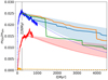 |
Fig. 1. Relative mass (μÖO ≡ mÖO/mdm) evolution of the Öpik-Oort cloud. Blue dots (top left) result from simulating 1000 Myr evolution of the Oort cloud for an isolated Solar System. Orange points (bottom) represent the formation of an Öpik-Oort cloud in a stellar cluster; no appreciable Oort cloud forms in these models. The red dots give the mass evolution of the Oort cloud if the Sun left the parent cluster at an age of 20 Myr. The dotted curves (blue, red, and orange) fit to the simulated data using a fast-rise-exponential-decay (see Sect:Fred), with trise = 10 Myr for the blue and orange curves, 80 Myr for the red curve, and all three curves have tdecay = 3500 Myr. The solid curves give the Öpik-Oort cloud mass-evolution for a star in a Galactic orbit for three independent calculations by Hanse et al. (2018). A similar mass evolution of the Öpik-Oort cloud was already calculated by Kaib & Quinn (2008, see their Fig. 7b). The large jumps in these curves result from encounters with other Galactic stars. The blue-shaded region shows the uncertainty interval derived from these calculations (Hanse et al. 2018). The red-shaded region provides the uncertainty interval of a similar analysis for a Solar System that left the parent cluster after 20 Myr. Both areas are bracketed by tdecay = 4000 Myr and tdecay = 13 000 Myr. The vertical black-dotted curve indicates the moment of reaching the maximum Oort-cloud mass for the isolated Solar System (see Sect:Methods). From this moment, Galactic erosion went on to dominate the Oort cloud’s evaporation. |
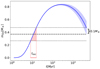 |
Fig. 2. Reconstruction of the time when the Sun left the parent cluster for a specific set of parameters. The dark blue curve shows the Öpik-Oort cloud’s mass-evolution, assuming it was born in isolation (fast-rise-exponential-decay function with a maximum mass of μÖO = 0.027, trise = 10 Myr, and tdecay = 7500 Myr, see Eq:FRED). The blue-shaded area gives the uncertainty of the Öpik-Oort cloud for tdecay = 5000 Myr to 10 000 Myr (see also fig:currentOCmass in the main paper). The dashed line indicates 0.38 M⊕ below the endpoint of the solid blue curve. The intersections between the dashed line and the solid blue curve (to the left) indicate the moment the Sun left the parent cluster at tesc = 12 ± 4 Myr. The horizontal dotted lines are identical to the dashed line, but present the extremes for the blue-shaded region; they define the uncertainty in tesc, indicated in red. |
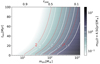 |
Fig. 3. Today’s Oort cloud mass (mÖO, shades) as a function of the planetesimal disk-mass (mdm) and the Sun’s escape time, tesc. Here, mdm is the leftover mass of the debris disk after the giant planets’ cores formed (here, the mass in planets’ cores is mpc). Along the top axis we express mdm in terms of the planet-formation efficiency, ϵpae ≡ mdm/(mdm + mpc). The curves indicate the current mass of the Öpik-Oort cloud (in units of M⊕) for a decay timescale, tdecay = 5000 Myr (white) and tdecay = 10 000 Myr (red). See also the color bar (to the right). Here, we calculated mÖO from the analytic model Eq:FRED presented in Sect:Fred (based on fig:OCGalacticOrbit). |
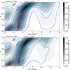 |
Fig. 4. Distribution of semimajor axis and eccentricity of the Solar System planetesimals. The distributions are presented at their peak, at the age of 226 Myr. The gray shades give the probability density function (linearly interpolated) for the Solar System that was ejected 20 Myr after the formation of the giant planets. The red curves indicate the influence of Earth (left, the dotted curve for reference), Jupiter (middle), and Neptune (rightmost curve). The two dotted curves around Neptune’s influence indicate the range within 5 Hill radii of Neptune. Top panel: Contours (same interpolation) give the probability density distribution for the Solar System that was isolated for its entire lifetime. Bottom panel: Contours (same interpolation and range) refer to the probability density distribution for the Solar System that remained in the cluster for its entire lifetime. |
A prolonged evolution in isolation or in a clustered environment also has consequences for near-Earth objects (NEOs). The number of NEOs at the moment the Oort cloud reaches its peak mass is typically five times higher in the models where the Sun escapes in 20 Myr compared to the Sun born in isolation. Such a higher local planetesimal density, as seen in Fig. 4, may have interesting consequences for the earliest cratering record of the inner planets and Moon (see also Pfalzner et al. 2024a,b).
4. Discussion
According to Hanse et al. (2018), Hands et al. (2019), the Sun accreted the Oort cloud from other stars. Such accretion can only be successful if other stars also have their own Oort clouds. However, since no Öpik-Oort cloud forms while a star is a cluster member, material exchange among stars is prevented. Some inner material with a ≲ 10 000 au and low eccentricities (e ≲ 0.9) can be exchanged (Jílková et al. 2016; Pfalzner et al. 2024b), but this material is easily lost again when accreted in wide a ≳ 10 000 au orbits. The Oort-Hills cloud (Breslau et al. 2017; Hands et al. 2019) and the detached population (Jílková et al. 2015), on the other hand, are quite likely to be rich in extra-solar planetesimals due to exchange of material during close encounters in the young cluster.
The recently discovered population of 92 planetesimals with a > 50 au (two of which display a ≳ 103 au) was found by the Horizon mission (Fraser et al. 2024) with an eccentricity of e = 0.61 ± 0.16 and inclination of i = 13.1 ° ±15.4°. Their orbits are inconsistent with a formation in situ and from being ejected by giant-planet migration (de Sousa Ribeiro et al. 2020), both of which predict planetesimals beyond 50 au to have low eccentricities and low inclinations in a narrow range. Their orbits are, however, consistent with external perturbations induced by passing stars, which naturally lead to a wide range in eccentricity and inclination, and with much higher values (Jílková et al. 2016; Hands et al. 2019; Pfalzner et al. 2024b).
Alternatively, part of the Oort cloud could be captured from free-floating debris in the parent cluster (Levison et al. 2010) or from freezing out planetesimals into bound pairs with the Sun, much in the same way wide binaries form (Moeckel & Clarke 2011) or planets are captured (Perets & Kouwenhoven 2012). The rate calculated through gas expulsion in the young cluster by (Levison et al. 2010) overestimates the efficiency of this process because of their assumed sudden (in 104 yr) removal of the primordial gas from the cluster central region. Recent calculations of cluster formation indicate that gas is ejected in much smaller quantities, more slowly, and coming from the cluster periphery, rather than from the center (Guszejnov et al. 2021; Polak et al. 2024a), in contrast to the assumptions adopted in Levison et al. (2010). The remaining capture rate in a cluster of N stars derived by Moeckel & Clarke (2011), Rozner & Perets (2023) gives only a small fraction of 0.03 to 0.06 and ∝1/N. Although the Sun and potentially each of the other N ∼ 3000 to 104 stars in the cluster have already lost a considerable portion (∼60%) of their planetesimals by the time the Sun escapes the cluster, the fraction of objects remaining bound to the escaping Sun would be only 10−4 to 10−5. This is substantially smaller than the fraction of native planetesimals that populate the Oort cloud (∼0.027).
5. Conclusions
The existence of a rich Öpik-Oort cloud can then only be reconciled with an early escape from the parent cluster, much earlier than expected based on the estimated lifetime of a virialized birth cluster, which easily exceeds 100 Myr (Portegies Zwart 2009; Portegies Zwart et al. 2010). If the Sun was ejected from the young cluster by a strong encounter, the Öpik-Oort cloud can only have formed after this event, and the majority of material must be native to the Solar System. The whole cluster likely dissolved quickly. Roughly 50 to 90 percent of the stars are born in non-virial or fractal-structured environments (Arnold et al. 2022) that experience violent relaxation in the first 10 Myr (Goodwin & Bastian 2006). Such a cluster dissolves shortly thereafter (Goodwin 2009), consistent with our estimated time spent in the clustered environment. For the Sun, we then favor a dense (half-mass density ≳103stars/pc3) non-virial birth environment.
It is challenging to derive a minimum amount of time the Sun has spent in the cluster, but it must have been a member long enough to experience a strong encounter, if only to truncate the circumstellar disk at the observed Kuiper cliff (at ∼50 au, de la Fuente Marcos & de la Fuente Marcos 2024; Pfalzner et al. 2024a) and to explain the hot trans-Neptunian population (Punzo et al. 2014; Fraser et al. 2024) or the irregular moons (Pfalzner et al. 2024b). In that case, the ≳50 au planetesimals were scattered in the last encounter to their current orbits, either originating from the Sun’s disk or being captured from the encountering star’s disk. An early escape also has consequences for the expected number and the proximity of supernovae in the infant Sun’s neighborhood. The first supernova typically happens between 8 and 10 Myr after the cluster’s birth (Portegies Zwart 2019). Such a nearby supernova could explain the Solar System’s abundance in terms of short-lived radionuclides (Arakawa & Kokubo 2023) and the observed ∼7° tilt in the ecliptic to the Sun’s equatorial plane (Portegies Zwart 2019). We expect that the birth cluster was non-virial, probably containing more stars than the hitherto estimated 2500 ± 500 stars (Portegies Zwart 2009; Higuchi & Kokubo 2015; Arakawa & Kokubo 2023). Finally, we assume the Sun left the nest within 20 Myr after the giant planets formed.
Data availability
This work is carried out using the Astronomical Multipurpose Software Environment (AMUSE). AMUSE is open source under the Apache-2.0 license, and the entire source code can be downloaded via https://github.com/amusecode/amuse. The simulations in this work were performed using AMUSE version v2024.6.0). We used the LonelyPlanets AMUSE script, which is open source under the Apache-2.0 license, and the entire source code can be downloaded via https://github.com/spzwart/LonelyPlanets
The simulation data, and specific scripts to generate the figures in this manuscript can be downloaded through FigShare at https://figshare.com/articles/preprint/Once_upon_a_time_in_the_Oort_cloud_when_did_the_Sun_Lost_its_Siblings/25744584?file = 49605921 (DOI: 10.21203/rs.3.rs-4257777/v1).
Acknowledgments
We thank Anthony Brown, Steven Rieder and Eiichiro Kokubo for discussions. Many of our calculations were performed on the two workstations of Ignas Snellen and Yamila Miguel; we thank their students for their patience. This work used the Dutch national e-infrastructure and in particular the Cartesius supercomputer with the support of the SURF Cooperative using grant numbers EINF-12718 and 2024.058. Considering the climate and energy consumption, we wish to report on the damage our work has done to the environment. The calculations have been running for about four months on dual 128-core Xeon-equipped workstations, totaling about 1024 core-days. Assuming a CPU consumption of 12 Watt h−1, the total energy is roughly 0.3 MWh. For an emission intensity of 0.283 kWh kg−1 (Wittmann et al. 2016), our calculations emitted 1 tonne CO2.
References
- Arakawa, S., & Kokubo, E. 2023, A&A, 670, A105 [NASA ADS] [CrossRef] [EDP Sciences] [Google Scholar]
- Arnold, B., Wright, N. J., & Parker, R. J. 2022, MNRAS, 515, 2266 [NASA ADS] [CrossRef] [Google Scholar]
- Batygin, K., Mardling, R. A., & Nesvorný, D. 2021, ApJ, 920, 148 [Google Scholar]
- Brasser, R. 2025, A&A, 694, A318 [NASA ADS] [CrossRef] [EDP Sciences] [Google Scholar]
- Brasser, R., Duncan, M. J., & Levison, H. F. 2006, Icarus, 184, 59 [NASA ADS] [CrossRef] [Google Scholar]
- Brasser, R., Duncan, M. J., & Levison, H. F. 2007, Icarus, 191, 413 [NASA ADS] [CrossRef] [Google Scholar]
- Brasser, R., Duncan, M. J., & Levison, H. F. 2008, Icarus, 196, 274 [Google Scholar]
- Breslau, A., Vincke, K., & Pfalzner, S. 2017, A&A, 599, A91 [NASA ADS] [CrossRef] [EDP Sciences] [Google Scholar]
- Cai, M. X., Portegies Zwart, S., Kouwenhoven, M. B. N., & Spurzem, R. 2019, MNRAS, 489, 4311 [NASA ADS] [CrossRef] [Google Scholar]
- de la Fuente Marcos, C., & de la Fuente Marcos, R. 2024, MNRAS, 527, L110 [Google Scholar]
- Desch, S. J. 2007, ApJ, 671, 878 [NASA ADS] [CrossRef] [Google Scholar]
- de Sousa Ribeiro, R., Morbidelli, A., Raymond, S. N., et al. 2020, Icarus, 339, 113605 [Google Scholar]
- Dones, L., Weissman, P. R., Levison, H. F., & Duncan, M. J. 2004, Oort cloud formation and dynamics, eds. M. C. Festou, H. U. Keller, & H. A. Weaver, 153 [Google Scholar]
- Duncan, M., Quinn, T., & Tremaine, S. 1987, AJ, 94, 1330 [Google Scholar]
- Emel’Yanenko, V. V., Asher, D. J., & Bailey, M. E. 2007, MNRAS, 381, 779 [Google Scholar]
- Fernandez, J. A. 1980, Icarus, 42, 406 [Google Scholar]
- Fernandez, J. A., & Ip, W. H. 1984, Icarus, 58, 109 [NASA ADS] [CrossRef] [Google Scholar]
- Fouchard, M., Emel’yanenko, V., & Higuchi, A. 2020, Celest. Mech. Dyn. Astron., 132, 43 [NASA ADS] [CrossRef] [Google Scholar]
- Francis, P. J. 2005, ApJ, 635, 1348 [NASA ADS] [CrossRef] [Google Scholar]
- Fraser, W. C., Porter, S. B., Peltier, L., et al. 2024, Planet. Sci. J., 5, 227 [Google Scholar]
- Fujii, M., Iwasawa, M., Funato, Y., & Makino, J. 2007, PASJ, 59, 1095 [NASA ADS] [Google Scholar]
- Goodwin, S. P. 2009, Ap&SS, 324, 259 [Google Scholar]
- Goodwin, S. P., & Bastian, N. 2006, MNRAS, 373, 752 [Google Scholar]
- Griveaud, P., Crida, A., Petit, A. C., Lega, E., & Morbidelli, A. 2024, A&A, 688, A202 [NASA ADS] [CrossRef] [EDP Sciences] [Google Scholar]
- Gurrutxaga, N., Johansen, A., Lambrechts, M., & Appelgren, J. 2024, A&A, 682, A43 [NASA ADS] [CrossRef] [EDP Sciences] [Google Scholar]
- Guszejnov, D., Grudić, M. Y., Hopkins, P. F., Offner, S. S. R., & Faucher-Giguère, C.-A. 2021, MNRAS, 502, 3646 [NASA ADS] [CrossRef] [Google Scholar]
- Hadden, S., & Tremaine, S. 2024, MNRAS, 527, 3054 [Google Scholar]
- Hands, T. O., Dehnen, W., Gration, A., Stadel, J., & Moore, B. 2019, MNRAS, 490, 21 [Google Scholar]
- Hanse, J., Jílková, L., Portegies Zwart, S. F., & Pelupessy, F. I. 2018, MNRAS, 473, 5432 [Google Scholar]
- Heisler, J., & Tremaine, S. 1986, Icarus, 65, 13 [CrossRef] [Google Scholar]
- Helled, R., Anderson, J. D., Podolak, M., & Schubert, G. 2011, ApJ, 726, 15 [Google Scholar]
- Higuchi, A., & Kokubo, E. 2015, AJ, 150, 26 [Google Scholar]
- Hills, J. G. 1981, AJ, 86, 1730 [CrossRef] [Google Scholar]
- Hut, P., & Tremaine, S. 1985, AJ, 90, 1548 [Google Scholar]
- Jänes, J., Pelupessy, I., & Portegies Zwart, S. 2014, A&A, 570, A20 [NASA ADS] [CrossRef] [EDP Sciences] [Google Scholar]
- Jílková, L., Portegies Zwart, S., Pijloo, T., & Hammer, M. 2015, MNRAS, 453, 3157 [Google Scholar]
- Jílková, L., Hamers, A., Hammer, M., & Portegies Zwart, S. 2016, MNRAS, 457, 4218 [Google Scholar]
- Kaib, N. A., & Quinn, T. 2008, Icarus, 197, 221 [NASA ADS] [CrossRef] [Google Scholar]
- Kaib, N. A., & Volk, K. 2022, ArXiv e-prints [arXiv:2206.00010] [Google Scholar]
- Kokubo, E., & Ida, S. 1998, Icarus, 131, 171 [Google Scholar]
- Levison, H. F., Duncan, M. J., Brasser, R., & Kaufmann, D. E. 2010, Science, 329, 187 [NASA ADS] [CrossRef] [Google Scholar]
- Liu, B., Raymond, S. N., & Jacobson, S. A. 2022, Nature, 604, 643 [NASA ADS] [CrossRef] [Google Scholar]
- Makino, J., & Aarseth, S. J. 1992, PASJ, 44, 141 [NASA ADS] [Google Scholar]
- Marochnik, L. S., Mukhin, L. M., & Sagdeev, R. Z. 1988, Science, 242, 547 [Google Scholar]
- Meech, K. J., Weryk, R., Micheli, M., et al. 2017, Nature, 552, 378 [Google Scholar]
- Moeckel, N., & Clarke, C. J. 2011, MNRAS, 415, 1179 [NASA ADS] [CrossRef] [Google Scholar]
- Nesvorný, D., & Morbidelli, A. 2012, AJ, 144, 117 [Google Scholar]
- Oort, J. H. 1950, Bul. Astron. Inst. Neth., 11, 91 [Google Scholar]
- Öpik, E. 1932, Proc. Am. Academy Arts Sci., 67, 169 [Google Scholar]
- Pelupessy, F. I., Jänes, J., & Portegies Zwart, S. 2012, New Astron., 17, 711 [Google Scholar]
- Perets, H. B., & Kouwenhoven, M. B. N. 2012, ApJ, 750, 83 [NASA ADS] [CrossRef] [Google Scholar]
- Pfalzner, S., Govind, A., & Portegies Zwart, S. 2024a, Nat. Astron., 8, 1380 [NASA ADS] [CrossRef] [Google Scholar]
- Pfalzner, S., Govind, A., & Wagner, F. W. 2024b, ApJ, 972, L21 [Google Scholar]
- Polak, B., Mac Low, M.-M., Klessen, R. S., et al. 2024a, A&A, 690, A207 [NASA ADS] [CrossRef] [EDP Sciences] [Google Scholar]
- Polak, B., Mac Low, M.-M., Klessen, R. S., et al. 2024b, A&A, 690, A94 [NASA ADS] [CrossRef] [EDP Sciences] [Google Scholar]
- Portegies Zwart, S. F. 2009, ApJ, 696, L13 [NASA ADS] [CrossRef] [Google Scholar]
- Portegies Zwart, S. 2019, A&A, 622, A69 [NASA ADS] [CrossRef] [EDP Sciences] [Google Scholar]
- Portegies Zwart, S. F., & Jílková, L. 2015, MNRAS, 451, 144 [Google Scholar]
- Portegies Zwart, S., & McMillan, S. 2018, Astrophysical Recipes; The art of AMUSE (Bristol, UK: IOP Publishing) [Google Scholar]
- Portegies Zwart, S. F., McMillan, S. L. W., & Gieles, M. 2010, ARA&A, 48, 431 [NASA ADS] [CrossRef] [Google Scholar]
- Portegies Zwart, S., Pelupessy, I., Martínez-Barbosa, C., van Elteren, A., & McMillan, S. 2020, Commun. Nonlinear Sci. Numer. Simul., 85, 105240 [Google Scholar]
- Punzo, D., Capuzzo-Dolcetta, R., & Portegies Zwart, S. 2014, MNRAS, 444, 2808 [Google Scholar]
- Rozner, M., & Perets, H. B. 2023, ApJ, 955, 134 [Google Scholar]
- Smoluchowski, R., & Torbett, M. 1984, Nature, 311, 38 [Google Scholar]
- Stock, K., Cai, M. X., Spurzem, R., Kouwenhoven, M. B. N., & Portegies Zwart, S. 2020, MNRAS, 497, 1807 [Google Scholar]
- Strang, G. 1968, SIAM J. Numerical Anal., 5, 506 [Google Scholar]
- Toomre, A., & Toomre, J. 1972, ApJ, 178, 623 [Google Scholar]
- Wahl, S. M., Hubbard, W. B., Militzer, B., et al. 2017, Geophys. Res. Lett., 44, 4649 [CrossRef] [Google Scholar]
- Wiegert, P., & Tremaine, S. 1999, Icarus, 137, 84 [Google Scholar]
- Wilhelm, M. J. C., Portegies Zwart, S., Cournoyer-Cloutier, C., et al. 2023, MNRAS, 520, 5331 [NASA ADS] [CrossRef] [Google Scholar]
- Wittmann, M., Hager, G., Zeiser, T., Treibig, J., & Wellein, G. 2016, Concurrency and Computation: Practice and Experience, 28, 2295 [CrossRef] [Google Scholar]
- Yabushita, S. 1979, MNRAS, 187, 445 [Google Scholar]
Appendix A: Isolated planetary systems
We simulate isolated planetary systems and those perturbed in a clustered environment using the AMUSE framework. AMUSE (Portegies Zwart & McMillan 2018) is a high-performance software instrument for simulating four fundamental physics domains: gravity, hydrodynamics, stellar evolution, and radiative transfer. It can be used for a wide variety of applications. The various codes that solve for these domains are interchangeable and can run concurrently on different resolutions and scales.
To simulate an isolated planetary system, we started with the Sun and the four giant planets using ephemerides at Julian date 2588106.62749, with their current masses. We subsequently added a population of minor bodies in the ecliptic with circular (e ≤ 0.01) orbits between 1 au and 42 au around the Sun (Marochnik et al. 1988; Gurrutxaga et al. 2024). The minor bodies have no mass and no size. The surface density of the disk follows a −1.5 power-law and has a Toomre Q-parameter of 1.0 (Toomre & Toomre 1972). We generated planetary systems using the AMUSE routine ProtoPlanetaryDisk. We rotated the Solar system (planets and planetesimals) along the y-axis by 60.2° and put it in a circular orbit in the Galactic plane at a distance of 8.5 kpc along the x-axis. We then moved the center of mass of the simulated Solar system by 7.5 pc in the Galactic z-coordinate, and give it an additional velocity of 10.1 km/s towards the Galactic center. This places the Solar System in a slightly elliptical and inclined orbit in the Galactic potential, with the Solar System’s ecliptic inclined by about 60°. We adopted the simple Galactic potential presented in (Portegies Zwart & McMillan 2018).
The planetesimals in our calculations are massless. Still, we can consider our results in light of the planet formation efficiency. For this estimate, we focused on the mass in rocky cores of the giant planets. Jupiter’s core mass has an upper limit of 45 M⊕ (Wahl et al. 2017), for Saturn we adopted 25 M⊕ (Gurrutxaga et al. 2024), 13 M⊕ for Uranus and 15.5 M⊕ for Neptune (Desch 2007; Helled et al. 2011). The upper limit to the mass in a giant planet core is then mpc ≃ 98.5 M⊕. The original mass of the disk in solids, before the planets formed must then have been at least 98.5 M⊕ plus the current mass of minor planets and planetesimals give a minimum disk mass of ∼100 M⊕. The mass scaling from test particles to appropriate mass units is realized by adopting an initial disk mass, as presented in fig:currentOCmass.
The dynamical evolution of the planetary systems was performed with the direct N-body code Huayno, using the drift-kick-drift integrator with time step parameter η = 0.03. The dynamics of the Solar System and the Galaxy are coupled using the bridge method (Fujii et al. 2007) with a time-step of 0.01 Myr. This is a conservative choice considering the static nature of the background potential, but it allows us to use the same time step when including stellar encounters, which require a high time resolution. A bridge time step of 0.01Myr corresponds to the period of a circular orbit at about 460au, which is more than a factor 60 shorted than inner edge of the Öpik-Oort cloud boundary at 30 000 au.
Appendix B: Oort cloud formation in isolation
We ran 27 simulations with 4 planets and 103 planetesimals. In principle, we could have performed a single simulation with 27 000 planetesimals at the same cost, but we now can address the stochasticity in the results due to the chaotic dynamics of the planetary system, and we adopt the same planetary systems in a dynamical environment, as we discuss further down.
For each simulation, we identified various dynamical classes. Rather than listing the entire procedure for identifying minor bodies, we provide the selection criteria for the various Oort-cloud objects and the remaining trans-Neptunians (which includes the various Kuiper-belt families).
The orbital elements were calculated using a Kepler solver in the Solar System’s barycenter. The procedure for identifying dynamical classes is as follows:
-
First, classify the bound planetesimals (with e < 1).
-
Then we select those with pericenter distance a(1 − e) > 5 Hill radii further away from the Sun than the planet Neptune.
-
Those with a ≥ 30 000 au populate the Öpik-Oort cloud.
-
The remaining planetesimals with a ≥ 1 000 au populate the Oort-Hills cloud.
-
the left over (detached but with a < 1 000 au) are the detached objects.
-
We adopted an inner edge of the Öpik-Oort cloud of rinner = 30 000 au; however, based on Fig. 4 of the main paper, we could consider an inner limit around 10 000 au to be more distinctive, as this is also around the region beyond which the Galactic tidal field starts to become important.
Once classified, we can describe the evolution of the various detached populations. We started by measuring the time and number at the peak of the Öpik-Oort cloud in each of our simulations. The results are presented in Fig. B.1, showing the time and maximum of the Oort cloud in each of the 27 simulation and the statistical average.
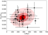 |
Fig. B.1. Peak in the relative mass of the Öpik-Oort cloud (μÖO) for the isolated Solar System. The black bullet points represent the measured maximum mass of the Öpik-Oort cloud, with 1 standard deviation uncertainty, measured at the time the maximum Öpik-Oort cloud mass is reached. The shaded areas show the uncertainty obtained from 27 calculations centered on the global mean with the error ellipse for 0.5 (darkest shade red), 1.0, and 2.0 (lightest shade) standard deviations. A least-squares fit of a linear function to the data does not give a significant result. The geometric mean of the 27 bullet points is at a mass of mdm = 0.027 ± 0.006, at an age of 226 ± 24 Myr. |
Appendix C: Numerical noise and chaos
In principle, the planets in each of our isolated systems should evolve identically because they start with identical initial realization for the Sun and planets, whereas the planetesimals, which are treated as test particles, have orbits randomly selected from the initial conditions. Integrating these systems causes variations in the round-off at the least significant digit. This round-off drives chaos in our calculations, causing the orbital evolution of the planets to be different for different planetary systems. To validate our results in terms of its chaotic behavior of the system, and to ensure that the results are not driven by the chaotic nature of the system, we calculate the largest positive Lyapunov timescale, tLy, for each of the 351 unique pairs of planetary systems.
The Lyapunov timescale is calculated by fitting the growth of the difference between the normalized orbital semimajor axes of the four planets. Fitting an exponential relation gives an estimate for the relative growth of numerical errors due to round-off, and the Lyapunov timescale is its reciprocal.
We find a mean Lyapunov timescale of ⟨tLy⟩ = 800 ± 230 Myr, with a tail to tLy = 4000 Myr containing ∼20% of the cases. The Lyapunov timescale is of the order of our calculation time (1000 Myr), indicating that our calculations are indeed chaotic, as expected, but this has not affected the results. Upon inspection of the planets’ orbital parameters at the end of the simulations, we find slight variations of the order of ∼0.4% in orbital separation. We consider these small compared to the variations in orbital separation needed to affect the results, which would be around an order of magnitude larger.
Appendix D: Planetary system in a stellar cluster
Planetary systems in a stellar cluster are simulated in two stages using the LonelyPlanets AMUSE script. This new implementation of the method, introduced in (Cai et al. 2019), is now independent of the adopted N-body integrator, and it is available at github1. The new LonelyPlanet script includes stellar evolution, collisions, and a semi-analytic background Galactic potential.
Integrating a star cluster, including planetary systems, is impractically expensive in terms of computer time. In LonelyPlanets, we reduce these costs through a two-stage divide-and-conquer strategy (Cai et al. 2019; Stock et al. 2020). In stage one, we simulate a dynamical evolution and stellar evolution of a cluster of N stars in the Galactic potential: In stage two, we integrate the planetary systems with only the nearest perturbing cluster members. This strategy easily saves a factor of 104 in computer time.
In stage one, the stars’ motion equations in the cluster are integrated using an N-body code dedicated to cluster dynamics. For this work, we opted for the 4th-order Hermite predictor-corrector scheme (Makino & Aarseth 1992) Ph4 (Portegies Zwart & McMillan 2018). The coupling of the direct N-body code for the cluster dynamics and the semi-analytic background potential of the Galaxy is realized using bridge (Fujii et al. 2007). Bridge is a non-intrusive hierarchical code-coupling strategy based on solving the combined Hamiltonian as two separate parts using Strang splitting (Strang 1968). Both parts are later combined to form a homogeneous and self-consistent solution using a kick-drift-kick scheme, as was demonstrated in (Portegies Zwart et al. 2020).
While integrating the cluster, we keep track of the Ncc = 6 closest encountering stars and the strongest perturbers for a subset of 27 selected stars. We store the encounter information between selected stars and perturbers at a fine time resolution of 0.01 Myr. Stage one is illustrated in Fig. D.1 where we show the orbit of one selected star in a cluster of 103 stars over 7 Myr. The right-hand panel shows the distance for the selected star to its Ncc = 6 nearest neighbors (which includes the 3 strongest perturbers). The shaded regions in the right-hand panel indicate when the selected star is strongly perturbed. In this particular case, the selected star escapes the cluster after a particularly strong encounter at ∼5.7 Myr.
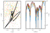 |
Fig. D.1. Initial cluster (left: rainbow colors and size represent stellar mass) and the orbit of a randomly selected star evolved for 7 Myr (black curve). Circles along the orbit indicate moments of close approach. The right-hand panel shows the distance to the six nearest neighbors as the selected star orbits the cluster. The gray shaded area indicates when another star approaches within 104 au. |
In stage two, each of the stars acquires a system of Np = 4 planets and Na = 1000 planetesimals. The planetesimals are test particles; they do not feel each other’s gravity and do not exert a force on any of the planets or stars. We integrate the orbits of the planets and planetesimals together with the earlier stored neighboring stars, replenishing this population every 0.01 Myr. In some sense, we reconstruct the perturbed star’s dynamical history while integrating it including its planetary system. Each planetary system, including its perturbers, is integrated using the symplectic coupled-components drift-kick-drift algorithm Huayno (Pelupessy et al. 2012; Jänes et al. 2014).
Stage two is illustrated in Fig. D.2 where we show the evolution of the orbits of six planets around the selected star. The choice of the number of planets is arbitrary; it just shows the workings of the code. The encounter that ejected the star from the cluster (at ∼5.7 Myr) also caused a variation in the semimajor axis and eccentricity in the outermost planets. This perturbation is propagated to the inner planets’ orbits on a secular timescale.
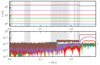 |
Fig. D.2. Evolution of the orbital separation (top) and eccentricity (bottom) for the selected star in fig. D.1, but now with six planets between 1 au and 180 au according to an Oligarchic planet-formation model (Kokubo & Ida 1998). The planetary system was integrated for 7 Myr, while the 6 nearest stars were taken into account in the gray-shaded areas. The initial planetary system would have been stable if it evolved in isolation, but the perturbations caused several planets to change their orbits considerably. Most noticeable is the high increase in eccentricity to 0.31 of the outermost planet due to the encounter that kicked the star from the cluster (see Fig. D.1). An earlier encounter at 3.8 Myr already affected the outer planet’s orbit. |
Integrating the planetary system requires  operations per time step. Once the star escapes the cluster, its planetary system is unlikely to be perturbed by nearby stars, but it remains affected by the Galactic tidal field. The isolated planetary system is integrated by a symplectic integrator, which bridges with the semi-analytic Galactic potential.
Integrating the cluster of 1000 stars and 27 planetary systems for 1000 Myr using a direct (symplectic) method would require some 1.7 ⋅ 1021 flops (28108 stars, planets, and planetesimals in total integrated with a 1 day time step, assuming 60 operations per force calculation). Such a calculation would cost about two weeks on a PetaFlop-scale computer. In LonelyPlanets the same calculations can be done in only 6 ⋅ 1011 operations for the cluster simulation and 1.7 ⋅ 1015 (about two weeks on a 128-core workstation) operations for each of the planetary systems. The speedup due to LonelyPlanets then amounts to a factor of ≳104 compared to conventionally integrating the cluster with planets.
We performed several calculations of planetary systems in stellar clusters. We adopted the same 27 planetary systems every time but varied the cluster parameters.
We adopted virialized Plummer spheres with 100 to 6000 stars from a Salpeter mass function between 0.1 M⊙ and 100 M⊙ with virial radii of 0.5 pc, 1.0 pc and 1.5 pc. These clusters cover a wide range of initial half-mass densities from 3.7 pc−3 to 6000 pc−3. We also performed simulations with a more complex initial realization in which we adopted the results from a hydrodynamics molecular cloud collapse simulation until the gas was depleted (Wilhelm et al. 2023; Polak et al. 2024a,b).
After initializing the cluster stars, we select 27 stars with a mass closest to 1 M⊙ in each of these initial realizations and turn them into 1 M⊙ stars. After this we correct for the mass change by rescaling the system to virial equilibrium. We note that we did not rescale the clusters resulting from the hydrodynamical simulation, as it was initially not in virial equilibrium.
We continue each simulation to 1000 Myr, but stop integrating each Solar-equivalent system after losing a planet or if the number of planetesimals drops below 50. Many of the planetary systems were destroyed before that time, particularly in those runs with a high stellar density. Eventually, we analyze the data for the surviving planetary systems.
The initial stellar distribution did not make a statistically significant difference for the surviving planetesimal orbital distributions in the Öpik-Oort cloud. The resulting mass evolution of the Öpik-Oort cloud, is summarized in the main paper Fig. 1. In all the simulations, the formation process of an Öpik-Oort cloud turns out to be too fragile to survive a long exposure in a clustered environment.
Appendix E: Further analysis on the growth and erosion of an Oort cloud
Ideally, we would like to infer the initial Oort-cloud mass by calculating backward in time in order to reconstruct when the Sun left the parent cluster. Since this inversion problem is not possible, we fit the measured Oort-cloud mass evolution and invert the fitted curve. We fit a fast-rise-exponential-decay (FRED) function of the form
 (E.1)
(E.1)
to the mass evolution of the Oort cloud. The three free parameters in this function includes the proportionality constant μÖO, and the two timescales, trise and tdecay. The mass of the Oort cloud then peaks at  . We fitted on the accumulated data for all 27 runs (see Fig. E.1). The Öpik-Oort cloud is best described with a FRED with a relative peak value of μÖO = 0.027, trise = 10 Myr, and tdecay between 4 000 Myr and 13 000 Myr, whereas for Oort-Hills cloud μOH = 0.027, trise = 80 Myr for a similar decay timescale. The resulting fits for the Öpik-Oort cloud are presented in the main paper fig:OCGalacticOrbit, Fig. 2, and Fig. E.1. In Fig. E.1 we present the mass evolution of various Oort cloud populations as a function of time. The Öpik-Oort cloud for both simulations are over-plotted with the fit.
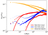 |
Fig. E.1. Relative mass evolution of the Oort cloud and detached population. For isolated clusters the mass evolution of the Öpik-Oort cloud, Oort-Hills cloud, and the detached populations are given by the upper red, blue and orange symbols, respectively. The triangles give the mass evolution in the simulation where the Solar System left the cluster 20 Myr after the formation of the giant planets, the bullets for the isolated Solar System. Here we adopted the inner Öpik-Oort cloud boundary of rinner = 30 000 au. The red symbols are identical to the blue and red dots in the main paper’s Fig. 1. The two solid red curves represent the fits to the two Öpik-Oort cloud populations. |
Our adopted choice of the inner boundary for the Öpik-Oort cloud of rinner = 30 000 au is somewhat arbitrary. We therefore fit μÖO and trise as a function of this inner boundary. The values for mÖO and trise depend on the inner edge rinner as follows
 (E.2)
(E.2)
The rise-time depends on the Öpik-Oort cloud inner edge as follows
 (E.3)
(E.3)
The Öpik-Oort cloud in the isolated Solar System, starts growing from the start of the simulation. We anticipate that our starting point coincides with the moment the giant planets stop migrating and have reached their current mass. In the clustered environment, the Öpik-Oort cloud can only start to form after the Sun escapes and becomes isolated, (in the simulation this happens at an age of 20 Myr). This moment is visible in the dip in the formation of the Oort-Hills cloud, of Fig. E.1 around 20 Myr (see blue triangles). In contrast to the Öpik-Oort cloud The Oort-Hills cloud already starts to be populated while the Solar System is a cluster member. The exchange of planetesimals between the Oort-Hills cloud (blue) and the detached population (yellow) proceeds differently if the Solar System is born in isolation (bullets in Fig. E.1) or in a clustered environment (triangles).
Finally, in Fig. E.2 we present the orbital distribution (semimajor axis and eccentricity) of the planetesimals that remained in the Solar System at an age of 1 Gyr. The shaded regions indicate the density distribution if the Solar System escapes the cluster at the age of 20 Myr. The contours refer to the isolated Solar System.
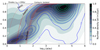 |
Fig. E.2. Semimajor axis versus eccentricity of the Solar System planetesimals at the age of 1000 Myr for the isolated case (contours), and if the Solar System left the cluster at an age of 20 Myr (shades). Both distributions are normalized independently to the maximum value with 10 equally-spaced contour levels each. In Fig. 4 (main paper), we present the results of the same simulations but at an age of 226 Myr. |
All Figures
|
Fig. 1. Relative mass (μÖO ≡ mÖO/mdm) evolution of the Öpik-Oort cloud. Blue dots (top left) result from simulating 1000 Myr evolution of the Oort cloud for an isolated Solar System. Orange points (bottom) represent the formation of an Öpik-Oort cloud in a stellar cluster; no appreciable Oort cloud forms in these models. The red dots give the mass evolution of the Oort cloud if the Sun left the parent cluster at an age of 20 Myr. The dotted curves (blue, red, and orange) fit to the simulated data using a fast-rise-exponential-decay (see Sect:Fred), with trise = 10 Myr for the blue and orange curves, 80 Myr for the red curve, and all three curves have tdecay = 3500 Myr. The solid curves give the Öpik-Oort cloud mass-evolution for a star in a Galactic orbit for three independent calculations by Hanse et al. (2018). A similar mass evolution of the Öpik-Oort cloud was already calculated by Kaib & Quinn (2008, see their Fig. 7b). The large jumps in these curves result from encounters with other Galactic stars. The blue-shaded region shows the uncertainty interval derived from these calculations (Hanse et al. 2018). The red-shaded region provides the uncertainty interval of a similar analysis for a Solar System that left the parent cluster after 20 Myr. Both areas are bracketed by tdecay = 4000 Myr and tdecay = 13 000 Myr. The vertical black-dotted curve indicates the moment of reaching the maximum Oort-cloud mass for the isolated Solar System (see Sect:Methods). From this moment, Galactic erosion went on to dominate the Oort cloud’s evaporation. |
| In the text | |
|
Fig. 2. Reconstruction of the time when the Sun left the parent cluster for a specific set of parameters. The dark blue curve shows the Öpik-Oort cloud’s mass-evolution, assuming it was born in isolation (fast-rise-exponential-decay function with a maximum mass of μÖO = 0.027, trise = 10 Myr, and tdecay = 7500 Myr, see Eq:FRED). The blue-shaded area gives the uncertainty of the Öpik-Oort cloud for tdecay = 5000 Myr to 10 000 Myr (see also fig:currentOCmass in the main paper). The dashed line indicates 0.38 M⊕ below the endpoint of the solid blue curve. The intersections between the dashed line and the solid blue curve (to the left) indicate the moment the Sun left the parent cluster at tesc = 12 ± 4 Myr. The horizontal dotted lines are identical to the dashed line, but present the extremes for the blue-shaded region; they define the uncertainty in tesc, indicated in red. |
| In the text | |
|
Fig. 3. Today’s Oort cloud mass (mÖO, shades) as a function of the planetesimal disk-mass (mdm) and the Sun’s escape time, tesc. Here, mdm is the leftover mass of the debris disk after the giant planets’ cores formed (here, the mass in planets’ cores is mpc). Along the top axis we express mdm in terms of the planet-formation efficiency, ϵpae ≡ mdm/(mdm + mpc). The curves indicate the current mass of the Öpik-Oort cloud (in units of M⊕) for a decay timescale, tdecay = 5000 Myr (white) and tdecay = 10 000 Myr (red). See also the color bar (to the right). Here, we calculated mÖO from the analytic model Eq:FRED presented in Sect:Fred (based on fig:OCGalacticOrbit). |
| In the text | |
|
Fig. 4. Distribution of semimajor axis and eccentricity of the Solar System planetesimals. The distributions are presented at their peak, at the age of 226 Myr. The gray shades give the probability density function (linearly interpolated) for the Solar System that was ejected 20 Myr after the formation of the giant planets. The red curves indicate the influence of Earth (left, the dotted curve for reference), Jupiter (middle), and Neptune (rightmost curve). The two dotted curves around Neptune’s influence indicate the range within 5 Hill radii of Neptune. Top panel: Contours (same interpolation) give the probability density distribution for the Solar System that was isolated for its entire lifetime. Bottom panel: Contours (same interpolation and range) refer to the probability density distribution for the Solar System that remained in the cluster for its entire lifetime. |
| In the text | |
|
Fig. B.1. Peak in the relative mass of the Öpik-Oort cloud (μÖO) for the isolated Solar System. The black bullet points represent the measured maximum mass of the Öpik-Oort cloud, with 1 standard deviation uncertainty, measured at the time the maximum Öpik-Oort cloud mass is reached. The shaded areas show the uncertainty obtained from 27 calculations centered on the global mean with the error ellipse for 0.5 (darkest shade red), 1.0, and 2.0 (lightest shade) standard deviations. A least-squares fit of a linear function to the data does not give a significant result. The geometric mean of the 27 bullet points is at a mass of mdm = 0.027 ± 0.006, at an age of 226 ± 24 Myr. |
| In the text | |
|
Fig. D.1. Initial cluster (left: rainbow colors and size represent stellar mass) and the orbit of a randomly selected star evolved for 7 Myr (black curve). Circles along the orbit indicate moments of close approach. The right-hand panel shows the distance to the six nearest neighbors as the selected star orbits the cluster. The gray shaded area indicates when another star approaches within 104 au. |
| In the text | |
|
Fig. D.2. Evolution of the orbital separation (top) and eccentricity (bottom) for the selected star in fig. D.1, but now with six planets between 1 au and 180 au according to an Oligarchic planet-formation model (Kokubo & Ida 1998). The planetary system was integrated for 7 Myr, while the 6 nearest stars were taken into account in the gray-shaded areas. The initial planetary system would have been stable if it evolved in isolation, but the perturbations caused several planets to change their orbits considerably. Most noticeable is the high increase in eccentricity to 0.31 of the outermost planet due to the encounter that kicked the star from the cluster (see Fig. D.1). An earlier encounter at 3.8 Myr already affected the outer planet’s orbit. |
| In the text | |
|
Fig. E.1. Relative mass evolution of the Oort cloud and detached population. For isolated clusters the mass evolution of the Öpik-Oort cloud, Oort-Hills cloud, and the detached populations are given by the upper red, blue and orange symbols, respectively. The triangles give the mass evolution in the simulation where the Solar System left the cluster 20 Myr after the formation of the giant planets, the bullets for the isolated Solar System. Here we adopted the inner Öpik-Oort cloud boundary of rinner = 30 000 au. The red symbols are identical to the blue and red dots in the main paper’s Fig. 1. The two solid red curves represent the fits to the two Öpik-Oort cloud populations. |
| In the text | |
|
Fig. E.2. Semimajor axis versus eccentricity of the Solar System planetesimals at the age of 1000 Myr for the isolated case (contours), and if the Solar System left the cluster at an age of 20 Myr (shades). Both distributions are normalized independently to the maximum value with 10 equally-spaced contour levels each. In Fig. 4 (main paper), we present the results of the same simulations but at an age of 226 Myr. |
| In the text | |
Current usage metrics show cumulative count of Article Views (full-text article views including HTML views, PDF and ePub downloads, according to the available data) and Abstracts Views on Vision4Press platform.
Data correspond to usage on the plateform after 2015. The current usage metrics is available 48-96 hours after online publication and is updated daily on week days.
Initial download of the metrics may take a while.