| Issue |
A&A
Volume 652, August 2021
|
|
|---|---|---|
| Article Number | A94 | |
| Number of page(s) | 17 | |
| Section | Cosmology (including clusters of galaxies) | |
| DOI | https://doi.org/10.1051/0004-6361/202039999 | |
| Published online | 17 August 2021 | |
Evolution of skewness and kurtosis of cosmic density fields
1
Tartu Observatory, University of Tartu, 61602 Tõravere, Estonia
e-mail: jaan.einasto@ut.ee
2
ICRANet, Piazza della Repubblica 10, 65122 Pescara, Italy
3
Estonian Academy of Sciences, 10130 Tallinn, Estonia
4
Astronomy Department, New Mexico State University, Las Cruces, NM 88003, USA
5
Department of Astronomy, University of Virginia, Charlottesville, VA 22904, USA
6
National Institute of Chemical Physics and Biophysics, Tallinn 10143, Estonia
Received:
26
November
2020
Accepted:
25
June
2021
Aims. We investigate the evolution of the one-point probability distribution function (PDF) of the dark matter density field and the evolution of its moments for fluctuations that are Gaussian in the linear regime.
Methods. We performed numerical simulations of the evolution of the cosmic web for the conventional ΛCDM model. The simulations covered a wide range of box sizes L = 256 − 4000 h−1 Mpc, mass, and force resolutions, and epochs from very early moments z = 30 to the present moment z = 0. We calculated density fields with various smoothing lengths to determine the dependence of the density field on the smoothing scale. We calculated the PDF and its moments variance, skewness, and kurtosis. We determined the dependence of these parameters on the evolutionary epoch z, on the smoothing length Rt, and on the rms deviation of the density field σ using a cubic-cell and top-hat smoothing with kernels 0.4 h−1 Mpc ≤ Rt ≤ 32 h−1 Mpc.
Results. We focus on the third (skewness S) and fourth (kurtosis K) moments of the distribution functions: their dependence on the smoothing scale Rt, the amplitude of the fluctuations σ, and the redshift z. Moments S and K, calculated for density fields at different cosmic epochs and smoothed with various scales, characterise the evolution of different structures of the web. Moments calculated with small-scale smoothing (Rt ≈ (1 − 4) h−1 Mpc) characterise the evolution of the web on cluster-type scales. Moments found with strong smoothing (Rt ≳ (5 − 15) h−1 Mpc) describe the evolution of the web on supercluster scales. During the evolution, the reduced skewness S3 = S/σ and reduced kurtosis S4 = K/σ2 present a complex behaviour: at a fixed redshift, curves of S3(σ) and S4(σ) steeply increase with σ at σ ≲ 1 and then flatten out and become constant at σ ≳ 2. When we fixed the smoothing scale Rt, the curves at large σ started to gradually decline after reaching the maximum at σ ≈ 2. We provide accurate fits for the evolution of S3, 4(σ, z). Skewness and kurtosis approach constant levels at early epochs S3(σ)≈3 and S4(σ)≈15.
Conclusions. Most of the statistics of dark matter clustering (e.g. halo mass function or concentration-mass relation) are nearly universal: they mostly depend on the σ with a relatively modest correction to apparent dependence on the redshift. We find just the opposite for skewness and kurtosis: the dependence of the moments on the evolutionary epoch z and smoothing length Rt is very different. Together, they uniquely determine the evolution of S3, 4(σ). The evolution of S3 and S4 cannot be described by current theoretical approximations. The often used lognormal distribution function for the PDF fails to even qualitatively explain the shape and evolution of S3 and S4.
Key words: large-scale structure of Universe / dark matter / cosmology: theory / methods: numerical
© ESO 2021
1. Introduction
According to the currently accepted cosmological paradigm, the evolution of the structure in the Universe began from small perturbations that were created during the epoch of inflation. The structure evolved by gravitational amplification to form the cosmic web that is observed now. It is also accepted that initial density fluctuations were random (but correlated) and had a Gaussian distribution. The Gaussian random field is symmetrical around the mean density, that is, positive and negative deviations from the mean density are equally probable. On the other hand, it is well known that the current density field of the cosmic web is highly asymmetric: positive density departures from the mean density can be very strong, while the negative deviations are restricted by the condition that the density cannot be negative. The asymmetry of the density field can be studied with a one-point probability distribution function (PDF) of the density field and its moments.
There are different ways of studying the properties of PDFs. Analytical methods are one approach (Peebles 1980; Bernardeau & Kofman 1995; Bernardeau et al. 2002). In this case, the PDF is modelled theoretically using cosmological perturbation theory (PT), which allows calculating the PDF and its moments variance, skewness, and kurtosis. The basic elements of the cosmological PT and its applications were discussed in detail by Peebles (1980), Bernardeau et al. (2002), and Szapudi (2009). Another possibility is calculating the evolution of the PDF numerically using N-body simulations. For early studies, see Kofman et al. (1992, 1994).
The asymmetry and flatness of the PDF are measured by the third (skewness S) and fourth (kurtosis K) moments of the distribution functions. The moments are the most simple forms of the three-point and four-point correlation functions, and they therefore cannot be reduced to second-order statistics such as the correlation function or the power spectrum. In mathematical statistics, skewness and kurtosis of a random variable are defined as dimensionless parameters and can be called mathematical skewness S and mathematical kurtosis K. They change during the evolution and can be used to characterise the evolution. In cosmology, there is a tradition to define skewness and kurtosis in a different way. These skewness and kurtosis parameters are called reduced (Lahav et al. 1993). To emphasise the difference between mathematical and cosmological terminology, we mostly use the term “cosmological”. Early studies suggested that during the evolution, cosmological skewness S3 and cosmological kurtosis S4 remained approximately constant and that they characterise the general properties of the model of the universe (Peebles 1980).
Simple relations exist between mathematical and cosmological parameters. The skewness is S(σ) = S3 × σ, and the kurtosis is K(σ) = S4 × σ2, where σ is the standard deviation of fluctuations of the density field. The initial density field that is generated during the inflation must have a density fluctuation with finite non-zero amplitude, σ > 0. Moreover, if initial fluctuations were Gaussian, then they should be symmetrical. Thus the question is how the asymmetry in the density distribution forms and evolves.
The tradition of quantifying the moments of the PDF follows Peebles (1980). Based on the linear PT, Peebles found that for the Einstein-de Sitter model with Ω = 1, the cosmological skewness has the value S3 = 34/7. Later studies showed that S3 also depends on the effective index n of the power spectrum, P(k)∝kn, as well as on the smoothing length R (Bouchet & Hernquist 1992; Bouchet et al. 1992; Juszkiewicz et al. 1993; Bernardeau 1994). Subsequent studies of the PDF and its moments have confirmed and extended these results; see for example Catelan & Moscardini (1994), Bernardeau & Kofman (1995), Juszkiewicz et al. (1995), Lokas et al. (1995), Gaztanaga & Bernardeau (1998), Gaztañaga et al. (2000), Kayo et al. (2001), and Uhlemann et al. (2017). These studies were theoretical and used various methods of the perturbation theory to follow the evolution of PDFs of the density field and its moments.
Various theoretical approximations were suggested to determine the values of cosmological skewness and kurtosis parameters. Bernardeau & Kofman (1995) listed in their Table 1 the values of cosmological skewness S3 and kurtosis S4 for various approximations. Depending on the approximation, the S3 and S4 values depend differently on the index n of the power spectrum. Using analytical methods, the authors calculated the dependence of the PDF moments on σ and on the high-end cutoff of the PDF.
Kofman et al. (1994) were one of the first to investigate the evolution of one-point distributions from Gaussian initial fluctuations using numerical simulations. The authors approximated the evolution by the Zeldovich formalism and found that the PDF of the density field rapidly obtains a log-normal shape. They also noted that the moments of the density distribution gradually deviate from Gaussian in the whole range of σ they tested. On the basis of numerical simulations, the authors calculated PDFs for various epochs and smoothing radii; see Fig. 5 in Kofman et al. (1994). The basic data of their model, as well as of other models that were based on numerical simulations, are given in Table 3 below.
Marinoni et al. (2008) used the Visible Multi-Object Spectrograph Very Large Telescope (VIMOS VLT) Deep Survey by Marinoni et al. (2005) over the redshift range 0.7 < z < 1.5 at a scale R = 10 h−1 Mpc and reported that the skewness decreases with increasing redshift 2.0 ≥ S3 ≥ 1.3, in good agreement with the prediction by Fry & Gaztanaga (1993). Romeo et al. (2008) investigated discreteness effects in cosmological constant Λ cold dark matter (ΛCDM) simulations and their effects on cosmological parameters such as the standard deviation σ, the skewness S, and the kurtosis K. For the present epoch, z = 0, σ ≈ 20, S ≈ 120, and K ≈ 2.5 × 10⁴. These high values are expected for a smoothing kernel of size Rt ≪ 1 h−1 Mpc.
Hellwing & Juszkiewicz (2009) used numerical simulations to investigate the role of long-range scalar interactions in the DM model. As tests, the authors studied the power spectrum, the correlation function, and the PDF of various models. Hellwing et al. (2010) used a series of N-body simulations to test the ΛCDM and a modified dark matter (DM) model. Models were compared using cosmological moments of the density field, S3, …, S8. Hellwing (2010) studied the effect of long-range scalar DM interactions on properties of galactic haloes. Hellwing et al. (2017) continued the comparison of the ΛCDM and the modified gravity models with mild and strong growth-rate enhancement.
Pandey et al. (2013) investigated the evolution of the density field of the Millennium and Millennium II simulations. The density distribution in the Millennium simulations is shown in Fig. 4 of Pandey et al. (2013). Mao et al. (2014) used N-body simulations to investigate whether measurements of the PDF moments can yield constraints on primordial non-Gaussianity. The authors reported a dependence of the standard deviation σ, cosmological skewness S3, and cosmological kurtosis S4 using smoothing radii Rt = 10 − 100 h−1 Mpc. All moments decrease with increasing smoothing length Rt. For smoothing spheres of radii Rt = 10 − 100 h−1 Mpc, the authors found 2.5 ≤ S3 ≤ 4 and 5 ≤ S4 ≤ 30.
Shin et al. (2017) found a new fitting formula for the PDF that describes the density distribution better than the log-normal formula. The parameters of the fitting formula were determined on the basis of numerical simulations for various input cosmological simulations in the interval of cosmic epochs z ≤ 4.
In spite of the extensive literature on the subject, there are important aspects that have not been sufficiently studied so far. Most of the attention was paid to the shape of the PDF at redshift z = 0. The evolution of the PDF with redshift were studied, and it was investigated whether the evolution of PDF is related only to changes in the amplitude of fluctuations σ(z). This can be true in the linear regime, but it remains to be determined what occurs in the non-linear stage.
The goal of this study is to investigate the evolution of the cosmological density distribution function and its moments and to determine the relations between the parameters defined by mathematical and cosmological methods. We use N-body simulations to study the evolution of the PDF. We assume that seeds of the cosmic web were created by initially small fluctuations of the early universe in the inflationary phase, and that these fluctuations had a Gaussian distribution. We also assume that the currently accepted ΛCDM model represents the actual universe accurately enough and that it can be used to investigate the evolution of the structure of the real universe.
The paper is organised as follows. In Sect. 2 we describe the numerical simulations we used and the methods with which we calculated the density field, the PDF of density fields, and the method we used to determine its moments, the variance, skewness, and kurtosis. In Sect. 3 we describe and analyse basic results for various redshifts and smoothing lengths. In Sect. 4 we discuss our results and compare numerical results with the evolving pattern of the density field. The last section contains our conclusions.
2. Data and methods
In this section we describe our simulations of the evolution of the cosmic web and calculate the density field, its PDF, and its moments. Our emphasis is on describing the connections between the statistical and cosmological definitions of skewness and kurtosis.
We calculated density fields with various smoothing lengths to determine the dependence of the properties of the density field on smoothing. We characterise the structure and evolution of the cosmic web by the PDF of the density field, and by its moments, variance, skewness, and kurtosis, using both variants of the definitions of these parameters, mathematical and cosmological. The information content in the mathematical and cosmological variants of the PDF moments is identical, but they characterise the properties of the cosmic web and its evolution in a different way. To our knowledge, this is the first study in which the PDF moments are investigated using both definition methods, mathematical and cosmological, in a broad interval of simulation redshifts and smoothing lengths.
The critical step in our study is the smoothing of the density field. Smoothing enables us to select the populations of the cosmic web: small-scale smoothing characterises the web on the cluster-type scale, and large-scale smoothing describes the web on the supercluster scale. To characterise the evolution of populations of the cosmic web, we use skewness and kurtosis evolutionary tracks and diagrams. We calculated density fields using three smoothing recipes: B3 spline, and cubic-cell and top-hat smoothing (described in Appendix A), and found the respective moments. The comparison of the density fields and moments for different smoothing recipes is given in Appendix B. The sparsity of the density field meant that the results obtained with the B3 spline are unusable, and it limited the usable range of smoothing scales for cubic-cell and top-hat smoothing.
2.1. Simulations of the evolution of the cosmic web
To study the evolution of the parameters of the cosmological PDF, we used a three-dimensional grid of input parameters: the box size of the simulation, L0, the smoothing length, Rt, and the redshift, z. The smoothing lengths of the original density fields from the numerical simulation output have a cell size L0/Ngrid, where Ngrid is a parameter that typically ranges from 500 to 5000. This we call the smoothing rank zero. We used a smoothing recipe that increased the smoothing length by a factor of 2. We used this recipe successively four to five times. The use of regular sets of box lengths and smoothing lengths yields simulation parameter sets with identical smoothing lengths in units of h−1 Mpc. This allowed us to compare the properties of the simulations with identical smoothing lengths, and in this way, we checked the convergence of the results. An additional test was provided by the regularity of the relations: PDF moments versus redshift z or standard deviation σ. If deviations occur, their reasons can be found by inspecting the respective PDFs.
We simulated the evolution of the cosmic web adopting a DM-only ΛCDM model, using two sets of simulations. For the first set we used the GADGET code (Springel 2005) with three different box sizes L0 = 256, 512, and 1024 h−1 Mpc with Ngrid = 512. The cosmological parameters for these simulations are (Ωm, ΩΛ, Ωb, h, σ8) = (0.28, 0.72, 0.044, 0.693, 0.84).
Initial conditions were generated using the COSMICS code by Bertschinger (1995), assuming Gaussian fluctuations. Simulations started at redshift z = 30 using the Zeldovich approximation. We extracted density fields and particle coordinates for redshifts z = 30, 10, 5, 3, 2, 1, 0.5, and 0. Table 1 shows the simulation parameters. An analysis of the evolution of the power spectra of these simulations is presented in Appendix A.4. We extracted the simulation output for eight epochs and used four smoothing scales at each epoch, thus we had 3 × 8 × 4 = 96 sets of simulation parameters.
Simulation parameters with the GADGET code.
The second set of simulations was made with the GLAM code (Klypin & Prada 2018), which is a particle-mesh code that uses a large grid size Ngrid. Because the GLAM code is much faster than GADGET, we were able to use a much better mass resolution and produced many realisations, which allowed us to reduce the effects of the cosmic variance. Different cosmological parameters were used for these simulations: (Ωm, ΩΛ, Ωb, h, σ8) = (0.307, 0.693, 0.044, 0.70, 0.828). The simulation parameters of the GLAM simulations are given in Table 2.
Simulation parameters with the GLAM code.
Simulations started at z = 100 using the Zeldovich approximation. For each simulation, the smoothing had three ranks. The first rank had a cell four times the size of the simulation grid cell L0/Ngrid. The second and third ranks had smoothing radii two and four times larger, correspondingly. Simulation outputs were stored at 6 to 17 redshifts at intervals of 0 ≤ z ≤ 20. For each set, we found the density field δ in mean density units and calculated its one-point PDFs and its moments, using smoothing recipes that we describe below.
2.2. Dark matter density fields and moments of PDFs: Definitions and approximations
Each N-body simulation provides us with a population of DM particles for a box of size L0 at redshift z. The density field was estimated using a filter of size Rt with a total number of independent elements N. The density field was normalised to the average matter density, providing us with the density contrast δ,
where Ωm is the density parameter for the cosmological model and ρcr is the critical density of the Universe. The density distribution function P(δ) is defined as a normalised number of elements of the density field with a density contrast in the range [δ, δ + dδ]

The second moment of P(δ) is the dispersion of the density field,
The third and fourth moments of the PDF are defined as the skewness and kurtosis parameters S and K,
The additional term −3 in Eq. (4) causes the value of K = 0 for the Gaussian distribution. In statistics, this is called excess kurtosis. These definitions are used in mathematical statistics and in many scientific fields. The skewness S characterises the degree of asymmetry of the distribution, while the kurtosis K measures the presence of heavy tails and peaks in the distribution. By definition, both are dimensionless quantities (e.g. Kofman et al. 1994; Bernardeau & Kofman 1995).
In the cosmological literature, another definition of the PDF moments is used (see Peebles 1980; Bernardeau et al. 2002; Szapudi 2009),
where
These moments determine the Sp parameters (Bernardeau & Kofman 1995). Specifically, the third moment defines the skewness,
and the fourth moment defines the kurtosis,
The second term in the last equation has the goal to obtain S4 = 0 for Gaussian distribution.
By comparing mathematical and cosmological definitions, it is easy to see that

and

Equations (9) and (10) show that mathematical skewness and kurtosis can be considered as power-law functions of the standard deviation σ, where cosmological skewness and kurtosis, S3 and S4, play the role of amplitude parameters of mathematical S and K.
We calculated smoothed density fields for the first set of models L256, L512, and L1024 using three recipes, the B3 spline, and cell-cube and top-hat smoothing. Details of the calculations of the density fields are explained in Appendix A. For reasons explained in Appendix A, we used the results obtained with the cell-cube method for the core analysis.
We calculated for all density fields the mathematical skewness S and kurtosis K using Eq. (4) and found the cosmological skewness S3 and kurtosis S4 using Eqs. (9) and (10). The variance σ2, the skewness S, and the kurtosis K were found with the moment subroutine by Press et al. (1992). This subroutine calculates the first four moments of the PDF. The subroutine also calculates the standard deviation according to the rule  .
.
There are two ways to produce an approximation for the skewness S3 and kurtosis S4. A dynamical theory can be used to predict the PDF. Examples include the perturbation theory, the Zeldovich approximation, or a spherical infall model. The perturbation theory provides the following approximations (Juszkiewicz et al. 1993; Bernardeau 1994; Kofman et al. 1994):
where γ is the logarithmic slope of the dispersion σ2(R) with the filtering radius R. The parameter γ is related to the effective slope of the power spectrum of perturbations at radius R as γ = −(neff + 3). The approximations Eq. (11) are expected to work only for small amplitudes of perturbations σ ≲ 0.1.
Another way to predict S3 and S4 is to use an analytical form of the PDF and tune its parameters to make predictions. Examples of this approach include the lognormal approximation (e.g. Coles & Jones 1991; Lam & Sheth 2008; Klypin et al. 2018), the skewed lognormal distribution (Shin et al. 2017), and the negative binomial distribution (Betancort-Rijo & López-Corredoira 2002). The main assumption of these analytical approximations is that the PDF only depends on the rms of the density perturbations σ and does not explicitly depend on the redshift z. The widely used lognormal distribution is a good example of this behaviour. It can be written as
![$$ \begin{aligned}&P(\rho )\mathrm{d}\rho =\frac{1}{\sqrt{2\pi \sigma _1^2}}\exp \left(-\frac{\left[\ln \rho +\sigma _1^2/2\right]^2}{2\sigma _1^2}\right)\frac{\mathrm{d}\rho }{\rho }, \end{aligned} $$](/articles/aa/full_html/2021/08/aa39999-20/aa39999-20-eq13.gif)

For the lognormal distribution, the skewness and kurtosis are

2.3. Definitions: Cosmic web populations and their evolutionary tracks
The presence of the cosmic web with clusters, filaments, superclusters, and empty voids has been known for a long time. For early observational evidence, see Gregory & Thompson (1978), Jõeveer & Einasto (1978), Tarenghi et al. (1978), Tully & Fisher (1978) and de Lapparent et al. (1986). For theoretical explanations see Zeldovich (1970, 1978), Zeldovich et al. (1982), Arnold et al. (1982), Bond et al. (1996), Bond & Myers (1996), Pogosyan et al. (2009), and Cadiou et al. (2020). The basic constituent of the cosmic web is DM, which in the context of classical physics is a collisionless dust. To select populations of interest to cosmology, a smoothing of the density field is needed. The smoothing scale determines the character of the populations. To see the evolution of elements of the cosmic web, we considered two main scales: clusters and superclusters.
The growth of structures on various scales during the evolution of the cosmic web is shown in Fig. 1. We plot here the density field of simulation L256 at epochs z = 30, z = 10, z = 3, and z = 0. This simulation has the highest resolution and allows showing the evolution on galaxy up to supercluster scales better. The upper panels show the original L256 density fields with a cell size L0/Ngrid = 0.5 h−1 Mpc, and the lower panels show the density fields smoothed with a length Rt = 8 h−1 Mpc, using the B3 spline with a resolution 5123. This smoothing method and scale are often used to determine galaxy superclusters, see Liivamägi et al. (2012) and Einasto et al. (2019). We show only over-densities where D ≡ δ + 1 ≥ 1.
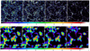 |
Fig. 1. Density fields of simulation L256 without additional smoothing and with a smoothing length 8 h−1 Mpc are shown in the upper and bottom panels, respectively. The panels from left to right show fields for epochs z = 30, z = 10, z = 3, and z = 0, presented in slices of size 200 × 200 × 0.5 h−1 Mpc. Only over-density regions are shown with colour scales from left to right 1−1.4, 1−2, 1−4, and 1−8 in the upper panels and 1−1.08, 1−1.25, 1−1.8, and 1−5 in the lower panels. |
In the upper panels we show the evolution of small-scale elements of the cosmic web, galaxies and clusters of galaxies. During the evolution, they merge to form a sharp filamentary structure at the present epoch. This evolution is predicted by the theoretical models of Arnold et al. (1982), Bond et al. (1996), and others. In the lower panels, the evolution of supercluster-scale elements of the cosmic web is shown. Superclusters alter their pattern very little during the evolution, only the amplitude of density fluctuations increases.
The density field method was used to select and study various components of the cosmic web: clusters, filaments, superclusters, voids, etc. These elements are individual objects, located in different areas of the universe. Their volumes do not overlap, but in sum, these components fill the whole universe. There exists a large number of various methods for investigating the structure and evolution of these components of the universe. For recent studies, see proceedings of the Zeldovich conference by van de Weygaert et al. (2016).
Because of its integrated nature, the PDF does not allow selecting individual components of the cosmic web. The PDF of the density field and its moments are integrated quantities that characterise properties of the whole web. Objects of various compactness of the cosmic web can be highlighted using a smoothing of the density field with different scales. Examples of various smoothing scales were shown in Fig. 1. Smoothing with small lengths, Rt ≤ 1 h−1 Mpc, highlights the whole cosmic web in the volume under study on scales of haloes and subhaloes of ordinary galaxies and poor clusters. Medium smoothing lengths, Rt = 2, 4 h−1 Mpc, are suited to highlighting the cosmic web on scales of rich clusters of galaxies and the central regions of superclusters. A large smoothing with Rt = 8 − 16 h−1 Mpc highlights the cosmic web on the supercluster scale.
Instead of “cosmic web at smoothing scale Rt”, we use the term “populations of the cosmic web” according to the smoothing length that is applied to calculate the density field. Populations cover the whole cosmic web, they characterise the web on the selected smoothing scale. The smoothing scale is a physical parameter that allows highlighting the cosmic web at the scale of interest. Using various smoothing lengths, we can study the hierarchy of structures in the cosmic web.
To quantitatively describe the evolution of the populations of the cosmic web, we used the skewness S and kurtosis K (S3 and S4) as functions of the age of the universe, measured by redshift z, or as functions of the rms of the density field, σ. These functions depend on the power spectrum index n and on other cosmological parameters of the model (Ωm, ΩΛ). The simulation epoch, z, and the smoothing length, Rt, are parameters. Every simulation of the evolution with fixed values of the parameters z and Rt yields a dot in the evolutionary diagrams.
We call the graphs in which lines join simulations with a given smoothing length Rt at various z the “evolutionary tracks” of cosmic web populations, and the graphs in which lines join simulations with various smoothing length Rt at a given epoch z the “evolutionary diagrams”. This follows the analogy with stellar evolution tracks and Hertzsprung-Russel diagrams. Evolutionary tracks show evolutionary trajectories of populations of the cosmic web at various characteristic scales in the S(z), K(z), S(σ), K(σ), and S3, 4(z), S3, 4(σ) plots. Evolutionary diagrams show where characteristic populations of the cosmic web are situated in these diagrams at various epochs. Evolutionary tracks and diagrams are based on identical data, only the data points are joined differently by the lines.
Evolutionary tracks and diagrams display the evolution of the asymmetry of the cosmic web in a simple way. Each plot shows at a glance the growth of the asymmetry of the whole web on different scales.
3. Analysis
In this section we describe the evolution of the cosmic web in the ΛCDM model through its PDF moments. Next, we investigate the evolution of the skewness S and the kurtosis K. Thereafter, we analyse skewness and kurtosis as functions of rms of the density field σ and their change with cosmic epoch and smoothing length. These relations are described first for mathematical and then for cosmological moments. In the first subsections, we mostly use results obtained with GADGET simulations. In the last subsection, we present results obtained with both simulation series.
3.1. Evolution of the PDF of ΛCDM simulations
Figure 2 shows the evolution of the PDF using the cubic-cell smoothing window. We used as argument the reduced density ν = δ/σ. This presentation is useful to show how the density distributions of our simulations can be represented by a Gaussian distribution. We show the density fields of simulation L1024 using three smoothing lengths Rt = 4, 8, and 16 h−1 Mpc from left to right. The PDFs of simulations L512 and L256 are very similar. The colour-coding indicates the evolutionary epoch, z = 30, 10, 5, 3, 1, and 0.
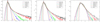 |
Fig. 2. Density distribution functions P(δ) as functions of the DM density contrast δ normalised to the rms of density fluctuations ν = δ/σ for simulation L1024 smoothed with the cubic-cell method. Panels from left to right: smoothing lengths Rt = 4, 8, 16 h−1 Mpc, indicated as the first index in the simulation name and the redshift coded in the second index. Dashed curves show the Gaussian distribution. |
The PDFs of our density fields, obtained with cubic-cell smoothing, are very similar to the PDFs found in previous studies for epochs z ≤ 3; for an example, see Shin et al. (2017). All P(ν) curves in low-density regions, ν ≤ 0, lie below the Gaussian curve and are in high-density regions, ν ≥ 5, above the Gaussian PDF. This behaviour is expected for PDFs with positive skewness.
Two conclusions are evident from this figure: (i) PDFs are asymmetric in the sense that high-density regions extend much farther than low-density regions; and (ii) smoothing has a dominant role in determining the width of the PDF distribution. Both the asymmetry and the importance of smoothing role of PDFs have been known for a long time; for early work, see Bernardeau (1994), Kofman et al. (1994), and Bernardeau & Kofman (1995). The dependence of PDFs on smoothing length was recently studied by Shin et al. (2017) and Klypin et al. (2018). In our study, we see the growth of the asymmetry in a very broad redshift interval, from z = 30 to z = 0.
3.2. Evolution of the variance, skewness and kurtosis with cosmic epoch z
Figure 3 presents the dependence of the PDF moments of simulation L512 on the cosmic epoch z. In the left panels the dependence is shown for the skewness S(z) and the kurtosis K(z), and in the right panels for the respective cosmological functions S3(z) and S4(z). Coloured lines joining symbols are the evolutionary tracks of populations of various richness, identified by the smoothing lengths. The horizontal axes are inverted to show the evolution from left to right as in the following figures. If we join points at given epochs z, we obtain evolutionary diagrams. In this representation, they are vertical lines. The error bars shown in this and the following figures were calculated using the recipes described in Appendix A.3.
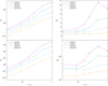 |
Fig. 3. Dependence of the PDF moments on the cosmic epoch z for simulation L512. Left top and bottom panels: dependence for the skewness S(z) and the kurtosis K(z), respectively, and right panels: their cosmological equivalents S3(z) and S4(z). The index in the simulation name is the smoothing length in h−1 Mpc. |
The evolution of the skewness S(z) and of the kurtosis K(z) are dominated by the increase in variance σ2(z) with time. The growth of the skewness S(z) is approximately proportional to the growth of σ(z), and the growth of the kurtosis K(z) is proportional to the growth of the variance σ2(z). During the evolution from z = 30 to z = 0, the amplitude of the skewness S(z) increases about 30 times and that of the kurtosis K(z) increases by a factor of one thousand. The other important aspect is the dependence of the amplitudes of the skewness and kurtosis curves on the smoothing length Rt. At the present epoch, the value of the skewness S(0) is for the smoothing length Rt = 2 h−1 Mpc, ten times higher than for smoothing length Rt = 16 h−1 Mpc; the difference in kurtosis K(0) is two orders of magnitudes.
The rate of the evolution of moments can be characterised by the logarithmic gradient,
for the skewness S(z) and a similar relation for the kurtosis K(z). Figure 4 shows the mean logarithmic gradients for the redshift range 0 ≤ z ≤ 30 of the skewness and kurtosis, ⟨γS⟩ and ⟨γK⟩, as functions of the smoothing length, Rt. Figures 3 and 4 show that the negative gradients of the skewness, γS, and of the kurtosis, γK, change with epoch and smoothing length Rt.
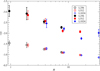 |
Fig. 4. Mean logarithmic gradients for the redshift range 0 ≤ z ≤ 30 of the skewness, ⟨γS⟩, and the kurtosis, ⟨γK⟩, as functions of the smoothing length, Rt. Open symbols show the skewness S, and filled symbols show the kurtosis K. For clarity, the symbols for simulations L256 and L1024 are slightly shifted in Rt coordinate. |
The rapid change in skewness S(z) and kurtosis K(z) with cosmic epoch z is eliminated when their cosmological equivalents, S3(z) and S4(z), are used, which we show in the right panels of Fig. 3. Here the dependence of the evolution of the skewness S3(z) and of the kurtosis S4(z) on the smoothing length Rt is very clear.
We note that the cosmic epoch z and the smoothing length Rt uniquely determine the position of the model universe in S(z), K(z), S3(z), and S4(z) functions and vice versa: any fixed value of these functions uniquely determines the z and Rt parameters of the models (for identical cosmological parameters).
3.3. Evolutionary tracks and diagrams of cosmic web populations in S(σ) and K(σ)
In Fig. 3 the evolutionary routes of populations are shown using as argument the epoch z. Another possibility to present the evolutionary routes is to use as argument the density field σ instead of z. The relations S(σ) and K(σ) were first investigated by Kofman et al. (1994). We show these relations in Fig. 5 for simulation L512. The left panels show the skewness S(σ) and right panels the kurtosis K(σ). In the top panels, the evolutionary tracks are presented, and curves join various populations. In the bottom panels, the evolution diagrams are shown. Here, simulations of identical age are connected by coloured curves that link the four smoothing lengths 2, 4, 8, and 16 h−1 Mpc. Error bars are also marked. Other simulations yield similar pictures. Because of the differences in resolution, data for simulation L256 are slightly shifted toward higher σ and data for the L1024 simulation toward lower σ.
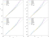 |
Fig. 5. Top panels: evolutionary tracks. Bottom panels: evolutionary diagrams. Left panels: skewness S. Right panels: kurtosis K. In the evolutionary tracks, the symbols along the tracks from left to right are for redshifts z = 30, 10, 5, 3, 1, and 0. In the evolutionary diagrams, the symbols from top to bottom correspond to smoothing lengths 2, 4, 8, and 16 h−1 Mpc. The solid bold black curves show the skewness S(σ) and kurtosis K(σ) according to the log-normal distribution. The dashed curves show S = 3σ and K = 16σ2. |
The populations have different values of σ. In this representation, populations of the same age but different smoothing length are therefore shifted along the σ coordinate. It is remarkable that the shift in σ causes evolutionary tracks of different smoothing lengths to almost coincide, as shown in Fig. 5. This coincidence led Kofman et al. (1994) to the conclusion that a range of σ values could be obtained either by analysing the system at different epochs z or by using different smoothing lengths Rt. As we show below, the dependence of the skewness and kurtosis on z and Rt is different.
Figure 5 shows that the overall mean evolution of the skewness S(σ) and the kurtosis K(σ) is proportional to the first and second power of σ, in accordance with the definition Eqs. (9) and (10). The figure also shows that the evolution on various scales is different. We discuss these differences in more detail in the next subsection.
Figure 5 also shows S(σ) = S3 σ and K(σ) = S4 σ2 curves for the log-normal PDF distribution. At small rms of the density field, σ ≤ 0.5, the log-normal distributions of S(σ) and K(σ) are power laws with indices 1 and 2, respectively. For larger σ, the log-normal law bends upwards to imitate the dependence of S(σ) and K(σ) on the smoothing length.
3.4. Evolutionary tracks and diagrams of cosmic web populations in S3(σ) and S4(σ)
The evolution of the skewness S(σ) and kurtosis K(σ) is dominated by changes in the rms of the density field σ. A much more compact presentation of the evolution is possible when we use cosmological parameters according to the definitions Eqs. (9) and (10), S3(σ) = S(σ)/σ and S4(σ) = K(σ)/σ2.
This version of evolutionary tracks and diagrams is presented in Fig. 6. It is based on data for simulation L512. As explained in Sect. 2, in evolutionary tracks (top panels), the coloured curves join the S3(σ) and S4(σ) values for various smoothing lengths Rt. Moving along the tracks from left to right, the asymmetry and flatness parameters of the cosmic web at given smoothing lengths change with redshift. The populations selected with Rt ≤ 2 h−1 Mpc and shown by cyan curves have maxima S3 ≈ 11 at z ≈ 2, and decrease in S3 for later epochs, z ≤ 2. The populations selected with a smoothing length Rt = 4 h−1 Mpc and shown by green curves reach amplitudes S3 ≈ 7 at the present epoch. The populations selected with a smoothing length Rt = 8 h−1 Mpc and shown by light blue curves have a moderate increase in S3(σ). A similar increase was found by Shin et al. (2017) for epochs z ≤ 4, see their Fig. 4. The authors used top-hat smoothing with Rt = 10 h−1 Mpc. The populations selected with a smoothing length Rt = 16 h−1 Mpc have approximately constant S3(σ) levels during the evolution; see the orange curve in the top left panel of Fig. 6.
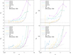 |
Fig. 6. Top panels: evolutionary tracks. Bottom panels: evolutionary diagrams. Left panels: skewness S3. Right panels: kurtosis S4. In the evolutionary tracks, the symbols along the tracks from the left are for redshifts z = 30, 10, 5, 3, 1, and 0. In the evolutionary diagrams, the symbols from top to bottom correspond to smoothing lengths 2, 4, 8, and 16 h−1 Mpc. The solid black curves show the cosmological skewness S3 and kurtosis S4 according to the log-normal distribution. The dotted curves show the predictions of the perturbation theory Eq. (11). |
The evolutionary tracks of the kurtosis S4(σ) are shown in the top right panel of Fig. 6. The general shape of tracks is similar, only the growth of S4(σ) for small smoothing lengths and late epochs is much stronger. The S4(σ) evolutionary tracks are more affected by errors, both sampling errors, shown as error bars in Fig. 6, and possible systematic errors, discussed in Appendix B. When we take these possible errors into account, the increase in S3(σ) and S4(σ) with decreasing smoothing length is a general property of the evolution.
The bottom panels in Fig. 6 show evolutionary diagrams of the populations for simulation L512: curves joining symbols connect simulations of identical redshift z. As in Fig. 5, for each epoch, the symbols from the top down correspond to smoothing lengths Rt = 2, 4, 8, and 16 h−1 Mpc. The evolutionary diagrams for different ages are well separated from each other and are located at approximately similar mutual distances along the σ-axis. This conclusion is valid for both S3(σ) and S4(σ).
We show in all panels the S3(σ) and S4(σ) functions as predicted by the perturbation theory, Eq. (11), for the same set of smoothing lengths and redshifts. The comparison shows that for redshift z = 30 and large smoothing lengths, the PT is in fairly good agreement with the results of numerical simulations. For a lower redshift and smaller smoothing lengths, the PT is not able to reproduce the S3(σ) and S4(σ) functions found in simulations. Differences increase with the decrease in smoothing length.
Figure 7 shows the results of the GLAM simulations for the skewness S3(σ) and kurtosis S4(σ). Here we combined data from six GLAM simulations, all with many realisations, therefore the shot noise is much smaller. Data for different boxes agree quite well within 2 − 3%. In the top panels, the coloured curves join simulations with identical smoothing lengths, and in the bottom panels, they join simulations of identical redshift, that is, we have evolutionary tracks and diagrams, respectively.
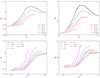 |
Fig. 7. Top panels: evolutionary tracks. Bottom panels: evolutionary diagrams. Left panels: skewness S3. Right panels: kurtosis S4. The shaded areas correspond to the 1σ statistical uncertainties. |
The evolutionary tracks of populations are shown in great detail, especially for populations with small smoothing lengths. At the lowest smoothing length, the peaks of S3(σ) and S4(σ) are at redshift z = 5, followed by a slow decrease at lower redshifts. The evolution is shown for five smoothing lengths from Rt = 0.5 h−1 Mpc to Rt = 10.6 h−1 Mpc. Moving along tracks from left to right, S3(σ) and S4(σ) change during the evolution from z = 10 to z = 0. In this figure, the points for various redshifts are not marked.
The evolutionary diagrams were calculated for seven redshifts, starting from z = 20. The lower tips of the curves in most cases correspond to the smoothing length Rt = 10.6 h−1 Mpc, and the upper tips show the lowest smoothing length Rt = 0.5 h−1 Mpc. Figure 7 shows that the evolutionary diagrams have a more complex structure than expected from simulations with lower resolution. For smaller smoothing lengths, Rt ≤ 2 h−1 Mpc, and recent epochs, z ≤ 1, the diagrams reach constant levels. All curves for changing z and Rt yield monotonic ladders without crossing each other. The GLAM simulations confirmed all basic findings from the GADGET simulations with high confidence, and they suggested some important details that were not observed in simulations with low-mass resolution.
The comparison of Figs. 6 and 7 shows that the evolutionary tracks found with the GADGET and GLAM simulations are qualitatively very similar. Both start at high redshifts (small σ) at levels S3 ≈ 3.5 and S4 ≈ 25, and have maxima of the S3(σ) and S4(σ) curves for different smoothing lengths at similar σ and redshift z values. In Fig. 8 we show the maxima of the skewness S3 and kurtosis S4 evolutionary tracks as functions of the smoothing length Rt. The redshifts of the maxima depend on the smoothing length Rt. For a small smoothing length Rt = 0.5 h−1 Mpc, the maxima are located at redshift z ≈ 5, and for Rt = 1 h−1 Mpc, they lie at z ≈ 1. For greater smoothing lengths Rt ≥ 2.6, the maximum is not reached, see the upper panels of Fig. 7. In these cases, we accepted as maximum the S3 and S4 value at redshift z = 0. We ignore in Fig. 8 the redshift dependence of the maxima.
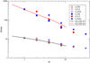 |
Fig. 8. Maxima of the skewness S3 and kurtosis S4 evolutionary tracks as functions of the smoothing length Rt. Open symbols show the skewness S3 and filled symbols show the kurtosis S4 for GADGET simulations of various cube lengths L0. The black and red curves show the maxima of the S3 and S4 curves of the GLAM simulations. |
Figure 8 shows that an almost linear relationship exists between maxima and smoothing length in the log−log presentation. There is a scatter of the maxima that is found with GADGET simulations for different cube lengths, which is larger than expected from the sampling errors. However, the overall trend with Rt is similar for all simulations, thus the scatter is likely caused by difficulties of determination of moments, as discussed in Appendix B. The curves S3(Rt) and S4(Rt) for the GLAM simulations are located within the range expected from the GADGET simulations. Thus we see that GADGET and GLAM simulations yield very similar results for PDF moments in quantitative terms as well.
The presence of the maxima in the evolutionary tracks shows the change in the rate of the growth of the asymmetry of the cosmic web, measured by the logarithmic gradients γS(z) and γK(z), see Eq. (15). At the maxima of S3(z) and S4(z), the gradients γS(z) and γK(z) change, that is, the rate of the growth of the asymmetry slows. On smaller scales, highlighted by small Rt, the change occurs at higher redshifts.
4. Discussion
In this section we discuss the growth of the density fluctuations and the evolution of the particle densities using theoretical models. We then compare our results with earlier results. Finally, we discuss the cosmological interpretation of our data.
4.1. Comparison with theoretical models
An important conclusion from our data is that the dependences of the PDF moments on the evolutionary epoch z and on the smoothing length Rt are very different. Figures 6 and 7 clearly demonstrate that the rms of the density fluctuations σ does not determine the moments of the PDF in a unique way. At a fixed redshift, that is, in the evolutionary diagrams, the S3 and S4 curves increase with σ at small σ ≲ 1, then they flatten out and stay constant at σ ≳ 2. The behaviour is different for fixed Rt, that is, in evolutionary tracks. At small σ, the curves turn upwards, but then they reach a maximum and start to decline. Regardless of the selection (constant z or constant Rt), the curves show a complex behaviour. For example, the position and amplitude of the maximum of S3 change with Rt if Rt is fixed. For fixed z, the amplitude and the redshift z of the plateau depend on the redshift.
The results presented in Figs. 6 and 7 show interesting and somewhat counter-intuitive features: at the same rms of the fluctuations σ, the deviations from the Gaussian distribution are stronger at high redshifts z. It might naively be expected that as the fluctuations grow, the PDF becomes more non-Gaussian. However, at first sight, the reverse occurs. For example, in the top panels of Fig. 7 (evolutionary tracks), the factors S3 and S4 decrease with decreasing redshift at fixed σ.
In order highlight this effect, in Fig. 9 we plot the PDFs selected at two different redshifts that have the same σ = 0.8. It is clear that at z = 5, the PDF is much broader and more evolved than at z = 0. The key issue here is that the filtering scale Rt is dramatically different for z = 5 and z = 0. In order to have the same σ at high redshift, the filtering scale needs to be decreased. In our case, this amounts to changing Rt from 10 h−1 Mpc at z = 0 to 0.5 h−1 Mpc at z = 5. Or in different terms: at redshift z = 5, small-scale structures of the cosmic web, highlighted by smoothing with Rt = 0.5 h−1 Mpc, are more asymmetric than supercluster-scale structures at the present epoch.
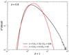 |
Fig. 9. Comparison of the PDFs with the same rms fluctuations σ = 0.8, but estimated at different redshifts z = 0 and z = 5. The PDFs are scaled with δ3 to reduce the dynamical range. The filtering scales are Rt = 10 h−1 Mpc at z = 0 and Rt = 0.5 h−1 Mpc at z = 5. |
This effect becomes quite obvious when we understand why it occurs. However, it presents a problem for non-linear models of the PDF, such as the lognormal distribution where the rms of the density perturbation σ is the only factor that defines the PDF. These models cannot possibly account for the evolution of the PDF with redshift.
The predictions of the PT calculated with Eq. (11) and presented in Fig. 6 suggest the dependence of S3 and S4 on the effective slope of the power spectrum of the perturbations at radius R as γ = −(neff + 3). This only affects the height of values S3 and S4, see the ladder of dotted lines in the top panels of Fig. 6 for different Rt and the lines in bottom panels of Fig. 6 for different z. No strong increase in S3 and S4 for later evolutionary epochs, z ≤ 10, and smaller smoothing scales, Rt ≤ 4, is predicted.
In Fig. 10 we compare the evolution of S3(σ) of the GLAM simulations with results of the PT, the lognormal distribution, and an analytical fit. The new analytical approximation is described in the next subsection. The fit uses as input σ and redshift z and gives S3 and S4 using an approximation of four free parameters. It works well and can be useful for predictions. The log-normal and PT results are not very accurate. The log-normal distribution does not have any dependence on redshift because by design, it is a function of σ only. It fails on all scales, small and large σ, and even at high redshifts. The PT approximation predicts some evolution with redshift, but the magnitude of the effect is just too small.
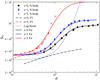 |
Fig. 10. Comparison of S3(σ, z) for redshifts z = 0, 1, and 5 found in N-body simulations with the predictions of the PT, Eq. (11), and the log-normal distribution, Eq. (14). |
4.2. Analytical approximations for the evolution of skewness and kurtosis
We fitted the results of the evolution of S3(σ) and S4(σ) using a four-parameter functional form. If S is either S3 or S4, then the approximation can be written as
where Smin is the minimum value of S, and parameters C1 and C2 describe the shape of the function S(σ). Specifically, the ratio C1/C2 gives the magnitude of the total increase in S,

Another shape parameter is S1, which is the value of S at σ = 1. Using parameters Smin, S1, and Smax, we can find C1 and C2,
The evolution of S is described by a power-law dependence of S1 and Smax on redshift z,

where α is a free parameter describing the evolution with time. Here S10 and Smax, 0 are shape parameters estimated at z = 0.
This approximation has four free parameters: three shape parameters Smin, S10, and Smax, 0, and parameter α, which describes the evolution. Based on these parameters, C1 and C2 can be determined using Eq. (18). Now we can use Eq. (16) to estimate parameters S3 and S4. For the cosmology used for the GLAM simulations and for a reduced skewness S3, the parameters are S3, min = 3.5, S3, 10 = 4.9, and S3max, 0 = 9.4. Parameter α depends on redshift. We find that for z ≲ 1.5, the parameter is α = 0.25. For higher redshifts, the evolution is slightly faster: α = 0.43. These approximations give a 5% accuracy for S3. This fit was tested and can only be used for z ≲ 20 and for σ > 0.05.
4.3. Comparison with earlier results
Only a few studies exist of the moments of the PDF on the basis of numerical simulations of the evolution of the density field. We summarise the results from different simulations in Table 3. Authors have used different cosmological parameters in simulations and various redshift intervals and smoothing lengths. A direct comparison of the skewness and kurtosis parameters is not easy.
Estimates of the skewness and kurtosis parameters.
Only a few authors provided results of the evolution of the S3 and S4 parameters in cosmological N-body simulations, and none of them provided data for the dependence on the amplitude of the density fluctuations σ. Shin et al. (2017) showed results for the evolution of the S3 parameter for a top-hat filter with radius RTH = 10 h−1 Mpc. Our results are very similar to theirs for the same effective volume, although there are differences on a level of a few percent. Mao et al. (2014) showed results for z = 0 and RTH = 10 h−1 Mpc, which also agree with our results within ∼10% errors.
There is a reason for the lack of interest in the evolution of the PDF with time: it is expected that the PDF depends on time only through the amplitude of perturbations σ. In other words, it is expected that P(ρ) = P(ρ; σ(z, R)). Perturbation theory (e.g. Juszkiewicz et al. 1993; Bernardeau 1994) predicts some explicit dependence on z, as can been seen in Eq. (11). However, the dependence on redshift is very weak. At the same time, non-linear approximations based on top-hat collapse or spherical infall models (e.g. Betancort-Rijo & López-Corredoira 2002; Lam & Sheth 2008) only depend on σ and not explicitly on the redshift.
As our results clearly show, an explicit evolution with the redshift is clearly present and quite strong. This suggests that some presumptions, on which the PT is based, need revision.
4.4. Cosmological interpretation
4.4.1. Contrasting the evolution of the cosmic web on small and large scales
One of the findings of our study is the contrast between the evolution of the cosmic web on small and large scales, as defined by the smoothing length Rt. The cosmic web populations defined by a large smoothing length Rt ≥ 10 h−1 Mpc, at all cosmic epochs have S3 ≤ 4 and S4 ≤ 35. The cosmic web populations defined by a small smoothing length Rt ≤ 2 h−1 Mpc, at late evolutionary epochs z ≤ 5 have maxima of moments S3 ≥ 10 and S4 ≥ 150.
To understand the reason for this difference, we recall that the cosmological moments S3 and S4 are actually amplitude parameters of the mathematical skewness S = S3 × σ and kurtosis K = S4 × σ2, as defined by Eqs. (9) and (10). The data presented in Figs. 6 and 7 can be expressed as functions of redshift of the mathematical skewness S(z) and kurtosis K(z), as done in Fig. 3. The evolution of large-scale populations of the cosmic web proceeds with an almost constant rate that is measured by the mean logarithmic gradients, ⟨γS⟩≈ − 1 and ⟨γK⟩≈ − 2, shown in Fig. 4. The speed of the evolution of the small-scale elements, characterised by a small smoothing length Rt, is much faster: for Rt = 1 h−1 Mpc ⟨γS⟩≈ − 1.5 and ⟨γK⟩≈ − 3, see Fig. 4.
The increase in the (negative) gradient in the interval z ≤ 10 is due to the non-linear growth of density perturbations, which is important for small-scale perturbations. The relative decrease in the gradient for z ≤ 1 is due to the effect of the Λ term.
4.4.2. Similarity of the evolution of the skewness and kurtosis
We note one important property of the PDFs of the cosmic web: the shapes of the S3(σ) and S4(σ) curves are qualitatively very similar, as shown in Fig. 6 and especially in Fig. 7. This property is due to the character of the density field of the cosmic web. It is highly asymmetric, all details of the structure are in over-density regions, and the under-density region is almost structure-less. We conclude that the two PDF moments, the skewness S(σ) and the kurtosis K(σ) (and their amplitudes S3(σ) and S4(σ)), essentially measure the asymmetry of the density field. However, large quantitative differences exist: at the maxima, S4(σ) are larger than S3(σ) by a factor of 10 to 50, see Fig. 8.
4.4.3. Independent evidence for the asymmetry of the density field
The asymmetry of the evolution of the density perturbations is reflected not only in the PDF of the density field as measured by the skewness parameter S. It is also seen in the distribution of particle densities, as shown by Pandey et al. (2013). Asymmetry is also observed in the distribution of the number of superclusters as a function of the reduced density, ν = δ/σ, see Fig. 1 by Einasto et al. (2019) and Fig. 2 by Einasto et al. (2021).
According to our assumptions, the evolution of the universe started from a Gaussian random field that was symmetrical around the mean density, that is, positive and negative deviations from the mean density are equally probable. The question thus is at which time the density field became asymmetric.
To explore the problem, we investiage the evolution of the structure shown in Fig. 1. For example, supercluster-type elements are visible almost in the same form already at the earliest epoch, z = 30, and they change little at the late stage of the evolution. Cluster-type elements are also seen in the early universe, but they change much during the evolution. These differences illustrate the numerical data of the evolution on various scales, shown in Fig. 6. For our study, the presence of both small- and large-scale elements of the cosmic web already at early stages of the evolution is important.
Another manifestation of the early evolution of the cosmic web is the almost constant number of superclusters during the evolution, see Fig. 2 in Einasto et al. (2019) and Fig. 6 in Einasto et al. (2021). This suggests that supercluster embryos were created in the very early universe, much earlier than is seen in the density field of the cosmic web at redshift z = 30. The difference between positive and negative density perturbations lies in the fact that positive perturbations form distinct structures, embryos of galaxies, clusters, and superclusters, already at the very early stages of the evolution, whereas negative perturbations of similar strength form voids and act as structure-less repellers. The asymmetry parameter, the mathematical skewness S, measures this difference in positive and negative perturbations.
4.4.4. PDF moments in the early universe
The behaviour of the skewness and kurtosis at very early epochs is of interest. Figures 6 and 7 show that all S3(σ) and S4(σ) curves approach with increasing z limiting values, depending on the scale of systems, as determined by smoothing length. In this way, our analysis confirmed earlier results by Bernardeau & Kofman (1995), Hellwing et al. (2010, 2017), and Mao et al. (2014).
We cannot answer the question how PDF moments S(σ), K(σ), S3(σ) and S4(σ) behave at very small σ at the moment. The cosmic density field can have small rms of density fluctuations σ in a young universe at high redshift z, or using a very large smoothing length Rt. Our data suggest that in a young universe, the PDF moments converge with increasing z to limits S(σ) = S3 σ, and K(σ) = S4 σ2 with S3 ≈ 3 and S4 ≈ 15. The limited range of the smoothing lengths Rt used in our simulations gives no hint to S3(σ) and S4(σ) for very large smoothing. Future studies are needed to solve this question.
4.4.5. Early evolution of the universe
The early evolution of the density field was calculated in simulations using the Zeldovich approximation, thereafter, actual numerical simulations follow. Available data suggest that embryos of galaxies and superclusters were created by high peaks of the initial field. The initial velocity field around the peaks is almost laminar. The highest density peaks of the density field started to attract surrounding matter more strongly than around peaks of lower density. In this way, centres of future galaxies, clusters, and superclusters formed. The almost identical pattern of the cosmic web on the supercluster scale at epochs with z ≥ 3 suggests that the same pattern existed at earlier epochs, even soon after the creation of density fluctuations. The development of the density field in the early phase is well described by the Zeldovich (1970) approximation and its extension, the adhesion model by Kofman & Shandarin (1988). As shown by Kofman et al. (1990, 1992), the adhesion approximation for the present epoch yields structures that are very similar to the structures calculated with N-body numerical simulations of the evolution of the cosmic web with the same initial fluctuations. Thus the combination of theoretical models and numerical simulations suggests that the asymmetry of the PDF started to form soon after the creation of fluctuations in the early period of the evolution of the universe.
5. Conclusions
We studied the evolution of the DM density field with the goal of determining evolutionary changes in one-point PDF and its moments. We used a large set of input parameters of N-body simulations, the box size, L0, the smoothing length, Rt, and the simulation epoch, z, to follow the evolution of ΛCDM models. We performed numerical simulations of ΛCDM models for two sets of simulations, one with Ngrid = 512, and the other with Ngrid = 2000, 5000. In these sets we used different cosmological parameters, simulation algorithms, and simulation box sizes. We calculated density fields for several series of smoothing lengths using various smoothing rules.
For all simulation sets, we calculated one-point PDFs and their moments, the standard deviation σ, the skewness S, and the kurtosis K. The mathematical skewness S characterises the degree of asymmetry of the distribution, while the kurtosis K measures the presence of heavy tails and peaks in the distribution. Simple relations exist between mathematical and cosmological parameters: the skewness S = S3 × σ, and the kurtosis K = S4 × σ2, where S3 and S4 are the cosmological skewness and kurtosis, that is, the cosmological skewness and kurtosis, S3 and S4, play the role of amplitude parameters of the mathematical S and K.
Our study extends previous studies by analysing both mathematical and cosmological skewness and kurtosis, using a wide range of evolutionary epochs from z = 30 on, and a wide range of smoothing lengths from Rt = 0.4 to Rt = 32 h−1 Mpc. We defined populations of the cosmic web by the smoothing length Rt, which is used to calculate PDF moments.
The basic conclusions of our study are listed below.
-
The moments S and K, calculated for density fields at different cosmic epochs and smoothed with various scales, characterise the evolution of different structures of the web. The moments calculated with small-scale smoothing (Rt ≈ 1 − 4 h−1 Mpc) characterise the evolution of the web on a cluster-type scale. The moments found with large smoothing (Rt ≳ 5 − 15 h−1 Mpc) describe the evolution of the web on a supercluster scale.
-
During the evolution, the cosmological skewness S3 = S/σ and cosmological kurtosis S4 = K/σ2 present a complex behaviour: at a fixed redshift, the curves of S3(σ) and S4(σ) steeply increase with σ at σ ≲ 1 and then flatten out and become constant at σ ≳ 2. If we fix the smoothing scale Rt, then after reaching the maximum at σ ≈ 2, the curves at large σ start to gradually decline. We provided accurate fits for the evolution of S3, 4(σ, z). Skewness and kurtosis approach constant levels at early epochs: depending on the smoothing length, S3(σ)≈3 and S4(σ)≈15, respectively.
-
Direct and indirect data suggest that seeds of elements of the cosmic web were created at early epoch at inflation and started to grow thereafter. This explains the continuous growth of the asymmetry of the density distribution, expressed by the skewness S and kurtosis K functions.
We find that the evolution of S3 and S4 cannot be described by current theoretical approximations. The often-used lognormal distribution function for the PDF fails to explain even qualitatively the shape and evolution of S3 and S4. We still have no definite answer to the question how the PDF moments behave at very small σ. The cosmic density field has a small rms of the density fluctuations in a young universe and in the universe at the present age, applying a very large smoothing length of the density field. The limited range of the smoothing lengths used in our simulations gives no hint to S3 and S4 for very large smoothing.
Acknowledgments
We thank Ivan Suhhonenko for performing GADGET simulations, used in this study, Enn Saar for discussion, and anonymous referee for very stimulating suggestions, which helped in improve the paper. This work was supported by institutional research funding IUT40-2 of the Estonian Ministry of Education and Research, by the Estonian Research Council grant PRG803, and by Mobilitas Plus grant MOBTT5. We acknowledge the support by the Centre of Excellence “Dark side of the Universe” (TK133) financed by the European Union through the European Regional Development Fund.
References
- Arnold, V. I., Shandarin, S. F., & Zeldovich, I. B. 1982, Geophys. Astrophys. Fluid Dyn., 20, 111 [NASA ADS] [CrossRef] [Google Scholar]
- Bernardeau, F. 1994, ApJ, 433, 1 [NASA ADS] [CrossRef] [Google Scholar]
- Bernardeau, F., & Kofman, L. 1995, ApJ, 443, 479 [NASA ADS] [CrossRef] [Google Scholar]
- Bernardeau, F., Colombi, S., Gaztañaga, E., & Scoccimarro, R. 2002, Phys. Rep., 367, 1 [NASA ADS] [CrossRef] [EDP Sciences] [MathSciNet] [Google Scholar]
- Bertschinger, E. 1995, ArXiv e-prints [arXiv:astro-ph/9506070] [Google Scholar]
- Betancort-Rijo, J., & López-Corredoira, M. 2002, ApJ, 566, 623 [NASA ADS] [CrossRef] [Google Scholar]
- Bond, J. R., & Myers, S. T. 1996, ApJS, 103, 1 [NASA ADS] [CrossRef] [Google Scholar]
- Bond, J. R., Kofman, L., & Pogosyan, D. 1996, Nature, 380, 603 [NASA ADS] [CrossRef] [Google Scholar]
- Bouchet, F. R., & Hernquist, L. 1992, ApJ, 400, 25 [CrossRef] [Google Scholar]
- Bouchet, F. R., Juszkiewicz, R., Colombi, S., & Pellat, R. 1992, ApJ, 394, L5 [NASA ADS] [CrossRef] [Google Scholar]
- Cadiou, C., Pichon, C., Codis, S., et al. 2020, MNRAS, 496, 4787 [Google Scholar]
- Catelan, P., & Moscardini, L. 1994, ApJ, 426, 14 [CrossRef] [Google Scholar]
- Coles, P., & Jones, B. 1991, MNRAS, 248, 1 [NASA ADS] [CrossRef] [Google Scholar]
- Davison, A. C., & Hinkley, D. V. 1997, Bootstrap Methods and Their Application (Cambridge, UK: Cambridge University Press) [CrossRef] [Google Scholar]
- de Lapparent, V., Geller, M. J., & Huchra, J. P. 1986, ApJ, 302, L1 [Google Scholar]
- Efron, B. 1982, The Jackknife, the Bootstrap and Other Resampling Plans (Stanford, CA: Stanford University) [Google Scholar]
- Einasto, J., Suhhonenko, I., Liivamägi, L. J., & Einasto, M. 2019, A&A, 623, A97 [NASA ADS] [CrossRef] [EDP Sciences] [Google Scholar]
- Einasto, J., Hütsi, G., Suhhonenko, I., Liivamägi, L. J., & Einasto, M. 2021, A&A, 647, A17 [CrossRef] [EDP Sciences] [Google Scholar]
- Fry, J. N., & Gaztanaga, E. 1993, ApJ, 413, 447 [NASA ADS] [CrossRef] [Google Scholar]
- Gaztanaga, E., & Bernardeau, F. 1998, A&A, 331, 829 [Google Scholar]
- Gaztañaga, E., Fosalba, P., & Elizalde, E. 2000, ApJ, 539, 522 [NASA ADS] [CrossRef] [Google Scholar]
- Gregory, S. A., & Thompson, L. A. 1978, ApJ, 222, 784 [NASA ADS] [CrossRef] [Google Scholar]
- Hellwing, W. A. 2010, Ann. Phys., 19, 351 [CrossRef] [Google Scholar]
- Hellwing, W. A., & Juszkiewicz, R. 2009, Phys. Rev. D, 80, 083522 [CrossRef] [Google Scholar]
- Hellwing, W. A., Juszkiewicz, R., & van de Weygaert, R. 2010, Phys. Rev. D, 82, 103536 [NASA ADS] [CrossRef] [Google Scholar]
- Hellwing, W. A., Koyama, K., Bose, B., & Zhao, G.-B. 2017, Phys. Rev. D, 96, 023515 [CrossRef] [Google Scholar]
- Jing, Y. P. 2005, ApJ, 620, 559 [NASA ADS] [CrossRef] [Google Scholar]
- Jõeveer, M., & Einasto, J. 1978, in Large Scale Structures in the Universe, eds. M. S. Longair, & J. Einasto, IAU Symp., 79, 241 [Google Scholar]
- Juszkiewicz, R., Bouchet, F. R., & Colombi, S. 1993, ApJ, 412, L9 [NASA ADS] [CrossRef] [Google Scholar]
- Juszkiewicz, R., Weinberg, D. H., Amsterdamski, P., Chodorowski, M., & Bouchet, F. 1995, ApJ, 442, 39 [NASA ADS] [CrossRef] [Google Scholar]
- Kayo, I., Taruya, A., & Suto, Y. 2001, ApJ, 561, 22 [Google Scholar]
- Klypin, A., & Prada, F. 2018, MNRAS, 478, 4602 [CrossRef] [Google Scholar]
- Klypin, A., Prada, F., Betancort-Rijo, J., & Albareti, F. D. 2018, MNRAS, 481, 4588 [CrossRef] [Google Scholar]
- Kofman, L. A., & Shandarin, S. F. 1988, Nature, 334, 129 [NASA ADS] [CrossRef] [Google Scholar]
- Kofman, L., Pogosian, D., & Shandarin, S. 1990, MNRAS, 242, 200 [NASA ADS] [CrossRef] [Google Scholar]
- Kofman, L., Pogosyan, D., Shandarin, S. F., & Melott, A. L. 1992, ApJ, 393, 437 [NASA ADS] [CrossRef] [Google Scholar]
- Kofman, L., Bertschinger, E., Gelb, J. M., Nusser, A., & Dekel, A. 1994, ApJ, 420, 44 [NASA ADS] [CrossRef] [Google Scholar]
- Lahav, O., Itoh, M., Inagaki, S., & Suto, Y. 1993, ApJ, 402, 387 [NASA ADS] [CrossRef] [Google Scholar]
- Lam, T. Y., & Sheth, R. K. 2008, MNRAS, 386, 407 [CrossRef] [Google Scholar]
- Lewis, A., Challinor, A., & Lasenby, A. 2000, ApJ, 538, 473 [Google Scholar]
- Liivamägi, L. J., Tempel, E., & Saar, E. 2012, A&A, 539, A80 [NASA ADS] [CrossRef] [EDP Sciences] [Google Scholar]
- Lokas, E. L., Juszkiewicz, R., Weinberg, D. H., & Bouchet, F. R. 1995, MNRAS, 274, 730 [CrossRef] [Google Scholar]
- Mao, Q., Berlind, A. A., McBride, C. K., et al. 2014, MNRAS, 443, 1402 [NASA ADS] [CrossRef] [Google Scholar]
- Marinoni, C., Le Fèvre, O., Meneux, B., et al. 2005, A&A, 442, 801 [NASA ADS] [CrossRef] [EDP Sciences] [Google Scholar]
- Marinoni, C., Guzzo, L., Cappi, A., et al. 2008, ArXiv e-prints [arXiv:0811.2358] [Google Scholar]
- Pandey, B., White, S. D. M., Springel, V., & Angulo, R. E. 2013, MNRAS, 435, 2968 [CrossRef] [Google Scholar]
- Peebles, P. J. E. 1980, The Large-scale Structure of the Universe (Princeton: Princeton University Press) [Google Scholar]
- Pogosyan, D., Pichon, C., Gay, C., et al. 2009, MNRAS, 396, 635 [CrossRef] [Google Scholar]
- Press, W. H., Teukolsky, S. A., Vetterling, W. T., & Flannery, B. P. 1992, Numerical Recipes in FORTRAN. The Art of Scientific Computing (Cambridge: Cambridge University Press) [Google Scholar]
- Romeo, A. B., Agertz, O., Moore, B., & Stadel, J. 2008, ApJ, 686, 1 [NASA ADS] [CrossRef] [Google Scholar]
- Saar, E. 2009, in Data Analysis in Cosmology, eds. V. J. Martínez, E. Saar, E. Martínez-González, & M. J. Pons-Bordería (Berlin: Springer-Verlag), Lect. Notes Phys., 665, 523 [CrossRef] [Google Scholar]
- Shin, J., Kim, J., Pichon, C., Jeong, D., & Park, C. 2017, ApJ, 843, 73 [CrossRef] [Google Scholar]
- Smith, R. E., Peacock, J. A., Jenkins, A., et al. 2003, MNRAS, 341, 1311 [Google Scholar]
- Springel, V. 2005, MNRAS, 364, 1105 [Google Scholar]
- Starck, J. L., & Murtagh, F. 2006, Astronomical Image and Data Analysis (Berlin, Heidelberg: Springer-Verlag) [CrossRef] [Google Scholar]
- Szapudi, I. 2009, in Introduction to Higher Order Spatial Statistics in Cosmology, eds. V. J. Martínez, E. Saar, E. Martínez-González, & M. J. Pons-Bordería (Springer), 665, 457 [Google Scholar]
- Takahashi, R., Sato, M., Nishimichi, T., Taruya, A., & Oguri, M. 2012, ApJ, 761, 152 [Google Scholar]
- Tarenghi, M., Tifft, W. G., Chincarini, G., Rood, H. J., & Thompson, L. A. 1978, in Large Scale Structures in the Universe, eds. M. S. Longair, & J. Einasto, IAU Symp., 79, 263 [NASA ADS] [CrossRef] [Google Scholar]
- Tully, R. B., & Fisher, J. R. 1978, in Large Scale Structures in the Universe, eds. M. S. Longair, & J. Einasto, IAU Symp., 79, 214 [NASA ADS] [Google Scholar]
- Uhlemann, C., Codis, S., Hahn, O., Pichon, C., & Bernardeau, F. 2017, MNRAS, 469, 2481 [CrossRef] [Google Scholar]
- van de Weygaert, R., Shandarin, S., Saar, E., & Einasto, J. 2016, in The Zeldovich Universe: Genesis and Growth of the Cosmic Web, IAU Symp., 308 [Google Scholar]
- Zeldovich, Y. B. 1970, A&A, 5, 84 [Google Scholar]
- Zeldovich, Y. B. 1978, in Large Scale Structures in the Universe, eds. M. S. Longair, & J. Einasto, IAU Symp., 79, 409 [NASA ADS] [CrossRef] [Google Scholar]
- Zeldovich, Y. B., Einasto, J., & Shandarin, S. F. 1982, Nature, 300, 407 [NASA ADS] [CrossRef] [Google Scholar]
Appendix A: Density estimates and power spectra
A.1. Kernel density estimates
One of the ways to calculate the density field is through a kernel sum (Davison & Hinkley 1997),
where the sum is over all N data points, ri are the coordinates of data points, and K is the kernel.
Kernels K are required to be distributions that are positive everywhere and integrate to unity; in our case,
Good kernels for smoothing densities to a grid are the box splines Bk. They are local, and they are interpolating on a grid,
for any x and a small number of indices that give non-zero values for Bk(x). To create our density fields, we used the popular B3 spline function,

This function differs from zero only in the interval x ∈ ( − 2, 2), meaning that the sum in (A.3) only includes values of B3(x) at four consecutive arguments x ∈ ( − 2, 2) that differ by 1. Figure A.1 shows the shape of the function in comparison to a Gaussian. We note that in this formulation, the smoothing scale and input particle coordinates are given implicitly in units of grid cell length, and the smoothing scale is equal to one.
If we choose B3 to be our kernel function,  , then the three-dimensional kernel
  is given by a direct product of three one-dimensional kernels,

where r ≡ {x, y, z}. Although this is a direct product, it is isotropic to a very high degree (Saar 2009).
To increase the smoothing scale, we can introduce a scale parameter to the kernel function K (together with the appropriate normalisation). However, in practice, this also increases the number of particles in the kernel volume, and the computation can quickly become uneconomical. One of the benefits of using the B3 smoothing kernel is that we can employ the à trous wavelet algorithm, and having an existing density field as basis, calculate a field with twice the smoothing length by convolution with a simple discrete filter (Starck & Murtagh 2006),

Here Cj and Cj + 1 denote correspondingly the initial and smoothed density fields. Thus only the first density field needs to be calculated using particle coordinates. The convolution mask H is constructed as the following direct product:
where the coefficients h are derived from the à trous discrete wavelet transform, and its values corresponding to the B3 function are
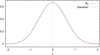 |
Fig. A.1. Shape of the box spline kernel B3. The solid curve shows the B3(x) kernel, and the dashed curve shows a Gaussian with σ = 0.6. |
A.2. Cubic-cell density estimate
Smoothing lengths of original density fields from numerical simulation output have a resolution that is equal to the size of the simulation cell, L0/Ngrid. We call this the smoothing rank zero. We used a smoothing recipe that increased the smoothing length by a factor of 2. We used this recipe successively four times, and obtained four smoothing ranks 1 to 4. For clarity, we show in the core text a smoothing length in units of h−1 Mpc.
In case of the cubic-cell smoothing, we divided the original computational box of size L0 with resolution Ngrid = 512 to boxes of smaller resolution, Ngrid = 256, 128, 64, 32, by counting densities in respective cells of the field in the previous smoothing length. This yielded smoothing lengths Rt = L0/Ngrid h−1 Mpc. Smoothing lengths for rank 1 are R1 = L0/256 h−1 Mpc, R2 = L0/128 h−1 Mpc for rank 2, and so on. The main difference between smoothing rules is that B3 spline and top-hat rules preserve the grid size, but the cubic-cell rule yields density fields with decreasing grid sizes Ngrid.
A.3. Top-hat density and error estimates
Top-hat smoothed densities for L256, L512 and L1024 simulations were calculated at the nodes of a 5123 regular cubic grid using smoothing radii for ranks 1 to 4, as explained in the previous subsection.
The errors for the moments of the density distribution were determined through jackknife resampling: a full simulation box was divided into smaller cubes, each time omitting one of the small cubes while calculating the statistical moments. The variability of the calculated moments directly gives the desired error estimates (Efron 1982). We chose to split the simulation box into 23, 43, and 83 equal-sized subcubes. The error estimates for all of these three choices did not vary significantly. In figures with error, we only use the errors for the second choice, that is, 43 = 64 subvolume case. We note that errors of all quantities (variance, K, S, S3, S4) were found separately.
The PDFs of density fields and their moments can have systematic errors. We discuss these errors in the next appendix.
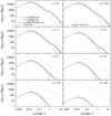 |
Fig. A.2. Comparison of simulation power spectra with the corresponding linear spectra and non-linear HALOFIT results at various epochs z. |
A.4. Evolution of the DM power spectra
Here we perform a simple consistency check for our GADGET simulations. In particular, we calculate the density power spectra for all the output redshifts and box sizes, resulting in a total of 8 × 3 = 24 spectra. The spectra were calculated using FFTs on a 10243 regular cubic grid. The simulation particles were assigned to a grid through the triangular-shaped cloud (TSC) mass-assignment scheme. The shot-noise removal, grid smoothing, and aliasing correction tailored for the TSC scheme were applied following the description given by Jing (2005).
The results of these calculations are shown in Figure A.2. Here the panels correspond to simulation snapshot redshifts displayed in the upper right corners, that is, they grow from left to right and from top to bottom. In comparison, we show the non-linear spectra according to the analytic HALOFIT approximation (Smith et al. 2003; Takahashi et al. 2012) as implemented in the cosmological Boltzmann code package CAMB1 by Lewis et al. (2000). The corresponding linear spectra (also obtained with CAMB) are plotted as well. As a reference, the dotted curves in all of the panels with z > 0 show the z = 0 non-linear spectrum.
The agreement between our simulation spectra and the well-tested analytic HALOFIT results is mostly very good. As expected, the larger boxes perform better at larger scales, while their lack of resolution at smaller scales cannot properly account for the small-scale non-linear evolution. In conjunction, except for the highest redshifts, the chosen three box sizes are reasonably good for capturing the dynamics of structure formation over more than three orders of magnitude in scale.
Appendix B: Comparison of the moments obtained with different smoothing recipes
We smoothed our GADGET simulations with three different kernels, the B3 kernel, a cubic-cell kernel, and a top-hat kernel. All kernels yield density fields that are partly distorted due to the insufficient resolution of our simulations for the low-density regions. Our simulations contain one DM particle per computation cell. During the evolution, the density in voids decreases, and there are fewer than one particle per cell. At the present epoch, the mean density in the central regions of the voids is about one particle per ten cells. In the calculation of the density field, most cells in under-dense regions contain no particles and have zero density. This distorts the smoothed density values in under-dense regions. For this reason, we did not use the original density fields of zero smoothing rank. Some problems also exist when higher smoothing ranks are used, however. In this section we discuss some results for different smoothing kernels.
In Figure B.1 we compare the PDFs obtained with different smoothing recipes. In the left panel we show the PDFs calculated with the B3 spline for simulation L1024.1, smoothed with a kernel of length RB = 4 h−1 Mpc for simulation epochs z = 0, 1, 3, 10, and 30, given as the second index of the sample name. The PDF for simulation epochs z = 10 and 30 are too wide compared with the Gaussian distribution.
The central panel of Figure B.1 shows the PDFs of simulation L1024.1, smoothed with the cubic-cell kernel of rank 1, which corresponds to a smoothing length RB = 4 h−1 Mpc. The right panel shows PDFs of simulation L256.2, smoothed with a top-hat recipe using rank 2, which corresponds to R = 2 h−1 Mpc. The figure shows that both top-hat smoothing recipes form PDFs with an expected behaviour.
Figure B.2 shows the mathematical kurtosis K of simulation L256 using various smoothing recipes. The left panel shows the excess kurtosis of all three simulations smoothed with a B3 spline. The coloured curves show various simulation epochs; for each epoch the symbols starting from top correspond to smoothing ranks 0 to 4. The figure shows that for epochs z = 10 and 30, the kurtosis does not approach the expected value for a near Gaussian distribution K → 0, but a higher value, K → 2.8. In other words, for these simulation epochs, the PDF curve is leptokurtic, that is, it has heavy tails on either side, as shown in the left panel of Figure B.1. For comparison, we present the PDF of the same simulation calculated with the two top-hat recipes, shown in the central and right panels of Figure B.1.
The central panel of Figure B.2 shows the mathematical kurtosis K for the same simulation L256, smoothed with the cubic-cell method. Throughout the whole σ interval, the kurtosis K is proportional to σ2, as expected. The right panel of Figure B.2 shows the kurtosis M4 = K + 3 for the top-hat smoothing for simulation L256. It is expected that at low σ → 0, this function approaches K(σ)+3 → 3. The figure shows that actually K(σ)+3 → 2.9. This means that at low σ, some vales of K are negative. These deviations are larger than the deviations expected from random errors shown in Figure 6. In other words, here we have small, but systematic errors.
For simulations at epoch z = 30 and smoothing with the cubic-cell kernel of rank 4, we obtained slightly negative values for S4. This is expected because densities at this redshift are close to the mean density, S4 is found by subtracting two approximately equal numbers, and the expected values of the kurtosis are lower than the estimated errors. In these cases, we accepted for the cosmological kurtosis at z = 30 the value on the basis of lower redshift, S4 = 16, and calculated the mathematical kurtosis K using Eq. (10).
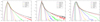 |
Fig. B.1. PDFs as functions of reduced densities ν = δ/σ, smoothed with different methods. Left and central panels show simulation L1024.1 smoothed with a B3 spline and the cubic-cell method, respectively, using a smoothing kernel length R = 4 h−1 Mpc. Right panel: Simulation L256.2 smoothed with the top-hat method with a kernel R = 2 h−1 Mpc. The smoothing rank is the first index in the simulation name, and the redshift is the second index. Colours indicate the evolutionary epoch z = 30, 10, 5, 3, 1, and 0. The dashed bold curves show the Gaussian distribution. |
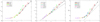 |
Fig. B.2. Mathematical kurtosis K(σ) of simulation L256 using various smoothing algorithms. Left panel: Results for smoothing with a B3 spline. Central panel: Results with a cubic-cell smoothing. Right panel: Results for the kurtosis M4 = K + 3 using a top-hat smoothing. The name index shows the redshift. The dashed bold curves show K = 16σ2. |
All Tables
All Figures
|
Fig. 1. Density fields of simulation L256 without additional smoothing and with a smoothing length 8 h−1 Mpc are shown in the upper and bottom panels, respectively. The panels from left to right show fields for epochs z = 30, z = 10, z = 3, and z = 0, presented in slices of size 200 × 200 × 0.5 h−1 Mpc. Only over-density regions are shown with colour scales from left to right 1−1.4, 1−2, 1−4, and 1−8 in the upper panels and 1−1.08, 1−1.25, 1−1.8, and 1−5 in the lower panels. |
| In the text | |
|
Fig. 2. Density distribution functions P(δ) as functions of the DM density contrast δ normalised to the rms of density fluctuations ν = δ/σ for simulation L1024 smoothed with the cubic-cell method. Panels from left to right: smoothing lengths Rt = 4, 8, 16 h−1 Mpc, indicated as the first index in the simulation name and the redshift coded in the second index. Dashed curves show the Gaussian distribution. |
| In the text | |
|
Fig. 3. Dependence of the PDF moments on the cosmic epoch z for simulation L512. Left top and bottom panels: dependence for the skewness S(z) and the kurtosis K(z), respectively, and right panels: their cosmological equivalents S3(z) and S4(z). The index in the simulation name is the smoothing length in h−1 Mpc. |
| In the text | |
|
Fig. 4. Mean logarithmic gradients for the redshift range 0 ≤ z ≤ 30 of the skewness, ⟨γS⟩, and the kurtosis, ⟨γK⟩, as functions of the smoothing length, Rt. Open symbols show the skewness S, and filled symbols show the kurtosis K. For clarity, the symbols for simulations L256 and L1024 are slightly shifted in Rt coordinate. |
| In the text | |
|
Fig. 5. Top panels: evolutionary tracks. Bottom panels: evolutionary diagrams. Left panels: skewness S. Right panels: kurtosis K. In the evolutionary tracks, the symbols along the tracks from left to right are for redshifts z = 30, 10, 5, 3, 1, and 0. In the evolutionary diagrams, the symbols from top to bottom correspond to smoothing lengths 2, 4, 8, and 16 h−1 Mpc. The solid bold black curves show the skewness S(σ) and kurtosis K(σ) according to the log-normal distribution. The dashed curves show S = 3σ and K = 16σ2. |
| In the text | |
|
Fig. 6. Top panels: evolutionary tracks. Bottom panels: evolutionary diagrams. Left panels: skewness S3. Right panels: kurtosis S4. In the evolutionary tracks, the symbols along the tracks from the left are for redshifts z = 30, 10, 5, 3, 1, and 0. In the evolutionary diagrams, the symbols from top to bottom correspond to smoothing lengths 2, 4, 8, and 16 h−1 Mpc. The solid black curves show the cosmological skewness S3 and kurtosis S4 according to the log-normal distribution. The dotted curves show the predictions of the perturbation theory Eq. (11). |
| In the text | |
|
Fig. 7. Top panels: evolutionary tracks. Bottom panels: evolutionary diagrams. Left panels: skewness S3. Right panels: kurtosis S4. The shaded areas correspond to the 1σ statistical uncertainties. |
| In the text | |
|
Fig. 8. Maxima of the skewness S3 and kurtosis S4 evolutionary tracks as functions of the smoothing length Rt. Open symbols show the skewness S3 and filled symbols show the kurtosis S4 for GADGET simulations of various cube lengths L0. The black and red curves show the maxima of the S3 and S4 curves of the GLAM simulations. |
| In the text | |
|
Fig. 9. Comparison of the PDFs with the same rms fluctuations σ = 0.8, but estimated at different redshifts z = 0 and z = 5. The PDFs are scaled with δ3 to reduce the dynamical range. The filtering scales are Rt = 10 h−1 Mpc at z = 0 and Rt = 0.5 h−1 Mpc at z = 5. |
| In the text | |
|
Fig. 10. Comparison of S3(σ, z) for redshifts z = 0, 1, and 5 found in N-body simulations with the predictions of the PT, Eq. (11), and the log-normal distribution, Eq. (14). |
| In the text | |
|
Fig. A.1. Shape of the box spline kernel B3. The solid curve shows the B3(x) kernel, and the dashed curve shows a Gaussian with σ = 0.6. |
| In the text | |
|
Fig. A.2. Comparison of simulation power spectra with the corresponding linear spectra and non-linear HALOFIT results at various epochs z. |
| In the text | |
|
Fig. B.1. PDFs as functions of reduced densities ν = δ/σ, smoothed with different methods. Left and central panels show simulation L1024.1 smoothed with a B3 spline and the cubic-cell method, respectively, using a smoothing kernel length R = 4 h−1 Mpc. Right panel: Simulation L256.2 smoothed with the top-hat method with a kernel R = 2 h−1 Mpc. The smoothing rank is the first index in the simulation name, and the redshift is the second index. Colours indicate the evolutionary epoch z = 30, 10, 5, 3, 1, and 0. The dashed bold curves show the Gaussian distribution. |
| In the text | |
|
Fig. B.2. Mathematical kurtosis K(σ) of simulation L256 using various smoothing algorithms. Left panel: Results for smoothing with a B3 spline. Central panel: Results with a cubic-cell smoothing. Right panel: Results for the kurtosis M4 = K + 3 using a top-hat smoothing. The name index shows the redshift. The dashed bold curves show K = 16σ2. |
| In the text | |
Current usage metrics show cumulative count of Article Views (full-text article views including HTML views, PDF and ePub downloads, according to the available data) and Abstracts Views on Vision4Press platform.
Data correspond to usage on the plateform after 2015. The current usage metrics is available 48-96 hours after online publication and is updated daily on week days.
Initial download of the metrics may take a while.