| Issue |
A&A
Volume 652, August 2021
|
|
|---|---|---|
| Article Number | A85 | |
| Number of page(s) | 12 | |
| Section | The Sun and the Heliosphere | |
| DOI | https://doi.org/10.1051/0004-6361/202039821 | |
| Published online | 13 August 2021 | |
Effects of the chromospheric Lyα line profile shape on the determination of the solar wind H I outflow velocity using the Doppler dimming technique
1
Dipartimento di Fisica e Astronomia “Ettore Majorana” – Sezione Astrofisica, Università degli Studi di Catania, Via S. Sofia 78, 95123 Catania, Italy
e-mail: This email address is being protected from spambots. You need JavaScript enabled to view it.
2
INAF – Osservatorio Astrofisico di Catania, Via S. Sofia 78, 95123 Catania, Italy
3
INAF – Osservatorio Astrofisico di Torino, Via Osservatorio 20, 10025 Pino Torinese, TO, Italy
4
INAF – Osservatorio Astrofisico di Capodimonte, Salita Moiariello 16, 80131 Napoli, Italy
5
CNR – Istituto di Fotonica e Nanotecnologie, Via Trasea 7, 35131 Padova, Italy
6
Dipartimento di Fisica e Astronomia, Università degli Studi di Firenze, Largo Enrico Fermi 2, 50125 Firenze, Italy
Received:
31
October
2020
Accepted:
5
May
2021
Abstract
Context. The determination of solar wind H I outflow velocity is fundamental to shedding light on the mechanisms of wind acceleration occurring in the corona. Moreover, it has implications in various astrophysical contexts, such as in the heliosphere and in cometary and planetary atmospheres.
Aims. We aim to study the effects of the chromospheric Lyα line profile shape on the determination of the outflow speed of coronal H I atoms via the Doppler dimming technique. This is of particular interest in view of the upcoming measurements of the Metis coronagraph aboard the Solar Orbiter mission.
Methods. The Doppler dimming technique exploits the decrease of coronal Lyα radiation in regions where H I atoms flow out in the solar wind. Starting from UV observations of the coronal Lyα line from the Solar and Heliospheric Observatory (SOHO), aboard the UltraViolet Coronagraph Spectrometer, and simultaneous measurements of coronal electron densities from pB coronagraphic observations, we explored the effect of the profile of the pumping chromospheric Lyα line. We used measurements from the Solar UV Measurement of Emitted Radiation, aboard SOHO, the Ultraviolet Spectrometer and Polarimeter, aboard the Solar Maximum Mission, and the Laboratoire de Physique Stellaire et Planetaire, aboard the Eight Orbiting Solar Observatory, both from representative on-disc regions, such as coronal holes and quiet Sun and active regions, and as a function of time during the solar activity cycle. In particular, we considered the effect of four chromospheric line parameters: line width, reversal depth, asymmetry, and distance of the peaks.
Results. We find that the range of variability of the four line parameters is of about 50% for the width, 69% for the reversal depth, and 35% and 50% for the asymmetry and distance of the peaks, respectively. We then find that the variability of the pumping Lyα profile affects the estimates of the coronal H I velocity by about 9−12%. This uncertainty is smaller than the uncertainties due to variations of other physical quantities, such as electron density, electron temperature, H I temperature, and integrated chromospheric Lyα radiance.
Conclusions. Our work suggests that the observed variations in the chromospheric Lyα line profile parameters along a cycle and in specific regions negligibly affect the determination of the solar wind speed of H I atoms. Due to this weak dependence, a unique shape of the Lyα profile over the solar disc that is constant in time can be adopted to obtain the values of the solar wind H I outflow velocity. Moreover, the use of an empirical analytical chromospheric profile of the Lyα, assumed uniform over the solar disc and constant in time, is justifiable in order to obtain a good estimate of the coronal wind H I outflow velocity using coronagraphic UV images.
Key words: Sun: chromosphere / Sun: corona / Sun: UV radiation / solar wind
© ESO 2021
1. Introduction
The solar wind is a tenuous plasma that continuously escapes from the Sun into the interplanetary medium. It extends for thousands of millions of kilometers and is mainly characterised by a fast component, with typical velocities of about 500−800 km s−1 flowing from coronal holes (CHs), and a slow component, with typical velocities of about 300−500 km s−1, mainly related to the streamer belt regions (see e.g. McComas et al. 1998, 2008).
The high coronal temperatures, of which the origin is still unclear, cause wind expansion (e.g. Parker 1958) and eventually the acceleration of slow and fast solar wind. It is thought that such acceleration could be the result of, for example, energy dissipation through the ion cyclotron resonance of high-frequency left-hand polarised Alfvén waves (see e.g. Ofman 2010).
Given the high coronal temperatures, the solar wind is mainly composed of fully ionised hydrogen and helium and of free electrons. The latter component is mainly observed through the scattering and polarisation of the white light coming from the photosphere (Thomson scattering). Other ions of heavier minor elements are present in smaller amounts.
The ESA/NASA Solar and Heliospheric Observatory (SOHO; Domingo et al. 1995) spacecraft returned a wealth of data, which provided a new understanding of the physical phenomena that contribute to the acceleration of the solar wind in the corona. In particular, the UltraViolet Coronagraph Spectrometer (UVCS; Kohl et al. 1995) on board SOHO allowed us to obtain crucial results, such as information on elemental abundances and kinetic temperatures of H I and O VI ions in different coronal structures. Antonucci et al. (2005), Susino et al. (2008), and Abbo et al. (2010) suggested that the main source of the slow solar wind is the boundary region between CHs and streamers, where the wind is dependent on the magnetic field topology. Outflows from active regions (ARs) could even contribute to the slow wind component (Zangrilli & Poletto 2016). The presence of pseudo or unipolar streamers can also contribute to the slow solar wind. Furthermore, white light observations with the Large Angle and Spectrometric COronagraph (LASCO; Brueckner et al. 1995) aboard SOHO have shown that outflows are connected to both large-scale ‘streamer blowout’ structures, the coronal mass ejections (CMEs) closely associated with magnetic reconnection at the current sheet above the cusp of the streamers, and to small-scale inhomogeneities (blobs), linked to quasi-periodic emission of plasma from cusps of helmet streamers (Sheeley et al. 1997; Wang et al. 1998; Song et al. 2009; Viall & Vourlidas 2015; see also the review of Abbo et al. 2016).
Generally, observations of emission lines in the off-limb corona, such as the H I Lyα (121.6 nm), which are mainly due to scattering processes of radiation coming from the low solar atmosphere, can be used to determine the radial component of the outflow velocity (vw) of the specific atom or ion that generates the scattering through the Doppler dimming technique (Hyder & Lites 1970; Withbroe et al. 1982; Noci et al. 1987). This technique consists of the analysis of the intensity decrease of the coronal ultraviolet (UV) radiation coming from flowing regions, and it relies on some assumptions and prior knowledge of the geometrical and physical properties that are representative of the coronal environment (such as electron density, electron temperature, and kinetic temperature of the scattering ions) and of the source of the UV radiation scattered (such as intensity and line profile of the exciting chromospheric radiation). However, in those cases in which observations come from coronagraphs designed for imaging only, these quantities cannot be directly determined and they must be taken from the literature. Critical works aimed at investigating how the choice of the parameters adopted from the literature (and their uncertainties) or from specifically constructed databases may affect the results of the Doppler-dimming analysis have been presented very recently.
In this context, Dolei et al. (2016) analysed the H I Lyα line profiles observed by UVCS instrument in a number of polar, mid-latitude, and equatorial structures. They considered a large amount of data acquired in a time range longer than a complete solar cycle (1996–2012) and determined the temperature components for neutral hydrogen at different phases of solar activity. They were able to derive the H I temperature radial profiles for several heliocentric distances (from 1.3 R⊙ to 4.5 R⊙) and polar angles.
Dolei et al. (2018) used coronagraphic Lyα observations from UVCS and visible light (VL) images obtained with LASCO and the Mark-III Coronameter (Mk3/MLSO; Fisher et al. 1981) to study the dependence of the derived solar wind H I outflow velocity on the physical parameters that characterise the scattered coronal Lyα emission when the Doppler dimming effect is considered. They found that the electron temperature has the most important impact on the determination of the H I outflow velocity, while the coronal H I temperature has an important role at larger heliocentric distances, where higher speeds are reached.
Dolei et al. (2019) also used UVCS and LASCO-Mk3 observations in order to analyse the effect of chromospheric radiation inhomogeneities on the solar wind H I outflow velocity determination with respect to the case in which a uniform-disc brightness approximation is adopted. In particular, they created a Carrington map of the non-uniform solar chromospheric Lyα radiation using a correlation function between the H I 121.6 nm and He II 30.4 nm intensities (Auchère 2005), while some approximations concerning the coronal H I temperature and a constant value of the radiance over the entire solar disc were adopted for the uniform-disc brightness case. They found that the uniform condition leads to an overestimated velocity of 50−60 km s−1 in polar and mid-latitude regions, while underestimated velocity values are obtained at the equatorial regions. This difference decreases at higher altitudes.
The present work can be considered as a step forward in the investigations carried out by Dolei et al. (2018, 2019). The aim of this paper is to study the effects induced on the determination of the solar wind H I velocity by the variation of the exciting chromospheric Lyα line profile shape, which can occur among different regions on the solar surface, such as quiet or active regions and CHs, or during different phases of the solar activity cycle. For this purpose, we considered Lyα chromospheric observations performed by the Solar UV Measurement of Emitted Radiation (SUMER; Wilhelm et al. 1995) aboard the SOHO spacecraft, which include full disc observations (Lemaire et al. 2015) and the best sets of Lyα solar-disc observations currently available (Curdt et al. 2008; Tian et al. 2009a,b). We also considered other observations concerning ARs, quiet Sun (QS) regions, and an equatorial CH performed by the Ultraviolet Spectrometer and Polarimeter (UVSP; Miller et al. 1981) aboard the Solar Maximum Mission (SMM; Woodgate et al. 1980) and the Laboratoire de Physique Stellaire et Planetaire instrument (LPSP; Artzner et al. 1977; Bonnet et al. 1978) aboard the Eight Orbiting Solar Observatory (OSO-8). Other parameters critically affecting the coronal Lyα emission, such as the electron temperature, the electron density, and the neutral hydrogen temperature, are the same as those adopted by Dolei et al. (2019).
In order to facilitate the comparison, bidimensional (2D) maps of outflow solar wind H I velocity were produced by using the same numerical code as in Dolei et al. (2018, 2019), based on the reproduction of the synthetic coronal Lyα intensity along the line of sight (LOS). The numerical computations have allowed us to change the value of the wind velocity vw until a match with the observed coronal intensity is reached. Moreover, this allowed us to estimate the solar wind velocity as a function of heliocentric distance and latitude. In obtaining each map of solar wind H I outflow velocity, we assumed that the chromospheric intensity and the line profile of the Lyα emission are unique over the entire solar disc.
Our study is of particular interest for the analysis and interpretation of coronal Lyα observations that will be obtained by the Metis coronagraph (Antonucci et al. 2020; Fineschi et al. 2020) onboard the Solar Orbiter spacecraft (Müller & Marsden 2013; Müller et al. 2020). Indeed, Metis, which is designed for imaging only, observes linearly polarised VL (580 nm−640 nm) and UV Lyα emission at the same time with a field of view (FOV) that ranges from 1.6 R⊙ to 7.5 R⊙ (Antonucci et al. 2020), viewing the Sun from latitudes up to about 30° with respect to the equatorial plane (Zouganelis et al. 2020).
In Sect. 2, the main mechanisms concerning the coronal emission, the analysis technique used, and the observations are described. Section 3 is dedicated to the obtained results. Finally, in Sect. 4, we discuss the results and give our conclusions.
2. Data analysis
2.1. Mechanisms of coronal emission and the Doppler dimming phenomenon
In a static corona, the emission coming from coronal atoms/ions is due to the excitation induced by two main mechanisms: the collision with free electrons and the resonant scattering of chromospheric radiation. However, in the case of the H I Lyα emission, the collisional term contributes only to a small fraction of the total coronal emission (Gabriel 1971; Raymond et al. 1997, Landi Degli’Innocenti; priv. comm., quoted in Noci et al. 1987), given the stronger dependence of the collisional component ℐcol of the coronal intensity on the electron column density Ne (i.e.  ) with respect to the resonant one ℐrad (i.e. ℐrad ∝ Ne; see e.g. Withbroe et al. 1982) and the low-density conditions present in the outer corona. For this reason, it can be neglected.
Under the hypothesis of low-density coronal plasma, the radiance ℐrad (in units of erg cm−2 s−1 sr−1) coming from H I atoms in a coronal point P and measured along the n direction, corresponding to the line of sight, can be expressed by the following:
 (1)
(1)
where h is the Planck constant; B12 is the Einstein coefficient for the Lyα transition; λ0 = 121.567 nm is the central wavelength of the considered transition; ne is the electron density; 0.833 is the ratio between proton and electron density for a gas that is completely ionised and contains 10% helium; Te is the electron temperature; RH I(Te) is the total hydrogen ionisation fraction as a function of Te, meaning the ratio between the neutral hydrogen and proton density (see e.g. Withbroe et al. 1982); dl is the infinitesimal path along the line of sight; n′ is the direction along which the chromospheric radiation reaches the coronal point P; Ω is the solid angle under which the point P subtends the solar disc (see e.g. Fig. 1 in Dolei et al. 2015); p(Ω) = [11 + 3(n ⋅ n′)2]/[12 (4π)] is a geometrical factor that gives the angular dependence of the scattering process (see Beckers & Chipman 1974); and
 (2)
(2)
is the convolution between the chromospheric specific intensity I(λ′−λ0 − δλ, n′) and the normalised coronal absorption profile Φ(λ′−λ0), where λ′ is the wavelength. The term
 (3)
(3)
is the Doppler shift seen along n′ by the scattering atoms due to the velocity v (supposed radially symmetric) of the scattering atoms, where vw is the module of v, θ is the angle between v and n′, and c is the speed of the electromagnetic radiation in the vacuum (see Fig. 1 in Dolei et al. 2015 for a clear description of the geometry of the scattering process). The specific intensity I(λ′−λ0 − δλ, n′) = I(n′)⋅Ψ(λ′−λ0 − δλ) is the product between the radiance I(n′) (in units of erg cm−2 s−1 sr−1) and the normalised intensity profile Ψ(λ′−λ0 − δλ) (in units of Å−1) of the chromospheric Lyα line. Then, F(n′, vw, θ) gives information about the dependence on the H I atom’s velocity of the radiative excitation efficiency by chromosperic radiation. If we assume that the velocity distribution of the absorbing H I coronal atoms is Maxwellian, the normalised coronal absorption profile Φ(λ′−λ0) has a width that depends on the thermal motion only (neglecting all contributions coming from non-thermal phenomena, such as turbulence, waves, oscillations, and so on), given by
 (4)
(4)
where kB is the Boltzmann constant, TH I is the H I temperature, and mH is the mass of hydrogen atoms.
We also define the ‘Doppler factor’ D(vw) (see Noci et al. 1987):
 (5)
(5)
which accounts for the overlapping between the coronal absorption profile and the exciting chromospheric one as a function of vw.
When the radiative resonantly scattered emission dominates, the outwards expansion of the corona generates a decrease (dimming) in the Lyα coronal emission. This phenomenon can be explained considering the Doppler redshift which an observer positioned in P measures in the chromospheric radiation. In fact, when the corona is in a static condition, the profile of the chromospheric Lyα is centred at λ0, causing the maximum intensity of the scattered Lyα radiation (D = 1). However, when the corona is expanding, the scattered Lyα is dimmed because of the Doppler shift of the chromospheric photons seen by the outflowing coronal H I atoms. The intensity of the scattered radiation tends to vanish when the outflow velocity becomes higher, because the chromospheric and coronal profiles no longer overlap (D ≈ 0). Thus, it is possible to match the synthetic intensity ℐrad and that measured by observations by numerically tuning the vw value, estimating in turn the outflow velocity.
2.2. Observations
We describe the observations adopted in our analysis here.
2.2.1. UV and pB observations
A synoptic UV map related to the observations of coronal Lyα intensity and analysing data acquired on June 7, 1997 (during the minimum of solar activity) by UVCS was obtained. This 2D map was constructed, as explained by Bemporad (2017) and Dolei et al. (2018), starting from synoptic UVCS observations and by performing a power-law interpolation of intensities observed at different latitudes and altitudes. A polarised brightness pB map in visible light was obtained by interpolating observations acquired with Mk3 between 1.1 R⊙ and 1.5 R⊙ and by LASCO above 2.5 R⊙ on the same day (see Bemporad 2017; Dolei et al. 2018, for more details). The maps, which are shown in Fig. 1, are those considered in the work by Dolei et al. (2019).
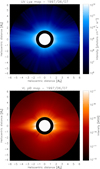 |
Fig. 1. Bidimensional maps of UV coronal Lyα intensity (top panel), acquired by UVCS/SOHO, and VL pB emission (bottom panel), obtained from combined observations by the LASCO/SOHO and Mk3/MLSO instruments as a function of heliocentric distance and latitude. The maps have a FOV between 1.5 R⊙ and 6.0 R⊙, and refer to observations taken on June 7, 1997. |
It is worth mentioning that we only considered coronal observations related to the minimum solar activity, although the analysed chromospheric observations, as described below, concern an entire solar cycle. However, since the aim of this work is to investigate the effects induced by the chromospheric Lyα profile shape variation on the H I outflow velocity, it is not unreasonable to adopt a simplified scenario.
2.2.2. Chromospheric observations of Lyα line profiles
In this study, we aim to explore the impact of possible variations in the spectral profile of the pumping chromospheric radiation, such as those caused by the solar activity cycle, on the determination of vw. For this purpose, we considered full disc, QS and CH observations of the chromospheric Lyα line profiles carried out by SUMER/SOHO during the solar activity cycle 23, ARs and QS profiles acquired by UVSP/SMM, and profiles referring to an equatorial CH and a flare acquired by the LPSP instrument aboard OSO-8, in order to take into account all the possible chromospheric regions emitting the exciting radiation.
First, we used measurements of the Lyα line profile relative to the entire solar disc. These were provided by Lemaire et al. (2015) and are available at the Centre de Données astronomiques de Strasbourg (CDS)1. These data, comprising 43 profiles, do not provide information about possible variations of the chromospheric Lyα profile between different regions on the solar surface observed at the same time. Nevertheless, since they cover an entire solar cycle, it is reasonable to expect that a good indication of the effect of the solar activity level on the shape of the chromospheric Lyα line can be achieved, at least in the coronal equatorial regions.
Lyα profiles observed by SUMER in different areas of the solar disc (Curdt et al. 2008; Tian et al. 2009a,b) represent the best Lyα solar-disc observations currently available. We considered two profiles observed on September 23, 2008 and on April 17, 2009, which are relevant to a QS region at the disc centre and to a CH observed at the south pole, respectively (for more details, see Tian et al. 2009a,b).
The UVSP profiles considered in this work were reported by Fontenla et al. (1988) in their Figs. 3, 5, 6, and 12, where the geocoronal absorption was removed, while the LPSP instrument on OSO-8 profiles were acquired in an equatorial CH at the central meridian between 27 and 29 November, 1975 (Bocchialini & Vial 1996) and in a faint flare that occurred in an AR observed on April 15, 1978 (Lemaire et al. 1984). Analytic fits to chromospheric Lyα profiles were also taken into account. In order to examine the variation of each parameter of the Lyα line profile (line width, reversal depth, asymmetry of the peaks, and separation of the peaks), we selected four couples of profiles, each of them representing extreme cases of the considered profile parameters. In Table 1, we report these four couples, determined as described in the following. However, we ensured that all the extreme cases analysed were represented by using only the five observed profiles shown in panel a of Fig. 2, where each of them has been normalised to its own total intensity.
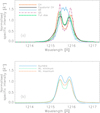 |
Fig. 2. Panel a: Lyα irradiance profiles reported in Figs. 6a and 12 of Fontenla et al. (1988; QS and AR, respectively), as well as profiles observed on April 17, 2009 (CH, Tian et al. 2009b), on October 28, 1996 (full disc, Lemaire et al. 2015) and in an equatorial CH at the central meridian between November 27 and 29, 1975 (Bocchialini & Vial 1996). Panel b: parametrised Lyα profiles from Kowalska-Leszczynska et al. (2018; IKL; at maximum and at minimum) and Auchère (2005). Each profile has been normalised to its total intensity. |
Four couples of selected observed profiles representing the extreme cases of the considered profile parameters.
We measured the full width at half maximum (FWHM) of each selected Lyα chromospheric profile once these were normalised to their total intensities. The mean value of the two peaks’ highest intensities was adopted as the maximum intensity of the Lyα line profile. Its half value was then used to calculate the FWHM of the line. Only in the case of the considered profile without reversal, meaning that relative to AR 2340 and reported in Fig. 12 of Fontenla et al. (1988), did we obtain the FWHM by performing a Gaussian fit.
We find a difference between the line widths of about 50% at most over the entire cycle, with respect to the narrowest observed Lyα chromospheric profile. It is worth noting that we did not find evidence of a correlation of the variation of the line widths with the solar cycle. Indeed, the two line profiles that exhibit the largest difference between their FWHMs correspond to that observed on April 17, 2009 (CH) and that reported in Fig. 12 of Fontenla et al. (1988; AR 2340), respectively. These profiles are shown in panel a of Fig. 2 and in Fig. 3 (red dashed line and blue solid line, respectively). They are considered extreme cases with regard to the line profile width.
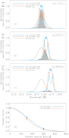 |
Fig. 3. Panels a–c: normalised chromospheric profiles reported in Fig. 12 of Fontenla et al. (1988; AR 2340, blue solid line) and observed on April 17, 2009 (red dashed line; Tian et al. 2009b), overlapped with a normalised Gaussian coronal absorption profile (black dotted line) computed by setting the coronal H I temperature to 1.5 × 10⁶ K, considering θ = 0°. Panels a–c: correspond to outflow velocities equal to vw = 0 km s−1, vw = 150 km s−1, and vw = 300 km s−1, respectively. In the case of the exciting narrowest profile, we also display the grey shaded area that is proportional to the product of the coronal absorption profile (Φ) and the chromospheric pumping profile (Ψ). Panel d: Doppler factor as a function of vw calculated considering each chromospheric profile (AR 2340: blue solid line; polar CH: red dashed line). Triangles, squares and asterisks indicate the Doppler dimming values corresponding to H I outflow velocities equal to vw = 0 km s−1, vw = 150 km s−1, and vw = 300 km s−1, respectively. |
The shallowest and the deepest profiles in terms of reversal depth are those described in Fig. 12 (AR 2340, showing a negligible reversal) and Fig. 6a (QS) of Fontenla et al. (1988), respectively. The depth was calculated by considering the minimum central intensity value of the profile and dividing this by the mean value between the maximum peak intensities. The reversal depth variation of the deepest profile is equal to about 69% with respect to the shallowest one. These profiles, representing the extreme cases related to the profile reversal depth, are displayed in panel a of Fig. 2 (blue solid line and magenta dash-dot-dot-dot line, respectively).
The peak-to-peak asymmetry between the peaks of each profile was measured by considering the ratio I peak − blue/I peak − red. The profile with the largest difference between the maximum peak intensities is that observed on October 28, 1996 (full disc), which exhibits the highest blue asymmetry (I peak − blue/I peak − red = 1.16). This profile is displayed in panel a of Fig. 2 and in panel c of Fig. 4 (green dash-dotted line).
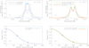 |
Fig. 4. Panel a: normalised shallowest (blue solid line) and deepest (magenta dash-dot-dot-dot line) profiles described in Figs. 6a and 12 of Fontenla et al. (1988), respectively, overlapped with a normalised Gaussian coronal profile (black dotted line) computed by setting the coronal H I temperature at 1.5 × 10⁶ K, considering θ = 0°. Panel b: Doppler factor as a function of vw calculated considering each chromospheric profile. Triangles, squares, and asterisks: see Fig. 3. Panels c and d: same as in panels a and b, but concerning the bluest asymmetric profile (I peak − blue/I peak − red = 1.16) observed on October 28, 1996 (green dash-dotted line; Lemaire et al. 2015) and the reddest asymmetric profile (I peak − blue/I peak − red = 0.86; red solid line), respectively. |
Moreover, to study the effects induced by the asymmetry of the peaks on the H I outflow velocity, we also took into account the synthetic and reddest asymmetric profile (I peak − blue/I peak − red = 0.86), which was obtained by taking the opposite of the bluest asymmetric profile (characterised by the ratio I peak − blue/I peak − red = 1.16), which is the one observed on October 28, 1996 (full disc). This profile is shown in panel c of Fig. 4 (red solid line).
The line profiles with the largest and smallest peak separations are those observed on April 17, 2009 (polar CH) and in the equatorial CH at the central meridian on 27−29 November, 1975, respectively. The separation variation is equal to about 50% with respect to the smallest separation value. The profiles are shown in panel a of Fig. 5 (red dotted line and green solid line, respectively).
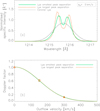 |
Fig. 5. Panel a: normalised CH profiles with smallest (green solid line) and greatest (red dashed dotted line) peak separations observed in an equatorial CH at the central meridian on 27−29 November, 1975 (Bocchialini & Vial 1996), and on April 17, 2009 (polar CH; Tian et al. 2009b), respectively, overlapped with a normalised Gaussian coronal profile (black dotted line) computed by setting the coronal H I temperature at 1.5 × 10⁶ K, considering θ = 0°. Panel b: Doppler factor as a function of vw calculated considering each chromospheric profile. Triangles, squares, and asterisks: see Fig. 3. |
We also compared two different profiles relative to ARs. The first one, reported in Fig. 5a of Fontenla et al. (1988; AR 2363), shows a remarkable reversal, while the second one, shown in Fig. 12 of Fontenla et al. (1988; AR 2340), is characterised by a negligible reversal. In addition, we analysed the characteristic Lyα profile of a faint flare observed in an AR, which is reported in Fig. 1 of Lemaire et al. (1984), comparing it to the profile of AR 2340.
Furthermore, we considered the analytic expression for the Lyα irradiance profile proposed by Auchère (2005) and also used by Dolei et al. (2018, 2019), together with two cases of the parametrised profile reported in Kowalska-Leszczynska et al. (2018, hereafter referred to as IKL). The first one consists of a sum of three Gaussian components, which was introduced to reproduce the mean Lyα observed profile at solar minimum. The other two profiles were constructed by taking into account the sum of a k-function, a straight line that simulates the background, and a reversal Gaussian function reproducing the line reversal. Such profiles were calculated for both the maximum and minimum irradiance values reported in Table A.1 of Lemaire et al. (2015). These profiles are presented in panel b of Fig. 2 (Auchère: blue solid line; IKL at minimum: green dashed line; IKL at maximum: red dash-dotted line).
In order to calibrate the radiance of the spectral data from SUMER, we considered the absolute values of line radiance I (erg cm−2 s−1 sr−1) provided by the SOLar STellar Irradiance Comparison Experiment (SOLSTICE; Rottman & Woods 1994) aboard the Upper Atmosphere Research Satellite (UARS; Reber 1990), as explained, for example, in Lemaire et al. (1998, 2002, 2015). The solid angle subtended by the solar disc at the distance of SOLSTICE (∼1 AU) was taken into account. The considered profiles were all normalised to the same value of absolute line radiance observed at the minimum, such as that acquired on May 22, 1997, which corresponds to the SUMER observation closest in time to the coronal Lyα map reconstructed from UVCS observations reported in this paper. This value is I = Imin = 8.59 × 10⁴ erg cm−2 s−1 sr−1 (see Table 1 of Lemaire et al. 2015).
2.3. Parameters for the synthesis of the Lyα scattered intensity
In order to estimate vw, we synthesised the intensity of the coronal Lyα to be compared with UVCS observations using the code described in Dolei et al. (2018, 2019). For the computation of the synthetic coronal emission, we need information about the physical quantities on which the Lyα intensity depends, such as ne, Te, and TH I, under some assumptions and approximations.
The electron density ne is obtained through the inversion method developed by Van De Hulst (1950) that describes the polarised brightness (due to the Thomson scattering) as dependent only on the electron density, under the hypothesis of cylindrical symmetry (see, e.g., Hayes et al. 2001; Dolei et al. 2015). We used the profile of ne derived from the LASCO pB map, as described in Dolei et al. (2018).
For the electron temperature Te, we used the values derived by Dolei et al. (2019). They obtained Te as a function of the heliocentric distance and latitude, taking into account the dependence found by Gibson et al. (1999) for equatorial regions and by Vasquez et al. (2003) for high latitude regions, under the hypothesis of super-radial expansion of the solar wind in polar CHs during the solar minimum. Interpolated values for mid latitudes have been used.
The H I temperature comes from the database created by Dolei et al. (2016). We considered a TH I map for a solar minimum epoch, following Dolei et al. (2019). In order to fit the neutral hydrogen temperature profile and to create a 2D map as a function of latitude and heliocentric distance, the functional form given by Vasquez et al. (2003) was used, as in Dolei et al. (2016). It is worth mentioning that the values of TH I are likely overestimated, because the hydrogen line broadening includes contributions due to non-thermal mechanisms.
For the sake of simplicity, we adopted the approximation θ = 0°, that is, v ∥ n′ in all the computations leading to the results described in Sect. 3. However, the consequence of assuming values of θ ≠ 0 on the inferred values of the H I outflow velocities has been evaluated as a separate step and is also described in Sect. 3.
3. Results
In order to verify the effects of the chromospheric Lyα profile shape on the determination of the solar wind H I velocity, we first studied the behaviour of the Doppler factor dependent on the profile width. The results are summarised in Fig. 3. The first three panels show the overlapping between the narrowest and broadest chromospheric profiles and the coronal one that has been calculated by assuming a H I temperature in the corona equal to 1.5 × 10⁶ K. We took into account the following velocity values: vw = 0 km s−1 (panel a), vw = 150 km s−1 (panel b), and vw = 300 km s−1 (panel c). In addition, for the case of the narrowest profile, we also display the grey shaded area that is proportional to the integrand value of the function F(n′, vw, θ) (see Eq. (2)). This quantity is closely related to the Doppler factor as it gives the overlapping between the coronal absorption profile (Φ) and the chromospheric pumping profile (Ψ).
In Fig. 3, panel d, the corresponding values of D(vw) are properly labelled on the curves, where the Doppler factor as a function of vw (varying from vw = 0 km s−1 to vw = 500 km s−1) is reported. We note that the curves in the bottom panel show a small difference between them, indicating that the Doppler dimming does not have a strong dependence on the variation of the line width of the selected chromospheric profiles.
We studied the Doppler factor D(vw) as a function of the profile reversal depth. The results are reported in Fig. 4. Panel a of Fig. 4 shows the overlapping of the coronal absorption profile with the shallowest and the deepest chromospheric profiles. The same analysis was carried out for the bluest and reddest asymmetric profiles (panel c of Fig. 4) and the profiles with the smallest and the largest separation between the peaks (panel a of Fig. 5). The curves in panels b and d of Fig. 4 and panel b of Fig. 5 do not show any significant differences between them. Therefore, the Doppler factor does not have a strong dependence on reversal depth, asymmetry, and separation of the peaks with regard to all the selected chromospheric profiles taken into account as extreme cases.
We performed a similar analysis by considering the three profiles reported in Fig. 2 (panel b). From Fig. 6 (panels a and b), we infer that the different parametrisations of these chromospheric profiles do not generate significant differences in the Doppler factor values, even if they are larger than in the observed profiles.
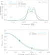 |
Fig. 6. Panel a: normalised parametrised chromospheric profiles reported in Fig. 2; Auchère (2005; blue solid line) and Kowalska-Leszczynska et al. (2018; green dashed line at minimum and red dot-dashed line at maximum), overlapped with a normalised Gaussian coronal profile (black dotted line) computed by setting the coronal H I temperature at 1.5 × 10⁶ K, considering θ = 0°. Panel b: Doppler factor relative to the profiles shown in panel a. Triangles, squares, and asterisks: see Fig. 3. |
A further analysis has been carried out for AR profiles. As shown in Fig. 7, when we compare the values of D(vw) for the AR 2363 (AR showing line reversal) and AR 2340 (AR with a negligible reversal), we find very small differences. Conversely, comparing the values relevant to the AR 2340 and the flare profiles, we observe significant differences.
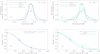 |
Fig. 7. Panel a: normalised AR profiles with and without reversal relevant to AR 2363 (magenta dash-dot-dot-dot line) and AR 2340 (blue solid line; see Fontenla et al. 1988), respectively, overlapped with a normalised Gaussian coronal profile (black dotted line) computed by setting the coronal H I temperature at 1.5 × 10⁶ K, considering θ = 0°. Panel b: Doppler factor as a function of vw calculated considering each chromospheric profile. Triangles, squares, and asterisks: see Fig. 3. Panels c and d: same as in panels a and b, but concerning the AR 2340 profile (blue solid line; Fontenla et al. 1988) and the normalised flare profile (green dash-dotted line; Lemaire et al. 1984), respectively. |
Furthermore, we performed a comparison considering different values of the angle between the flow and the line-of-sight directions, θ, using the Auchère profile. The results are shown in panel a of Fig. 8, where we can note that assuming different angles θ leads to the inference of remarkable variations of the H I outflow velocity values of about 14%.
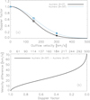 |
Fig. 8. Panel a: Doppler factor as a function of vw calculated considering the normalised Auchère (2005) profile when θ = 0° and θ = 30°. Triangles, squares, and asterisks: see Fig. 3. Panel b: absolute values of the outflow velocity differences determined considering the normalised Auchère (2005) profile when θ = 0° and θ = 30°, as a function of the Doppler factor. The top axis scale shows the velocity values corresponding to the Doppler factor values when the Auchère (2005) profile is taken into account and θ = 0°. |
To better understand these results, in Fig. 9 we plot the absolute value of the differences between the values of solar wind H I velocity corresponding to the same value of Doppler factor relative to the different chromospheric observed and parametrised profiles. It is possible to note that in the former case (observed profiles) the velocity differences are within a range of about 22 km s−1 when we take into account the extreme cases. In the latter (parametrised profiles), the differences are within 30 km s−1, except for values of D(vw) close to zero, where the indetermination in the outflow velocity is much higher. However, in both cases, up to values of D(vw)≈0.2, the relative velocity differences are below about 9% and 12%, respectively. A similar result was obtained by Dolei et al. (2015), who found that an uncertainty within the range of H I temperature measured by UVCS can return an error up to 10% on the determination of the theoretical coronal Lyα intensity, with an influence on the estimate of the H I outflow velocity up to ±10−20 km s−1. When we consider the cases reported in Fig. 7, AR profiles with and without reversal and a profile observed during a flare, we can see that for the left panels of Fig. 7 the velocity differences are below 10 km s−1, while for the right panels of Fig. 7 these values reach about 100 km s−1 (see also Fig. 9, panel c). Therefore, we find relative values of about 3% and 21%, respectively. In Fig. 8, panel b, concerning the Doppler factor curves relative to different values of θ, a similar result is shown. In this case, the absolute values of the differences between the velocities corresponding to the same value of Doppler factor are below 70 km s−1, with relative values up to about 14%.
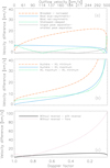 |
Fig. 9. Panel a: absolute values of the differences between the outflow velocity values determined with the different observed chromospheric profiles shown in Fig. 2 as a function of the Doppler factor. The abscissa axis is complemented with the velocity values corresponding to the Doppler factor in the case of the Auchère (2005) profile at the top of the panel. Panel b: same as in panel a, but with the parametrised chromospheric profiles shown in Fig. 2 and in panel a of Fig. 6. Panel c: same as in panel a, but taking into account the profiles shown in panels a and c of Fig. 7. |
Similarly to Dolei et al. (2016, 2018, 2019), we created 2D maps of the solar wind H I outflow velocity assuming the chromospheric Lyα line shape Ψ(λ) as the sole variable parameter, while all the other inputs were kept fixed. The maps have been created with a final FOV ranging from 1.5 R⊙ to 3.95 R⊙.
For a better visualisation of the variations induced by the use of different chromospheric line profile shapes, in Fig. 10 we report the results obtained in terms of the differences between the outflow velocity maps inferred from the various chromospheric profiles adopted: narrowest and broadest profiles (AR 2340 and SUMER April 17, 2009 CH, respectively; top left panel), narrowest and Auchère (2005) profiles (top right panel), broadest and Auchère (2005) profiles (bottom left panel), and narrowest and QS (SUMER, September 23, 2008) profiles (bottom right panel). These difference maps exhibit rms values equal to 18 km s−1, 19 km s−1, 20 km s−1, and 11 km s−1, respectively. As can be seen in Fig. 10, the differences are remarkable in the left panels. In particular, in the bottom left panel the differences are larger between about 1.5 R⊙ and 3.5 R⊙, only in the equatorial region.
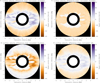 |
Fig. 10. Differences between solar wind H I outflow velocity maps obtained considering the narrowest profile (AR 2340; Fontenla et al. 1988) and the broadest one (polar CH – April 17, 2009; Tian et al. 2009b; top left panel), the narrowest and the Auchère (2005) analytic profiles (top right panel), the broadest and the Auchère (2005) analytic profiles (bottom left panel), and the narrowest profile with that observed on September 23, 2008 (QS; Tian et al. 2009b; bottom right panel). |
4. Discussion and conclusions
In this paper, we investigate the influence of the chromospheric Lyα line profile on the determination of the solar wind H I outflow velocity through the Doppler dimming technique (Hyder & Lites 1970; Noci et al. 1987; Withbroe et al. 1982).
In this analysis, we used spectroscopic measurements by SUMER (Lemaire et al. 2015; Curdt et al. 2008; Tian et al. 2009a,b), which include the data sets with the highest resolution of Lyα solar-disc observations presently available. We also selected some profiles of ARs and QS acquired by UVSP and described in Fontenla et al. (1988), where the correction concerning the geocoronal absorption was applied, along with a profile reported in Lemaire et al. (1984) characterising a solar flare, and another one acquired in an equatorial CH (Bocchialini & Vial 1996); both were obtained by the LPSP instrument on OSO-8. For the sake of completeness, it is worth recalling that the Chromospheric Lyman Alpha Spectropolarimeter (CLASP) observed the Sun in H I Lyα during a suborbital rocket flight in 2015 (Schmit et al. 2017). These observations measured the Lyα profile in a quiet-Sun target near the limb with a slit 400″ long and  wide. Overall, these observed profiles were in agreement with the early measurements of Gouttebroze et al. (1978), but they were affected by geocoronal absorption and water vapor contamination. Furthermore, SUMER measurements were recently used to derive a reference QS Lyα profile that would be representative of the Lyα radiation from the solar disc during a minimum solar activity (Gunár et al. 2020).
We analysed the behaviour of the Doppler factor with respect to the variation of four parameters on which the pumping Lyα profile depends: line width, reversal depth, asymmetry of the peaks, and separation of the peaks. Moreover, taking into account the same input data adopted by Dolei et al. (2019), that is, Te, TH I, ne, and the Lyα coronal intensity, and using a constant value for the radiance of the exciting chromospheric Lyα radiation, we computed outflow velocity maps, where the sole variable is the profile of the exciting chromospheric Lyα radiation.
It is worth mentioning that just recently Cranmer (2020) obtained radial profiles of electron and proton temperatures very different to those adopted in the present work. Since our main goal here is to investigate the effects of the chromospheric Lyα profile shape on the determination of the outflow velocity, we feel confident that the evaluation of Cranmer’s temperature profiles can be deferred to a future analysis without questioning the results obtained in the present work.
Considering chromospheric Lyα normalised profiles observed by SUMER, UVSP, and the LPSP instrument on OSO-8, we measured their FWHM, reversal depth, asymmetry of the peaks, and separation of the peaks. We found a maximum variation of about 50%, 69%, 35%, and 50% between the maximum and minimum values of each parameter on which the Lyα profile depends, respectively, referring each percentage to the minimum value of the corresponding parameter. Using these observations, we found that the Doppler factor D(vw), which is a measure of the overlapping between the coronal and chromospheric profiles as a function of the H I outflow velocity, does not strongly depend on the observed parameters that characterise the chromospheric Lyα profiles. In fact, except the case in which we consider a flare, the relative velocity differences determined using the different observed profiles, as a function of the Doppler factor, are below about 9%, a value that is comparable with the uncertainty in the velocity values determined by the Doppler dimming technique.
In order to further illustrate this effect, we also considered other analytic profiles, which were proposed by Auchère (2005) and Kowalska-Leszczynska et al. (2018). Also in these cases, we note negligible effects on the Doppler factor evaluation, obtaining relative absolute values of the velocity differences within a range of about 12% in correspondence of the same values of the Doppler factor. Conversely, non-negligible differences appear in the Doppler factor when we take into account a flare profile. In fact, in this case the resulting velocity variation is significantly larger, increasing up to about 100 km s−1 and returning a relative velocity difference values of about 21% (see Fig. 9, panel c).
We also show the effect of considering different values of the angle between the flow and the line-of-sight directions, θ. We find that if θ > 0°, the Doppler factor curve has a smoother trend than for θ = 0°. Figure 8 shows the case of θ = 30°. Therefore, when we consider a fixed value of the Doppler factor, the corresponding velocity value is greater when θ > 0°. However, the velocity differences remain below about 70 km s−1 in this case, with a relative value equal to ≈14%. It is worth mentioning that such a value for θ can be obtained only for very close distances from the Sun, of about 2 R⊙, so its contribution in the computation of the H I outflow velocity is limited; this remains more valid for higher values of θ.
We used the narrowest and the broadest profiles, the one observed on September 23, 2008 (QS), and the analytic profile deduced by Auchère (2005), to derive the 2D maps of H I outflow velocity. Taking into account the velocity difference maps shown in Fig. 10, we found that rms values of the difference of the solar wind H I speed are equal to 18 km s−1 (narrowest – broadest), 19 km s−1 (narrowest – Auchère), 20 km s−1 (broadest – Auchère), and 11 km s−1 (narrowest – QS). These values can be considered as possible uncertainties in the estimate of the outflow velocity with regard to the dependence on the chromospheric profile shape. However, they are significantly smaller than those found by Dolei et al. (2018), which are related to other parameters. In fact, assuming a maximum uncertainty on the other physical quantities of ±30%, they estimated that the resulting uncertainties on the derived velocity were of 67 km s−1, 67 km s−1, 81 km s−1, and 45 km s−1 for the impact of electron density, total chromospheric intensity, electron temperature, and H I temperature, respectively.
Therefore, our results indicate that even the largest variations actually observed in the parameters on which the chromospheric Lyα profile depends, related to the solar magnetic activity and to different disc regions, return small differences in the H I outflow velocity estimate, excluding the flare case, where non-negligible effects are present. This reveals how little effect the shape of the exciting chromospheric Lyα profile has on the determination of the solar wind H I outflow velocity with respect to the other parameters characterising the scattered coronal line. As a consequence, a unique shape of the Lyα chromospheric profile can be adopted all over the solar disc; moreover, analytical chromospheric profiles can be used, such as those proposed by Auchère (2005) and Kowalska-Leszczynska et al. (2018), without significantly affecting the solar wind H I velocity computation beyond the uncertainties characterising the Doppler dimming technique.
Data coming from the Metis coronagraph (Antonucci et al. 2020; Fineschi et al. 2020), aboard the Solar Orbiter spacecraft (Müller et al. 2020), will return more detailed and accurate information able to update this and previous studies, thanks to simultaneous UV and polarised VL observations with high spatial and temporal resolution.
https://cdsarc.unistra.fr/viz-bin/cat/J/A+A/581/A26; see Fig. 5 and Table A.1 of Lemaire et al. (2015) for more details.
Acknowledgments
The authors acknowledge the support of the Italian Space Agency (ASI) to this work through contracts ASI/INAF No. I/013/12/0 and No. 2018-30-HH.0. The authors thanks the anonymous referee for useful comments and suggestions, which led to a sounder version of the manuscript.
References
- Abbo, L., Antonucci, E., Mikic, Z., et al. 2010, Adv. Space Res., 46, 1400 [CrossRef] [Google Scholar]
- Abbo, L., Ofman, L., Antiochos, S. K., et al. 2016, Space Sci. Rev., 201, 55 [NASA ADS] [CrossRef] [Google Scholar]
- Antonucci, E., Abbo, L., & Dodero, M. A. 2005, A&A, 435, 699 [NASA ADS] [CrossRef] [EDP Sciences] [Google Scholar]
- Antonucci, E., Romoli, M., Andretta, V., et al. 2020, A&A, 642, A10 [CrossRef] [EDP Sciences] [Google Scholar]
- Artzner, G., Bonnet, R. M., Vial, J. C., et al. 1977, A&A, 3, 131 [Google Scholar]
- Auchère, F. 2005, ApJ, 622, 737 [NASA ADS] [CrossRef] [Google Scholar]
- Beckers, J. M., & Chipman, E. 1974, Sol. Phys., 34, 151 [NASA ADS] [CrossRef] [Google Scholar]
- Bemporad, A. 2017, ApJ, 846, 86 [Google Scholar]
- Bocchialini, K., & Vial, J. C. 1996, Sol. Phys., 168, 37 [NASA ADS] [CrossRef] [Google Scholar]
- Bonnet, R. M., Lemaire, P., Vial, J. C., et al. 1978, A&A, 221, 1032 [Google Scholar]
- Brueckner, G. E., Howard, R. A., Koomen, M. J., et al. 1995, Sol. Phys., 162, 357 [NASA ADS] [CrossRef] [Google Scholar]
- Cranmer, S. R. 2020, ApJ, 900, 105 [Google Scholar]
- Curdt, W., Tian, H., Teriaca, L., et al. 2008, A&A, 492, L9 [NASA ADS] [CrossRef] [EDP Sciences] [Google Scholar]
- Dolei, S., Spadaro, D., & Ventura, R. 2015, A&A, 577, A34 [NASA ADS] [CrossRef] [EDP Sciences] [Google Scholar]
- Dolei, S., Spadaro, D., & Ventura, R. 2016, A&A, 592, A137 [NASA ADS] [CrossRef] [EDP Sciences] [Google Scholar]
- Dolei, S., Susino, R., Sasso, C., et al. 2018, A&A, 612, A84 [NASA ADS] [CrossRef] [EDP Sciences] [Google Scholar]
- Dolei, S., Spadaro, D., Ventura, R., et al. 2019, A&A, 627, A18 [CrossRef] [EDP Sciences] [Google Scholar]
- Domingo, V., Fleck, B., & Poland, A. I. 1995, Sol. Phys., 162, 1 [NASA ADS] [CrossRef] [Google Scholar]
- Fineschi, S., Naletto, G., Romoli, M., et al. 2020, Exp. Astron., 49, 239 [Google Scholar]
- Fisher, R. R., Lee, R. H., MacQueen, R. M., & Poland, A. I. 1981, Appl. Opt., 20, 1094 [NASA ADS] [CrossRef] [Google Scholar]
- Fontenla, J., Reichmann, E. J., & Tandberg-Hanssen, E. 1988, A&A, 329, 464 [Google Scholar]
- Gabriel, A. H. 1971, Sol. Phys., 21, 392 [NASA ADS] [CrossRef] [Google Scholar]
- Gibson, S. E., Fludra, A., Bagenal, F., et al. 1999, J. Geophys. Res., 104, 9691 [NASA ADS] [CrossRef] [Google Scholar]
- Gouttebroze, P., Lemaire, P., Vial, J. C., et al. 1978, ApJ, 225, 655 [NASA ADS] [CrossRef] [Google Scholar]
- Gunár, S., Schwartz, P., Koza, J., & Heinzel, P. 2020, A&A, 644, A109 [EDP Sciences] [Google Scholar]
- Hayes, A. P., Vourlidas, A., & Howard, R. A. 2001, ApJ, 548, 1081 [NASA ADS] [CrossRef] [Google Scholar]
- Hyder, C. L., & Lites, B. W. 1970, Sol. Phys., 14, 147 [Google Scholar]
- Kohl, J. L., Esser, R., Gardner, L. D., et al. 1995, Sol. Phys., 162, 313 [NASA ADS] [CrossRef] [Google Scholar]
- Kowalska-Leszczynska, I., Bzowski, M., Sokòł, J. M., & Kubiak, A. 2018, ApJ, 852, 115 [CrossRef] [Google Scholar]
- Lemaire, P., Choucq-Bruston, M., & Vial, J.-C. 1984, Sol. Phys., 90, 63 [NASA ADS] [CrossRef] [Google Scholar]
- Lemaire, P., Emerich, C., Curdt, W., et al. 1998, A&A, 334, 1095 [Google Scholar]
- Lemaire, P., Emerich, C., Vial, J. C., et al. 2002, in From Solar Min to Max: Half a Solar Cycle with SOHO, ed. A. Wilson, ESA SP, 508, 219 [Google Scholar]
- Lemaire, P., Vial, J.-C., Curdt, W., et al. 2015, A&A, 581, A26 [NASA ADS] [CrossRef] [EDP Sciences] [Google Scholar]
- McComas, D. J., Blame, S. J., Barraclough, B. L., et al. 1998, Geophys. Res. Lett., 25, 1 [NASA ADS] [CrossRef] [Google Scholar]
- McComas, D. J., Ebert, R. W., Elliot, H. A., et al. 2008, Geophys. Res. Lett., 35, L18103 [NASA ADS] [CrossRef] [Google Scholar]
- Miller, M. S., Caruso, A. J., Woodgate, B. E., & Sterk, A. A. 1981, Appl. Opt., 20, 3805 [Google Scholar]
- Müller, D., Marsden, R. G., & St Cyr, O. C., & Gilbert, H. R., 2013, Sol. Phys., 285, 25 [Google Scholar]
- Müller, D., St. Cyr, O. C., Zouganelis, I., et al. 2020, A&A, 642, A1 [CrossRef] [EDP Sciences] [Google Scholar]
- Noci, G., Kohl, J. L., & Withbroe, G. L. 1987, ApJ, 315, 706 [NASA ADS] [CrossRef] [Google Scholar]
- Ofman, L. 2010, Liv. Rev. Sol. Phys., 7, 4 [Google Scholar]
- Parker, E. N. 1958, ApJ, 128, 677 [Google Scholar]
- Raymond, J. C., Kohl, J. L., Noci, G., et al. 1997, Sol. Phys., 175, 645 [NASA ADS] [CrossRef] [Google Scholar]
- Reber, C. A. 1990, EOS Trans. AGU, 71, 1867 [Google Scholar]
- Rottman, G. J., & Woods, T. N. 1994, Proc. SPIE, 2266, 317 [Google Scholar]
- Schmit, D., Sukhorukov, A. V., De Pontieu, B., et al. 2017, ApJ, 847, 141 [NASA ADS] [CrossRef] [Google Scholar]
- Sheeley, N. R., Wang, Y. M., Hawley, S. H., et al. 1997, ApJ, 484, 472 [Google Scholar]
- Song, H. Q., Chen, Y., Liu, K., et al. 2009, Sol. Phys., 258, 129 [NASA ADS] [CrossRef] [Google Scholar]
- Susino, R., Ventura, R., Spadaro, D., et al. 2008, A&A, 488, 303 [NASA ADS] [CrossRef] [EDP Sciences] [Google Scholar]
- Tian, H., Curdt, W., Marsch, E., & Schühle, U. 2009a, A&A, 504, 239 [NASA ADS] [CrossRef] [EDP Sciences] [Google Scholar]
- Tian, H., Teriaca, L., Curdt, W., & Vial, J. C. 2009b, ApJ, 703, L152 [NASA ADS] [CrossRef] [Google Scholar]
- Van De Hulst, H. C. 1950, Bull. Astron. Inst. Neth., 410, 135 [Google Scholar]
- Vasquez, A. M., Van Ballegooijen, A. A., & Raymond, J. C. 2003, ApJ, 598, 1361 [NASA ADS] [CrossRef] [Google Scholar]
- Viall, N. M., & Vourlidas, A. 2015, ApJ, 807, 176 [Google Scholar]
- Wang, Y. M., Sheeley, N. R., Jr., Walters, J. H., et al. 1998, ApJ, 498, L165 [NASA ADS] [CrossRef] [Google Scholar]
- Wilhelm, K., Curdt, W., Marsch, E., et al. 1995, Sol. Phys., 162, 189 [NASA ADS] [CrossRef] [Google Scholar]
- Withbroe, G. L., Kohl, J. L., Weiser, H., & Munro, R. H. 1982, Space Sci. Rev., 33, 17 [NASA ADS] [CrossRef] [Google Scholar]
- Woodgate, B. E., Tandberg-Hanssen, E. A., Bruner, E. C., et al. 1980, Sol. Phys., 65, 73 [NASA ADS] [CrossRef] [Google Scholar]
- Zangrilli, L., & Poletto, G. 2016, A&A, 594, A40 [CrossRef] [EDP Sciences] [Google Scholar]
- Zouganelis, I., De Groof, A., Walsh, A. P., et al. 2020, A&A, 642, A3 [CrossRef] [EDP Sciences] [Google Scholar]
All Tables
Four couples of selected observed profiles representing the extreme cases of the considered profile parameters.
All Figures
|
Fig. 1. Bidimensional maps of UV coronal Lyα intensity (top panel), acquired by UVCS/SOHO, and VL pB emission (bottom panel), obtained from combined observations by the LASCO/SOHO and Mk3/MLSO instruments as a function of heliocentric distance and latitude. The maps have a FOV between 1.5 R⊙ and 6.0 R⊙, and refer to observations taken on June 7, 1997. |
| In the text | |
|
Fig. 2. Panel a: Lyα irradiance profiles reported in Figs. 6a and 12 of Fontenla et al. (1988; QS and AR, respectively), as well as profiles observed on April 17, 2009 (CH, Tian et al. 2009b), on October 28, 1996 (full disc, Lemaire et al. 2015) and in an equatorial CH at the central meridian between November 27 and 29, 1975 (Bocchialini & Vial 1996). Panel b: parametrised Lyα profiles from Kowalska-Leszczynska et al. (2018; IKL; at maximum and at minimum) and Auchère (2005). Each profile has been normalised to its total intensity. |
| In the text | |
|
Fig. 3. Panels a–c: normalised chromospheric profiles reported in Fig. 12 of Fontenla et al. (1988; AR 2340, blue solid line) and observed on April 17, 2009 (red dashed line; Tian et al. 2009b), overlapped with a normalised Gaussian coronal absorption profile (black dotted line) computed by setting the coronal H I temperature to 1.5 × 10⁶ K, considering θ = 0°. Panels a–c: correspond to outflow velocities equal to vw = 0 km s−1, vw = 150 km s−1, and vw = 300 km s−1, respectively. In the case of the exciting narrowest profile, we also display the grey shaded area that is proportional to the product of the coronal absorption profile (Φ) and the chromospheric pumping profile (Ψ). Panel d: Doppler factor as a function of vw calculated considering each chromospheric profile (AR 2340: blue solid line; polar CH: red dashed line). Triangles, squares and asterisks indicate the Doppler dimming values corresponding to H I outflow velocities equal to vw = 0 km s−1, vw = 150 km s−1, and vw = 300 km s−1, respectively. |
| In the text | |
|
Fig. 4. Panel a: normalised shallowest (blue solid line) and deepest (magenta dash-dot-dot-dot line) profiles described in Figs. 6a and 12 of Fontenla et al. (1988), respectively, overlapped with a normalised Gaussian coronal profile (black dotted line) computed by setting the coronal H I temperature at 1.5 × 10⁶ K, considering θ = 0°. Panel b: Doppler factor as a function of vw calculated considering each chromospheric profile. Triangles, squares, and asterisks: see Fig. 3. Panels c and d: same as in panels a and b, but concerning the bluest asymmetric profile (I peak − blue/I peak − red = 1.16) observed on October 28, 1996 (green dash-dotted line; Lemaire et al. 2015) and the reddest asymmetric profile (I peak − blue/I peak − red = 0.86; red solid line), respectively. |
| In the text | |
|
Fig. 5. Panel a: normalised CH profiles with smallest (green solid line) and greatest (red dashed dotted line) peak separations observed in an equatorial CH at the central meridian on 27−29 November, 1975 (Bocchialini & Vial 1996), and on April 17, 2009 (polar CH; Tian et al. 2009b), respectively, overlapped with a normalised Gaussian coronal profile (black dotted line) computed by setting the coronal H I temperature at 1.5 × 10⁶ K, considering θ = 0°. Panel b: Doppler factor as a function of vw calculated considering each chromospheric profile. Triangles, squares, and asterisks: see Fig. 3. |
| In the text | |
|
Fig. 6. Panel a: normalised parametrised chromospheric profiles reported in Fig. 2; Auchère (2005; blue solid line) and Kowalska-Leszczynska et al. (2018; green dashed line at minimum and red dot-dashed line at maximum), overlapped with a normalised Gaussian coronal profile (black dotted line) computed by setting the coronal H I temperature at 1.5 × 10⁶ K, considering θ = 0°. Panel b: Doppler factor relative to the profiles shown in panel a. Triangles, squares, and asterisks: see Fig. 3. |
| In the text | |
|
Fig. 7. Panel a: normalised AR profiles with and without reversal relevant to AR 2363 (magenta dash-dot-dot-dot line) and AR 2340 (blue solid line; see Fontenla et al. 1988), respectively, overlapped with a normalised Gaussian coronal profile (black dotted line) computed by setting the coronal H I temperature at 1.5 × 10⁶ K, considering θ = 0°. Panel b: Doppler factor as a function of vw calculated considering each chromospheric profile. Triangles, squares, and asterisks: see Fig. 3. Panels c and d: same as in panels a and b, but concerning the AR 2340 profile (blue solid line; Fontenla et al. 1988) and the normalised flare profile (green dash-dotted line; Lemaire et al. 1984), respectively. |
| In the text | |
|
Fig. 8. Panel a: Doppler factor as a function of vw calculated considering the normalised Auchère (2005) profile when θ = 0° and θ = 30°. Triangles, squares, and asterisks: see Fig. 3. Panel b: absolute values of the outflow velocity differences determined considering the normalised Auchère (2005) profile when θ = 0° and θ = 30°, as a function of the Doppler factor. The top axis scale shows the velocity values corresponding to the Doppler factor values when the Auchère (2005) profile is taken into account and θ = 0°. |
| In the text | |
|
Fig. 9. Panel a: absolute values of the differences between the outflow velocity values determined with the different observed chromospheric profiles shown in Fig. 2 as a function of the Doppler factor. The abscissa axis is complemented with the velocity values corresponding to the Doppler factor in the case of the Auchère (2005) profile at the top of the panel. Panel b: same as in panel a, but with the parametrised chromospheric profiles shown in Fig. 2 and in panel a of Fig. 6. Panel c: same as in panel a, but taking into account the profiles shown in panels a and c of Fig. 7. |
| In the text | |
|
Fig. 10. Differences between solar wind H I outflow velocity maps obtained considering the narrowest profile (AR 2340; Fontenla et al. 1988) and the broadest one (polar CH – April 17, 2009; Tian et al. 2009b; top left panel), the narrowest and the Auchère (2005) analytic profiles (top right panel), the broadest and the Auchère (2005) analytic profiles (bottom left panel), and the narrowest profile with that observed on September 23, 2008 (QS; Tian et al. 2009b; bottom right panel). |
| In the text | |
Current usage metrics show cumulative count of Article Views (full-text article views including HTML views, PDF and ePub downloads, according to the available data) and Abstracts Views on Vision4Press platform.
Data correspond to usage on the plateform after 2015. The current usage metrics is available 48-96 hours after online publication and is updated daily on week days.
Initial download of the metrics may take a while.