| Issue |
A&A
Volume 651, July 2021
|
|
|---|---|---|
| Article Number | A90 | |
| Number of page(s) | 10 | |
| Section | Planets and planetary systems | |
| DOI | https://doi.org/10.1051/0004-6361/202141278 | |
| Published online | 21 July 2021 | |
ALMA 870 μm continuum observations of HD 100546
Evidence of a giant planet on a wide orbit
1
INAF, Osservatorio Astrofisico di Arcetri,
Largo Enrico Fermi 5,
50125,
Firenze,
Italy
e-mail: davide.fedele@inaf.it
2
INAF, Osservatorio Astrofisico di Torino,
Via Osservatorio 20,
10025,
Pino Torinese,
Italy
3
Dipartimento di Fisica, Universitá degli Studi di Milano,
Via Celoria 16,
Milano,
MI 20133,
Italy
4
European Southern Observatory,
Karl-Schwarzschild-Strasse 2,
85748
Garching,
Germany
Received:
10
May
2021
Accepted:
31
May
2021
This paper reports on a new analysis of archival ALMA 870 μm dust continuum observations. Along with the previously observed bright inner ring (r ~ 20–40 au), two addition substructures are evident in the new continuum image: a wide dust gap, r ~ 40–150 au, and a faint outer ring ranging from r ~ 150 au to r ~ 250 au and whose presence was formerly postulated in low-angular-resolution ALMA cycle 0 observations but never before observed. Notably, the dust emission of the outer ring is not homogeneous, and it shows two prominent azimuthal asymmetries that resemble an eccentric ring with eccentricity e = 0.07. The characteristic double-ring dust structure of HD 100546 is likely produced by the interaction of the disk with multiple giant protoplanets. This paper includes new smoothed-particle-hydrodynamic simulations with two giant protoplanets, one inside of the inner dust cavity and one in the dust gap. The simulations qualitatively reproduce the observations, and the final masses and orbital distances of the two planets in the simulations are 3.1 MJ at 15 au and 8.5 MJ at 110 au, respectively. The massive outer protoplanet substantially perturbs the disk surface density distribution and gas dynamics, producing multiple spiral arms both inward and outward of its orbit. This can explain the observed perturbed gas dynamics inward of 100 au as revealed by ALMA observations of CO. Finally, the reduced dust surface density in the ~40–150 au dust gap can nicely clarify the origin of the previously detected H2O gas and ice emission.
Key words: submillimeter: planetary systems / planets and satellites: formation / stars: pre-main sequence / protoplanetary disks
© ESO 2021
1 Introduction
Planet formation takes place in the interior of protoplanetary disks orbiting newly formed stars during the early stages of stellar evolution. Since its early observational campaigns, the Atacama Large Millimeter/submillimeter Array (ALMA) has revealed the internal structure of disks with unprecedented detail and sensitivity. In particular, the early ALMA observations brought to light the existence of disk substructures whose dust is largely confined in concentric rings separated by dust gaps (e.g., Andrews et al. 2016; Nomura et al. 2016; Long et al. 2018). The origin of such gaps and rings are debated, but in some cases the large size and the pronounced depth of the dust gap can only be explained with the presence of giant protoplanets (e.g., Isella et al. 2016; Fedele et al. 2017). The unambiguous proof of the presence of planets and sub-stellar companions inside disks comes from direct imaging observations, as recently detected by Keppler et al. (2018) and Ubeira-Gabellini et al. (2020).
The first directly imaged giant protoplanet candidate inside a disk was HD 100546 b, discovered by Quanz et al. (2013, later confirmed Quanz et al. 2015 and Currie et al. 2015), who detected a bright point-like source at 3 μm using NaCo at the Very Large Telescope (European Southern Observatory, Chile) at nearly 70 au from the central star. The authors estimated a mass of ~15–20 MJup. Such a massive object should substantially perturb the dynamics and surface density of gas and dust, and these perturbations should be easily detectable by ALMA.
This paper presents a new analysis of archival ALMA observations of the 870 μm dust continuum emission of the HD 100546 disk, and it is structured as follows: The main stellar and disk properties are presented in Sect. 2; Sect. 3 provides a description of the observations and data reduction method; the results and the comparison to near-infrared observations are described in Sect. 4; hydrodynamics simulations are presented in Sect. 5; and a discussion and conclusions are reported in Sects. 6 and 7, respectively.
2 The target
HD 100546 is a 2.4 solar mass isolated pre-main-sequence star of spectral type B9 (e.g., van den Ancker et al. 1998; Vioque et al. 2018) located at a distance d = 110.0 pc ±0.6 (Gaia Collaboration 2018). The age of the star is poorly constrained; age values between 5 Myr and 10 Myr are reported in the literature (e.g., van den Ancker et al. 1998; Vioque et al. 2018). Optical and near-infrared observations (molecular ro-vibrational and scattered light emission) have revealed an inner cavity of rcav ~ 11–13 au (e.g., Grady et al. 2005; Brittain et al. 2009; van der Plas et al. 2009; Avenhaus et al. 2014; Fedele et al. 2015). The inner cavity is filled with (atomic) gas, as revealed by the presence of [O I] 630 nm emission (Acke & van den Ancker 2006), whose origin is likely the photodissociation of OH molecules (Acke & van den Ancker 2006). High contrast imaging observations show the presence of multiple spiral arms at different spatial scales: Large-scale (>2″) spiral arms have been detected with the Hubble Space Telescope (HST; Ardila et al. 2007) and with the Near-Infrared Coronagraphic Imager (NICI) at the GEMINI observatory (Boccaletti et al. 2013). A complex system of spiral arms has also been detected at small scales (< 1″) with extreme adaptive optics instruments, such as the Spectro-Polarimetric High-contrast Exoplanet REsearch (SPHERE) at the VLT and the Gemini Planet Imager (e.g., Avenhaus et al. 2014; Garufi et al. 2016; Follette et al. 2017; Sissa et al. 2018).
Early ALMA cycle 0 observations by Walsh et al. (2014) suggested a double ring structure of the dust continuum emission. More recent high-angular-resolution ALMA observations by Pineda et al. (2019, band 7) and Pérez et al. (2020, band 6) resolved the disk at millimeter wavelengths, revealing a compact ring between r ~ 20−40 au and confirming the cavity previously detected at optical-to-near-infrared wavelengths.
ALMA also revealed asymmetric emission of CO on both small (Pineda et al. 2014, 2019; Walsh et al. 2016) and large (Miley et al. 2019) spatial scales. Inward of 100 au, the gas dynamics are perturbed: Walsh et al. (2016) interpreted this perturbation as being due to a radial flow or to a warp on the inner disk. At larger spatial scales, Miley et al. (2019) detected asymmetric emission spatially coincident with the structures (spiral arms) identified with HST.
Observation details listing the EBs targeting HD 100546, antenna number, baseline ranges, and source information.
3 Observations and data reduction
The data presented here are based on archival ALMA band 7 continuum observations from two different projects (ID: 2015.1.00806, PI: Pineda, and ID: 2016.1.00497, PI: Pohl). Detailed information is given in Table 1. The two projects cover a different range of spatial scales.
The high-resolution observations from project 2015.1.00806 in the ALMA archive consist of one fully reduced execution block (EB) that used 36 antennas with baselines ranging from 17 to 10803 m. These observations were previously published in Pineda et al. (2019), along with an additional second EB. This second EB, which uses 44 antennas with baselines ranging from 17 m to 14 321 m, was classed as “semi-pass” data due to not being a fully complete observation, achieving only 18 minutes of an expected 29 minutes of on-source time for HD 100546. The ALMA quality assessment report indicated that these data are otherwise good. A calibration script was generated for the second EB, and both data sets were recalibrated using CASA version 5.4.0 (McMullin et al. 2007). The EBs were combined for imaging and subsequent phase and amplitude self-calibration. Phase-only self-calibration was conducted in an iterative manner starting from solution intervals of the length of the target scan time (~ 54 s) and decreasing down to 6 s. Thereafter, one round of amplitude self-calibration was performed using the scan time solution interval.
With the aim of increasing the sensitivity toward the large angular scales, four EBs from the most extended array configuration (~15–1124 m) taken as part of the second project, 2016.1.00497, were recalibrated using the archive reduction scripts in CASA version 5.4.0. Data from this project have not previously been published and were obtained in full polarization mode, although only the total intensity is used in this work. Self-calibration was performed in stages. Half of the EBs were taken in 2016 and the other half in 2017, and thus they required independent phase center alignment. This was achieved by adopting the high-resolution observations (data set A) as a reference model to form (long-term) phase solutions, which only act to shift the phase center to that of the reference model. Thereafter, self-calibration was conducted on the four combined EBs of this project as described above, with the exception that the initial solution had a scan time solution interval of ~ 300 s.
Finally, the self-calibrated concatenated visibilities were imaged with CASA.TCLEAN. The image parameters are listed in Table 2. Channels containing line emission were excluded from the continuum images. Figure 1 shows the final continuum images for the two data sets (A and B) imaged independently and with the data sets combined (A + B). All images used a Briggs weighting, and robust = 0.5. The synthesized beam of the merged data set (A + B) is 0′′.156 × 0′′.127 (17 × 14 au) with a position angle of 7°, and the achieved r.m.s. is 0.033 mJy beam−1.
Image details.
4 Results
4.1 Image inspection
The ALMA band 7 continuum emission of HD 100546 shows two prominent structures: an inner ring located between r ~ 20 and 40 au and an outer ring-like structure between r ~ 150 and 250 au. Agap between r ~ 40 and 150 au separates the two rings. The properties of the inner ring have already been presented in Pineda et al. (2019) and Pérez et al. (2020). The merged data set allows us to detect and spatially resolve the outer ring that was postulated by Walsh et al. (2014) based on low-resolution (~ 0′′.95 ×0′′.42) ALMA cycle0 data. It should be noted that the outer ring is much fainter than the inner one, with a brightness ratio of ~ 10−3 between the two. Notably, the outer ring is not homogeneous: as outlined in Fig. 1 (bottom left panel), the continuum emission is stronger in two arm-like structures in the northwestern (substructure “S1”) and southeastern (“S2”) direction, respectively. In the southwestern direction, there is evidence of an additional arm (“S3”) inward of the main ring. Finally, a point-like source is detected at a 5 σ level at r ~106 au and a position angle of θ ~ 10° (“S4”). Notably, the position of S4 is right in the middle of the dust gap. The nature of S4 is unclear as its position is symmetrical to that of S3. From the inspection of the point spread function (PSF) we can rule out S3 being an artificial feature inherited from the PSF. Nevertheless,the presence of low level flux in its proximity may suggest that S4 is part of a spatially extended emission, such as a spiral arm.
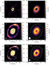 |
Fig. 1 ALMA band 7 continuum observations of HD 100546 from data set A (top), data set B (middle), and from the concatenated set (bottom). The right panels show a zoom into the inner 100 au. The first overlaid contour in the bottom panels corresponds to the 4.5 σ level (0.15 mJy beam−1). |
4.2 Geometrical properties
The geometrical properties of the disk were estimated by fitting continuum emission with GALARIO (Tazzari et al. 2018) and EMCEE (Foreman-Mackey et al. 2013). The underlying model of the brightness profile is the sum of two Gaussian rings. The inclination, position angle, and center of the two rings are free parameters. The GALARIO fit results are reported in the appendix. The best-fit model gives an inclination of 41.7° and a position angle of 146°, in very good agreement with those estimated by Ardila et al. (2007, i = 42° ±5°, PA = 145° ±5°) based on the HST observations. This implies that the inner ring and the outer disk (traced by the HST images) have the same inclination and position angle.
Figure 2 shows the brightness profiles after de-projecting for the disk inclination. The figure shows the azimuthally averaged profile and the projection along the semi-axis (averaged over a range of ± 10°). The inner disk (left panel, from data set A) is asymmetric, as previously noted by Pineda et al. (2019) and Pérez et al. (2020), with a sharp inner edge at around r ~ 20 au and a smoother outer edge extending from nearly 30 au to 50 au. Along the minor axis, the ring is brighter in the northeast direction, peaking at r ~ 31 au. On the contrary, the dust emission along the other semi-axis peaks at r ~ 20–25 au. The outer disk (right panel, from data set A + B) shows multiple features: a narrow ring at r ~ 80 au and an azimuthal asymmetry in the outer ring, with the emission peaking at different radii along the different projections. We note in particular that the emission peaks at r ~ 180 au along the southeastern semimajor axis projection (146°) and at r ~ 220 au along the northwestern semimajor axis (326°). These two peaks correspond to the substructures S1 and S2 in Fig. 1.
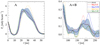 |
Fig. 2 Surface brightness profiles of the inner (left, from data set A) and outer (right, combined data sets A + B) disk of HD 100546. The black curve and the gray region represent the azimuthally averaged profile and standard deviation obtained after de-projecting the images by 42°. The profiles along the semimajor and semiminor axes are overplotted in color; they were obtained by averaging the radial profiles over a range of ±10° around the corresponding axis. |
4.3 Eccentric ring
The azimuthal asymmetries outlined above point to an eccentric outer ring. The left panel of Fig. 3 shows the residual of the band 7 continuum image in polar coordinates after de-projection and subtraction of a Gaussian ring centered at r = 199.5 au with a width of 23.32 au (see the GALARIO fit results in the appendix). Residuals are present, corresponding to S1 and S2. Fitting the position of these residuals with an eccentric ring gives an eccentricity e = 0.07 ±0.01. The right panel of Fig. 3 shows the best-fit eccentric ring overlaid on the surface brightness profile.
4.4 Comparison to near-infrared observations
Figure 4 shows the near-infrared polarimetric observation of HD 100546 taken with SPHERE/IRDIS (the InfraRed Dual-band Imager and Spectrograph) at the VLT (J band Qϕ from Sissa et al. 2018). The main substructures are indicated: the two large-scale spiral arms, two dark lanes, and the disk back side are clearly visible (e.g., Ardila et al. 2007; Boccaletti et al. 2013; Avenhaus et al. 2014; Garufi et al. 2016; Sissa et al. 2018). The ALMA 870 μm continuum emission is overlaid in the bottom panels of Fig. 4: at near-infrared wavelengths, the disk appears radially more extended than at millimeter wavelengths. The inner dark lane is spatially coincident with the ALMA inner ring. This implies that the surface density of themicron-sized particles is partly reduced beyond the inner ring. The near-infrared emission extends inward down to r ~ 11–13 au (see also Avenhaus et al. 2014; Garufi et al. 2016), while the millimeter emission rises beyond 15 au and the emission peak is at r ~ 28 au (as previously noted by Pineda et al. 2014). We note that the ro-vibrational emission of CO (e.g., Brittain et al. 2009; van der Plas et al. 2009; Hein Bertelsen et al. 2014) and OH (e.g., Brittain et al. 2014; Fedele et al. 2015) also extends inward down to r ~ 11–13 au.
4.5 Planet-induced perturbations
The differences in the near-infrared and millimeter surface brightness are likely the outcome of dynamical disk-planet interaction: the large dust grains traced by ALMA are settled to the disk midplane and trapped in two main ring-like structures that are produced by two embedded giant protoplanets; the small dust grains traced by the J band polarimetric observations are dynamically coupled to the gas, which is more extended than the large dust grains both in the vertical and radial direction and diffuses inside the gap (e.g., Zhu et al. 2012). The sharp edge of the inner dust ring at 20 au also implies the presence of a massive inner planet that is needed to stop the inward migration of millimeter dust, as already suggested by several authors (see Sect. 2). The presence of an outer massive planet is consistent with: (1) the outer dust gap, (2) the perturbed dynamics of the gas inward of 100 au (Pineda et al. 2014; Walsh et al. 2017), and (3) the multiple spiral patterns observed in the near-infrared. All of these findings are in agreement with theoretical calculations of disk-planet interactions (e.g., Goldreich & Tremaine 1979; Ogilvie & Lubow 2002; Crida & Morbidelli 2007; Dipierro & Laibe 2017).
Following Rosotti et al. (2016) and Lodato et al. (2019), in the case of a gap opened by a planet, the dust gap width (Δp) scales with the Hill radius of the planet as Δp = ≃5.5RH, where RH depends on the planet (Mp) and stellar (M⋆) masses as ![$[M_{\textrm{p}}/(3M_{\star})]^{1/3}a_{\textrm{p}}$](/articles/aa/full_html/2021/07/aa41278-21/aa41278-21-eq1.png) . The estimated planetary mass is ~ 5.5–6 MJ for a Δp = 100 au and an orbital radius of 100 and 110 au, respectively.
. The estimated planetary mass is ~ 5.5–6 MJ for a Δp = 100 au and an orbital radius of 100 and 110 au, respectively.
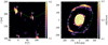 |
Fig. 3 Eccentricity of the outer ring. Left: surface brightness of the outer disk region in polar coordinates after de-projection and subtraction of a Gaussian ring centered at r = 200 au. The dot-dashed green line is the best fit of the outer ring with an eccentricity of 0.07 (see Sect. 4 for details). Right: surface brightness with the eccentric ring overlaid. |
 |
Fig. 4 VLT/SPHERE IRDIS polarimetric observations of HD 100546 (from Sissa et al. 2018) showing the large-scale (left) and small-scale (right) structures. The main substructures are overlaid in the top panels. The ALMA 870 μm contours are overlaid in the bottom panels. |
5 Comparison to hydrodynamical simulations
To answer the question of whether a single massive planet at 100–110 au is capable of producing the structures in the outer disk described above, we carried out a number of 3D smoothed-particle-hydrodynamic (SPH) simulations using the PHANTOM code (Price et al. 2018) and changing the initial conditions in terms of disk mass and size, surface density profile, and planet eccentricity. The following sections present the results of the simulation that qualitatively reproduces the observational findings best.
5.1 Physical setup
To simulate the dynamics and evolution of a disk composed of dust and gas, the multigrain one-fluid method (Hutchison et al. 2018) was adopted. This method is best suited for small values of the Stokes number (St <1). Smoothed-particle-hydrodynamic particles represent both gas and dust and are evolved with an algorithm based on the terminal velocity approximation (Laibe & Price 2014). Back-reaction from the dust onto the gas is naturally included in the code. The system was modeled with a centralstar and two giant planets embedded in the disk, which were allowed to migrate and accrete mass. The fluid self-gravity was neglected.
The diskwas set up as in Toci et al. (2020): The central star was surrounded by a disk of 106 SPH particles, the disk extended from Rin = 5 au to Rout = 300 au, with reference radius R0 = 100 au, and a surface density profile was evaluated according to
![\begin{equation*} \Sigma(R) = \Sigma_0 \left(\frac{ R}{R_0} \right){}^{-p} \exp \left[\left(\frac{R}{R_0} \right){}^{(2-q)} \right]\left(\-\sqrt{\frac{r}{R_{\textrm{in}}}} \right). \end{equation*}](/articles/aa/full_html/2021/07/aa41278-21/aa41278-21-eq2.png) (1)
(1)
The density normalization Σ0 = 1.93 g cm−2 was chosen to set an initial total gas mass of 0.04M⊙ (compatible with the initial disk mass reported by Pinilla et al. 2015b and Miley et al. 2019). The power-law index, p, is equal to 1, while the index q refers only to the sound speed. In the vertical direction, the volume density has a Gaussian profile with a Gaussian width equal to  , where we fixed H∕R = 0.07 at R = R0, and q = 0.25. The gas-to-dust mass ratio was initially set to 100 (hence, the initial dust mass was 4 × 10⁻⁴ M⊙), and gas and dust initially had the same surface density profile. After a few orbits of the planets, the dust settles and forms a layer in the midplane with thickness Hd given by Fromang & Nelson (2009):
  , where Hg is the gas disk height and αSS is the Shakura & Sunyaev (1973) viscosity. Two different dust-sized particles were included to study the behavior of the small and large dust components, a1 = 1.0 μm and a2 = 1.0 mm. The intrinsic grain density was ρd = 1 g cm−2, and the initial dust mass was 0.67 ×10⁻⁴ M⊙ and 3.3 ×10⁻⁴ M⊙ for the small and large dust particles, respectively. With these assumptions, the initial Stokes number (St = ρda1,2∕Σgas) was smaller than 1 throughout the whole disk.
The central star had a mass of 2.4 M⊙; a first giant planet with mass M1,0 = 3 MJ was located inside the inner cavity at a distance of R1,0 = 15 au, and a second planetary mass companion with initial mass M2,0 = 1 MJ was initialized in the outer part of the disk, R2,0 = 170 au, on slightly eccentric orbits with eccentricity e = 0.2. The star and the two planets were represented using sink particles (Bate et al. 1995). The mass accretion radius was set to one-fourth of the Hill radius for the planets and 5 au for the star (as we were not interested in modeling the innermost region of the disk, this assumption does not affect the results of the simulation). The SPH artificial viscosity parameter, αAV, was set to 0.2 in order to have an effective Shakura & Sunyaev (1973) viscosity of αSS= 0.005. The time unit corresponds to the orbital period of the outer planet, Torb = 1880 yr. The simulation was stopped after 50Torb ~ 105 yr. This timescale is large enough to investigate the spiral structures driven by the outer planet (Dong et al. 2016; Rosotti et al. 2019) and the interactions between the planets and the disk.
5.2 SPH results: surface density evolution
The results of the simulations are shown in Fig. 5: the top panels show the surface density distribution of the gas (Σg) and of the large dust grains (Σd, large) at t = 50 Torb. The bottom panels show the time evolution of the azimuthally averaged surface density profiles. The inner planet remains close to its initial position, ai ~15 au, opening a gap in the dust and in the gas with a sharp rim at ~20 au. The outer planet carves a gap in the gas and in the dust while migrating from its initial orbit to a final orbital radius of ao ~ 110 au. The outer planet decreases its migration speed after about 40 Torb; at the end of the simulation (t = 50 Torb), when migration has almost stopped, the gas gap extends from ~80–130 au while the large dust gap is wider (from ~40 au to ~ 150 au) and deeper than the gas one. The interaction between the outer planet and the disk gives rise to a spiral pattern inward and outward of the planetary orbit. The large dust grains are confined in two pressure maxima that are induced by the presence of the two planets: the inner one creates the thick bright inner ring (20–40 au), accumulating all the dust that is drifting from the R < 110 au region, while the outer planet traps all the dust that is drifting from the outermost part of the disk in the second pressure maxima located at ~ 200 au. The presenceof the spiral arms leaves a signature in the dust distribution: Regions of dust over-density are visible wherethe spiral arm crosses the dust rings. At the end of the simulation, the two planets have a mass of M1 = 3.1 MJ and M2 = 8.5 MJ, respectively. We note that the mass of the outer planet is just 1.4 times larger than that estimated in Sect. 4. Figure 6 shows the temporal evolution of the orbital radius and mass of the two planets in the simulation: the mass accretion rate on the inner planet drops after about 10 Torb, and the accretion rate on the outer planet starts to flatten after about 40 Torb; the outer planet mass is about 8.5 MJ at t = 50 Torb. Extrapolating the curve of the mass accretion rate, the final mass of the outer planet is expected to be nearly 10 MJ. During migration, the gas–planet interaction damps the eccentricity of the outer planet, reducing it from 0.2 to 0.05 after 50 orbits. As a consequence, the outer dusty ring is slightly eccentric (e ~ 0.05). Interestingly, in our PHANTOM simulations, when the initial eccentricity of the planet is set to zero (not shown here), the eccentricity of the outer planet grows to 0.05 and 0.1 at t = 50 Torb. The final gas and total dust masses are 2.8 ×10⁻² M⊙ and 4 × 10⁻⁴ M⊙, respectively.
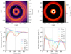 |
Fig. 5 SPH results. Top: surface density of gas and 1 mm dust grains after t = 50 Torb. The positionsof the planets are shown as red dots in the left panel. Bottom: temporal evolution of the azimuthally averaged surface density profiles. The final positions of the two planets are indicated by the vertical dashed lines. The shape of the outer gap, both in gas and in dust, reflect the radial migration of the planet. |
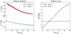 |
Fig. 6 SPH results: temporal evolution of the orbital radius (left) and mass (right) of the two planets. |
5.3 SPH results: synthetic images
Synthetic observations are computed with MCFOST (Pinte et al. 2006, 2009). A Voronoi tessellation maps each SPH particle to an MCFOST cell without interpolation. The DIscANAlysis (DIANA) dust opacity (Woitke et al. 2016) was adopted, assuming a fixed dust mixture composed of 70% silicate and 30% amorphous carbonaceous and a grain size distribution with slope of −3.5 in a range from 0.03 μm to 3 mm. The expected emission maps were computed using ray tracing and 108 photon packets, with a disk inclination of i = 42°, a distance d = 110 pc, and PA = 147°. The stellar spectral model is selected from the stellar isochrones from Siess et al. (2000). Finally, the synthetic 870 μm continuum images were produced with the CASA tasks SYMOBSERVE and SYMANALYZE, adopting the array configuration 4.9 that almost matches the achieved beam of the concatenated data set. Figure 7 shows the synthetic dust continuum images at 870 μm for the 50 Torb snapshot.
The synthetic images reproduce several observational findings, such as the double ring-like structure with the inner ring (~ 20–40 au) much brighter than the outer one (~150–250 au), the wide dust gap (~40–150 au), and the asymmetry in the outer disk. As noted in Sect. 4, there is a tentative detection of a point-like source at nearly 100 aufrom the star (S4). Further observations are needed to confirm the detection and unveil the nature of such emission.
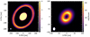 |
Fig. 7 Synthetic ALMA 870 μm continuum images based on the SPH simulations. Left: zoom in on the emission from the inner ring convolved with a beam of 0′′.036 ×0′′.027 matching the angular resolution of data set A. Right: synthetic image convolved with a beam of 0′′.156 ×0′′.127, similar to data set A + B. |
5.4 Simulation caveats
While the synthetic dust continuum images reproduce several of the observational results, the actual flux level of the outer ring is not recovered as it is overestimated by an order of magnitude. This may be due to the assumptions on the physical disk setup and, in particular, to the slope of the surface density profile or to the uncertainties on the radiative transfer parameters, such as the opacity of the dust, its chemical composition, and the boundary values of the grain size distribution; the emission at 870 μm becomes fainter for higher values of amax or for dust composed of silicates only. On the other hand, a larger initial disk size (Rout > 300 au) and a steeper surface density profile (p > 1) could produce a fainter outer disk.
6 Discussion
6.1 Disk-planet interaction
The analysis presented above hints at the presence of two giant protoplanets at ~ 15 au and ~ 110 au. The planets shape the disk structure and dynamics, trapping the large dust grains in two distinct rings: The outer planet traps the dust in a ring-like structure centered at 200 au while the inner planet prevents the inward dust drift, blocking the large grains at r ~ 20–40 au. Dust trapping in multiple rings was proposed by Pinilla et al. (2015b) for the general case of multiple giant protoplanets embedded in a protoplanetary disk and by Pinilla et al. (2015a) in the specific case of HD 100546. A similar configuration has been found in other disks, such as HD 169142, where two giant protoplanets at ~ 18 au and ~ 51 au give rise to a double-ring dust-like structure (e.g., Toci et al. 2020). In the case of HD 100546, the presence of the outer massive planet perturbs the gas structure and dynamics, inducing a two-armed spiral in the R < 100 au part of the disk, similar to the spiral pattern observed in the inner disk region in the near-infrared by, for example, Garufi et al. (2016) and Follette et al. (2017). No substantial misalignment has been found between the inner and outer disk (Sect. 4). The gas spiral arms in the inner disk can also explain the gas dynamics inward of 100 au observed by Pineda et al. (2014, 2019), Walsh et al. (2015). Further ALMA observations of CO isotopologs at medium angular resolution (~ 0′′.15) could potentially reveal the gas spiral structure.
The SPHsimulations presented here suggest that the outer planet may have been formed farther out in the disk (the initial position is 170 au) and may have subsequently migrated inward. Other protoplanetary disks show the imprints of giant protoplanets on wide orbits (R ≳100 au), such as HD 163296 (e.g., Isella et al. 2016, 2018; Pinte et al. 2018), HD 97048 (van der Plas et al. 2017; Pinte et al. 2019), and AS 209 (e.g., Fedele et al. 2018; Guzmán et al. 2018; Favre et al. 2019). The formation of (massive) planets at such a large distance from the star is at odds with the standard core-accretion model and instead favors the gravitational instability scenario (Kratter & Lodato 2016).
6.2 Dust gap and water emission
The presence of the 40–150 au dust gap has some important astrochemical implications regarding the detection of water ice and water vapor from the disk around HD 100546. Honda et al. (2016) reported an absorption feature at 3.1 μm that is likely due to water ice grains. The ice absorption band arises from a region between nearly 40 and 120 au from the star. Far-infrared spectroscopy with the Heterodyne Instrument for the Far-Infrared (HIFI) onboard of Herschel has also revealed emission of the ground-state H2 O lines (Du et al. 2017; van Dishoeck et al. 2021). The velocity profile of the two water lines indicates that the inner radius of the water emission is ~ 40 au, while the outer radius is poorly constrained as the HIFI spectra are spatially unresolved. Both features (ice absorption and gas emission) are in agreement with photo-desorption models (Honda et al. 2016; van Dishoeck et al. 2021). The spatial coincidence between the millimeter dust gap, the water ice absorption, and the ground-state water vapor emission is striking: Because of the lower dust extinction in the dust gap, the stellar UV photons can reach the colder layers and evaporate water molecules via UV photo-desorption. This implies that the dust gap is not fully void of dust, that there must be a residual of small dust grains. This may also explain the recent detection and emission pattern of H2 CO and CH3 OH by Booth et al. (2021).
7 Conclusions
This paper has presented a new analysis of archival ALMA 870 μm images, revealing, in addition to the previously known inner cavity within 20 au, a wide dust gap between r ~ 40–150 au and a previously unresolved faint dust ring beyond 150 au. The emission in the outer disk is not homogeneous, and two main substructures are detected, peaking at ~180 au and ~220 au, respectively. The azimuthally asymmetric emission is likely caused by an eccentric ring with eccentricity e = 0.07 ±0.01. The observationalfindings and the comparison with hydrodynamical simulations hint at the presence of two giant protoplanets at nearly 15 au and 110 au, with masses of ~3.1 MJ and 8.5 MJ, respectively. The massive outer planet challenges current formation models via core accretion.
Acknowledgements
This work was supported by the PRIN-INAF 2019 Planetary Systems At Early Ages (PLATEA). CT and GL have received funding from the European Union’s Horizon 2020 research and innovation programme under the Marie Skłodowska-Curie grant agreement no. 823823 (DUSTBUSTERS RISE project).
Appendix A GALARIO fit results
The geometrical properties of the 870 μm continuum emission were obtained by fitting the visibility of data set B with GALARIO (Tazzari et al. 2018) and EMCEE (Foreman-Mackey et al. 2013) with uniform priors. The brightness profile is the sum of two Gaussian rings with the same inclination, position angle, and phase center:
 (A.1)
(A.1)
The best-fit model parameters are found by minimizing the χ2 :
 (A.2)
(A.2)
where wj is the weight of the observed (uj, vj) visibility points. The posterior distribution is computed as exp(−χ2∕2). EMCEE is initialized with 50 walkers and with 40000 Markov chain Monte Carlo (MCMC) steps. The modeling results are listed Table A.1 along with the initial range of the prior functions. The best-fit values correspond to the 50% percentile of the marginalized distributions, and the uncertainties correspond to half the interval between the 16% and 84% percentiles. The percentiles were computed by reading every ten steps. Figure A.1 shows the 1D and 2D marginalized posterior distributions.
GALARIO modeling results.
 |
Fig. A.1 GALARIO fit results: 1D and 2D marginalized distributions of the posterior sampling obtained with MCMC. |
References
- Acke, B., & van den Ancker, M. E. 2006, A&A, 449, 267 [NASA ADS] [CrossRef] [EDP Sciences] [Google Scholar]
- Andrews, S. M., Wilner, D. J., Zhu, Z., et al. 2016, ApJ, 820, L40 [NASA ADS] [CrossRef] [Google Scholar]
- Ardila, D. R., Golimowski, D. A., Krist, J. E., et al. 2007, ApJ, 665, 512 [NASA ADS] [CrossRef] [Google Scholar]
- Avenhaus, H., Quanz, S. P., Meyer, M. R., et al. 2014, ApJ, 790, 56 [Google Scholar]
- Bate, M. R., Bonnell, I. A., & Price, N. M. 1995, MNRAS, 277, 362 [NASA ADS] [CrossRef] [Google Scholar]
- Booth, A. S., Walsh, C., & Terwisscha van Scheltinga, J. et al. 2021, Nat. Astron., [arXiv:2104.08348] [Google Scholar]
- Boccaletti, A., Pantin, E., Lagrange, A. M., et al. 2013, A&A, 560, A20 [NASA ADS] [CrossRef] [EDP Sciences] [Google Scholar]
- Brittain, S. D., Najita, J. R., & Carr, J. S. 2009, ApJ, 702, 85 [NASA ADS] [CrossRef] [Google Scholar]
- Brittain, S. D., Carr, J. S., Najita, J. R., Quanz, S. P., & Meyer, M. R. 2014, ApJ, 791, 136 [Google Scholar]
- Crida, A., & Morbidelli, A. 2007, MNRAS, 377, 1324 [Google Scholar]
- Currie, T., Cloutier, R., Brittain, S., et al. 2015, ApJ, 814, L27 [Google Scholar]
- Dipierro, G., & Laibe, G. 2017, MNRAS, 469, 1932 [NASA ADS] [CrossRef] [Google Scholar]
- Dong, R., Fung, J., & Chiang, E. 2016, ApJ, 826, 75 [NASA ADS] [CrossRef] [Google Scholar]
- Du, F., Bergin, E. A., Hogerheijde, M., et al. 2017, ApJ, 842, 98 [NASA ADS] [CrossRef] [Google Scholar]
- Favre, C., Fedele, D., Maud, L., et al. 2019, ApJ, 871, 107 [Google Scholar]
- Fedele, D., Bruderer, S., van den Ancker, M. E., & Pascucci, I. 2015, ApJ, 800, 23 [Google Scholar]
- Fedele, D., Carney, M., Hogerheijde, M. R., et al. 2017, A&A, 600, A72 [NASA ADS] [CrossRef] [EDP Sciences] [Google Scholar]
- Fedele, D., Tazzari, M., Booth, R., et al. 2018, A&A, 610, A24 [NASA ADS] [CrossRef] [EDP Sciences] [Google Scholar]
- Follette, K. B., Rameau, J., Dong, R., et al. 2017, AJ, 153, 264 [Google Scholar]
- Foreman-Mackey, D., Hogg, D. W., Lang, D., & Goodman, J. 2013, PASP, 125, 306 [Google Scholar]
- Fromang, S., & Nelson, R. P. 2009, A&A, 496, 597 [NASA ADS] [CrossRef] [EDP Sciences] [Google Scholar]
- Gaia Collaboration (Brown, A. G. A., et al.) 2018, A&A, 616, A1 [NASA ADS] [CrossRef] [EDP Sciences] [Google Scholar]
- Garufi, A., Quanz, S. P., Schmid, H. M., et al. 2016, A&A, 588, A8 [NASA ADS] [CrossRef] [EDP Sciences] [Google Scholar]
- Goldreich, P., & Tremaine, S. 1979, ApJ, 233, 857 [Google Scholar]
- Grady, C. A., Woodgate, B., Heap, S. R., et al. 2005, ApJ, 620, 470 [Google Scholar]
- Guzmán, V. V., Huang, J., Andrews, S. M., et al. 2018, ApJ, 869, L48 [CrossRef] [Google Scholar]
- Hein Bertelsen, R. P., Kamp, I., Goto, M., et al. 2014, A&A, 561, A102 [NASA ADS] [CrossRef] [EDP Sciences] [Google Scholar]
- Honda, M., Kudo, T., Takatsuki, S., et al. 2016, ApJ, 821, 2 [Google Scholar]
- Hutchison, M., Price, D. J., & Laibe, G. 2018, MNRAS, 476, 2186 [NASA ADS] [CrossRef] [Google Scholar]
- Isella, A., Guidi, G., Testi, L., et al. 2016, Phys. Rev. Lett., 117, 251101 [NASA ADS] [CrossRef] [Google Scholar]
- Isella, A., Huang, J., Andrews, S. M., et al. 2018, ApJ, 869, L49 [Google Scholar]
- Keppler, M., Benisty, M., Müller, A., et al. 2018, A&A, 617, A44 [NASA ADS] [CrossRef] [EDP Sciences] [Google Scholar]
- Kratter, K., & Lodato, G. 2016, ARA&A, 54, 271 [Google Scholar]
- Laibe, G., & Price, D. J. 2014, MNRAS, 440, 2136 [NASA ADS] [CrossRef] [Google Scholar]
- Lodato, G., Dipierro, G., Ragusa, E., et al. 2019, MNRAS, 486, 453 [NASA ADS] [CrossRef] [Google Scholar]
- Long, F., Pinilla, P., Herczeg, G. J., et al. 2018, ApJ, 869, 17 [NASA ADS] [CrossRef] [Google Scholar]
- McMullin, J. P., Waters, B., Schiebel, D., Young, W., & Golap, K. 2007, in Astronomical Society of the Pacific Conference Series, 376, Astronomical Data Analysis Software and Systems XVI, eds. R. A. Shaw, F. Hill, & D. J. Bell, 127 [Google Scholar]
- Miley, J. M., Panić, O., Haworth, T. J., et al. 2019, MNRAS, 485, 739 [Google Scholar]
- Nomura, H., Tsukagoshi, T., Kawabe, R., et al. 2016, ApJ, 819, L7 [Google Scholar]
- Ogilvie, G. I., & Lubow, S. H. 2002, MNRAS, 330, 950 [NASA ADS] [CrossRef] [Google Scholar]
- Pérez, S., Casassus, S., Hales, A., et al. 2020, ApJ, 889, L24 [Google Scholar]
- Pineda, J. E., Quanz, S. P., Meru, F., et al. 2014, ApJ, 788, L34 [Google Scholar]
- Pineda, J. E., Szulágyi, J., Quanz, S. P., et al. 2019, ApJ, 871, 48 [Google Scholar]
- Pinilla, P., Birnstiel, T., & Walsh, C. 2015a, A&A, 580, A105 [NASA ADS] [CrossRef] [EDP Sciences] [Google Scholar]
- Pinilla, P., de Juan Ovelar, M., Ataiee, S., et al. 2015b, A&A, 573, A9 [NASA ADS] [CrossRef] [EDP Sciences] [Google Scholar]
- Pinte, C., Ménard, F., Duchêne, G., & Bastien, P. 2006, A&A, 459, 797 [NASA ADS] [CrossRef] [EDP Sciences] [Google Scholar]
- Pinte, C., Harries, T. J., Min, M., et al. 2009, A&A, 498, 967 [NASA ADS] [CrossRef] [EDP Sciences] [Google Scholar]
- Pinte, C., Price, D. J., Ménard, F., et al. 2018, ApJ, 860, L13 [NASA ADS] [CrossRef] [Google Scholar]
- Pinte, C., van der Plas, G., Ménard, F., et al. 2019, Nat. Astron., 3, 1109 [Google Scholar]
- Price, D. J., Wurster, J., Tricco, T. S., et al. 2018, PASA, 35, e031 [Google Scholar]
- Quanz, S. P., Avenhaus, H., Buenzli, E., et al. 2013, ApJ, 766, L2 [NASA ADS] [CrossRef] [Google Scholar]
- Quanz, S. P., Amara, A., Meyer, M. R., et al. 2015, ApJ, 807, 64 [Google Scholar]
- Rosotti, G. P., Juhasz, A., Booth, R. A., & Clarke, C. J. 2016, MNRAS, 459, 2790 [NASA ADS] [CrossRef] [Google Scholar]
- Rosotti, G. P., Booth, R. A., Tazzari, M., et al. 2019, MNRAS, 486, L63 [NASA ADS] [CrossRef] [Google Scholar]
- Shakura, N. I., & Sunyaev, R. A. 1973, A&A, 500, 33 [NASA ADS] [Google Scholar]
- Siess, L., Dufour, E., & Forestini, M. 2000, A&A, 358, 593 [Google Scholar]
- Sissa, E., Gratton, R., Garufi, A., et al. 2018, A&A, 619, A160 [NASA ADS] [CrossRef] [EDP Sciences] [Google Scholar]
- Tazzari, M., Beaujean, F., & Testi, L. 2018, MNRAS, 476, 4527 [Google Scholar]
- Toci, C., Lodato,G., Fedele, D., Testi, L., & Pinte, C. 2020, ApJ, 888, L4 [Google Scholar]
- Ubeira-Gabellini, M. G., Christiaens, V., Lodato, G., et al. 2020, ApJ, 890, L8 [Google Scholar]
- van den Ancker, M. E., de Winter, D., & Tjin A Djie, 1998, A&A, 330, 145 [Google Scholar]
- van der Plas, G., van den Ancker, M. E., Acke, B., et al. 2009, A&A, 500, 1137 [NASA ADS] [CrossRef] [EDP Sciences] [Google Scholar]
- van der Plas, G., Wright, C. M., Ménard, F., et al. 2017, A&A, 597, A32 [NASA ADS] [CrossRef] [EDP Sciences] [Google Scholar]
- van Dishoeck, E. F., Kristensen, L. E., Mottram, J. C., et al. 2021, A&A, 648, A24 [CrossRef] [EDP Sciences] [Google Scholar]
- Vioque, M., Oudmaijer, R. D., Baines, D., Mendigutía, I., & Pérez-Martínez, R. 2018, A&A, 620, A128 [NASA ADS] [CrossRef] [EDP Sciences] [Google Scholar]
- Walsh, C., Juhász, A., Pinilla, P., et al. 2014, ApJ, 791, L6 [Google Scholar]
- Walsh, C., Nomura, H., & van Dishoeck, E. 2015, A&A, 582, A88 [NASA ADS] [CrossRef] [EDP Sciences] [Google Scholar]
- Walsh, C., Juhász, A., Meeus, G., et al. 2016, ApJ, 831, 200 [NASA ADS] [CrossRef] [Google Scholar]
- Walsh, C., Daley, C., Facchini, S., & Juhász, A. 2017, A&A, 607, A114 [NASA ADS] [CrossRef] [EDP Sciences] [Google Scholar]
- Woitke, P., Min, M., Pinte, C., et al. 2016, A&A, 586, A103 [NASA ADS] [CrossRef] [EDP Sciences] [Google Scholar]
- Zhu, Z., Nelson, R. P., Dong, R., Espaillat, C., & Hartmann, L. 2012, ApJ, 755, 6 [NASA ADS] [CrossRef] [Google Scholar]
All Tables
Observation details listing the EBs targeting HD 100546, antenna number, baseline ranges, and source information.
All Figures
|
Fig. 1 ALMA band 7 continuum observations of HD 100546 from data set A (top), data set B (middle), and from the concatenated set (bottom). The right panels show a zoom into the inner 100 au. The first overlaid contour in the bottom panels corresponds to the 4.5 σ level (0.15 mJy beam−1). |
| In the text | |
|
Fig. 2 Surface brightness profiles of the inner (left, from data set A) and outer (right, combined data sets A + B) disk of HD 100546. The black curve and the gray region represent the azimuthally averaged profile and standard deviation obtained after de-projecting the images by 42°. The profiles along the semimajor and semiminor axes are overplotted in color; they were obtained by averaging the radial profiles over a range of ±10° around the corresponding axis. |
| In the text | |
|
Fig. 3 Eccentricity of the outer ring. Left: surface brightness of the outer disk region in polar coordinates after de-projection and subtraction of a Gaussian ring centered at r = 200 au. The dot-dashed green line is the best fit of the outer ring with an eccentricity of 0.07 (see Sect. 4 for details). Right: surface brightness with the eccentric ring overlaid. |
| In the text | |
|
Fig. 4 VLT/SPHERE IRDIS polarimetric observations of HD 100546 (from Sissa et al. 2018) showing the large-scale (left) and small-scale (right) structures. The main substructures are overlaid in the top panels. The ALMA 870 μm contours are overlaid in the bottom panels. |
| In the text | |
|
Fig. 5 SPH results. Top: surface density of gas and 1 mm dust grains after t = 50 Torb. The positionsof the planets are shown as red dots in the left panel. Bottom: temporal evolution of the azimuthally averaged surface density profiles. The final positions of the two planets are indicated by the vertical dashed lines. The shape of the outer gap, both in gas and in dust, reflect the radial migration of the planet. |
| In the text | |
|
Fig. 6 SPH results: temporal evolution of the orbital radius (left) and mass (right) of the two planets. |
| In the text | |
|
Fig. 7 Synthetic ALMA 870 μm continuum images based on the SPH simulations. Left: zoom in on the emission from the inner ring convolved with a beam of 0′′.036 ×0′′.027 matching the angular resolution of data set A. Right: synthetic image convolved with a beam of 0′′.156 ×0′′.127, similar to data set A + B. |
| In the text | |
|
Fig. A.1 GALARIO fit results: 1D and 2D marginalized distributions of the posterior sampling obtained with MCMC. |
| In the text | |
Current usage metrics show cumulative count of Article Views (full-text article views including HTML views, PDF and ePub downloads, according to the available data) and Abstracts Views on Vision4Press platform.
Data correspond to usage on the plateform after 2015. The current usage metrics is available 48-96 hours after online publication and is updated daily on week days.
Initial download of the metrics may take a while.