| Issue |
A&A
Volume 651, July 2021
|
|
|---|---|---|
| Article Number | A112 | |
| Number of page(s) | 16 | |
| Section | The Sun and the Heliosphere | |
| DOI | https://doi.org/10.1051/0004-6361/202140387 | |
| Published online | 30 July 2021 | |
Comparison of active region upflow and core properties using simultaneous spectroscopic observations from IRIS and Hinode
1
PMOD/WRC, Dorfstrasse 33, 7260 Davos Dorf, Switzerland
e-mail: This email address is being protected from spambots. You need JavaScript enabled to view it.
2
ETH-Zurich, Hönggerberg campus, HIT building, Zürich, Switzerland
3
University of Geneva, CUI, 1227 Carouge, Switzerland
4
University of Applied Sciences and Arts Northwestern Switzerland, Bahnhofstrasse 6, 5210 Windisch, Switzerland
5
College of Science, George Mason University, 4400 University Drive, Fairfax, VA 22030, USA
Received:
20
January
2021
Accepted:
7
April
2021
Abstract
Context. The origin of the slow solar wind is still an open issue. It has been suggested that upflows at the edge of active regions are a possible source of the plasma outflow and therefore contribute to the slow solar wind.
Aims. We investigate the origin and morphology of the upflow regions and compare the upflow region and the active region core properties.
Methods. We studied how the plasma properties of flux, Doppler velocity, and non-thermal velocity change throughout the solar atmosphere, from the chromosphere via the transition region to the corona in the upflow region and the core of an active region. We studied limb-to-limb observations of the active region (NOAA 12687) obtained from 14 to 25 November 2017. We analysed spectroscopic data simultaneously obtained from IRIS and Hinode/EIS in the six emission lines Mg II 2796.4Å, C II 1335.71Å, Si IV 1393.76Å, Fe XII 195.12Å, Fe XIII 202.04Å, and Fe XIV 270.52Å and 274.20Å. We studied the mutual relationships between the plasma properties for each emission line, and we compared the plasma properties between the neighbouring formation temperature lines. To find the most characteristic spectra, we classified the spectra in each wavelength using the machine learning technique k-means.
Results. We find that in the upflow region the Doppler velocities of the coronal lines are strongly correlated, but the transition region and coronal lines show no correlation. However, their fluxes are strongly correlated. The upflow region has a lower density and lower temperature than the active region core. In the upflow region, the Doppler velocity and non-thermal velocity show a strong correlation in the coronal lines, but the correlation is not seen in the active region core. At the boundary between the upflow region and the active region core, the upflow region shows an increase in the coronal non-thermal velocity, the emission obtained from the DEM, and the domination of the redshifted regions in the chromosphere.
Conclusions. The obtained results suggest that at least three parallel mechanisms generate the plasma upflow: (1) The reconnection between closed loops and open magnetic field lines in the lower corona or upper chromosphere; (2) the reconnection between the chromospheric small-scale loops and open magnetic field; and (3) the expansion of the magnetic field lines that allows the chromospheric plasma to escape to the solar corona.
Key words: Sun: atmosphere / solar wind / methods: observational / techniques: spectroscopic
© ESO 2021
1. Introduction
The solar atmosphere continuously generates streams of particles known as the solar wind, which creates space weather and the space environment in the Solar System. These particles influence the Earth’s ionosphere and magnetosphere and can have a negative impact on technology and the health of astronauts. The solar wind velocity distribution presents two components of different origins. The source of the fast solar wind (≈800 km s−1 at 1 AU) is well established to be coronal holes, but the origin of the slow solar wind (≈300 km s−1 at 1 AU) is still an open issue. The source of the slow solar wind has been considered to emanate from the coronal hole boundaries (Wang et al. 1990), helmet streamers (Einaudi et al. 1999; Wang et al. 2000), or the edges of the active region (Kojima et al. 1999; Sakao et al. 2007; Harra et al. 2008). In this paper, we focus on the border between the active region and the coronal hole to investigate the origins of the slow solar wind.
Doppler velocity maps, obtained at coronal temperatures, always show a plasma upflow at the edges of active regions (Sakao et al. 2007; Doschek et al. 2007, 2008; Del Zanna 2008; Hara et al. 2008; Harra et al. 2008). The upflow regions have been documented in all observations of active regions regardless of the size, complexity, and stage of evolution. Harra et al. (2017) investigate an upflow region during three solar rotations, but Zangrilli & Poletto (2016) find an upflow region that survived five solar rotations. Plasma upflows have been considered as a source of the solar wind (Sakao et al. 2007; Harra et al. 2008). However, the physical processes that generate the upflow regions are still not confirmed and the following scenarios are considered: plasma circulation in the open coronal magnetic field funnels (Marsch et al. 2008); impulsive heating at the footpoints of active region loops (Harra et al. 2008); chromospheric evaporation due to reconnection driven by flux emergence and braiding by photospheric motions (Del Zanna 2008); chromospheric jets and spicules (De Pontieu et al. 2009, 2017); Alfvén waves triggered by magnetic reconnection (Wang et al. 2015), heating events (Nishizuka & Hara 2011); expansion of large-scale reconnecting loops (Harra et al. 2008), continual active region expansion (Murray et al. 2010); the reconnection between the closed-loop in the active region core and open magnetic field lines create strong pressure imbalances responsible for the plasma upflow (Del Zanna et al. 2011); and the active region magnetic field configuration partially uncovered by the streamers, which allows plasma to easily escape (van Driel-Gesztelyi et al. 2012).
Despite the upflow regions often being co-spatial with open magnetic field lines (Sakao et al. 2007; Harra et al. 2008), not all of these regions are necessarily related to the outflow region and not all of them are the source of the slow solar wind (Edwards et al. 2016). The coronal outflows can originate from the places with a strong gradient of magnetic connectivity, called quasi-separatrix layers (QSLs), where magnetic reconnection transforms the closed magnetic field loops into ‘open’ field or large-scale loops (Baker et al. 2009, 2017). This magnetic field topology allows the coronal upflow material to escape and create the solar wind (Sakao et al. 2007). Moreover, Brooks et al. (2020) show that there are two components of the outflow emission in the active region: a substantial contribution from expanded plasma that appears to have been expelled from closed loops in the active region core, and a contribution from dynamic activity in the active region plage, which has a composition signature that reflects solar photospheric abundances.
Several slow solar wind sources are considered. We present three main scenarios below (Abbo et al. 2016). (1) The expansion model assumes that quasi-static, long-lived, open magnetic field topology allows plasma particles to escape (Wang & Sheeley 1990; Wang 1994). This solar wind speed depends on the flux tube expansion; the faster expansion implies a slower speed. In the active region edges, the expansion of the flux tube is faster than in the coronal hole; thus, the active region edges are a slow solar wind source. (2) Interchange reconnection between the open magnetic field and closed-field lines in the transition region eject particles onto open magnetic field lines creating the solar wind (Fisk & Schwadron 2001). (3) The weak magnetic field of the streamer (pseudo-streamer) cusp allows the material in the underlying closed field lines to escape as a result of the reconnection (Einaudi et al. 1999; Rappazzo et al. 2005).
The origin of the coronal upflow region and its relation to the solar underlying layer of the solar atmosphere is also an open question. One important characteristic of the active region upflows is the blueward asymmetries of coronal line profiles (Harra et al. 2008). Intensive investigations have been performed to understand these asymmetries. The asymmetries also provide important clues regarding the generation mechanisms of the upflows (Tian et al. 2011; McIntosh et al. 2012). However, the mechanisms of the upflow creation and location where these mechanisms occur in the solar atmosphere still remain undiscovered. In this work, we concentrate on the processes responsible for the upflow region creation and evolution. To address this, we study the evolution of the plasma properties from the chromosphere through the transition region to the corona. For plasma diagnostics, we use spectroscopic data obtained simultaneously by the Interface Region Imaging Spectrograph (IRIS; De Pontieu et al. 2014) and Hinode EUV Imaging Spectrometer (Hinode/EIS; Culhane et al. 2007). These observations allow us to analyse the plasma motions (Doppler velocity), and the excess line width above the thermal width, which is known as the non-thermal velocity. Many scenarios have been considered to explain the non-thermal line broadening, such as the propagation of acoustic or magnetohydrodynamics waves (Boland et al. 1975; Coyner & Davila 2011), the small-scale magnetic reconnection events called nanoflares (Parker 1988; Patsourakos & Klimchuk 2006), unresolved laminar flow along with different size loops (Athay & Dere 1991), and the superposition of two or more velocity components along the line of sight (the multiplicity of line-of-sight velocities; Chen et al. 2011; Tian et al. 2011).
Although many papers discuss the dependences between the intensity, Doppler shift, and non-thermal velocity in the upflow region, there is little information on how these parameters and their dependences change with the line formation temperatures from the chromosphere via transition region to the solar corona. Several authors have investigated the temperature dependence of the line parameters, but mainly focus on a narrow temperature range. For instance, Del Zanna (2008), Tripathi et al. (2009), and Warren et al. (2011) performed detailed studies of the Doppler velocities as a function of line formation temperature. For a broader view, we analyse the evolution of the plasma properties in the upflow region in a wide range of temperatures that covers the chromosphere, the transition region, and the corona through the analysis of simultaneous observations obtained by IRIS and Hinode (Sect. 2). We use maps of plasma parameters to study their spatial distribution and the relationships between these plasma parameters (Sects. 3 and 4). Finally, we classify the most characteristic spectra in the active region core and upflow region using an artificial intelligence method to discuss the differences observed (Sect. 5). In Sect. 6, we discuss the relationships between the plasma parameters observed in the different spectral lines and outline the main conclusion and suggestions for further analysis. The methods presented in this work can be used to study the high-resolution spectroscopic data (SPICE; Spice Consortium et al. 2020) from the Solar Orbiter mission (Müller & Marsden 2013; Müller et al. 2020).
2. Data analysis
2.1. Observation
We analysed six datasets of the non-flaring NOAA active region AR12687 obtained from 14 to 25 November 2017. For each observation, we selected a region of interest (ROI) in order to compare the properties of the upflow region and the active region core (Fig. 1, Table 1). We used spectroscopic data obtained simultaneously by IRIS and Hinode/EIS to study the plasma properties. These analyses are carried out for the temperature range from log T/K = 3.8 to log T/K = 6.3 (Table 2). For reliable alignment between the Hinode and IRIS data, we used the images obtained by the Atmospheric Imaging Assembly (SDO/AIA; Lemen et al. 2012). The SDO/AIA data are also used for the differential emission measure (DEM) analysis (Sect. 3.5).
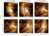 |
Fig. 1. Active region context and regions of interest with upflow and the active region core. All panels show the emission of around 1.5 MK observed in AIA193 Å channel from 14 November 2017 to 25 November 2017. The blue box indicates the Hinode/EIS full FOV. The white dashed and solid boxes highlight the IRIS slit jaw and raster FOV, respectively. The solid white box of panel b is zoomed in Figs. 2 and 3. |
Properties of Hinode/EIS, IRIS, and SDO/AIA observations.
2.2. Hinode EIS
The EIS (Culhane et al. 2007) is a scanning slit spectrometer on board Hinode. The Hinode/EIS observes the upper transition region and the solar corona in two wavebands: 170–210 Å and 250–290 Å with a spectral resolution 0.0223 Å per pixel. The Hinode/EIS can scan the field of view (FOV) up to 9.3 × 8.5 arcmin with the narrowest slit and a spatial scale of 1 arcsec per pixel.
We downloaded the level-0 data from the Hinode/EIS archive1 and focussed on the strong coronal emission lines Fe XII (195.12 Å), Fe XIII (202.04 Å), and Fe XIV (270.52 Å, 274.20 Å). Additionally, we used nine other spectral lines obtained from EIS for the DEM analysis (Table 2, Sect. 3.5). To calibrate Hinode/EIS data, we used a standard routine eis_prep that removed the CCD dark current, cosmic rays pattern, and hot and dusty pixels from the detector exposures. This routine also provided the radiometric calibration from the data number (DN) to the physical unit (erg cm−2 s−1 sr−1 Å−1). Moreover, we applied the correction for a slit tilt and orbital variation of the line position (Warren et al. 2014).
Spectral lines or passbands of Hinode/EIS, IRIS, and SDO/AIA used in our study and analysis.
Using the eis_auto_fit routine2, we fitted a single Gaussian function for Fe XII, Fe XIII, and Fe XIV spectral lines at each spatial pixel. For the Fe XII lines, the χ2 test and the velocity error shows that the single and double Gaussian fits present the same results for our ROIs, hence we chose to use a single Gaussian fit.
The fitted parameters were used to generate the maps of the peak intensity and Doppler velocity. Then, we converted the line-of-sight Doppler velocity to the radial velocity using the direction cosine correction (μ = cos θ). The direction cosine correction is used to reduce the systematic component of the projection effect related to the solar rotation. Using the SolarSoft routine eis_width2velocity, we computed the non-thermal velocity. This routine is based on the equation FWHM2 = (FWHMinstr)2 + 4ln(2)(λ ∖ c)2(Vt + (Vnt)2), where the full width at half maximum (FWHM) FWHMinstr is the instrumental width, λ is the wavelength of the peak of the emission line, c is the speed of light, Vt is the thermal velocity, and Vnt is the non-thermal velocity.
2.3. IRIS
The IRIS (De Pontieu et al. 2014) is a space-based, multi-channel imaging spectrograph that investigates the chromosphere and the transition region. The IRIS instrument provides spectroscopic raster data of the solar atmosphere in the two far-ultraviolet channels (FUV) 1332–1358 Å and 1390–1406 Å and a near-ultraviolet (NUV) channel 2785–2835 Å with a spectral sampling of 12.8 mÅ for FUV and 25.6 mÅ for NUV. The FOV depends on the observation mode and is usually up to 135″ × 175″, but larger raster are possible by re-pointing the satellite.
We analysed level-2 data, downloaded from the IRIS database3. These data were corrected for flat field and geometrical distortion and the dark current was subtracted. The automatic wavelength calibration was confirmed using the O I 1335.60 Å line for FUVS detector, the S I 1401.515 Å for the FUVL detector, and Ni I 2799.474 Å line for the NUV detector. We focussed on several lines of Mg II, C II, and Si IV (Table 2). For all IRIS wavebands analysed in this paper, the raster data were binned to the spatial resolution of the Hinode/EIS, but the spectral resolution was not modified. This binning increased the signal-to-noise ratio.
To obtain the intensity and velocity of the Mg II peaks, we modified the iris_get_mg_features_lev2 routine to work with the spatially binned data and restricted the velocity range to ±40 km s−1. The missing data of intensity and velocity (flagged NaN) were replaced with the interpolated values from the four nearest pixels. For the C II and Si IV spectral lines, we fitted a single Gaussian profile. From the fitted parameters, we created the intensity and Doppler velocity maps. In the last step, the line-of-sight Doppler velocity maps were converted to a radial velocity map using the direction cosine correction μ = cos θ. The χ2 test (IDL XSQ_TEST procedure) was used to test the goodness of fit for the C II and Si IV line for each spatial pixel. We tested the hypothesis that the given observed spectral line intensities are an accurate approximation to the expected Gaussian intensity distribution and assumed hypothesis significance level at 0.05. For further analysis, we used only the fits that fulfilled this hypothesis.
The Slit Jaw Imager (SJI) on board IRIS provides contextual images, showing the area surrounding the slit in four relatively wide bandpasses. The two channels of 55 Å bandpass are centred at 1330 Å and 1400 Å, the other two channels of 4 Å bandpass are centred at 2796 Å and 2832 Å. We used the auxiliary SJI 1400 Å images for data alignment (Sect. 2.5).
2.4. SDO: Atmospheric Imaging Assembly
The AIA (Lemen et al. 2012) provides a continuous monitoring of the full-solar disc in seven EUV and three UV channels that cover the solar atmosphere from the photosphere to the corona. The AIA data are obtained with a spatial scale of 0.6 arcsec per pixel and a temporal resolution of 12 s for EUV channels and 24 s for UV channels.
We used pre-processed SDO data provided by the Joint Science Operations Center (JSOC4). The pre-processing option AIA_SCALE was applied. Therefore, data were corrected for proper plate scaling, shifts, and rotation (i.e. equivalent to level-1.5 data).
To show context and alignment between the Hinode/EIS and IRIS observations, we used the images from SDO/AIA 304 Å, 171 Å, and 193 Å channels (Table 2). Figure 1 shows the context of the active region in AIA 193 Å with the boxes representing the IRIS (white) and Hinode/EIS (blue) FOV. The Hinode/EIS FOV is larger than IRIS FOV, hence our ROI is the latter (solid white box in Fig. 1). The SDO/AIA images of six channels were used for DEM analysis (Sect. 3.5).
2.5. Data alignment
The high-precision alignment of the IRIS and Hinode/EIS data has a direct influence on a comparison of the plasma properties from different layers of the solar atmosphere. Hinode/EIS observes significantly hotter spectral lines than IRIS, and hence for accurate alignment we used both SDO/AIA and IRIS SJI 1400 observations. To keep the same spatial scale of all observations, we interpolated the IRIS and SDO/AIA data to the Hinode/EIS spatial scale. Using a cross-correlation method, we aligned the intensity maps of the lines with close formation temperature. Hence, the maps were aligned according to the following chain: Mg II k2 – Mg II k3 – C II – Si IV -SJI1400 -AIA 304 -AIA 171 -AIA 193 – Fe XII – Fe XIII – Fe XIV. In this chain, the IRIS raster data had a rigid instrumental alignment, similar to the Fe XII and Fe XIII rasters from EIS. The Fe XIV line spectrum is recorded on a different CCD than Fe XII and Fe XIII lines and the offset between these two CCDs of Hinode/EIS is determined using the routine eis_ccd_offset.pro. Finally, IRIS and Hinode data were aligned with the accuracy of the single Hinode/EIS spatial pixel.
3. Results
3.1. Maps of intensity, velocity, and non-thermal velocity
From the six spectroscopic observations presented in Fig. 1 (Table 2), we chose the most representative–the observation obtained on 15 November 2017–to show detailed plots. This observation clearly shows the upflow region and the active region core. The same analysis was carried out for all observations and we present the statistical results for the rest of the observations.
Figures 2 and 3 show the intensity, velocity, and non-thermal velocity maps of the solar corona, transition region and chromosphere observed on 15 November 2017. Based on the Fe XII velocity map (Fig. 2), we defined the upflow region as the blueshifted area with the Doppler velocity lower than −5 km s−1, and the active region core as the redshifted area with the Doppler velocity higher than 5 km s−1.
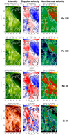 |
Fig. 2. Corona and transition region of the active region core and upflow region observed with Hinode (first three top row) and IRIS (bottom row) on 15 November 2017. The panels show the intensity (left column), Doppler velocity (middle column), and non-thermal velocity (right column). The rows are ordered with decreasing line formation temperatures from 2 MK (Fe XIV line, top row) to 0.08 MK (Si IV, bottom row). To distinguish the active region core and upflow region, we added the contour line of the velocity in Fe XII line of 5 km s−1 and −5 km s−1, respectively. |
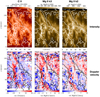 |
Fig. 3. Transition region and chromosphere of the active region core and upflow region observed with IRIS on 15 November 2017. The panels show the intensity (top row) and Doppler velocity (bottom row). The column is ordered with the decreasing line formation temperatures from 40 000 K (C II line, left column) to 6300 K (Mg II k2, right column). To distinguish the active region core and upflow region, we added the contour line of the velocity in Fe XII line of 5 km s−1 and −5 km s−1, respectively (defined in Fig. 2). |
The velocity maps (Fig. 2) obtained from the coronal lines (Fe XII, Fe XIII, and Fe XIV) are similar to each other. These maps show two clear compact features – the blueshifted upflow region and the redshifted active region core. In constrast to the corona, the maps of the underlying layers (Si IV, C II, Mg II) present a huge diversity of Doppler velocities and these maps are rich in numerous small-scale features.
The intensity maps (Figs. 2 and 3) show the bright active region core and a significantly darker upflow region in the coronal lines. In the transition region and chromosphere, the upflow region is only slightly darker than the active region core. The Mg II k2 line shows a chromospheric network pattern (brighter than surroundings) and inter-network regions (darker than surroundings) that in the Mg II k2 velocity map corresponds to red- and blueshifted areas, respectively.
The non-thermal velocities (Fig. 2) were only calculated for optically thin lines observed in the corona (Fe XII, Fe XIII, and Fe XIV) and the transition region (Si IV). In the Fe XIII and Fe XIV lines, the non-thermal velocity is higher in the upflow region than in the active region core. In the Fe XII line, the non-thermal velocity in the whole active region core and one-third of the upflow region is stronger than 30 km s−1. In the rest of the upflow region, the non-thermal velocity is below 30 km s−1. The Fe XIII and Fe XII show stronger non-thermal velocity towards the boundary in the upflow region, suggesting that there is more than one mechanism responsible for a non-thermal spectral line broadening. The non-thermal velocity of Fe XII 195.12 Å is generally higher in the active region core than in the upflow region. In contrast, other corona lines (Fe XIII, Fe XIV) present the stronger average non-thermal velocity in the upflow region than in the active region core. This is very likely because the Fe XII 195.12 Å line is blended with another line at 195.18 Å. It is a density sensitive blend, so the higher density active core implies the stronger line width than in the upflow region where the density is lower. Moreover, the upflow region and the active region core show similar non-thermal velocities in the transition region (Si IV).
3.2. Mutual relation between intensity in closest line
To quantify the relation between the plasma properties of pairs of spectral lines with close formation temperatures (e.g., Fe XII and Fe XIII lines), we used Pearson’s linear correlation coefficient. This coefficient has a value in the range from −1 (negative correlation) to 1 (positive correlation), while 0 defines the lack of correlation. We calculated this correlation coefficient between the intensities of pairs of spectral lines; we calculated close formation temperatures separately for the upflow region (left side of Table 3) and the active region core (right side of Table 3). These analyses showed a strong correlation for all ROIs in all observations.
Linear correlation coefficient between intensities of two close lines for the upflow region and active region core.
In the upflow region, we found strong correlations (left side of Table 3), ranging from 0.57 to 0.99, between intensities from the lines with close formation temperature. In each observation, the relationship between the transition region and coronal lines (Si IV–Fe XII) is slightly weaker than that of other pairs, but the correlation coefficient is at least 0.57.
In the active region core, all pairs of spectral lines show the correlation coefficient around 0.5 or higher, but the correlation is below 0.5 (0.43, 0.49) in only two cases. In general, we can distinguish two groups of the spectral line pairs with the higher correlation coefficient. The coronal pairs present the correlation higher than 0.85. The chromospheric and chromospheric-transition region pairs have correlations higher than 0.71. Similarly to the upflow region, the correlation between the transition region and coronal lines are weaker than in other pairs; the correlation coefficient is below 0.5 in two observations. The nearby limb observation from 24 to 25 November 2017 show a low correlation between Fe XII and Si IV lines (Table 3). This low correlation can be a result of the strong projection effect.
The comparison of the intensity correlations of the pairs of lines with close formation temperature in the upflow region and active region core (Table 3) shows the same trends in both regions, for example two groups of spectral lines with a higher correlation (coronal and chromospheric-transition region) and a weaker correlation between the transition region and coronal line (Si IV–Fe XII). Moreover, we found a higher correlation for the upflow region lines than for the active region core. The high correlation coefficients suggests a clear relation between the structures observed in the close formation temperatures and allows further plasma properties for analysis.
In general, we did not notice a significant relationship between the ROI positions on the solar disc and the correlation coefficient. Still, for large inclination, the projection effects can be important (e.g., observations from 14, 24, and 25 November 2017).
3.3. Relationship between velocities in pairs of lines with close formation temperature
To quantify the dependence between the Doppler velocities in the closest formation temperature lines, we used the same correlation measure as in Sect. 3.2. Table 4 lists the correlation between Doppler velocities for the upflow region (left side) and the active region core (right side).
Linear correlation coefficient between velocities of two close lines for the upflow region and active region core.
In the upflow region, the coronal (Fe XII) and transition region (Si IV) velocities show a very weak correlation. This is because the Si IV is mostly redshifted, whereas the Fe XII is blueshifted. We also found a weak correlation between the Doppler velocities of the C II and Mg II k3 lines.
The pair of the coronal lines (Fe XIII and Fe XII) are well correlated, but the correlation decreases towards higher temperatures (Fe XIV and Fe XIII). We also noticed a strong correlation for the pair of the transition region lines (C II–Si IV) and the pair of the chromospheric lines (Mg II k3 and C II).
The velocities measured present almost the same trends in the active region core and the upflow region. However, the correlation between the coronal (Fe XII) and transition region (Si IV) velocities is stronger in the active region core compared with the upflow region cores.
Table 4 shows that the velocity correlations in the upflow region are stronger nearby the disc centre and weaker towards to limb. We did not notice this effect in the active region core.
3.4. Ratio of the average intensities of downflow to upflow regions.
We calculated the ratio of the average active region core intensity to the upflow region intensity separately for each observation and at each spectral line. Table 5 shows that the intensity ratio increases with the growing line formation temperatures and reaches its highest value in the corona. In the corona, the active region core is always brighter than the upflow region (from 1.5 to 5.6 times), and is usually at least two times brighter than in the transition region and chromosphere. The ratio sharply decreases to around one in the transition region; thus, there the active region core and the upflow region present similar brightnesses. In the chromosphere, the upflow region usually is slightly brighter than the active region core or both regions have similar brightness. Thus, this similarity of intensity in chromosphere can suggest comparable chromospheric heating in the upflow region and the active region core, but further investigations are needed.
Ratio of the average intensities of the active region core to the upflow region.
3.5. Differential emission measure and density diagnostics
The DEM provides information about the plasma distribution in temperature throughout the atmosphere along the line of sight. The DEM is defined as 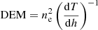 and depends on ne (electron density), T (temperature), and h (height) along the line of sight. We performed a DEM analysis for the observation of 15 November based on SDO/AIA images of 94 Å, 131 Å, 171 Å, 193 Å, and 211 Å, 335 Å channels. We used the regularized DEM inversion method prepared by Hannah & Kontar (2012). To this aim, we chose a set of near-simultaneous images obtained at 14:46:03 UT 15 November 2017. The SDO/AIA images from all the above-mentioned channels were spatially aligned with single SDO/AIA pixel accuracy. In our calculation, we took into account the photon noise and readout noise.
The DEM maps (Fig. 4) show the strongest emission in the upflow region at log T/K = 5.9–6.0 and in the active region core at log T/K = 6.3. This suggests that the upflow region is built from cooler plasma than the active region core. Moreover, the upflow region presents less emission from the transition region temperatures than the active region core (log T/K = 5.6–5.8). The emission distribution suggests that the dominant part of the upflow plasma is generated in the upper transition region or lower corona. In the upflow region, the DEM increases towards the boundary with the active region core.
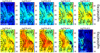 |
Fig. 4. Thermal structure of the upflow region and the active region core for the observation from 15 November. The panels show the DEM map at a temperature range from log T/K = 5.6 to log T/K = 6.5. The FOV is the same as for IRIS raster data (Fig. 2). The contours indicate the ±5 km s−1 plasma flow in the Fe XII line indicating the upflow region and the active region core. |
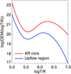 |
Fig. 5. Distribution of differential emission measure for the active region core (red) and upflow region (blue) based on EIS observation of 12 spectral lines from 15 November. The lines show the DEM from the average intensity of the active region core and upflow region as defined in Sect. 3.1 (Fig. 2). |
Additionally, we carried out a DEM analysis based on the observation of 15 November using Hinode/EIS data. We used all available spectral lines as follows: He II (256.312 Å), Fe VIII (185.213), Fe X (184.536 Å, 257.262 Å), Fe XI (180.401 Å), Fe XII (186.880 Å, 193.509 Å, 195.119 Å), Fe XIII (202.044 Å), Fe XIV (274.203 Å), Fe XVI (262.984 Å), and Ca XVII (192.858 Å). The He II line, which is optically thick, is used as a lower-limit constraint on the low temperature part of the DEM, and it is not relevant for the coronal results we focus on. We pre-processed Hinode/EIS data with a standard routine described in Sect. 2. Based on the pre-processed data, the average intensity and their error were computed for the active region core and upflow region for 12 spectral lines, separately. Then, we computed DEM(T) curves for the active region core and upflow region using the CHIANTI method (Del Zanna et al. 2021).
The DEM curves show the strongest emission in the upflow region at log T/K = 6.1 and in the active region core at log T/K = 6.25. Moreover, the upflow region presents less emission than the active region core. Therefore, the DEM analysis of EIS data are consistent with the DEM analysis based on SDO/AIA observation. To clarify, the peak of the DEM for the active region core seems low (log T/K = 6.3). This is because the intensities were averaged over the whole active core region so the contribution from higher temperature loops (log T/K = 6.6; see e.g., Warren et al. 2012) is washed out.
To calculate the average density in the upflow region and active region core, we used the ratio of the Fe XII lines (186.88 Å/195.119 Å) and SSW routine dens_plot5 based on CHIANTI (Del Zanna et al. 2021).
We found a plasma density of 1.05 × 109 cm−3 in the upflow region. In the active region core, the plasma density was 1.38 × 1010 cm−3 (13 times larger than in the upflow region).
4. Non-thermal velocity
We computed non-thermal velocity only for the optically thin lines Si IV, Fe XII, FeXIII, and Fe XIV.
4.1. Relation between Doppler velocity and non-thermal velocity
To analyse the relationship between the Doppler velocity and non-thermal velocity, we prepared a 2D histogram of the probability density function (PDF) of Si IV, Fe XII, Fe XIII, and Fe XIV lines. For the observation of 15 November, the PDF diagrams show a linear relationship between the non-thermal velocity and Doppler velocity for the Fe XII, Fe XIII, Fe XIV lines in the upflow region. We quantified this using Pearson’s linear correlation coefficient. For the active region core, the PDF diagrams show a non-linear correlation for the Si IV line and a lack of correlation for the coronal lines. We used the non-linear Spearman’s rank order correlation between for the active region core (Fig. 6). The analogical analysis was carried out with all observations (Table 6). In the upflow region (Fig. 6 top, Table 6 left side), the PDF diagrams show negative correlation in the coronal temperatures (Fe XII, Fe XIII and Fe XIV) and lack of dependences in the transition region (Si IV). The negative correlation arises from the fact that we chose the upflows to be represented by negative numbers, as compared with the positive numbers and correlation for downflows. The strong negative correlation between the Doppler velocity and non-thermal velocity in the upflow region suggests that the processes responsible for non-thermal line broadening strongly influence upflow in the solar corona. This correlation has been explained as a natural consequence of the superposition of high-speed upflow on the nearly static coronal background (Tian et al. 2011) or the superposition of multiple upflows with slightly shifted velocities (Doschek et al. 2007; Doschek 2012). However, it is also possible that if there is an upflow, more turbulence may be generated on small scales.
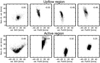 |
Fig. 6. Probability density functions for the non-thermal velocity and Doppler velocity relation for the upflow region (top panels) and the active region core (bottom panels) for the observation from 15 November 2017. For the upflow region panels (top row), the number in the right corner shows the linear correlation coefficient. For the active region core panels (bottom row), the number in the right corner represents a non-linear Spearman’s rank correlation. The panel of the Si IV line in the active region core shows a dichotomy. Thus, we additionally calculated the non-linear correlation coefficient separately for the negative, positive, and absolute Doppler velocity and obtained −0.39, 0.74, and 0.62, respectively. |
Linear correlation coefficient between Doppler and non-thermal velocities for the upflow region and active region core.
In the active region core, we noticed a weak correlation or lack of correlation for Fe XII, Fe XIII, and Fe XIV lines and a positive correlation (of around 0.5) for Si IV lines. Thus, the closed magnetic field-line topology of the active region core reduces the relation between the Doppler velocity and non-thermal velocity, possibly because the plasma motion is restricted within closed magnetic fields. The open magnetic field lines topology of the upflow region allows for more freedom of the ionised plasma motion. Therefore, we suggest that the non-thermal velocity is a result of the multiplicity of the line-of-sight velocities. Moreover, stronger absolute Doppler velocity implies higher non-thermal velocity that can be related for example to increasing turbulence.
4.2. Comparison of the average Doppler and non-thermal velocities in the upflow region and the active region core
We compared the average Doppler and non-thermal velocities computed separately for the upflow region and the active region core. We ordered the average Doppler velocity according to the increasing line formation temperature and represented in Fig. 7a for the upflow region and the active region core. In the solar corona, the upflow region is always blueshifted, and the active region core is redshifted. We found almost the same velocities for the upflow region and the active region core in the transition region and chromosphere. The average Doppler velocities distribution in the upflow region suggests that at least one upflow mechanism is located between Si IV (upper transition region) and Fe XII (lower corona) lines formation temperature. Several previous studies (Teriaca et al. 1999; Peter & Judge 1999; Dadashi et al. 2011) present the distribution of the average Doppler velocity with line formation temperature for active regions, the quiet Sun, or the whole solar disc. However, only few papers focus on the average Doppler velocity distribution in an upflow region (e.g., Del Zanna 2008; Polito et al. 2020).
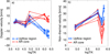 |
Fig. 7. Average Doppler velocities (panel a) and non-thermal velocities (panel b) ordered with the growing line formation temperatures. The panels shows velocities calculated in the upflow region (line blue) and the active region core (red line) for six observations. |
We analysed non-thermal velocities in the same way as the Doppler velocities. These velocities are represented in Fig. 7b and ordered with the growing line formation temperatures (Fig. 7b). In the coronal lines, the non-thermal velocities are higher in the upflow region than in the active region core. Moreover, in the coronal lines the non-thermal velocities show a huge diversity from less than 10 km s−1 in the active region core to almost 40 km s−1 in the upflow region. There is a general resemblance to Doppler velocity; the non-thermal velocity for Fe XIII is usually lower than in Fe XII and Fe XIV lines. In the transition region (Si IV line), the non-thermal velocities are in a range 17–22 km s−1 for the upflow region and active region core. The analysis of the average non-thermal velocity suggests that the magnetic field topology has a strong influence on the non-thermal broadening. In the solar corona, the non-thermal velocity is stronger in the upflow region dominated by the open magnetic field lines compared to the active region core governed by closed corona loops. In general, the relation between the non-thermal velocity and the line formation temperature was investigated in several papers (Chae et al. 1998; Peter 2001; Brooks & Warren 2016). However, we did not find a distribution of the non-thermal velocity with the line formation temperature for an upflow region in previous papers.
5. Spectra classification
We used an unsupervised algorithm known as the k-means clustering algorithm to identify groups of similar spectral profiles (MacQueen 1967). A detailed description of an application on IRIS spectra is available in Panos et al. (2018). The IRIS level-2 raster data were binned to the Hinode spatial scale, but the spectral resolution was not modified. Each spectrum was then normalized by its maximum intensity value before using the k-means algorithm separately on Mg II, C II, and Si IV spectra. The number of groups is often an ill-defined parameter; however, several methods exist that can provide an estimation of this quantity. In this regard, we used the elbow method, which tracks the decrease in variance while incrementally increasing the group number (Thorndike 1953). We obtained eight groups for Mg II, eight groups for CII, and eight groups for SiIV; each group contained spectra with similar shapes.
Figure 8 shows the representative Mg II profiles of the eight groups and the map presents the distribution of the groups in the active region. Group 1–4 (violet-light blue) are characteristics for the upflow region; among these, group 4 (light blue) is the most common. Group 8 (red) is the most representative of the active region. In groups 1–3, the right peaks of Mg II k2 and h2 are stronger than the left peak, which indicates the blueshift, but in the spectra of groups 4, 5, and 8, the left peak is stronger, which indicates redshift (Pereira et al. 2013). Therefore, in the chromosphere of the upflow region we find blueshifted and redshifted areas. Moreover, in the upflow region, the position of group 4 (redshifted) corresponds well to the area with a non-thermal velocity of the Fe XII line stronger than its surroundings (Fig. 2). Therefore, we suggest that group 4 points to a region with the reconnection between active region closed loops and open magnetic field lines of the upflow region, especially that this group is located on the border between the active region core and the upflow region.
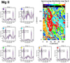 |
Fig. 8. Classification of all Mg II spectra in the FOV into 8 groups using the k-means algorithm. The small panels show the most characteristics spectra classified into 8 groups. The blue line indicates the centroid of k-means, the blue-red line represents the average spectral line profile, and the grey lines show the variance of all profiles in the group. The colour of the rectangle in the spectra corresponds to the colour indicating the location of the spectrum in the distribution map (top right panel). The white contours of the distribution map outline the ±5 km s−1 plasma flow in Fe XII, thus indicating the position of the upflow region and the active region core. |
Comparing groups 4 and 8, we find that the upflow region spectra present a deeper central reversal at the Mg II k3 and Mg II h3 lines centre than the spectra in the active region core. However, further investigations are needed to explain the central reversal difference between the upflow region and active region core.
The maps of the groups of the characteristic spectra distribution for C II and Si IV lines are discussed in more depth in the Appendix A. These maps suggest that the spectra groups of Mg II lines can correspond with the location and shape of the spectra groups of C II lines and Si IV lines. This implies that the structures and physical processes in the chromosphere and transition region are dependent on each other. However, the investigation of other regions are necessary to test the relation between the spectral groups from the different spectral lines.
6. Discussion and conclusions
In this paper, we analysed the plasma properties in the upflow region and the active region core. The plasma properties in the upflow region have been investigated before by many authors (Sect. 1). We extended the analysis to a broader temperature range covering the solar atmosphere from the chromosphere to the corona. We summarize the most important results of our analysis below:
-
The Doppler velocities between adjacent temperature ions in the upflow region show no correlation between the corona and the transition region but a very strong correlation in the corona. The upflow plasma is dominant in the corona.
-
The ratio of intensity of the core to upflow region is high in the upper corona reaching over 5, whereas it is around 1 in the chromosphere. The upflow region has low corona density, but the density is similar between the core and upflow region in the lower atmosphere.
-
The DEM analysis indicates the upflow region has a dominant temperature of log T = 5.9–6.1, whereas the active region core is dominant from log T = 6.2–6.4. The upflow regions are cool, and the emission is strongest closest to the boundary with the active region.
-
The Doppler velocity and non-thermal velocity show a strong correlation in the coronal lines in the upflow region; this correlation is not seen in the active region core. The strength of this relationship may be due to the open field lines in the upflow region.
-
The relationship between both Doppler velocity and non-thermal velocity with temperature has been explored before (e.g., Brooks & Warren 2016). In our case the upflow region deviates in its temperature behaviour above 1 MK.
-
In the upflow region of the chromosphere, there are both red- and blueshifted regions; the redshifted region is more dominant closer to the active region boundary. This is where the strongest non-thermal velocity is seen in the corona.
-
In the upflow region, for each of the investigated spectral lines (Mg II, C II and Si IV) we found several groups of the spectral lines that spatially correspond to each other. Thus, we suggest that more than one process is responsible for the upflow.
Based on the previous papers (Sect. 1) and our results, we suggest three parallel processes that together can generate the plasma upflow (Fig. 9):
-
The interchange reconnection between the open magnetic field lines of the upflow region and closed magnetic field lines (loops) of the active region core in the solar corona.
-
The reconnection between the small-scale loops in the chromosphere and the open magnetic field lines;
-
Expansion of the open magnetic field lines from the photosphere to the corona allows for the plasma upflow due to the waves in the lower solar atmosphere.
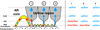 |
Fig. 9. Mechanisms of the plasma upflow formation in the solar atmosphere. The sketch shows the magnetic field topology of the active region core and the upflow region (left side) and the description of the plasma flow in each region that corresponds to the blue (upflow) and red (downflow) arrows on the left side. The active region core is built with the hot coronal loop (yellow). The open magnetic field topology is characteristic for the upflow region (grey). In the chromosphere exists numerous small-scale loops (yellow). The numbers describe the processes responsible for the upflow generation. (1) The reconnection between the closed loop and open magnetic field lines (orange X) in the upper transition region or lower corona. Owing to reconnection, plasma is injected towards the corona and chromosphere. The magnetic field increases towards the chromosphere and can decelerate the plasma flow in this direction. (2) The reconnection between the small-scale chromospheric loop and open magnetic field lines (orange X). Owing to reconnection, plasma is injected towards the lower chromosphere and the transition region. The expanding open magnetic fields lines allow the plasma propagate further to the corona. (3) The open magnetic field structure allows plasma to escape from the chromosphere through the transition region to the solar corona. This process is accelerated by waves propagated in the lower solar atmosphere. |
We review each of these three options and describe in which location and why our observations are consistent with each scenario. Previous papers (e.g., Peter 2001; Tian et al. 2009) present cartoons of the coronal funnels in the quiet Sun or coronal holes. Our sketch (Fig. 9) extends these cartoons for an upflow region considering different upflow scenarios.
6.1. Interchange reconnection between the loops and the open magnetic field lines in the solar corona
In the upflow region, our analysis shows strong blueshift in the corona and redshift in the transition region (Sect. 3.1). This implies no correlation between the coronal and transition region velocities in the upflow region (Sect. 3.3) as noted in the previous studies, for example Warren et al. (2011), and Ugarte-Urra & Warren (2011).
The DEM analysis (Sect. 3.5) indicates the stronger emission closest to the boundary between the upflow region and the active region. This is where the strongest non-thermal velocity is seen in the corona (Sect. 3.1), and the redshifted region dominates in the chromosphere.
We suggest that reconnection occurs between the open magnetic field lines and closed magnetic field loops in the upper transition region or the lower solar corona (Fig. 9, scenario 1). As a result of reconnection, plasma is injected towards the solar corona and photosphere that generates upflow (blueshift) in the corona and downflow (redshift) in the transition region, respectively. The chromospheric redshift can be interpreted as the footprint of the plasma downflow generated during the reconnection. However, the increasing magnetic field concentrations towards the photosphere decelerate this plasma; thus, the plasma velocity of the chromospheric line is closer to 0 km s−1 than in the transition region. The interchange reconnection should be especially efficient close to the border between the active region core and the upflow region where the open and closed magnetic field lines meet each other. As a result of the reconnection, the emission increases, hence the DEM increases too. The turbulence related to reconnection can increase non-thermal line broadening (Gordovskyy et al. 2016).
We received the plasma speed in the upflow region that is significantly lower than the Alfvén speed (Régnier et al. 2008). However, measured reconnection upflow speeds, even during flares, are not at the Alfvén speed either; this is confirmed in various papers, such as Wang et al. (2017). Moreover, the determining of the Alfvén speed is tricky as well (Régnier et al. 2008). Chromospheric evaporation also shows a speed lower than the Alfvén speeds, as presented by Warren (2006), who used a multi-thread model. An explanation for this discrepancy could be that within spectral line broadening multiple blueshift components can exist.
6.2. Reconnection between the small-scale loops and the open magnetic field lines in the chromosphere
The Doppler velocity maps of the transition region lines in the upflow region are dominated by the redshift structures, but these maps also consist in small-scale blueshifted patches (Sect. 3.1). The blueshifted structures in the transition lines of the upflow region were noticed in previous papers (e.g., Del Zanna 2008; He et al. 2010). However, some of the transition region blueshifted patches spatially correspond to the redshifted area in the chromospheric lines. Moreover, our analysis showed a strong correlation of the Doppler velocities of Si IV–C II lines and line, a weaker correlation for C II–Mg II k3 lines, and stronger correlation for Mg II k3–Mg II k2 lines (Sect. 3.3).
We suggest that the reconnection between the chromospheric loops and the open magnetic field lines (Fig. 9, scenario 2) causes the upflow above the reconnection place (above the upper chromosphere) and the downflow below it (middle chromosphere and below).
6.3. Expansion of the open magnetic field lines from the chromosphere to the corona
The Doppler velocity maps show spatially corresponding small-scale blueshifted patches in the chromosphere (Mg II) and transition region (Si IV) of the upflow region. These blueshifted areas are especially visible in the inter-network of Mg II k2 (Sect. 3.1).
We suggest that in the upflow region, the open magnetic field expands from the photosphere to the corona. Therefore, plasma can easily escape from the chromosphere to the corona and further along the open magnetic field lines even when there is no reconnection. The propagation of the waves in the lower solar atmosphere can accelerate the plasma upflow (Fig. 9, scenario 3). Thus, a blueshift observed from the chromosphere via transition region to the solar corona is the most characteristic pattern of the upflow generated by the expanding open flux tubes mechanism.
Polito et al. (2020) find significant differences in spectral signatures below the upflows compared to the core of an active region observed by IRIS. For example, they notice blueshifts in the chromosphere (Mg II, C II) and smaller redshifts and the presence of blueshifts in the transition region (Si IV) below the coronal upflows (Fe XII). This connection between the chromosphere, transition region, and corona suggests that the expanding magnetic field scenario can allow jets and spicules to create the upflow.
6.4. Comparison of the upflow region and the active region core
The spectral profile shape classification (Sect. 5) shows a clear difference between the upflow region and the active region core in the chromosphere (Mg II, C II) and transition region (Si IV). We distinguished several groups of the Mg II profiles. Profiles within the same group are similar, but profiles from different groups consist of significantly different spectra. We noticed the stronger central reversal of Mg II k3 and Mg II h3 in the upflow region than in the active region core. To understand the Mg II line properties and also explain the deep central reversal differences between the upflow region and the active region core, we require additional observations and simulations.
The ratio of the intensity of the core to upflow region (Sect. 3.4) shows that the coronal plasma density is lower in the upflow region than in the active region core. Moreover, the DEM analysis (Sect. 3.5) indicates that the coronal plasma is cooler in the upflow region than in the active region core. The open magnetic field structures dominate the upflow region. But the active region core is rich in the coronal loops, that is closed magnetic field structures preventing the plasma from escaping. Therefore, in the upflow region the plasma can escape more readily into space, hence, the density and temperature of the coronal plasma in the upflow region are lower than in the active region core. However, in the chromosphere and the transition region, the feeds of the different coronal structures look the same (Peter 2001), hence the average intensity of the active region core and upflow region are similar.
The Doppler and non-thermal velocity change with the growing line formation temperature (Sect. 4.2). The increase in the negative Doppler velocity in the upflow region with temperature is due to the plasma acceleration in the open magnetic field lines. Considering the two-component (Tian et al. 2011) or three-component scenarios (McIntosh et al. 2012), there is an alternative interpretation of this observational result: the different relative contributions of the fast upflow component and the cooling downflow component at different temperatures (Wang et al. 2013). The deviation of the non-thermal velocity in the temperature above 1 MK suggests that different mechanisms can be responsible for the non-thermal heating in the upflow region and the active region core.
The strong correlation between the Doppler and non-thermal velocity (Sect. 4.1) observed in the coronal line of the upflow region and a lack of this correlation in the active region core suggest that the magnetic field topology can have a significant influence on the non-thermal heating mechanism. It is also possible that in these two regions, there are different non-thermal heating mechanisms at work. However, it is difficult to point out which non-thermal heating mechanism plays a dominant role in our ROIs. Thus, further investigation of non-thermal velocity is necessary.
Acknowledgments
This work is supported by Swiss National Science Foundation – SNF. The work of DHB was performed under contract to the Naval Research Laboratory and was funded by the NASA Hinode program. SDO data are courtesy of NASA/SDO and the AIA, EVE, and HMI science teams. IRIS is a NASA small explorer mission developed and operated by LMSAL with mission operations executed at NASA Ames Research Center and major contributions to downlink communications funded by ESA and the Norwegian Space Centre. Hinode is a Japanese mission developed and launched by ISAS/JAXA, with NAOJ as domestic partner and NASA and STFC (UK) as international partners. It is operated by these agencies in co-operation with ESA and NSC (Norway).
References
- Abbo, L., Ofman, L., Antiochos, S. K., et al. 2016, Space Sci. Rev., 201, 55 [NASA ADS] [CrossRef] [Google Scholar]
- Athay, R. G., & Dere, K. P. 1991, ApJ, 381, 323 [CrossRef] [Google Scholar]
- Baker, D., van Driel-Gesztelyi, L., Mandrini, C. H., Démoulin, P., & Murray, M. J. 2009, ApJ, 705, 926 [CrossRef] [Google Scholar]
- Baker, D., Janvier, M., Démoulin, P., & Mandrini, C. H., 2017, Sol. Phys., 292, 46 [CrossRef] [Google Scholar]
- Boland, B. C., Dyer, E. P., Firth, J. G., et al. 1975, MNRAS, 171, 697 [NASA ADS] [CrossRef] [Google Scholar]
- Brooks, D. H., & Warren, H. P. 2016, ApJ, 820, 63 [Google Scholar]
- Brooks, D. H., Winebarger, A. R., Savage, S., et al. 2020, ApJ, 894, 144 [Google Scholar]
- Chae, J., Schühle, U., & Lemaire, P. 1998, ApJ, 505, 957 [CrossRef] [Google Scholar]
- Chen, F., Ding, M. D., Chen, P. F., & Harra, L. K. 2011, ApJ, 740, 116 [NASA ADS] [CrossRef] [Google Scholar]
- Coyner, A. J., & Davila, J. M. 2011, ApJ, 742, 115 [CrossRef] [Google Scholar]
- Culhane, J. L., Harra, L. K., James, A. M., et al. 2007, Sol. Phys., 243, 19 [Google Scholar]
- Dadashi, N., Teriaca, L., & Solanki, S. K. 2011, A&A, 534, A90 [NASA ADS] [CrossRef] [EDP Sciences] [Google Scholar]
- De Pontieu, B., McIntosh, S. W., Hansteen, V. H., & Schrijver, C. J. 2009, ApJ, 701, L1 [NASA ADS] [CrossRef] [Google Scholar]
- De Pontieu, B., Title, A. M., Lemen, J. R., et al. 2014, Sol. Phys., 289, 2733 [NASA ADS] [CrossRef] [Google Scholar]
- De Pontieu, B., De Moortel, I., Martinez-Sykora, J., & McIntosh, S. W. 2017, ApJ, 845, L18 [NASA ADS] [CrossRef] [Google Scholar]
- Del Zanna, G. 2008, A&A, 481, L49 [NASA ADS] [CrossRef] [EDP Sciences] [Google Scholar]
- Del Zanna, G., Aulanier, G., Klein, K. L., & Török, T. 2011, A&A, 526, A137 [NASA ADS] [CrossRef] [EDP Sciences] [Google Scholar]
- Del Zanna, G., Dere, K. P., Young, P. R., & Landi, E. 2021, ApJ, 909, 38 [CrossRef] [Google Scholar]
- Doschek, G. A. 2012, ApJ, 754, 153 [NASA ADS] [CrossRef] [Google Scholar]
- Doschek, G. A., Mariska, J. T., Warren, H. P., et al. 2007, ApJ, 667, L109 [NASA ADS] [CrossRef] [Google Scholar]
- Doschek, G. A., Warren, H. P., Mariska, J. T., et al. 2008, ApJ, 686, 1362 [NASA ADS] [CrossRef] [Google Scholar]
- Edwards, S. J., Parnell, C. E., Harra, L. K., Culhane, J. L., & Brooks, D. H. 2016, Sol. Phys., 291, 117 [Google Scholar]
- Einaudi, G., Boncinelli, P., Dahlburg, R. B., & Karpen, J. T. 1999, J. Geophys. Res., 104, 521 [NASA ADS] [CrossRef] [Google Scholar]
- Fisk, L. A., & Schwadron, N. A. 2001, Space Sci. Rev., 97, 21 [CrossRef] [Google Scholar]
- Gordovskyy, M., Kontar, E. P., & Browning, P. K. 2016, A&A, 589, A104 [NASA ADS] [CrossRef] [EDP Sciences] [Google Scholar]
- Hannah, I. G., & Kontar, E. P. 2012, A&A, 539, A146 [NASA ADS] [CrossRef] [EDP Sciences] [Google Scholar]
- Hara, H., Watanabe, T., Harra, L. K., et al. 2008, ApJ, 678, L67 [NASA ADS] [CrossRef] [Google Scholar]
- Harra, L. K., Sakao, T., Mandrini, C. H., et al. 2008, ApJ, 676, L147 [Google Scholar]
- Harra, L. K., Ugarte-Urra, I., De Rosa, M., et al. 2017, PASJ, 69, 47 [NASA ADS] [CrossRef] [Google Scholar]
- He, J. S., Marsch, E., Tu, C. Y., Guo, L. J., & Tian, H. 2010, A&A, 516, A14 [NASA ADS] [CrossRef] [EDP Sciences] [Google Scholar]
- Kojima, M., Fujiki, K., Ohmi, T., et al. 1999, J. Geophys. Res., 104, 16993 [NASA ADS] [CrossRef] [Google Scholar]
- Lemen, J. R., Title, A. M., Akin, D. J., et al. 2012, Sol. Phys., 275, 17 [Google Scholar]
- MacQueen, J. 1967, in Proceedings of the Fifth Berkeley Symposium on Mathematical Statistics and Probability, Volume 1: Statistics (Berkeley, Calif.: University of California Press), 281 [Google Scholar]
- Marsch, E., Tian, H., Sun, J., Curdt, W., & Wiegelmann, T. 2008, ApJ, 685, 1262 [NASA ADS] [CrossRef] [Google Scholar]
- McIntosh, S. W., Tian, H., Sechler, M., & De Pontieu, B. 2012, ApJ, 749, 60 [NASA ADS] [CrossRef] [Google Scholar]
- Müller, D., Marsden, R. G., & St Cyr, O. C., & Gilbert, H. R., 2013, Sol. Phys., 285, 25 [Google Scholar]
- Müller, D., St. Cyr, O. C., Zouganelis, I., et al. 2020, A&A, 642, A1 [CrossRef] [EDP Sciences] [Google Scholar]
- Murray, M. J., Baker, D., van Driel-Gesztelyi, L., & Sun, J. 2010, Sol. Phys., 261, 253 [NASA ADS] [CrossRef] [Google Scholar]
- Nishizuka, N., & Hara, H. 2011, ApJ, 737, L43 [NASA ADS] [CrossRef] [Google Scholar]
- Panos, B., Kleint, L., Huwyler, C., et al. 2018, ApJ, 861, 62 [Google Scholar]
- Parker, E. N. 1988, ApJ, 330, 474 [Google Scholar]
- Patsourakos, S., & Klimchuk, J. A. 2006, ApJ, 647, 1452 [NASA ADS] [CrossRef] [Google Scholar]
- Pereira, T. M. D., Leenaarts, J., De Pontieu, B., Carlsson, M., & Uitenbroek, H. 2013, ApJ, 778, 143 [NASA ADS] [CrossRef] [Google Scholar]
- Peter, H. 2001, A&A, 374, 1108 [NASA ADS] [CrossRef] [EDP Sciences] [Google Scholar]
- Peter, H., & Judge, P. G. 1999, ApJ, 522, 1148 [NASA ADS] [CrossRef] [Google Scholar]
- Polito, V., De Pontieu, B., Testa, P., Brooks, D. H., & Hansteen, V. 2020, ApJ, 903, 68 [CrossRef] [Google Scholar]
- Rappazzo, A. F., Velli, M., Einaudi, G., & Dahlburg, R. B. 2005, ApJ, 633, 474 [NASA ADS] [CrossRef] [Google Scholar]
- Régnier, S., Priest, E. R., & Hood, A. W. 2008, A&A, 491, 297 [NASA ADS] [CrossRef] [EDP Sciences] [Google Scholar]
- Sakao, T., Kano, R., Narukage, N., et al. 2007, Science, 318, 1585 [NASA ADS] [CrossRef] [PubMed] [Google Scholar]
- Spice Consortium, Anderson, M., Appourchaux, T., et al. 2020, A&A, 642, A14 [CrossRef] [EDP Sciences] [Google Scholar]
- Teriaca, L., Banerjee, D., & Doyle, J. G. 1999, A&A, 349, 636 [NASA ADS] [Google Scholar]
- Thorndike, R. L. 1953, Psychometrika, 18, 62 [CrossRef] [Google Scholar]
- Tian, H., Marsch, E., Curdt, W., & He, J. 2009, ApJ, 704, 883 [NASA ADS] [CrossRef] [Google Scholar]
- Tian, H., McIntosh, S. W., De Pontieu, B., et al. 2011, ApJ, 738, 18 [NASA ADS] [CrossRef] [Google Scholar]
- Tripathi, D., Mason, H. E., Dwivedi, B. N., del Zanna, G., & Young, P. R. 2009, ApJ, 694, 1256 [NASA ADS] [CrossRef] [Google Scholar]
- Ugarte-Urra, I., & Warren, H. P. 2011, ApJ, 730, 37 [NASA ADS] [CrossRef] [Google Scholar]
- van Driel-Gesztelyi, L., Culhane, J. L., Baker, D., et al. 2012, Sol. Phys., 281, 237 [Google Scholar]
- Wang, Y. M. 1994, ApJ, 437, L67 [Google Scholar]
- Wang, Y. M., & Sheeley, N. R., Jr. 1990, ApJ, 355, 726 [Google Scholar]
- Wang, Y. M., Sheeley, N. R., Jr., & Nash, A. G. 1990, Nature, 347, 439 [NASA ADS] [CrossRef] [Google Scholar]
- Wang, Y. M., Sheeley, N. R., Socker, D. G., Howard, R. A., & Rich, N. B. 2000, J. Geophys. Res., 105, 25133 [NASA ADS] [CrossRef] [Google Scholar]
- Wang, X., McIntosh, S. W., Curdt, W., et al. 2013, A&A, 557, A126 [NASA ADS] [CrossRef] [EDP Sciences] [Google Scholar]
- Wang, L. C., Li, L. J., Ma, Z. W., Zhang, X., & Lee, L. C. 2015, Phys. Lett. A, 379, 2068 [CrossRef] [Google Scholar]
- Wang, J., Simões, P. J. A., Jeffrey, N. L. S., et al. 2017, ApJ, 847, L1 [NASA ADS] [CrossRef] [Google Scholar]
- Warren, H. P. 2006, ApJ, 637, 522 [NASA ADS] [CrossRef] [Google Scholar]
- Warren, H. P., Ugarte-Urra, I., Young, P. R., & Stenborg, G. 2011, ApJ, 727, 58 [NASA ADS] [CrossRef] [Google Scholar]
- Warren, H. P., Winebarger, A. R., & Brooks, D. H. 2012, ApJ, 759, 141 [NASA ADS] [CrossRef] [Google Scholar]
- Warren, H. P., Ugarte-Urra, I., & Landi, E. 2014, ApJS, 213, 11 [NASA ADS] [CrossRef] [Google Scholar]
- Zangrilli, L., & Poletto, G. 2016, A&A, 594, A40 [CrossRef] [EDP Sciences] [Google Scholar]
Appendix A: Spectra classification
We used the k-means method to classify the groups of similar spectral lines in an analogous way as in Sect. 2. Figure A.1 shows the representative spectra and their distribution map for Si IV (a) and C II (b) lines. These maps show that the upflow region group of spectral lines in Fig. 8 (group 4, light blue) clearly corresponds to groups 3 and 4 (blue) in Si IV (Fig. A.1a) and groups 4 (blue) and 5 (green) in C II (Fig. A.1b). The relationship between the active region core groups is even stronger, group 8 (red) in Fig. 8 corresponds to Si IV group 8 (red) in Fig. A.1a and C II group 8 (red) in Fig. A.1b.
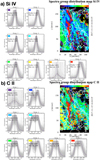 |
Fig. A.1. Groups of the most characteristics spectra of Si IV(a) and C II (b). The small panels show the most characteristics spectra in 8 groups for Si IV (a) and 8 groups of C II (b). The blue line indicates the most characteristic profile (the centroid of k-means), the blue-red line indicates the average spectral line profile, and the grey line represents all profiles in the group. The colour of the rectangular box (right top of the spectra panel) indicates the location of the spectrum in the distribution map (top right panel). The white contours of the distribution map represent the ±5 km s−1 plasma flow in Fe XII, thus indicating the position of the upflow region and the active region core. |
All Tables
Spectral lines or passbands of Hinode/EIS, IRIS, and SDO/AIA used in our study and analysis.
Linear correlation coefficient between intensities of two close lines for the upflow region and active region core.
Linear correlation coefficient between velocities of two close lines for the upflow region and active region core.
Ratio of the average intensities of the active region core to the upflow region.
Linear correlation coefficient between Doppler and non-thermal velocities for the upflow region and active region core.
All Figures
|
Fig. 1. Active region context and regions of interest with upflow and the active region core. All panels show the emission of around 1.5 MK observed in AIA193 Å channel from 14 November 2017 to 25 November 2017. The blue box indicates the Hinode/EIS full FOV. The white dashed and solid boxes highlight the IRIS slit jaw and raster FOV, respectively. The solid white box of panel b is zoomed in Figs. 2 and 3. |
| In the text | |
|
Fig. 2. Corona and transition region of the active region core and upflow region observed with Hinode (first three top row) and IRIS (bottom row) on 15 November 2017. The panels show the intensity (left column), Doppler velocity (middle column), and non-thermal velocity (right column). The rows are ordered with decreasing line formation temperatures from 2 MK (Fe XIV line, top row) to 0.08 MK (Si IV, bottom row). To distinguish the active region core and upflow region, we added the contour line of the velocity in Fe XII line of 5 km s−1 and −5 km s−1, respectively. |
| In the text | |
|
Fig. 3. Transition region and chromosphere of the active region core and upflow region observed with IRIS on 15 November 2017. The panels show the intensity (top row) and Doppler velocity (bottom row). The column is ordered with the decreasing line formation temperatures from 40 000 K (C II line, left column) to 6300 K (Mg II k2, right column). To distinguish the active region core and upflow region, we added the contour line of the velocity in Fe XII line of 5 km s−1 and −5 km s−1, respectively (defined in Fig. 2). |
| In the text | |
|
Fig. 4. Thermal structure of the upflow region and the active region core for the observation from 15 November. The panels show the DEM map at a temperature range from log T/K = 5.6 to log T/K = 6.5. The FOV is the same as for IRIS raster data (Fig. 2). The contours indicate the ±5 km s−1 plasma flow in the Fe XII line indicating the upflow region and the active region core. |
| In the text | |
|
Fig. 5. Distribution of differential emission measure for the active region core (red) and upflow region (blue) based on EIS observation of 12 spectral lines from 15 November. The lines show the DEM from the average intensity of the active region core and upflow region as defined in Sect. 3.1 (Fig. 2). |
| In the text | |
|
Fig. 6. Probability density functions for the non-thermal velocity and Doppler velocity relation for the upflow region (top panels) and the active region core (bottom panels) for the observation from 15 November 2017. For the upflow region panels (top row), the number in the right corner shows the linear correlation coefficient. For the active region core panels (bottom row), the number in the right corner represents a non-linear Spearman’s rank correlation. The panel of the Si IV line in the active region core shows a dichotomy. Thus, we additionally calculated the non-linear correlation coefficient separately for the negative, positive, and absolute Doppler velocity and obtained −0.39, 0.74, and 0.62, respectively. |
| In the text | |
|
Fig. 7. Average Doppler velocities (panel a) and non-thermal velocities (panel b) ordered with the growing line formation temperatures. The panels shows velocities calculated in the upflow region (line blue) and the active region core (red line) for six observations. |
| In the text | |
|
Fig. 8. Classification of all Mg II spectra in the FOV into 8 groups using the k-means algorithm. The small panels show the most characteristics spectra classified into 8 groups. The blue line indicates the centroid of k-means, the blue-red line represents the average spectral line profile, and the grey lines show the variance of all profiles in the group. The colour of the rectangle in the spectra corresponds to the colour indicating the location of the spectrum in the distribution map (top right panel). The white contours of the distribution map outline the ±5 km s−1 plasma flow in Fe XII, thus indicating the position of the upflow region and the active region core. |
| In the text | |
|
Fig. 9. Mechanisms of the plasma upflow formation in the solar atmosphere. The sketch shows the magnetic field topology of the active region core and the upflow region (left side) and the description of the plasma flow in each region that corresponds to the blue (upflow) and red (downflow) arrows on the left side. The active region core is built with the hot coronal loop (yellow). The open magnetic field topology is characteristic for the upflow region (grey). In the chromosphere exists numerous small-scale loops (yellow). The numbers describe the processes responsible for the upflow generation. (1) The reconnection between the closed loop and open magnetic field lines (orange X) in the upper transition region or lower corona. Owing to reconnection, plasma is injected towards the corona and chromosphere. The magnetic field increases towards the chromosphere and can decelerate the plasma flow in this direction. (2) The reconnection between the small-scale chromospheric loop and open magnetic field lines (orange X). Owing to reconnection, plasma is injected towards the lower chromosphere and the transition region. The expanding open magnetic fields lines allow the plasma propagate further to the corona. (3) The open magnetic field structure allows plasma to escape from the chromosphere through the transition region to the solar corona. This process is accelerated by waves propagated in the lower solar atmosphere. |
| In the text | |
|
Fig. A.1. Groups of the most characteristics spectra of Si IV(a) and C II (b). The small panels show the most characteristics spectra in 8 groups for Si IV (a) and 8 groups of C II (b). The blue line indicates the most characteristic profile (the centroid of k-means), the blue-red line indicates the average spectral line profile, and the grey line represents all profiles in the group. The colour of the rectangular box (right top of the spectra panel) indicates the location of the spectrum in the distribution map (top right panel). The white contours of the distribution map represent the ±5 km s−1 plasma flow in Fe XII, thus indicating the position of the upflow region and the active region core. |
| In the text | |
Current usage metrics show cumulative count of Article Views (full-text article views including HTML views, PDF and ePub downloads, according to the available data) and Abstracts Views on Vision4Press platform.
Data correspond to usage on the plateform after 2015. The current usage metrics is available 48-96 hours after online publication and is updated daily on week days.
Initial download of the metrics may take a while.