| Issue |
A&A
Volume 651, July 2021
|
|
|---|---|---|
| Article Number | A74 | |
| Number of page(s) | 19 | |
| Section | Extragalactic astronomy | |
| DOI | https://doi.org/10.1051/0004-6361/202040198 | |
| Published online | 16 July 2021 | |
Interferometric monitoring of gamma-ray bright AGNs: Measuring the magnetic field strength of 4C +29.45⋆
1
Korea Astronomy and Space Science Institute, 776 Daedeok-daero, Yuseong-gu, Daejeon 34055, Korea
e-mail: This email address is being protected from spambots. You need JavaScript enabled to view it.
2
University of Science and Technology, Korea, 217 Gajeong-ro, Yuseong-gu, Daejeon 34113, Korea
3
Department of Physics and Astronomy, Sejong University, 209 Neungdong-ro, Gwangjin-gu, Seoul, South Korea
4
Department of Physics, Faculty of Science, University of Malaya, 50603 Kuala Lumpur, Malaysia
5
Max-Planck-Institut für Radioastronomie, Auf dem Hügel 69, 53121 Bonn, Germany
6
Institute of Astronomy and Astrophysics, Academia Sinica, 11F of Astronomy-Mathematics Building, AS/NTU No. 1, Sec. 4, Roosevelt Rd, Taipei 10617, Taiwan, R.O.C.
7
National Astronomical Observatory of Japan, 2-21-1 Osawa, Mitaka, Tokyo 181-8588, Japan
8
Kogakuin University of Technology & Engineering, Academic Support Center, 2665-1 Nakano, Hachioji, Tokyo 192-0015, Japan
9
Department of Physics and Astronomy, Seoul National University, Gwanak-gu, Seoul 08826, Korea
10
SNU Astronomy Research Center, Seoul National University, Gwanak-gu, Seoul 08826, Korea
Received:
22
December
2020
Accepted:
30
April
2021
Abstract
Aims. We present the results of multi-epoch, multifrequency monitoring of blazar 4C +29.45, which was regularly monitored as part of the Interferometric Monitoring of GAmma-ray Bright Active Galactic Nuclei (iMOGABA) program – a key science program of the Korean Very long baseline interferometry Network (KVN).
Methods. Observations were conducted simultaneously at 22, 43, 86, and 129 GHz over the 4 years from 5 December 2012 to 28 December 2016. We also used additional data from the 15 GHz Owens Valley Radio Observatory (OVRO) monitoring program.
Results. From the 15 GHz light curve, we estimated the variability timescales of the source during several radio flux enhancements. We found that the source experienced six radio flux enhancements with variability timescales of 9–187 days during the observing period, yielding corresponding variability Doppler factors of 9–27. From the simultaneous multifrequency KVN observations, we were able to obtain accurate radio spectra of the source and hence to more precisely measure the turnover frequencies νr, of synchrotron self-absorption (SSA) emission with a mean value of νr̅ = 28.9 GHz. Using jet geometry assumptions, we estimated the size of the emitting region at the turnover frequency. We found that the equipartition magnetic field strength is up to two orders of magnitude higher than the SSA magnetic field strength (0.001–0.1 G). This is consistent with the source being particle dominated. We performed a careful analysis of the systematic errors related to the making of these estimations.
Conclusions. From the results, we concluded that the equipartition region is located upstream from the SSA region.
Key words: galaxies: active / galaxies: jets / BL Lacertae objects: individual: J1159+2914
Lightcurves are only available at the CDS via anonymous ftp to cdsarc.u-strasbg.fr (130.79.128.5) or via http://cdsarc.u-strasbg.fr/viz-bin/cat/J/A+A/651/A74
EACOA fellow.
© ESO 2021
1. Introduction
Blazars are a category of active galactic nuclei (AGNs) where the relativistic jet is oriented almost directly toward us (Angel & Stockman 1980). Because of the small viewing angle (e.g., ≤5 degrees; Jorstad et al. 2017), the emission from most blazars shows dynamic variations in total flux density and polarization, and many of these blazars are highly Doppler boosted (Madau et al. 1987). Very long baseline interferometry (VLBI) studies of relativistic jets have revealed that the jets are highly collimated and exhibit acceleration (Jorstad et al. 2017; Homan et al. 2015). Many studies have tried to explain how the jets can be accelerated and collimated (e.g., Homan et al. 2015; Nakamura & Asada 2013). One potential scenario is that the magnetic fields around the jet accelerate and collimate the jet (Begelman et al. 1984; Komissarov et al. 2007). Meanwhile, shocks in jets make the magnetic fields aligned or tangled (Marscher et al. 2008). Therefore, it is important to study the magnetic field properties around blazar jets. As a well-known example for such studies, M87, one of the brightest and closest AGNs, has been widely studied, including its magnetic field properties (Asada & Nakamura 2012; Asada et al. 2014; Hada et al. 2016; Kim et al. 2018c; Mertens et al. 2016; Nakamura et al. 2018; EHTC 2019; Park et al. 2019a,b).
One way to study magnetic fields is to measure the polarization of the emission. When relativistic electrons pass through magnetic fields, these electrons emit synchrotron radiations that can be linearly polarized by up to 70% (Hales et al. 2017). Many studies have performed VLBI polarization observations of jets in order to reveal the structure of the magnetic fields (e.g., Gabuzda 2017). Agudo et al. (2018) found that the magnetic fields measured at shorter wavelengths were more ordered than at longer wavelengths by comparing the fractional polarization at 86 and 230 GHz. However, results from directly measuring the magnetic field strength from polarimetric measurements are rarely reported.
Another way of studying magnetic fields is to measure the apparent core shifts of optically thick synchrotron self-absorption (SSA) emission at different frequencies (Lobanov 1998; Pushkarev et al. 2012; Lee et al. 2016a). Lobanov (1998) estimated the magnetic field strengths of several radio sources using the core shift. In their estimation, they assumed that the region at 1 pc from the central engine is under equipartition condition. Equipartition means that magnetic field and relativistic particle energies are equal. Under these assumptions, they derived the magnetic field strength Bcore of various relativistic jets, measuring strengths ranging from 0.3 G to 1.0 G. This method has been used by various other authors, who found broadly consistent results (e.g., Algaba et al. 2012; Kovalev et al. 2008; Pushkarev et al. 2012).
A way to directly measure the magnetic field strengths is to measure the turnover frequency of SSA emission, the size of the emission at the turnover frequency, and the flux density at the turnover frequency (Marscher 1983). This method has been applied by several authors including Lee et al. (2017), who estimated the magnetic field strength in the relativistic jet from a bright blazar, S5 0716+714, to be ≤5 mG. Similarly, Algaba et al. (2018b) derived a magnetic field strength of 0.1 mG in the flat spectrum radio quasar 1633+382 (4C 38.41), and Lee et al. (2020) obtained a magnetic field strength of 0.95–1.93 mG for blazar OJ287.
4C +29.45 (also known as 1156+295, J1159+2914, and TON 599) is classified as a blazar (Véron-Cetty & Véron 2010) with a redshift of z = 0.729 (Zhao et al. 2011; Wang et al. 2014). It shows a wide timescale range of variations from hours to years (Liu et al. 2013; Wang et al. 2014; Aharonian et al. 2007; Raiteri et al. 2013). Many previous studies have attempted to explain these variations (Liu et al. 2013; Wang et al. 2014; Aharonian et al. 2007; Raiteri et al. 2013). Liu et al. (2013) explained the centimeter-wave intra-day variations as being due to interstellar scintillation (ISS). Wang et al. (2014) interpreted the long-term periodic variations from 1.7 to 7.5 yr as being due to pressure-driven oscillations from the accretion disk. Moreover, the source shows strong activity in γ-rays. The Fermi-Large Area Telescope (LAT) detected high γ-ray activity of the source on 20 November 2015 (Modified Julian Date, MJD, 57346; Prince 2019), with a daily averaged γ-ray flux of 4 × 10⁻⁷ photons cm−2 s−1. A possible correlation between γ-ray flaring and radio variability has not been reported and will be studied in a follow-up paper.
In this paper, we aim to study the magnetic field strength of 4C +29.45 using Korean VLBI Network (KVN) simultaneous multifrequency observations and combining them with other publicly available data. We introduce our observations and data reduction scheme in Sect. 2, and show our results and our data analysis in Sect. 3. Then, we discuss our results in Sect. 4, and finally draw our conclusions in Sect. 5.
2. Observations and data reduction
2.1. iMOGABA observations
4C +29.45 is a target of a monitoring program that uses the KVN. This program is known as Interferometric Monitoring of GAmma-ray Bright AGNs (iMOGABA) and has, since 5 December 2012 (MJD 56266), been conducting almost monthly observations of over 30 sources at 22, 43, 86, and 129 GHz simultaneously (Lee et al. 2016b). The purpose of the iMOGABA program is to study the correlation between radio and γ-ray light curves in γ-ray bright AGNs and to constrain the characteristics of the γ-ray flares originating in AGNs (Algaba et al. 2018a,b; Hodgson et al. 2018; Kim et al. 2017, 2018a; Lee et al. 2017; Park et al. 2019c). The data presented in this paper are of the source 4C +29.45 and were conducted for about 4 years, from 5 December 2012 (MJD 56266) to December 2016 (MJD 57750). This yielded 33 epochs, which were observed in snapshot modes consisting of two to seven scans with 5-minute durations at intervals of several hours. There is a mean cadence of ∼30 days with some gaps in time due to annual maintenance. We set the starting frequencies at 21.7, 43.4, 86.8, and 129.3 GHz with a bandwidth of 64 MHz as an integer frequency ratio; this allowed for the frequency phase transfer (FPT) technique to be applied, in turn allowing for increased detection sensitivity at higher frequencies (Algaba et al. 2015; Hodgson et al. 2016). Antenna pointing offsets were checked at each station for every scan by conducting cross-scan observations for each target source. Atmospheric opacities were measured every hour by conducting sky tipping measurements. Further detailed observation schemes are described in Lee et al. (2016b).
2.2. Data reduction and imaging
Observational data were recorded using the Mark 5B system with a recording rate of 1 Gbps. Recorded data at the three antennas were correlated with an accumulation period of 1 second, using the DiFX software correlator at the Korea-Japan Correlation Center in Daejeon, South Korea. Correlated data were reduced using the Astronomical Image Processing System (AIPS) as part of the KVN pipeline (Hodgson et al. 2016). The data reduction procedure of the KVN pipeline consists of amplitude calibration (APCAL), correction of auto-correlations (ACCOR), bandpass calibration (BPASS), fringe fitting (FRING), alignment of intermediate frequency (IF; subbands corresponding to the IFs at the mixing step) phases using the IF-Aligner (Martí-Vidal et al. 2012), and FPT (Zhao et al. 2015). The main features of the KVN pipeline that are different from other pipelines are the use of the IF-Aligner and FPT. The IF-Aligner is used for calibrating delays in subbands, and FPT is used for calibrating atmospheric errors at higher frequencies with lower frequency data. More details about the pipeline procedure can be found in Hodgson et al. (2016). Upper limits of the uncertainties of amplitude calibration were 5% at 22 and 43 GHz and 10%–30% at 86 and 129 GHz.
The reduced data were used to produce milliarcsecond-scale images of the source using DIFMAP. At the beginning of the imaging procedure, we averaged the data every 30, 30, 20, and 10 s at 22, 43, 86, and 129 GHz, respectively. We began by flagging outliers in amplitude. We then applied the CLEAN procedure with 10–100 iterations at loop gains of 0.05–0.1. We next applied phase self-calibration but not amplitude self-calibration due to only having three antennas (Lee et al. 2014). The CLEAN and self-calibration procedures were conducted until the residual noise was dominated by thermal random noise. As an example, CLEANed images at 22, 43, 86, and 129 GHz obtained on 1 March 2016 are shown in Fig. 1. After the imaging procedure, we obtained beam parameters (Bmaj, Bmin, and Bpa), total CLEANed flux densities (SKVN), peak flux densities (Sp), rms noises (σrms), and dynamic ranges (D). We also evaluated image qualities in order to verify whether the obtained images were well modeled or not, using the ratio between the maximum flux density and the expected flux density of the residual image, ξr = sr/sr, exp (e.g., Lee et al. 2016b). The obtained parameters are listed in Table A.1.
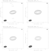 |
Fig. 1. Example CLEANed images of 4C +29.45 at 22 GHz (a), 43 GHz (b), 86 GHz (c), and 129 GHz (d) obtained on 1 March 2016. The map peak fluxes are 2.39, 2.41, 1.84, and 1.25 Jy beam−1 at 22, 43, 86, and 129 GHz. The lowest contour levels are 2.14, 1.32, 2.87, and 7.51% of each map peak flux. Beam sizes are 5.79 × 3.21, 2.93 × 1.58, 1.47 × 0.778, and 0.972 × 0.552 at each frequency. |
2.3. Gaussian model fitting
We fitted the source images with two-dimensional circular Gaussian models. We conducted this using the MODELFIT procedure in DIFMAP until the reduced chi-squares (i.e., a fitting reliability) did not improve significantly compared with the results of the previous fitting iterations and the residual noise became comparable to a uniform distribution similar to the CLEANing procedures. After model fitting, we obtained the best fit model parameters, including the total flux density, Stotal, the peak flux density, Speak, and the size, d, of a circular Gaussian model, as listed in Table A.2. From the obtained model parameters, we estimated the brightness temperature, Tb, of core components using the following equation (Lee et al. 2008):
 (1)
(1)
where k is the Boltzmann constant, Stot is the total flux density in Jy, λ is the observing wavelength in cm, d is the estimated core size in radian, and z is redshift. The estimated brightness temperatures are described in Table A.2 and scaled by 1010 K.
We derived the uncertainties of each observable using the following equations (Fomalont 1999; Lee et al. 2008):
 (2)
(2)
 (3)
(3)
 (4)
(4)
where σpeak, σtotal, and σd are the uncertainties of peak flux density, total flux density, and size, respectively. We regarded the maximum flux and residual noise in the region corresponding to the fitted Gaussian model as Speak and σrms.
2.4. Multiwavelength data
We obtained publicly available data at 15 GHz from the Owens Valley Radio Observatory (OVRO). The 1500 blazar monitoring program at 15 GHz with the 40 m radio telescope at OVRO began in late 2007, approximately one year before the start of the Fermi-LAT science operations (Richards et al. 2011). This monitoring is high cadence, with observations conducted approximately twice a week and with a typical flux uncertainty of 3%. 4C +29.45 has been included in the OVRO sample since early 2008.
In addition, we used 43 GHz VLBI data from the VLBA-BU (Boston University) Blazar Monitoring Program (VLBA-BU-BLAZAR)1. This was obtained using the Very Long Baseline Array (VLBA). We used these data to estimate the size of the emitting regions. The BU blazar group has an ongoing monitoring program that observes a total of 42 γ-ray bright blazars at 43 GHz (Jorstad & Marscher 2016). In this paper, in order to estimate the sizes of emitting regions within the source, we obtained the calibrated visibility (uv) data from the website and fitted the data with two-dimensional circular Gaussian models in a similar way as described in Sect. 2.3.
3. Results and analysis
3.1. Multiwavelength light curves
In order to study the multiwavelength behavior of the source, we compared the light curves at 22, 43, 86, and 129 GHz from the iMOGABA observations with the OVRO (15 GHz) light curve. Although the 15 GHz data were obtained from a single-dish radio telescope with a large beam size and the 22–129 GHz data were obtained using VLBI observations with a small beam size, we can compare the trend of variability, assuming that the emitting region dominating the variability is compact at both scales. We compared the OVRO data with the VLBI flux density obtained by VLBA (Lister et al. 2018), and we found the mean flux ratio between VLBI and single-dish to be 0.9. Thus, we decided to combine the VLBI and single-dish data for the time-series analysis. The combined multifrequency light curves are shown in Fig. 2.
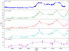 |
Fig. 2. Multiwavelength light curves. From top to the bottom, data frequencies are 15 (obtained from OVRO), 22, 43, 86, and 129 GHz (obtained from the KVN). The dashed lines are to connect the measurements. |
3.1.1. 15 GHz light curve
The 15 GHz light curve of the source is shown in the top panel of Fig. 2. We used 211 epochs over the same period as the KVN observations, from 5 December 2012 (MJD 56266) to 28 December 2016 (MJD 57750). The total flux density was in a range of 0.93–2.42 Jy during the entire observing period. We divided the light curve into two periods, period A and period B. We defined period A as before MJD 56930 and period B as after MJD 56930. The flux density variability of the source is quite different before and after MJD 56930: The source was relatively quiet from MJD 56201 to MJD 56909 (period A). The flux density began to increase gradually after MJD 56930 (period B). During period A, the source flux density was in a range of 0.93–1.24 Jy, with several minor enhancements. The mean flux density during period A was 1.05 Jy, with a standard deviation of 0.07 Jy. During period B, the source became about twice as bright approximately 110 days after MJD 56930, yielding a mean flux density during period B of 1.85 Jy, with a standard deviation of 0.35 Jy. Also, we found three flux enhancements, around MJD 57100, 57300, and 57500, during period B. The flux density increased from 1.01 Jy to 2.42 Jy in the period MJD 56900-57111, from 1.74 Jy to 2.01 Jy in MJD 57229-57282, and from 1.78 Jy to 2.35 Jy in MJD 57416-57552.
3.1.2. 22–129 GHz light curves
The KVN 22–129 GHz light curves are shown in panels (b)-(e) of Fig. 2. The total flux density is in a range of 0.72–2.88 Jy, 0.58–2.66 Jy, 0.26–1.93 Jy, and 0.27–1.26 Jy at 22, 43, 86, and 129 GHz, respectively (Table A.1). The mean flux density (and its standard deviation) is 1.42 Jy (0.62 Jy), 1.28 Jy (0.59 Jy), 0.97 Jy (0.44 Jy), and 0.64 Jy (0.26 Jy) at 22, 43, 86, and 129 GHz, respectively. Consistent with the OVRO light curve, we found that the KVN light curve at 22, 43, and 86 GHz can be divided into two periods. The 129 GHz light curve has fewer data points due to the limitation of the KVN system, and we cannot observe the same behavior as with the lower frequencies.
3.2. Variability timescales
We investigated the variability timescales of the source by decomposing the 15 GHz light curve using a number of combined exponential functions (e.g., Prince et al. 2017). There are several different forms of exponential equations. Valtaoja & Lainela (1999) divided flares into two phases, rising and decaying. Both phases share the peak of the flare, and the ratio between rising and decaying timescales was set to 1.3. In other words, the decaying timescales are 1.3 times longer than their corresponding rising timescales. On the other hand, Prince et al. (2017) combined both rising and decaying phases into one function without fixing the ratio of their timescales. We followed the method in Prince et al. (2017).
We began by fitting the following function to the data (Prince et al. 2017):
![Mathematical equation: $$ \begin{aligned} F(t) = \sum _{i=1}^{n}2F_{0,i} \left[ \mathrm{exp} \left( \frac{t_{0,i} -t}{\tau _{\mathrm{r},i}}\right) + \mathrm{exp} \left( \frac{t-t_{0,i}}{\tau _{\mathrm{d},i}} \right) \right]^{-1} + b. \end{aligned} $$](/articles/aa/full_html/2021/07/aa40198-20/aa40198-20-eq6.gif) (5)
(5)
Here, n is the number of flares, and for individual flares: F0, i is the fitted local maximum flux density, t0, i is the time of the fitted maximum flux density, τr, i is the fitted rising timescale, τd, i is the fitted decaying timescale, and b is a constant flux during our observational period. In order to determine the number of flares, n, to fit the light curve, we made a 30-day running average of the light curve and then defined a flare as being where the flux density was above the average. We have plotted the running average with the light curve in Fig. 3. The fitting algorithm requires initial conditions in order to constrain the fit. Where the flux density was above the average, we set the time of the local peak and the flux density of that peak as the initial conditions for t0, i and F0, i, respectively. We then set the initial conditions for τr, i as the time from when the flux density began to be above the average to the time when it fell back below the average. We found six flares (n = 6) this way. We obtained the best fitting model with a total of 25 free parameters. The results of this fit are summarized in Table 1. The results of the decomposition are shown in Fig. 4, and the reduced chi-squared of this fit was 8.4. It can be seen that the fourth flare potentially has additional structure, so we tried fitting with two functions to this flare. However, due to the lack of the data during the period from MJD 57123 to 57198, the additional flare seems to be constructed with large uncertainty. Therefore, we did not fit any additional functions even though the reduced chi-squared value had improved. The first flare was not well constrained, and we therefore excluded it from our analysis. In the last flare, there was a KVN 22 GHz data point near the fitted peak from this analysis. The KVN data point has a value of 2.88 Jy, which compares well with the fitted values in Table 1, giving us confidence in the accuracy of the fit.
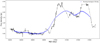 |
Fig. 3. 30-day running average of the OVRO 15 GHz data (blue). A flare was defined as when the light curve was above the running average. The times at which the flux density was above the average and the peak flux density within this time were used as initial conditions for the fitting algorithm described in Sect. 3.2. The dotted lines are to connect the measurements. |
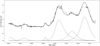 |
Fig. 4. Decomposition of the OVRO light curve with six flares. As we could not constrain the peak for the first flare, we did not use the first flare to estimate the variability brightness temperature, |

Best fitting parameters from the decomposition of the OVRO 15 GHz light curve.
Once we obtained the variability timescales, we were able to estimate the variability brightness temperatures and the variability Doppler factors. The Doppler factor can be estimated if there is a maximum intrinsic brightness temperature ( ) that the source can achieve. The Doppler factor is then proportional to the observed brightness temperature (
 ) using the following equations (Fuhrmann et al. 2008; Rani et al. 2013):
 (6)
(6)
 (7)
(7)
where ΔS is the difference in flux density between the beginning and the peak of a flare, measured in Jy, ν is the observing frequency in GHz (15 GHz), DL = 4477.8 Mpc (assuming Ωm = 0.3 and H0 = 70 km Mpc−1 s−1), τr is the timescale estimated in day, and we assume that the TB, eq is equal to 5 × 10¹⁰ K (Hovatta et al. 2009). A detailed derivation of  is explained in Appendix A. In this estimation, we adopt an e-folding timescale τr,e, which corresponds to the time between the peak of the flare and peak/e. Moreover, we set the flux difference between the peak and peak/e of a flare as ΔS. The estimated variability brightness temperatures and Doppler factors are listed in Table 2.
Estimated variability brightness temperatures and Doppler factors.
In addition, we can estimate the Doppler factors from jet kinematics (e.g., the apparent jet speed, βapp), assuming the critical viewing angle (θ = θcrit) of the jet using the following equations:
 (8)
(8)
 (9)
(9)
 (10)
(10)
 (11)
(11)
In this estimation, we used the maximum apparent speed of βapp = 24.6 ± 2.0 obtained from Lister et al. (2019), assuming the jet viewing angle is at the critical angle, θ = θcrit. We found that the Doppler factor at the critical angle is δcrit = 24.62, which is comparable with the maximum variability Doppler factor of δ = 27.12 ± 3.66 obtained for flare 3 despite the observational periods being different.
3.3. Cross-correlation analysis
In order to investigate a time lag of variations among the multifrequency light curves, we compared the 15 GHz light curve with the 22, 43, and 86 GHz light curves using a discrete cross-correlation function (DCF). In this analysis, we excluded the 129 GHz data because they are very sparse in time and have relatively large errors. The KVN data obtained at 22, 43, and 86 GHz were compared to the OVRO 15 GHz data in this analysis, yielding three data pairs: at 15–22 GHz, 15–43 GHz, and 15–86 GHz. We used the unbinned discrete cross-correlation function (UDCF), in order to avoid interpolating and sampling errors (Edelson & Krolik 1993), following
 (12)
(12)
 (13)
(13)
Here, ai and bj are the ith and jth observed data points,  and
and  are the mean values of data sets a and b, σa and σb are standard deviations of data sets a and b, and ea and eb are measurement errors for the two data sets, respectively. The UDCF is binned with a mean cadence of Δτ = 8 days and the number of data points, M, in the bin to estimate the DCF (Eq. (13)). The statistical uncertainties of the time lag determined from the DCF analysis were obtained by performing a Monte Carlo simulation based on a random subset selection method (Peterson et al. 1998; Lee et al. 2017). Samples of the DCF are shown in the left panels of Fig. 5. A set of N = 1000 randomly sampled light curves was used for determining the correlation peaks, yielding 1000 time delays and their distribution, as shown in the right panels of Fig. 5. By fitting the Gaussian function to the distribution, the statistical uncertainty of the time lag was determined. From the discrete cross-correlation analysis, we found time lags of −54 ± 35, −50 ± 9, and −55 ± 47 days at the 22, 43, and 86 GHz light curves from the 15 GHz light curve, respectively. We also obtained the confidence interval of 95% from −56 to −52, −51 to −49, and −58 to −52 at 15–22, 15–43, and 15–86 GHz, respectively (Lee et al. 2017). We performed this analysis for the whole period since it is hard to distinguish the time lag of individual flares, finding that the radio flux enhancements at 22–86 GHz lead that of the 15 GHz light curve. However, it is hard to compare across the 22–86 GHz range because the KVN observations were conducted simultaneously with a large cadence of about 30 days. Although we are not in a position to distinguish the time lag between the 22 and 86 GHz light curves, the fact that the high frequency (22–86 GHz) light curves lead the 15 GHz light curve implies an opacity effect governing the multifrequency (15 GHz vs. 22 GHz and higher) light curve.
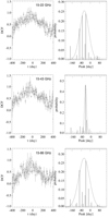 |
Fig. 5. Cross-correlation function and corresponding cross-correlation peak distribution of the light curves in 4C +29.45. Left: sample DCFs at 15–22 GHz (top), 15–43 GHz (middle), and 15–86 GHz (bottom). Right: cross-correlation peak distribution of the corresponding DCFs of 1000 iterations. We fitted the distribution with a Gaussian function in order to specify the mean value and adopt the standard deviation as an uncertainty. |
3.4. Turnover frequency
Synchrotron radiation originates from relativistic electrons traveling in a magnetic field and has an energy distribution of N(E) ∝ E−δ, where N(E) is the electron number density with its energy of E and has a power-law distribution as a function of frequency, S ∝ να, where α is the spectral index. Theoretically, synchrotron emission from an optically thin region has the spectral index of α = (1 − δe)/2, where δe is the Doppler factor of the relativistic electrons, while the emission from the optically thick region has the value of α = 2.5 (Rybicki & Lightman 1979). In order to study the characteristics of the observed synchrotron emitting region, we calculated the spectral indices between each pair of adjacent frequencies. These results are listed in Table 3 and range from −0.4 to 0.1 at 22–43 GHz, from −0.6 to −0.1 at 43–86 GHz, and from −1.6 to 0.1 at 86–129 GHz. We found that the source is optically thinner at higher frequencies and has a flatter spectral index at lower frequencies.
Spectral indices from KVN data.
Synchrotron emission can be absorbed by the same population of synchrotron particles (i.e., electrons) that have the same energy level at low frequencies (e.g., radio frequencies) in the optically thick region. This process is called SSA. Due to the absorption of the synchrotron radiation at lower frequencies, the synchrotron spectrum has a peak at a critical frequency, known as the turnover frequency, νr. This frequency is where the source transitions from being optically thick to optically thin. In order to determine the turnover frequency of the spectrum from the KVN multifrequency observations, we fitted the observed spectra with the following curved power-law function (Algaba et al. 2018b, and references therein):
 (14)
(14)
Here, S(ν) is the flux density at a given frequency, νr is an arbitrary reference frequency, α is the spectral index, Sr is the flux density for when the ν is the same as νr, and b is a constant. Because we wish to find the turnover frequency, we set α to zero. Among the 33 epochs, we selected 13 epochs with available four-frequency measurements and attempted to fit the spectra.
We assumed that the CLEAN fluxes at four KVN frequencies originate from the core, an SSA region. However, in reality, an optically thin, extended jet can contribute to the CLEAN fluxes. The relative contribution of the jet compared with that of the core to the CLEAN fluxes becomes larger at lower frequencies, introducing possible bias to the data. Also, the limited uv coverage of the KVN data may result in an artificial spectral steepening because short baselines could not be sampled at high frequencies (Kim et al. 2018b). We calculated an artificial spectral index of the source following Kim et al. (2018b). In this test, we produced simulated KVN data using the AIPS task UVCON with the Stokes I image FITS data (for epoch of 16 November 2012), obtained from the MOJAVE website2. We found that the artificial spectral index of the source is 0.04, implying that the artificial spectral steepening due to the limited uv coverage of the KVN data is negligible. We also considered an additional uncertainty of 30%, which is obtained from a mean difference between the KVN CLEAN flux density and the BU core flux density selected to have a time difference of less than 7 days at 43 GHz.
We obtained turnover frequencies at 12 epochs, excluding epoch 16 (MJD 56903) during which the fit failed. The fitting results are shown in Fig. 6 and summarized in Table 4. We found that 4C +29.45 has a turnover frequency ranging from 23 GHz to 38 GHz in the period MJD 56381–57750. Since the turnover frequency was measured to be below 43 GHz in all epochs when a successful fit was obtained, based on the curved-power-law fitting analysis, we estimated the optically thin spectral index, αthin, by performing a linear fit to the flux density at 43, 86, and 129 GHz. We found these values to range from −0.74 to −0.25, and the results are shown in Table 4.
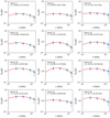 |
Fig. 6. Fitting results of turnover frequencies from KVN four-frequency simultaneous data. The resulting turnover frequencies lie in the range of ∼23−38 GHz. |
Turnover frequency fitting results.
3.5. Magnetic field strength
From the obtained observational parameters, we can estimate the magnetic field strength of an SSA region using the following equation (Marscher 1983; Hodgson et al. 2017):
 (15)
(15)
Here, b(α) is a factor that depends on the spectral index (refer to Table 1 in Marscher 1983). In order to provide a better estimate of b(α) than that given in (Marscher 1983), we linearly interpolated the values listed in Table A.1 in Marscher (1983) and fitted for the optically thin spectral indices found in Sect. 3.4.
In order to estimate the size of the emission region, θr, at the turnover frequency, we first obtained the 43 GHz images of the source from the BU program that were observed both before and after the epochs where the turnover frequency could be measured. We then performed a simple linear interpolation in between these two VLBA epochs in order to determine the size of the 43 GHz core at the epochs where the turnover frequency could be measured. The observed core size is expected to vary as a function of frequency following the relationship
 (16)
(16)
where ϵ represents the geometry of the jet. If the jet is conical, ϵ = 1, and if the jet is parabolic, ϵ = 0.5 (e.g., Algaba et al. 2017). In this case, ϵ was found to be 0.44 ± 0.08 by Algaba et al. (2017). Upper limits of the core size are obtained for three epochs, taking a minimum resolvable size into account (e.g., Lee et al. 2016b). All the uncertainties were obtained using the standard error propagation method, and our derived expressions for calculating the uncertainties are given in Appendix C. Moreover, we can estimate the emission region size, θr, from the variability size, θvar (Hodgson et al. 2020):
 (17)
(17)
In this analysis, we used the variability timescales., τr, e, and the variability Doppler factors, δvar, obtained in Sect. 3.2. Estimated variability sizes are listed in Table 6. Then we extrapolated these variability sizes at turnover frequencies (θvar, νr), taking the jet geometry, ϵ, into account in order to compare the sizes (θVLBI, νr) extrapolated from θVLBI. We found that difference between these sizes is not significant (see Sect. 4.1). Therefore, we adopted the mean size between θvar, νr and θVLBI, νr, regarding the uncertainty as the minimum and maximum of their individual uncertainties. When the variability sizes were not available, we used the extrapolated core sizes, θVLBI, νr (see Sect. 4.1). Our estimated core sizes at the turnover frequency are listed in Table 5.
Estimated B-field strengths of SSA regions.
Size comparison between VLBI measurements and variability.
It should be noted that for the factor  in Eq. (15), we used a power index of −1 instead of the +1 used in Marscher (1983) because we consider that the observables originated from the core region, which is assumed to be relatively stationary in time (Lee et al. 2017; Algaba et al. 2018b). We adopted δ = 9.6 ± 2.6 for the source, as obtained by Jorstad et al. (2017).
Therefore, we obtained seven measurements ranging from  G to
G to  G. For the other epochs, only upper limits could be derived. In this estimation, we excluded epoch 3 (MJD 56349) because the observation was conducted during the first flare and it is hard to constrain the rising timescale (Sect. 3.2). The results of this analysis are shown in Table 5 and Fig. 7.
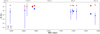 |
Fig. 7. Estimated magnetic field strengths of the SSA region and the energy equipartition region. Filled red circles represent Beq, while filled blue circles represent BSSA. Triangles are lower limits, and inverted triangles are upper limits. The lower uncertainty of BSSA is computed in logarithm (see Appendix C). |
In addition to the magnetic field strength, BSSA, of an SSA region, we can also estimate the minimum magnetic field strength, Beq, assuming equipartition between magnetic field and particle energy densities. The expression to describe this is as follows (Kataoka & Stawarz 2005; Algaba et al. 2018a):
 (18)
(18)
Here, η is a ratio between the energies of hadrons and leptons: η is 1 for a leptonic model and 1836 for a hadronic model. In this analysis, we adopted a compromise value of η ≈ 100 because we do not know the true composition of the jet. For the same reasons as before, the equipartition magnetic field strength could only be determined for eight epochs. The equipartition magnetic field strengths were found to range from 0.10 ± 0.03 G to 0.25 ± 0.07 G. These values are generally up to two orders of magnitudes stronger than BSSA, except for two epochs (MJD 56616 and MJD 56651), where BSSA and Beq are approximately comparable within uncertainties. The results are shown in Table 5 and Fig. 7.
The magnetic field strength of a core region in the jet can be estimated from a core-shift effect, as described in Lobanov (1998) and Pushkarev et al. (2012). Assuming equipartition between particle and magnetic field energy densities, a spectral index of α = −0.5 (Sν ∝ να), and a critical angle θ ≈ Γ−1, the magnetic field strength at a distance of 1 pc from the central engine is given by:
 (19)
(19)
where z is redshift, βapp is apparent jet speed, and Ωrν is the core shift measure defined in Lobanov (1998) as
 (20)
(20)
where Δrc is the core shift between different frequencies ν1 and ν2 (ν1 < ν2). The magnetic field strength Bc at a core region rc observed by VLBI observations can be estimated as  . The distance rc of the core from the central engine is given by Lobanov (1998) as
 (21)
(21)
where ν is a given frequency. From the study on the core shift variability of the relativistic jets (Plavin et al. 2019), we found that 4C +29.45 had a core shift of 1.02 mas measured at ν1 = 2.3 GHz and ν2 = 6.8 GHz on 5 December 2012 (MJD 56266), which is the closest measurement in time to our analysis. The core shift gives us a core shift measure of Ωrν = 23.4 pc GHz and a magnetic field strength at 1 pc of B1 = 1.25 G, taking the apparent speed of the jet, βapp = 24.6, into account (Lister et al. 2019). In order to compare the magnetic field strength Bc from the core shift to that of the SSA region, BSSA, we estimated the core distance rc(νr) = 19.14 pc at a turnover frequency of νr = 30.09 GHz (measured on MJD 56381). We found the magnetic field strength of the core region to be Bc = 0.065 G, which is an order of magnitude higher than the BSSA = 0.006 G measured on MJD 56381.
4. Discussion
4.1. Testing our assumptions on the size estimates
According to Eq. (15) (for estimating BSSA), the emission size θr is one of the important factors for BSSA estimates ( ) and hence the uncertainty of the emission size. The determination of θr, presented in Sect. 3.5, relies on two assumptions. Firstly, the variability size (e.g., θvar) is, in principle, an intrinsic size of a variable emission region (e.g., a VLBI core) and a high resolution VLBI observation may be able to resolve the emission region size (e.g., θVLBI). Therefore, at a given frequency ν, those sizes are comparable (θvar, ν ≈ θVLBI, ν) if the VLBI observations can resolve the emission region. Secondly, a jet transverse radius R (or a jet angular size θ) expands along the distance r of a VLBI core from the central engine (R ∝ rϵ or θ ∝ rϵ), and the distance of the core (i.e., an optical depth τ = 1 surface of an emission region in the jet) depends on the observing frequency ν (r ∝ ν−1). Therefore, the jet geometry assumption θ ∝ ν−ϵ used to extrapolate the sizes to the turnover frequency is valid.
If we have a variability size θvar measured at a frequency ν1 and a VLBI size θVLBI observed at another frequency, ν2, we then expect that extrapolated sizes θvar, ν3 and θVLBI, ν3 at a common frequency, ν3, are comparable. In this study, we obtained θVLBI from VLBA observations at 43 GHz and θvar from the variability timescales at 15 GHz. In order to check these assumptions, we extrapolated the sizes at turnover frequencies based on the jet geometry ϵ = 0.44. We found that the estimated variability sizes were generally comparable with the sizes observed directly by VLBI observations as shown in Fig. 8. In order to specify the differences between θvar, νr and θVLBI, νr, we performed a linear fit to the data for five epochs (Fig. 8). The fitting result shows a slope of 1.05 ± 0.23 between θvar, νr and θVLBI, νr, although one data point for one epoch does not follow this trend. This implies that the assumptions on the size estimation are valid. Therefore, we decided to use the mean value of the two sizes, taking the uncertainties into account. However, for the other six epochs we decided to use the θVLBI, νr because it is hard to constrain the correlation due to the time gap between those two sizes.
 |
Fig. 8. Comparison between extrapolated sizes θvar, νr and θVLBI, νr at turnover frequency from θvar, 15 and θVLBI, 43 based on the jet geometry ϵ = 0.44 (Algaba et al. 2017). The solid line represents the result of the linear fitting (as also described at the top of the figure). |
4.2. Brightness temperature
We obtained the brightness temperatures from the KVN data (Table A.2). The median brightness temperatures obtained from model-fitting the KVN data are shown in Table A.2. We found a significant (> 3σ) trend of decreasing brightness temperature with increasing frequency. In the previous studies analyzing KVN observations, we see increasing brightness temperatures with increasing observing frequency because the beam size decreases with increasing observing frequency (Lee et al. 2016b; Algaba et al. 2019). Because of the large KVN beam size leading to a larger core blending effect at lower frequencies, the KVN beam does not resolve the core at the lower frequency. Therefore, the brightness temperature of the core was underestimated due to the larger source size measured. This effect becomes weaker at higher frequency observations that have relatively small beam sizes. In contrast to this, our results show an opposite tendency of brightness temperature to the previous studies that used KVN observations; however, our results are consistent with a previous study on the intrinsic brightness temperature evolution as a function of observing frequency using high angular-resolution VLBI observations (Lee 2014). According to Lee (2014), the intrinsic brightness temperature, T0, of relativistic jets decreases following  with νobs ≥ 9 GHz. In order to check the power index of TB, we selected 14 epochs during which the core sizes were estimated larger than minimum resolvable sizes at more than three frequencies. We found a decreasing trend of core sizes with the observing frequencies in 14 epochs and then fitted the TB calculated by these core sizes. We obtained a mean index of −1.50 ± 0.21 (weighted average of −1.11) by excluding minimum resolvable sizes, which is a comparable result to that estimated in Lee (2014). Although we are not in a position to directly derive the intrinsic brightness temperature of the relativistic jet using these KVN observations, this result leads us to conclude that the KVN observations of the source are less affected by core blending effects for 4C +29.45 compared with past KVN observations of other sources.
For VLBI observations with limited visibility data, we can use a new approach for estimating brightness temperature that is based on individual visibility measurements and their errors following Lobanov (2015). We can estimate a brightness temperature limit (TB, lim) as described by Eq. (5) in Lobanov (2015):
 (22)
(22)
 (23)
(23)
We selected KVN observations on MJD 56771, 57037, 57290, and 57503 (the closest epochs to flares 3–6) and estimated the brightness temperature limits at various frequencies as summarized in Table 7. We found that the estimated brightness temperature limits (TB, lim) are comparable to those TB obtained from KVN images, yielding a ratio of TB, lim/TB = 1.82−4.76. This is consistent with the application results of TB, lim/TB = 4.6 for the MOJAVE data as reported in Lobanov (2015).
Brightness temperatures.
As another way of measuring the brightness temperature of the nonthermal synchrotron emission from the relativistic jets, we investigated the variability brightness temperatures,  , from the obtained variability timescales in Table 2. We found that the mean variability brightness temperature is much higher than the mean brightness temperature derived from the KVN images at 22 GHz and those (Table 7) obtained by applying the approach in Lobanov (2015). In order to understand where this difference comes from, we calculated the size of the emission region, θvar, from the variability properties as described in Sect. 3.5 and compared these θvar values with the size of the radio core emission regions obtained from the KVN images. The mean core sizes are 0.47 ± 0.25 mas, 0.53 ± 0.22 mas, 0.42 ± 0.17 mas, and 0.37 ± 0.34 mas at 22, 43, 86, and 129 GHz, respectively. The obtained mean variability size derived from the 15 GHz observations is 0.088 ± 0.034 mas, which is smaller than the KVN size at 22 GHz by a factor of five. Therefore, we postulate that this core size discrepancy may partially affect the difference between brightness temperatures at 22–129 GHz and the variability brightness temperatures at 15 GHz.
4.3. Variability behavior
We divided the radio light curve into two distinct periods: part A and part B (Fig. 2). We attempted to investigate if there are any physical changes in the source over this period.
We cross-compared the flux densities with derived parameters, such as core sizes, turnover frequencies, and Doppler factors, yielding no cross-correlation between the parameters. In particular, as shown in Table 2, we did not find any obvious trend in the Doppler factors in Sect. 3.2. Similarly, we found no obvious trend in the variability brightness temperatures. This may imply that the strong flaring activities in 4C +29.45 are not attributable to the Doppler factor variability. However, it must be noted that the Doppler factor estimates rely on an intrinsic brightness temperature assumption. It could be that the intrinsic brightness temperature is changing and therefore the Doppler factors as well. We intend to resolve this degeneracy in our future work (Kang et al., in prep.).
We also compared the OVRO data with other published multiwavelength data, including data from the Fermi-gamma-ray space telescope AGN multifrequency monitoring alliance (F-GAMMA; Angelakis et al. 2019) and polarimetric monitoring of AGN at millimeter wavelengths (POLAMI; Agudo et al. 2018) projects and the submillimeter array (SMA) monitoring program. We found that two flares (flares 2 and 3) seem to appear in the F-GAMMA (23 and 43 GHz) and POLAMI (86 and 230 GHz) light curves. We found that three flares (flares 3, 4, and 5) include the flux enhancements that appeared in the SMA light curve (230 GHz). For flare 2, the multiwavelength flux densities peaked quasi-simultaneously around MJD 56500 at 15, 43, 86, and 230 GHz. The spectrum seems to be inverted between 15 and 43 GHz and steep between 43 and 230 GHz. On the other hand, for flare 3 the multiwavelength light curves at 43, 86, and 230 GHz seemed to peak earlier than the OVRO 15 GHz light curve. Moreover, the spectrum may appear to be inverted between 15 and 86 GHz and steep between 86 and 230 GHz. Although we are not in a position to accurately analyze the multiwavelengths data at 15–230 GHz, the comparison results may imply that during the period of flares 2 and 3 the inverted spectrum (optically thick spectrum) extends to a higher frequency (hence a higher turnover frequency) and that the high energy synchrotron particles increased from flare 2 to flare 3 (before the source entered period B).
5. Conclusions
We studied the long-term behavior of blazar 4C +29.45, which was observed from December 2012 to December 2016. We analyzed KVN data with OVRO 15 GHz data. We found that the OVRO 15 GHz light curve can be divided into two distinguishable periods, period A and period B, and also found similar variation trends in the 22, 43, and 86 GHz light curves. In order to confirm the characteristics of the variation, we attempted to estimate the variability timescales using a combined exponential function. We also estimated turnover frequencies and maximum flux densities with 22, 43, 86, and 129 GHz KVN data. Then we estimated BSSA using turnover frequencies and maximum flux densities, with core sizes from BU data and the Doppler factor of δ = 9.6 from Jorstad et al. (2017). The BSSA ranged from 0.001 to 0.099 G. In our analysis, we used upper limits for core sizes. In addition, we estimated Beq assuming η ∼ 100 (i.e., assuming the jet consists of electrons with both positrons and protons). The Beq ranged from 0.10 to 0.25 G and are much greater than the BSSA for all periods, although we assumed the upper limits and lower limits of BSSA and Beq, respectively. From the results we concluded that the equipartition region is located upstream from the SSA region.
Meanwhile, Fermi-LAT reported an intense flare of gamma-ray emission from 4C +29.45 in October 2015 (Prince 2019). We will discuss the correlation between the gamma-ray flare and the behavior of radio emission, such as variation in core sizes and flux density, in a follow-up study.
Acknowledgments
We would like to thank the anonymous referee for important comments and suggestions that have enormously improved the manuscript. J.-C. Algaba acknowledges support from the Malaysian Fundamental Research Grant Scheme (FRGS)FRGS/1/2019/STG02/UM/02/6. This work was supported by the National Research Foundation of Korea (NRF) grant funded by the Korea government (MIST) (2020R1A2C2009003). We are grateful to the staff of the KVN who helped to operate the array and to correlate the data. The KVN and a high-performance computing cluster are facilities operated by the KASI (Korea Astronomy and Space Science Institute). The KVN observations and correlations are supported through the high-speed network connections among the KVN sites provided by the KREONET (Korea Research Environment Open NETwork), which is managed and operated by the KISTI (Korea Institute of Science and Technology Information). This research has made use of data from the OVRO 40-m monitoring program (Richards, J. L. et al. 2011, ApJS, 194, 29) which is supported in part by NASA grants NNX08AW31G, NNX11A043G, and NNX14AQ89G and NSF grants AST-0808050 and AST-1109911. This study makes use of 43 GHz VLBA data from the VLBA-BU Blazar Monitoring Program (VLBA-BU-BLAZAR (http://www.bu.edu/blazars/VLBAproject.html), funded by NASA through the Fermi Guest Investigator Program. The VLBA is an instrument of the National Radio Astronomy Observatory. The National Radio Astronomy Observatory is a facility of the National Science Foundation operated by Associated Universities, Inc. This research has made use of data from the MOJAVE database that is maintained by the MOJAVE team (Lister et al. 2018). J.P. acknowledges financial support from the Korean National Research Foundation (NRF) via Global PhD Fellowship grant 2014H1A2A1018695 and support through the EACOA Fellowship awarded by the East Asia Core Observatories Association, which consists of the Academia Sinica Institute of Astronomy and Astrophysics, the National Astronomical Observatory of Japan, Center for Astronomical Mega-Science, Chinese Academy of Sciences, and the Korea Astronomy and Space Science Institute. Jeffrey Hodgson is supported via the National Research Foundation of Korea (NRF) grant (2021R1C1C1009973). D. Kim and S. Trippe acknowledge support via NRF grant 2019R1F1A1059721.
References
- Agudo, I., Thum, C., Ramakrishnan, V., et al. 2018, MNRAS, 473, 1850 [Google Scholar]
- Aharonian, F., Akhperjanian, A. G., Bazer-Bachi, A. R., et al. 2007, ApJ, 664, L71 [Google Scholar]
- Algaba, J.-C., Gabuzda, D. C., & Smith, P. S. 2012, MNRAS, 420, 542 [Google Scholar]
- Algaba, J.-C., Zhao, G.-Y., Lee, S.-S., et al. 2015, JKAS, 48, 237 [Google Scholar]
- Algaba, J.-C., Nakamura, M., Asada, K., et al. 2017, ApJ, 834, 65 [Google Scholar]
- Algaba, J.-C., Lee, S.-S., Rani, B., et al. 2018a, ApJ, 859, 128 [Google Scholar]
- Algaba, J.-C., Lee, S.-S., Kim, D.-W., et al. 2018b, ApJ, 852, 30 [Google Scholar]
- Algaba, J.-C., Hodgson, J., Kang, S., et al. 2019, JKAS, 52, 31 [Google Scholar]
- Angel, J., & Stockman, H. 1980, ARA&A, 1980, 321 [Google Scholar]
- Angelakis, E., Fuhrmann, L., Myserlis, I., et al. 2019, A&A, 626, A60 [CrossRef] [EDP Sciences] [Google Scholar]
- Asada, K., & Nakamura, M. 2012, ApJ, 745, L28 [NASA ADS] [CrossRef] [Google Scholar]
- Asada, K., Nakamura, M., Doi, A., Nagai, H., & Inoue, M. 2014, ApJ, 781, L2 [NASA ADS] [CrossRef] [Google Scholar]
- Begelman, M. C., Blandford, R. D., & Rees, M. J. 1984, Rev. Mod. Phys., 56, 255 [Google Scholar]
- Edelson, R. A., & Krolik, J. H. 1993, ApJ, 333, 646 [Google Scholar]
- Event Horizon Telescope Collaboration (Akiyama, K., et al.) 2019, ApJ, 875, L1 [NASA ADS] [CrossRef] [Google Scholar]
- Fomalont, E. B. 1999, Synthesis Imaging in Radio Astronomy II, 180, 301 [Google Scholar]
- Fuhrmann, L., Krichbaum, T. P., Witzel, A., et al. 2008, A&A, 490, 1019 [NASA ADS] [CrossRef] [EDP Sciences] [Google Scholar]
- Gabuzda, D. 2017, Galaxies, 5, 11 [Google Scholar]
- Hales, C. A., Beneglia, P., del Palacio, S., et al. 2017, A&A, 598, A42 [NASA ADS] [CrossRef] [EDP Sciences] [Google Scholar]
- Hada, K., Kino, M., Doi, A., et al. 2016, ApJ, 817, 131 [Google Scholar]
- Hodgson, J., Lee, S.-S., Zhao, G.-Y., et al. 2016, JKAS, 49, 137 [Google Scholar]
- Hodgson, J., Krichbaum, T. P., Marscher, A. P., et al. 2017, A&A, 597, A80 [NASA ADS] [CrossRef] [EDP Sciences] [Google Scholar]
- Hodgson, J., Rani, B., Lee, S.-S., et al. 2018, MNRAS, 475, 368 [Google Scholar]
- Hodgson, J., L’Huillier, B., Liodakis, I., et al. 2020, MNRAS, 495, L27 [Google Scholar]
- Homan, D. C., Lister, M. L., Kovalev, Y. Y., et al. 2015, ApJ, 798, 134 [Google Scholar]
- Hovatta, T., Valtaoja, E., Tornikoski, M., & Lähteenmäki, A. 2009, A&A, 494, 527 [NASA ADS] [CrossRef] [EDP Sciences] [Google Scholar]
- Jorstad, S., & Marscher, A. 2016, Galaxies, 4, 47 [Google Scholar]
- Jorstad, S., Marscher, A., Morozova, D., et al. 2017, ApJ, 846, 98 [Google Scholar]
- Kataoka, J., & Stawarz, L. 2005, ApJ, 622, 797 [Google Scholar]
- Kim, D.-W., Trippe, S., Lee, S.-S., et al. 2017, JKAS, 50, 167 [Google Scholar]
- Kim, J.-Y., Krichbaum, T. P., Lu, R.-S., et al. 2018a, A&A, 616, A188 [NASA ADS] [CrossRef] [EDP Sciences] [Google Scholar]
- Kim, J.-Y., Lee, S.-S., Hodgson, J., et al. 2018b, A&A, 610, L5 [EDP Sciences] [Google Scholar]
- Kim, D.-W., Trippe, S., Lee, S.-S., et al. 2018c, MNRAS, 480, 2324 [Google Scholar]
- Komissarov, S. S., Barkov, M. V., Vlahakis, N., & Königl, A. 2007, MNRAS, 380, 51 [Google Scholar]
- Kovalev, Y. Y., Lobanov, A. P., Pushkarev, A. B., & Zensus, J. A. 2008, A&A, 483, 759 [NASA ADS] [CrossRef] [EDP Sciences] [Google Scholar]
- Lee, S.-S. 2014, JKAS, 47, 303 [Google Scholar]
- Lee, S.-S., Lobanov, A. P., Krichbaum, T. P., et al. 2008, AJ, 136, 159 [Google Scholar]
- Lee, S.-S., Petrov, L., Byun, D.-Y., et al. 2014, AJ, 147, 77 [Google Scholar]
- Lee, S.-S., Lobanov, A. P., Krichbaum, T. P., & Zensus, J. A. 2016a, ApJ, 826, 135 [Google Scholar]
- Lee, S.-S., Wajima, K., Algaba, J.-C., et al. 2016b, ApJS, 227, 8 [Google Scholar]
- Lee, J. W., Lee, S.-S., Hodgson, J., et al. 2017, ApJ, 841, 119 [Google Scholar]
- Lee, J. W., Lee, S.-S., Algaba, J.-C., et al. 2020, ApJ, 902, 104 [Google Scholar]
- Lister, M. L., Aller, M. F., Aller, H. D., et al. 2018, ApJS, 234, 12 [NASA ADS] [CrossRef] [Google Scholar]
- Lister, M. L., Homan, D. C., Hovatta, T., et al. 2019, ApJ, 874, 43 [NASA ADS] [CrossRef] [Google Scholar]
- Liu, B.-R., Liu, X., Marchili, N., et al. 2013, A&A, 555, A134 [NASA ADS] [CrossRef] [EDP Sciences] [Google Scholar]
- Lobanov, A. P. 1998, A&A, 330, 79 [NASA ADS] [Google Scholar]
- Lobanov, A. P. 2015, A&A, 574, A84 [NASA ADS] [CrossRef] [EDP Sciences] [Google Scholar]
- Madau, P., Ghisellini, G., & Persic, M. 1987, MNRAS, 224, 257 [Google Scholar]
- Marscher, A. P. 1983, ApJ, 264, 296 [NASA ADS] [CrossRef] [Google Scholar]
- Marscher, A. P., Jorstad, S. G., D’Arcangelo, F. D., et al. 2008, Natur, 452, 966 [Google Scholar]
- Martí-Vidal, I., Krichbaum, T. P., Marscher, A. P., et al. 2012, A&A, 542, A107 [NASA ADS] [CrossRef] [EDP Sciences] [Google Scholar]
- Mertens, F., Lobanov, A. P., Walker, R. C., & Hardee, P. E. 2016, A&A, 595, A54 [NASA ADS] [CrossRef] [EDP Sciences] [Google Scholar]
- Nakamura, M., & Asada, K. 2013, ApJ, 755, 118 [Google Scholar]
- Nakamura, M., Asada, K., Hada, K., et al. 2018, ApJ, 868, 146 [Google Scholar]
- Park, J., Hada, K., Kino, M., et al. 2019a, ApJ, 871, 257 [Google Scholar]
- Park, J., Lee, S.-S., Kim, J.-Y., et al. 2019b, ApJ, 877, 106 [NASA ADS] [CrossRef] [Google Scholar]
- Park, J., Hada, K., Kino, M., et al. 2019c, ApJ, 887, 147 [Google Scholar]
- Peterson, B. M., Wanders, I., Horne, K., et al. 1998, PASP, 110, 660 [NASA ADS] [CrossRef] [Google Scholar]
- Plavin, A. V., Kovalev, Y. Y., Pushkarev, A. B., & Lobanov, A. P. 2019, MNRAS, 485, 1822 [NASA ADS] [CrossRef] [Google Scholar]
- Prince, R. 2019, ApJ, 871, 101 [Google Scholar]
- Prince, R., Majumdar, P., & Gupta, N. 2017, ApJ, 844, 62 [Google Scholar]
- Pushkarev, A. B., Hovatta, T., Kovalev, Y. Y., et al. 2012, A&A, 545, A113 [NASA ADS] [CrossRef] [EDP Sciences] [Google Scholar]
- Raiteri, C. M., Villata, M., & D’Ammando, F. 2013, MNRAS, 436, 1530 [Google Scholar]
- Rani, B., Krichbaum, T. P., & Fuhrmann, L. 2013, A&A, 552, A11 [NASA ADS] [CrossRef] [EDP Sciences] [Google Scholar]
- Richards, J. L., Max-Moerbeck, W., Pavlidou, V., et al. 2011, ApJS, 194, 29 [Google Scholar]
- Rybicki, G. B., & Lightman, A. P. 1979, Radiative Processes in Astrophysics (New York: Wiley) [Google Scholar]
- Valtaoja, E., & Lainela, M. 1999, ApJS, 120, 95 [Google Scholar]
- Véron-Cetty, M.-P., & Véron, P. 2010, A&A, 518, A10 [NASA ADS] [CrossRef] [EDP Sciences] [Google Scholar]
- Wang, J.-Y., An, T., Baan, W. A., et al. 2014, MNRAS, 443, 58 [Google Scholar]
- Zhao, W., Hong, X.-Y., An, T., et al. 2011, A&A, 529, A113 [NASA ADS] [CrossRef] [EDP Sciences] [Google Scholar]
- Zhao, G.-Y., Jung, T., Richard, D., et al. 2015, PKAS, 30, 629 [Google Scholar]
Appendix A: Image and MODELFIT parameters from KVN observations.
The image and MODELFIT parameters obtained from KVN observations, as described in Sect. 2, are summarized in Tables A.1 and A.2.
Image Parameters from KVN Observations.
MODELFIT parameters from KVN Observations.
Appendix B: Brightness temperature
The definition of brightness temperature is as follows:
 (B.1)
(B.1)
Under the Rayleigh-Jeans approximation, this simplifies to
 (B.2)
(B.2)
The intensity Iν can be defined as S/Ω, where Ω is πθ2/4ln2 in circular Gaussian structure. Therefore, we can write the equation as
 (B.3)
(B.3)
In order to estimate the brightness temperature, assuming that the emission is dominated by the variability emission region, we can estimate the variability size as
 (B.4)
(B.4)
If we replace θ with θvar, we obtain
 (B.5)
(B.5)
Here, ν is the frequency in the rest frame. We can convert it to the observer’s frame by inferring ν = νobs(1 + z) and DA = DL/(1 + z)2, thus obtaining:
 (B.6)
(B.6)
Computing the numerical factor, we obtain a final, convenient expression of
Computed numerical factors between two different sets of units for brightness temperature estimation.
![Mathematical equation: $$ \begin{aligned} T_{\rm B}^\mathrm{var}\!=\!4.077\times 10^{13}\! \left(\frac{D_{\rm L}}{[\mathrm {Mpc}]}\right)^2\! \!\left(\frac{\nu _{\rm obs}}{[\mathrm GHz]}\right)^{-2} \!\!\left(\frac{\Delta t}{[\mathrm {day}]}\right)^{-2}\! \frac{S}{(1+z)^4}. \end{aligned} $$](/articles/aa/full_html/2021/07/aa40198-20/aa40198-20-eq68.gif) (B.7)
(B.7)
Appendix C: Error propagation
We estimated the uncertainty of the magnetic field strength using basic error propagation. When the magnetic field strength, B, is estimated by Ab (i.e., B ∝ Ab), the uncertainty, σB, can be calculated as  . Therefore, the uncertainty of the magnetic field strength in SSA, σBSSA, is proportional to
  and
and  , and the uncertainty of magnetic field strength in equipartition, σBeq, is proportional to
  and
and  . Moreover, the lower uncertainty of BSSA is larger than BSSA itself (e.g., BSSA < σBSSA). Therefore we compute the lower uncertainty of BSSA in logarithm as follows:
 (C.1)
(C.1)
 (C.2)
(C.2)
All Tables
Computed numerical factors between two different sets of units for brightness temperature estimation.
All Figures
|
Fig. 1. Example CLEANed images of 4C +29.45 at 22 GHz (a), 43 GHz (b), 86 GHz (c), and 129 GHz (d) obtained on 1 March 2016. The map peak fluxes are 2.39, 2.41, 1.84, and 1.25 Jy beam−1 at 22, 43, 86, and 129 GHz. The lowest contour levels are 2.14, 1.32, 2.87, and 7.51% of each map peak flux. Beam sizes are 5.79 × 3.21, 2.93 × 1.58, 1.47 × 0.778, and 0.972 × 0.552 at each frequency. |
| In the text | |
|
Fig. 2. Multiwavelength light curves. From top to the bottom, data frequencies are 15 (obtained from OVRO), 22, 43, 86, and 129 GHz (obtained from the KVN). The dashed lines are to connect the measurements. |
| In the text | |
|
Fig. 3. 30-day running average of the OVRO 15 GHz data (blue). A flare was defined as when the light curve was above the running average. The times at which the flux density was above the average and the peak flux density within this time were used as initial conditions for the fitting algorithm described in Sect. 3.2. The dotted lines are to connect the measurements. |
| In the text | |
|
Fig. 4. Decomposition of the OVRO light curve with six flares. As we could not constrain the peak for the first flare, we did not use the first flare to estimate the variability brightness temperature, |
| In the text | |
|
Fig. 5. Cross-correlation function and corresponding cross-correlation peak distribution of the light curves in 4C +29.45. Left: sample DCFs at 15–22 GHz (top), 15–43 GHz (middle), and 15–86 GHz (bottom). Right: cross-correlation peak distribution of the corresponding DCFs of 1000 iterations. We fitted the distribution with a Gaussian function in order to specify the mean value and adopt the standard deviation as an uncertainty. |
| In the text | |
|
Fig. 6. Fitting results of turnover frequencies from KVN four-frequency simultaneous data. The resulting turnover frequencies lie in the range of ∼23−38 GHz. |
| In the text | |
|
Fig. 7. Estimated magnetic field strengths of the SSA region and the energy equipartition region. Filled red circles represent Beq, while filled blue circles represent BSSA. Triangles are lower limits, and inverted triangles are upper limits. The lower uncertainty of BSSA is computed in logarithm (see Appendix C). |
| In the text | |
|
Fig. 8. Comparison between extrapolated sizes θvar, νr and θVLBI, νr at turnover frequency from θvar, 15 and θVLBI, 43 based on the jet geometry ϵ = 0.44 (Algaba et al. 2017). The solid line represents the result of the linear fitting (as also described at the top of the figure). |
| In the text | |
Current usage metrics show cumulative count of Article Views (full-text article views including HTML views, PDF and ePub downloads, according to the available data) and Abstracts Views on Vision4Press platform.
Data correspond to usage on the plateform after 2015. The current usage metrics is available 48-96 hours after online publication and is updated daily on week days.
Initial download of the metrics may take a while.