| Issue |
A&A
Volume 650, June 2021
|
|
|---|---|---|
| Article Number | A187 | |
| Number of page(s) | 16 | |
| Section | Stellar structure and evolution | |
| DOI | https://doi.org/10.1051/0004-6361/202140300 | |
| Published online | 29 June 2021 | |
Nucleosynthesis constraints through γ-ray line measurements from classical novae
Hierarchical model for the ejecta of 22Na and 7Be
Center for Astrophysics and Space Sciences, University of California, San Diego, 9500 Gilman Dr, 92093-0424 La Jolla, USA
e-mail: This email address is being protected from spambots. You need JavaScript enabled to view it.
Received:
7
January
2021
Accepted:
4
April
2021
Abstract
Context. Classical novae belong to the most frequent transient events in the Milky Way and are key agents of ongoing nucleosynthesis. Despite their large numbers, they have never been observed in soft γ-ray emission. Measurements of their γ-ray signatures would provide insights into explosion mechanism and nucleosynthesis products.
Aims. Our goal is to constrain the ejecta masses of 7Be and 22Na from classical novae through their γ-ray line emissions at 478 and 1275 keV.
Methods. We extracted posterior distributions on the line fluxes from archival data of the INTEGRAL/SPI spectrometer telescope. We then used a Bayesian hierarchical model to link individual objects and diffuse emission, and to infer ejecta masses from the whole population of classical novae in the Galaxy.
Results. Individual novae are too dim to be detectable in soft γ-rays, and the upper bounds on their flux and ejecta mass uncertainties cover several orders of magnitude. Within the framework of our hierarchical model, we can nevertheless infer tight upper bounds on the 22Na ejecta masses, given all uncertainties from individual objects as well as diffuse emission, of < 2.0 × 10⁻⁷ M⊙ (99.85th percentile).
Conclusions. In the context of ONe nucleosynthesis, the 22Na bounds are consistent with theoretical expectations and exclude that most ONe novae occur on white dwarfs with masses of about 1.35 M⊙. The upper bounds from 7Be are uninformative. From the combined ejecta mass estimate of 22Na and its β+ decay, we infer a positron production rate of < 5.5 × 1042 e+ s−1, which would mean 10% at most of the total annihilation rate in the Milky Way.
Key words: gamma rays: general / methods: statistical / novae, cataclysmic variables / stars: abundances / ISM: abundances
© ESO 2021
1. Introduction
Classical novae (CNe) are thermonuclear explosions on the surface of white dwarfs (WDs) and belong to the most frequent transient phenomena within a galaxy. Despite their high occurrence rate in the Milky Way of 50 ± 25 yr−1 (Shafter 2017), only about 20% are seen in UVOIR wavelengths in one year. At X-ray (Ness et al. 2007) and GeV (Franckowiak et al. 2018) energies, only a few dozen objects in total could be analysed in detail to date. At MeV energies, CNe have never been observed, leaving a large gap in the understanding of nucleosynthesis in these events, as well as in the transition region between thermal and non-thermal processes.
The absolute nucleosynthesis yields from CNe are very uncertain and have only been inferred indirectly from abundance ratios in the expanding nova clouds, the latter of which generally agree very well with theoretical expectations (e.g., Livio & Truran 1994). The interiors of these objects can be studied using γ-rays, and absolute abundances can be determined (e.g., Clayton & Hoyle 1974; Clayton 1981; Leising & Clayton 1987; Hernanz & José 2006; Hernanz et al. 2014). The most promising messengers of ongoing nucleosynthesis in CNe include 7Be and 22Na, which emit soft γ-rays at 478 keV and 1275 keV, respectively, as by-products of the decays to their stable daughter-nuclei 7Li and 22Ne.
Individual objects are too dim for the best current γ-ray line spectrometer telescope, INTEGRAL/SPI (Winkler et al. 2003; Vedrenne et al. 2003), to be detected beyond a few hundred parsec (pc). Because many objects contribute to the total Galactic luminosity, however, we have attempted to constrain the ejecta masses of 7Be and 22Na from the whole population of known and unknown CNe. The cumulative effect of this population of sub-threshold sources is expected to result in a radioactive glow along the Galactic plane in both isotopes. This effect is well measured in the case of 26Al from the nucleosynthesis within massive stars (e.g., Diehl et al. 2006; Bouchet et al. 2015; Pleintinger et al. 2019). In the case of CNe, earlier measurements with COMPTEL focused on the diffuse emission of the 1275 keV line. In the inner Galaxy (|l|< 30°), Jean et al. (2001) found in an upper limit of the 22Na ejecta mass from the diffuse emission of ONe novae (see Sect. 2.1) of < 3 × 10⁻⁷ M⊙. The strongest constraints so far for an individual object were found by Iyudin et al. (1999), with a limit of < 2.1 × 10⁻⁸ M⊙ from Nova Cygni 1992. A similar but rougher extended emission can also be expected from the 478 keV line, which has not been considered yet, however. The most stringent upper bound on the ejecta mass of 7Be was found by Siegert et al. (2018) for the CO nova V5668 Sgr, with < 1.2 × 10⁻⁸ M⊙, assuming a distance of 1.6 kpc. All these limits are close to the highest ejecta mass estimates, for example from UV measurements (e.g., Molaro et al. 2016, finding < 0.7 × 10⁻⁸ M⊙ for V5668 Sgr), which rely on a canonical value for the total ejecta mass, however, which itself is uncertain by one order of magnitude.
In addition to the diffuse part, more than 100 individual CNe are known to have occurred during the time of the INTEGRAL observations since 2003. Their contribution must therefore also be taken into account. This is possible in the framework of a Bayesian hierarchical model (Gelman et al. 2013) in which we attempt to link the physics of individual CNe and thus determine ejecta mass estimates from the whole CN population for both CO and ONe novae.
This paper is structured as follows: in Sect. 2 we introduce the nucleosynthesis that is expected to occur in CNe and predict individual and cumulative γ-ray signals from these expectations in general. Sect. 3 describes the INTEGRAL/SPI data set, followed by Sect. 4, which includes the sample of known CNe during the time of the observations. The general data analysis for extracting fluxes from the raw count data is shown in Sect. 5, together with the refined approach of the Bayesian hierarchical model. We present our results from individual sources, diffuse emission, and hierarchical modelling in Sect. 6. In Sect. 7 we discuss these results in terms of CN nucleosynthesis constraints and the contribution of ONe novae to the Galactic positron puzzle. We summarise and conclude in Sect. 8.
2. Nuclear astrophysics expectations for novae
2.1. Explosive burning
Nova explosions are the result of mass accretion onto a WD in a close binary system. The explosion itself is described as a thermonuclear runaway reaction of accreted material that gradually becomes degenerate, heats up under the additional pressure from still-accreting matter, and finally ignites when specific conditions are met (e.g., José & Hernanz 1998). Depending on the composition and consequently mass of the WD, different isotopes up to mass number ∼40 are produced and ejected into its surroundings (e.g., José & Hernanz 1998; José et al. 2001a; Starrfield et al. 2009, 2020). Additionally, the composition of the accreted material has to be considered as well as its fraction in the final mixture on the WD surface, resulting in a broad range of possible abundance ratios from this explosive nucleosynthesis. In particular, two types of generic WD compositions are typically considered: CO WDs in the mass range 0.6–1.15 M⊙, and ONe WDs in the mass range above 1 M⊙. From an independent measurement of a WD mass, the composition and CN type can thus be determined approximately (e.g., Gil-Pons et al. 2003).
In hydrodynamical models, typical accretion rates are of the order of 10−10 M⊙ yr−1, which results in an envelope mass of about Menv ∼ 10−5 M⊙ during an accretion time of 105 yr. The explosion sets in at a temperature around 2 × 10⁷ K and reaches a peak of several 108 K about a minute after the ignition. The complete thermonuclear runaway results in the canonical total ejecta mass of  . In a scenario in which WDs gradually gain mass and eventually explode as type Ia supernovae, it would be expected that
  (Starrfield et al. 2020). Expansion velocities are typically expected in the range of 500–3000 km s−1.
UVOIR observations of CNe typically happen around maximum light when the objects are detected days to weeks after the initial explosion, as the expanding nova cloud is opaque to low-energy photons (Gomez-Gomar et al. 1998). Insight into the onset of the explosion is therefore linked to strong assumptions from theoretical modelling. During the explosive nucleosynthesis, short-lived isotopes such as 13N (τ13 = 10 min) and 18F (τ18 = 110 min) are also produced. They decay by positron emission. The positrons would quickly find electrons and lead to a strong 511 keV line during the first hour after the explosion. This has never been observed, however, mainly because this strong annihilation flash occurs days to weeks before the CN is detected. Retrospective searches for individual known objects or complete archives have not found any of these counterparts either (Skinner et al. 2008).
An alternative to complete the information in CN explosions is provided by longer-lived nucleosynthesis products. In particular, the electron-capture decay of 7Be (τ7 = 76.78 d) results in an excited state of 7Li, which de-excites quickly by the emission of a γ-ray photon at 478 keV, so that enough 7Be is still present for follow-up observations after the detection of a CN. The synthesis of 7Be is believed to occur via 3He(α, γ)7Be in both CN types. The CO nova abundances of 7Be, however, are expected to be about one order of magnitude larger than for ONe novae (José & Hernanz 1998). In contrast, ONe novae are expected to produce great amounts of 22Na and 26Al, whereas those abundances in CO are expected to be several orders of magnitude smaller. The production of 22Na mainly occurs through proton captures on seed nuclei, with the main reactions 20Ne(p, γ)21Na(p, γ)22Mg(β+)22Na and 20Ne(p, γ)21Na(β+)21Ne(p, γ)22Na as part of the nuclear reaction network in the NeNaMgAl region. With a lifetime of τ22 = 3.75 yr, 22Na decays (90β+; 10% electron capture) to 22Ne∗, which emits a γ-ray photon at 1275 keV. This allows us to search for 22Na even years after the explosion and from multiple sources at the same time (see Sect. 2.3). The long lifetime of 26Al (τ26 = 1.05 Myr) results in a mixture with other more dominant 26Al sources in the Galaxy, so that individual CN explosions can no longer be traced back, and only the cumulative diffuse emission remains.
We therefore restrict this study to the intermediate-lifetime isotopes 7Be and 22Na. Models predict 7Be yields between 10−11 and 10−8 M⊙ for a single CO nova event (e.g., José et al. 2001a,b, 2006; Hernanz & José 2006; Starrfield et al. 2009, 2020; Hernanz et al. 2014), obtaining an upper limit for the detectability of 500 pc with INTEGRAL/SPI in the most optimistic case. The yields for 22Na in ONe novae might reach up to 10−6–10−7 M⊙, depending on the WD mass, composition, and mixture (Starrfield et al. 2009). However, older estimates also suggest lower 22Na ejecta masses in ONe novae with up to 10−8 M⊙ (e.g., José & Hernanz 1998).
During the now 18 mission years of INTEGRAL, about 100 CNe are known to have occurred inside the Milky Way (see Sect. 4), whereas about 900 are expected owing to the CN rate. Because the occurrence rate is so high compared to the decay rates of 7Be and 22Na, an equilibrium mass of radioactive material inside the whole Milky Way can be expected, which supersedes that of a single CN event. In the following, we detail from predictions from first principles what to expect from γ-ray measurements.
2.2. Gamma-rays from individual objects
From the ejected mass  of each isotope a, the maximum γ-ray flux F0, a at the time of the explosion T0 from a CN at distance d can be estimated by
 (1)
(1)
where ma is the atomic mass of isotope a, τa its characteristic lifetime, and  the probability of the daughter nucleus to emit a photon due to nuclear de-excitation (Thielemann et al. 2018). From the radioactive decay law, the flux as a function of time t follows an exponential decay,
 (2)
(2)
where Θ(t − T0) is the Heaviside function, setting the starting time (explosion date) to T0. Given the angular resolution of SPI of ∼2.7°, individual CNe appear as point sources. The full spatio-temporal model thus reads
 (3)
(3)
where (l0, b0) are the coordinates of a CN in Galactic longitude and latitude, respectively. For the two considered isotopes in this study, 7Be and 22Na, the atomic masses are m7 = 7.017 u and m22 = 21.994 u, their decay times are τ7 = 76.8 d and τ22 = 3.75 yr, and the probabilities of emitting a 478 keV and 1275 keV photon are  and
and  , respectively. The maximum flux at 478 keV and 1275 keV is therefore
 (4)
(4)
and
 (5)
(5)
Clearly, individual objects can only be seen by SPI if the distance is about few hundred pc, given its nominal 3σ narrow line sensitivity1 of 7 × 10⁻⁵ ph cm−2 s−1 (478 keV) and 5 × 10⁻⁵ ph cm−2 s−1 (1275 keV). We note that especially for 7Be, a sensitivity estimate or distance threshold that is based on the maximum flux becomes flawed rather quickly because the exponential decay law decreases the number of received photons faster than the significance will increase by a typical square-root of exposure-time scaling. Likewise, for 22Na the Doppler broadening of several 1000 km s−1 adds significantly to the instrumental resolution, so that the actual CN line sensitivities are worse (cf. Sect. 6). Nevertheless, the additional information of the exponential decay can be used when applying the SPI response (Sect. 5.1) to this model to predict the number of expected counts, and thus provide a more robust estimate of the ejected mass.
2.3. Gamma-rays from diffuse emission
On average, only about 20% of the expected CNe per year in the Milky Way are detected in UVOIR wavelengths (see Sect. 4). These and all undetected sources still contribute to the Galactic-wide γ-ray emission. Because the decay times of both 7Be and 22Na are longer than the average waiting time between two CNe, τN := 1/RN ≈ 7 d, the Galaxy in 478 and 1275 keV can be described by a diffuse glow of unseen CNe due to the radioactive build-up. The quasi-persistent γ-ray luminosity of the population of CNe in a galaxy can be estimated by the sum over all unknown individual objects n, hence
 (6)
(6)
In Eq. (6),  is the luminosity of a point source n, emitting photons from isotope a, and T0, n = n/RN = nτN is the average explosion time of each object. We note that the final expression is independent of the decay time τa for any isotope. This is reasonable because Eq. (6) only describes the average luminosity of an entire galaxy that produces an average mass of
  at a rate RN. If instead the diffuse (population) luminosity is considered as the sum of individual CN luminosities with maximum
  , Eq. (6) becomes
 (7)
(7)
which defines whether the galaxy-wide luminosity is dominated by a single source (τN ≫ τa) or the population (τN ≪ τa). Examples would be 26Al mainly from massive stars and their supernovae with a decay time of τ26 = 1.05 Myr compared to the core-collapse supernova rate in the Milky Way of RCCSN = 0.02 yr−1 (e.g., Diehl et al. 2006), showing that about 104 supernovae contribute to the diffuse 1.8 MeV emission. Conversely, 44Ti, which is also produced mainly in core-collapse supernovae, has a decay time of only 86 yr, so that the Milky Way in 44Ti decay photons is dominated by one (or a few) supernova remnant(s) at each time (The et al. 2006).
The diffuse γ-ray flux can be estimated similarly, resulting in a direct conversion between a measured flux and the luminosity or the ejected mass of each object, given a known CN rate,
 (8)
(8)
where  is related to the effective distance of the diffuse emission, taking the probability into account that a CN occurs at a distance dn from the Sun. The conversion factor ω can be determined in two equivalent ways by assuming a 3D density distribution of the population of CNe, which we describe in the following. Shafter (2017) showed that CNe in the Milky Way can be described as a linear combination of a De Vaucouleurs profile (ρ1(x, y, z)) for the bulge and a doubly exponential disc (ρ2(x, y, z)), where the weights of the components are taken as the relative CN rates in bulge and disc, f1 = 0.1 and f2 = 0.9. The normalised density profiles, such that ∫ dV ρ(x, y, z) = 1, are given by
 (9)
(9)
and
 (10)
(10)
with  , a = −7.669, Re = 2.7 kpc,
  , re = 3.0 kpc, and ze = 0.25 kpc. The distribution of distances can now be directly sampled from the density profiles, for example via 3D rejection sampling of (x, y, z)-coordinates, from which the distances are calculated as
  , where (xs, ys, zs) = (8.179, 0, 0.020) kpc is the position of the Sun. We show 104 samples of distances calculated from the distribution ρtot = f1ρ1 + f2ρ2 in Fig. 1. We find that this distribution can be adequately approximated by a Γ-distribution with αd = 4.25 and βd = 1/2.45, with the expectation value αd/βa = 10.4 kpc. We use this distribution of CN distances later in Sect. 4.2 to define a prior for objects with unknown distances. With a large sample size, the infinite sum in Eq. (8) converges to ω = 0.00291 kpc^-2, or to an effective distance of deff = (Ldiff/(4πFdiff))1/2 = 5.23 kpc.
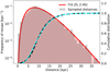 |
Fig. 1. Distance distribution of CNe according to Eqs. (9) and (10) through rejection sampling. Shown are 104 samples (grey histogram, corresponding to a timescale of 200 yr, left axis), and an approximation with the Γ-distribution in red. The cumulative distributions are shown in black for the sample and in cyan for the Γ-distribution (right axis). |
As an alternative to estimating the infinite sum, we calculated the diffuse emission map exactly by line-of-sight integration,
 (11)
(11)
where (x′(s),y′(s),z′(s)) = (xs − scos(l)cos(b),ys − ssin(l)cos(b)), zs − ssin(b)) is the line-of-sight vector starting from the Sun in all directions (l, b) (cf. also Erwin 2015). The total integrated flux of this map is consequently
 (12)
(12)
The intrinsic luminosity of a given density distribution is given by
 (13)
(13)
so that the conversion factor reads
 (14)
(14)
Diffuse quasi-persistent γ-ray emission from the population of CNe in the Milky Way is therefore
 (15)
(15)
In Fig. 2 we show the diffuse emission template and overlay all individual CNe that we considered for this study (Sect. 4). For the two isotopes, the diffuse flux can finally be related to the ejected mass by
 (16)
(16)
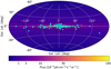 |
Fig. 2. Diffuse emission template from line-of-sight-integrated nova density distribution, Eq. (15), together with nova sample (cyan points). The contours indicate the De Vaucouleurs profile for the bulge and the exponential disc. |
and
 (17)
(17)
where  is the ONe nova rate (Gil-Pons et al. 2003). Using Eqs. (16) and (17) and the theoretical expectations, Sect. 2, we expect a diffuse flux for the 478 keV line of about 10−8–10−5 ph cm−2 s−1. In the energy region of the 7Be decay line, there is strong Galactic background emission, mainly from the ortho-positronium continuum and inverse Compton scattering (e.g., Churazov et al. 2005, 2011; Jean et al. 2006; Bouchet et al. 2010; Siegert et al. 2016, 2019a), which we take into account when the ejected 7Be is calculated in a later step (Sect. 6.2). Even though the expected fluxes for individual objects as well as the diffuse emission of the 478 keV line barely scratch the sensitivity of SPI, a combined fit that takes all objects into account that share similar physics can provide stronger limits on the ejected masses. Likewise, the 1275 keV line from 22Na can be expected to show a diffuse flux of about 10−5–10−4 ph cm−2 s−1. This is well within the sensitivity threshold of SPI. However, the instrumental background line at 1275 keV does not follow the variation of cosmic-ray intensity defined by the solar cycle strictly, but builds up as a function of mission time and thus increases the background at these energies (Diehl et al. 2018).
2.4. Expectations from cumulative signals
From these considerations and theoretical expectations, we compiled a first-order population synthesis model for both isotopes and compared this to the expected background of our chosen data set (see Sect. 3) to obtain a signal-to-noise ratio (S/N). In both cases, we sampled 3D positions according to the combined 3D density distributions, Eqs. (9) and (10), from which distances and Galactic coordinates were calculated. The occurrence of CNe in the Milky Way is a Poisson process (Ross 2008) with a rate of RN ≈ 50 yr−1 for CO novae and  for ONe novae. This means that the waiting time for each CNe after the last one is exponentially distributed. We therefore sampled the waiting times as ΔT ∼ Exp(RN). This provided the explosion date of event n by
  . For the logarithm of ejected masses of ONe novae, we assumed a normal distribution
  and for CO novae
  , presenting conservative estimates from theoretical expectations (Sect. 2.1). The widths of the distributions were chosen to cover the plausible range of theoretical ejecta masses and to not produce unreasonably high γ-ray fluxes that would have already been seen by previous instruments. In a more realistic version of this population synthesis model, the ejecta masses would be distributed according to the mass distribution of WDs on which CNe occur. Because both distributions are fairly uncertain, we considered the general case and only included the range of theoretical models from Starrfield et al. (2009, 2020). Finally, fluxes at the sampled positions were calculated via Eqs. (4) and (5).
We show the characteristic time profile for one realisation in both lines integrated across the whole sky in Fig. 3. Clearly, the flux of the 478 keV line appears more erratic because the lifetime of 7Be is shorter than that of 22Na. Because the lifetime of 7Be is still longer than the average waiting time of about one week, however, the total integrated flux averages to 2–11 × 10−5 ph cm−2 s−1 at any given time. Large peaks, such as around year 18 and 116, are due to individual objects that occurred close to the observer. The diffuse part of the 478 keV emission can be estimated from this to be about 10−5 ph cm−2 s−1, whereas at each given time, the total flux is dominated by about ten individual objects (cf. RNτ7 ≈ 10.5). For 22Na, the decreased ONe nova rate yields a quasi-persistent flux between 4 and 9 × 10⁻⁵ ph cm−2 s−1. In the case of the 1275 keV line, the diffuse flux is dominant, around 5 × 10⁻⁵ ph cm−2 s−1, and individual objects only contribute significantly if they are close to the observer, such as the event in year 116.
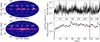 |
Fig. 3. Population synthesis of nova events in a Milky Way-like galaxy. Left: year 116.3 of the modelled Poisson process, where a nearby CO nova at (l, b) = (+123° , + 8° ) outshines the remaining galaxy in 478 keV emission (top). At the same time, 1275 keV emission is not enhanced (bottom). The angular resolution is chosen according to the SPI 2.7° (FWHM). Right: time profiles (light curves) of the 478 keV and 1275 keV since the beginning of the synthesis for a duration of ∼150 yr. This timescale is enough to reach convergence and to show characteristic features. The vertical purple line indicates the time shown in the plots on the left. |
We estimated the range of possible S/N, given these assumptions, using a generic background model (Sect. 5) and 1000 realisations of our CN sample (Sect. 4) and the diffuse emission (Eq. (15)) in Fig. 4 for the case of 22Na. In both cases, individual objects are most of the time below the detection threshold of SPI. However, the cumulative signal of 97 targets that are known to emit at these wavelengths result in an average S/N of ∼5σ for 7Be and ∼3σ for 22Na. In the diffuse-emission case, the 478 keV line would be seen on average with a S/N of ∼1σ and the 1275 keV line with ∼3σ. Therefore both emission lines would show a S/N of ∼5σ when this INTEGRAL data set is considered. However, the allowed range of theoretical ejecta masses leads to considerable uncertainties, being consistent with undetectable signals for SPI even after 16 years. Before the launch of INTEGRAL, Jean et al. (2000) performed a similar study to estimate the chances for SPI to detect the 1275 keV line and suggested that measurements of the diffuse emission could probe ejecta masses ≲10−8 M⊙. Here we show that these pre-launch simulations were too promising.
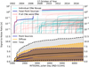 |
Fig. 4. Estimated S/N given the SPI data set (Sect. 3) and the range of plausible 22Na ejecta masses for our sample of 97 novae. Top: the S/N of individual objects does not increase with |

3. SPI data sets
We used publicly available SPI data between 2003 and 2018, including INTEGRAL revolutions 43–1951. Except for a few exceptions, such as V5668 Sgr (Siegert et al. 2018), INTEGRAL did not purposely target CN outbursts, so that the exposure times of our selected sample (see Sect. 4) often contain large gaps or objects are only observed in the partially coded field of view. In a first step, we applied selection criteria based on orbital parameters and instrumental count rates and sensors: Until 2015, we selected orbital phases 0.1–0.9 to avoid the Van Allen radiation belts. Afterwards we only selected orbital phases 0.15–0.85 because of an orbit manoeuvre. We excluded times when the count rate of the SPI anticoincidence shield was increased significantly, for example due to solar flares. We furthermore excluded times when the cooling plate temperatures showed a difference larger than 1 K. Revolutions 1554–1558 were removed from the data set because of the outburst of the microquasar V404 Cygni, which was the brightest soft γ-ray source in the sky during this time. Revolutions in which a detector failure occurred were completely excluded as well.
In a second step, we fit this data set with our instrumental background model and the diffuse emission map (Sect. 5) and removed all pointed observations that showed residuals larger than 10σ. This removed about 0.1% of all selected pointings. We show the resulting exposure map in Fig. 5.
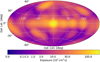 |
Fig. 5. Exposure map of the selected data set. The effective areas around 478 and 1275 keV are ∼80 and ∼55 cm^2, respectively. |
3.1. 7Be
The electron capture of 7Be results in a photon at 477.62 keV from an excited state of 7Li ( ). We used all SPI single events, that is, photons that only interact once with the detector, resulting in 100 105 pointed observations, with a typical exposure time between 1800 and 3600 s. The total dead-time-corrected exposure time, taking failed detectors into account, is 180.1 Ms.
The spectral resolution at 478 keV is about 2.1 keV (Diehl et al. 2018). Additional astrophysical Doppler broadening of the line can be expected from the expansion velocity of the nova ejecta, which typically is in the range of 500–3000 km s−1 (see Sect. 2.1). To include more than 99% of the γ-ray line photons in a single bin for an ejecta velocity of 2000 km s−1, we used an 8 keV wide energy bin between 474 and 482 keV. This includes 7.0 keV broadening due to homologous ejecta, and was added in quadrature to the instrumental resolution.
3.2. 22Na
The decay of 22Na to 22Ne, either through β+ decay ( ) or electron capture, results in a γ-ray photon of 1274.58 keV with
  . At this energy range, electronic noise features in the SPI spectrum can emerge, which can be filtered through pulse shape discrimination (PSD). The selection for PSD events reduces the size of the data set to 99 880 pointings and the exposure time to 179.6 Ms. We note that the fluxes resulting from PSD events have to be re-scaled by an efficiency correction factor ≈1/0.85. The SPI spectral resolution around 1275 keV is about 2.8 keV, so that we performed our analysis in a single 20 keV energy bin between 1265 and 1285 keV to account for possible astrophysical Doppler broadening (as above, Sect. 3.1).
4. Nova sample
4.1. Selecting from databases and catalogues
In order to infer information about the ejecta masses from flux measurements, the distance to the objects and their unambiguous classification as CNe is important. While many astrophysical transients are called ‘novae’, we clearly wished to include only the thermonuclear explosions on the surface of WDs, which are called ‘classical novae’. For current soft γ-ray instrumentation, it is hopeless to detect any CN outside the Milky Way, so that we restricted our selections to our own Galaxy, that is, to objects with galactocentric distances of ≲25 kpc (cf. Fig. 1). This is justified considering the expected quasi-persistent 478 and 1275 keV line fluxes from M31 or the Large Magellanic Cloud (LMC): Using the same formalism from Sect. 2.4 with adjusted CN rates (RN(M31) = 100 yr−1, RN(LMC) = 2 yr−1) and distances (d(M31) = 780 kpc, d(LMC) = 50 kpc), we expect at most 10−7 ph cm−2 s−1 (1275 keV) and 9 × 10⁻⁹ ph cm−2 s−1 (478 keV) from the LMC and 2 × 10⁻⁸ ph cm−2 s−1 (1275 keV) and 2 × 10⁻⁹ ph cm−2 s−1 (478 keV) from M31.
Several comprehensive and well-maintained CN catalogues are available online, but they are scattered in multiple publications and have different information. We first selected CNe from recent peer-reviewed articles, in particular Özdönmez et al. (2018), Shafter (2017), Hounsell et al. (2016, SMEI), Saito et al. (2013, VVV), and Walter et al. (2012, SMARTS). We complemented the information from individual websites that host and update CN lists. These include Koji Mukai’s ‘List of Recent Galactic Novae’ (2008–2020)2, the CBAT ‘List of Novae in the Milky Way’ (seventeenth century until 2010)3, Bill Gray’s ‘List of Galactic Novae’ (‘Project Pluto’; seventeenth century until 2019)4, Christian Buil’s ‘Nova Corner’ (1999–2015)5, and the ARAS Spectral Data Base of Novae (2012–2020)6.
INTEGRAL launched on October 17, 2002 (Winkler et al. 2003), and publicly accessible data are available starting with INTEGRAL revolution 43 (MJD = 52683; February 13, 2003). Owing to the lifetime of 22Na of 3.75 yr, it is also reasonable to include CNe before the launch and first measurements of INTEGRAL. Given the shorter lifetime of 7Be of 0.21 yr and to make a coherent sample, we included all objects from January 1, 2002 (MJD = 52275), to June 30, 2018 (MJD = 58299), that is, 16.5 yr, and those that were at least in the partially coded field of view of SPI (∼30° corner to corner) for 100 ks.
We included all objects whose type was a CN called either ‘fast’, ‘moderately fast’, ‘slow’, or other. This also excluded nova-named objects, such as V838 Mon (Bond et al. 2003) and similarly classified events. The absolute magnitude in UVOIR wavelengths is no selection criterion for this study. We did not include known recurrent CNe in our sample as they would require additional special treatment considering their long-term light curves and ejecta distribution. This further excludes in particular U Sco (the last two known outbursts occurred in 1999 and 2010), RS Oph (1985 and 2006), and IM Nor (1920 and 2002).
In total, this provides a sample of known objects within the considered time frame of 97 CNe. Given the CN rate of ∼50 yr−1, about ∼12% of all expected objects are included as point sources with known positions in this study (Sect. 2.2). The remaining ∼88% of unknown sources plus hundreds of CNe from before the start of the considered time frame then make up the diffuse component of the γ-ray emission (Sect. 2.3). The full list of objects can be found in Table B.1.
4.2. Handling unknown distances
For 44 CNe in this sample – mainly older objects –, a distance estimate is available from the different input catalogues and websites. When two or more estimates were available for one object, we used the most recent value. Most of the distance estimates for CNe come from the maximum magnitude relation with decline time (MMRD, Zwicky 1936; McLaughlin 1940; Buscombe & de Vaucouleurs 1955). For objects located inside a certain cluster or galaxy, this method provides reliable estimates for the population distance. However, individual CNe inside the Milky Way still carry uncertainties on their distances of about 30–50%. For example, the distance estimate of 3 ± 1 kpc for V5115 Sgr (Table B.1) would suggest an ejecta mass uncertainty of at least 66% (≈0.2 dex), ignoring the flux uncertainties.
The problem of converting estimated fluxes into ejecta masses for objects with unknown distance is even more severe: When we consider the distance distribution of CNe inside the Milky Way from the point of Earth, Fig. 1, it is clear that most sources are expected around the Galactic centre. However, an object found toward the Galactic anticentre with unknown distance will most certainly not be at such a large distance; these distances are still possible, but only with a probability P(7 < d < 9) ≈ 17%. Very UVOIR-bright CNe could be located close to Earth, but with an unavailable distance estimate: The probability that any object is located inside a sphere of radius 0.5 kpc (1.0 kpc) is P(d ≤ 0.5) ≈ 3 × 10⁻⁵ (5 × 10⁻⁴). Given the CN rate, less than one object is expected within these distances during the INTEGRAL observations, consistent with no γ-ray detection so far. These considerations make the distribution in Fig. 1 and its approximation with dunknown ∼ Γ(αd = 4.25, 1/βd = 1/2.45) a reasonable first-order distance estimator for any CNe inside the Milky Way, independent of its direction as seen from Earth. We use the approximated distribution as prior information for inference in Sect. 5.2.1 to construct a full posterior for the ejecta masses that properly takes all uncertainties into account.
We estimated the effect of using this generic distribution by naive scaling factors as above: As described in Sect. 2.3, the expectation value of distances is ⟨dunknown⟩ = 10.4 kpc, with a standard deviation σdunknown = 5.1 kpc. Half of all CNe observed from Earth are found within a sphere of 9.6 kpc, thus including the Galactic bulge, nearby high-latitude objects, and the Galactic anticentre, and thus also covering most known CN distances (Table B.1). When we consider the symmetric 90% interval around the expectation value, a canonical distance uncertainty of 7.6 kpc can be given. This makes the ejecta masses of objects with unknown distances uncertain by at least 150% (≈0.4 dex). Given the large total volume of the Milky Way, this appears as a reasonable estimate.
5. SPI data analysis
5.1. General method
The SPI data djpe are detector (j) triggers per unit time (pointing p) and energy (e), and consequently follow the Poisson distribution,
 (18)
(18)
where mjpe is the (modelled) rate parameter. In our analysis, the energy is fixed and we omit the index e in the following. The likelihood of measuring djp counts in the selected data set D, given a model M with expectation mjp, is
 (19)
(19)
We modelled the SPI counts as a linear combination of sky components and background models,
 (20)
(20)
In Eq. (20), NN is the number of CNe in our sample, plus one model component to account for diffuse emission. Fi, p is the flux of sky model Si, lb to which the imaging response function  was applied (mask coding). The background model Bk, jp was split into two components, k = L and C, accounting for instrumental line and continuum background, respectively. Temporal variations in the background were determined by the parameters βk, scaling the amplitudes of the two components (cf. Siegert et al. 2019b). The expected flux of point-like sources (individual CNe) was determined according to Eqs. (4) and (5). Because the exponential decay times are known, the pointing-to-pointing variation can be fixed in Eq. (20), and only one parameter was fitted for each source and isotope. The expected diffuse flux was modelled according to Eqs. (16) and (17). In the individual CN case, the spatial model is one point at the coordinates of the CN. For diffuse emission, the flux is constant in time and distributed according to the line-of-sight-integrated density structure Eq. (15). Finally, the fit parameters of interest are the maximum flux F at the time of explosion T0, which can be split into a function of ejecta mass Mej and distance d for point sources, and mass and CN rate RN for diffuse emission.
Clearly, this would result in an ill-defined likelihood function if the distances and the CN rate are not constrained. In the case of a known distance for CNe in our sample, we incorporated a normal prior on the distance. When the distance to an object was not known, we used the information that the CN occurred inside the Milky Way, which translates into a distance prior according to a Γ-distribution dunknown ∼ Γ(αd = 4.25, βd = 1/2.45) (see Sects. 2.3 and 4.2). This sets any object for which the distance is unknown on average to αd/βd = 10.4 kpc with a standard deviation  kpc (cf. Fig. 1). For the CN rate, we set a prior according to the most recent literature value in units of yr−1 of RN ∼ 𝒩+(50, 252) (index +: truncated at zero) for all CN types and
  for ONe novae (Shafter 2017). Especially the prior for the CN rate is particularly broad and can, in principle, be consistent with zero. A zero rate, however, is unphysical because CNe constantly occur throughout the year. We nevertheless included this extreme to show a broad range for the remaining parameter space. We set a uniform prior on the logarithm of the ejecta mass, lgMej ∼ 𝒰(−11, −4), so that each decade considered in the parameter space obtained the same prior probability, and a wide range of theoretical and otherwise plausible values were sampled. The lower bound on the ejecta mass prior of 10−11 M⊙ is data driven, as above considerations (Sect. 2.4) show that SPI is incapable of probing these values except for distances smaller than 100 pc.
Details on the background modelling procedure can be found in Diehl et al. (2018) and Siegert et al. (2019b). In short, the background is modelled by long-term monitoring of the complete SPI spectrum and the spectral response changes. This results in a background and response database per INTEGRAL orbit and detector for several 100 background lines, and the underlying continuum. Because the background dominates the measured count rate at any time, and in addition, the coded mask pattern from celestial objects smears out on a timescale of tens of pointings (typically 50–100 in one INTEGRAL orbit), a background response can be constructed from this database. The short-term pointing-to-pointing variation is fixed by an onboard counting rate, in our case, the saturating germanium detector events. Finally, any variation that is not captured by this procedure is handled by the introduction of the background re-scaling parameters βk. In both cases, we find that one parameter per INTEGRAL orbit per background component is enough to provide an adequate fit. The total number of fitted parameters for one object finally is twice the number of INTEGRAL orbits, plus two for the flux, that is, npar = 2 ⋅ 1674 + 2 = 3350. For the 478 keV line (1275 keV), the number of data points excluding dead detectors is 1598964 (1595430).
5.2. Hierarchical modelling approach
In order to combine the extracted posterior distributions of the flux, we applied a hierarchical model (Gelman et al. 2013) in three different steps. In Fig. 6 we show the full graphical model as separated into interesting parameters, nuisance parameters, fixed parameters, resulting spatio-temporal models, and their interdependencies. When we consider the sky emission from top to bottom, the hierarchy flows from superordinate hyper-parameters μ and τ, which describe the distribution of ejecta masses Mi of each CN i, which then determines the fluxes, given additional parameters: Depending on the distances di, or in the diffuse case, the CN rate RN, absolute fluxes Fi and Fdiff result from Eqs. (4), (5), (16), and (17). These are either point-like at source positions (l, b)i or distributed according to the line-of-sight integration of ρ (cf. Eqs. (9), (10), and (15)), resembling the sky models  and
and  , respectively. For individual objects, the discovery times T0, i are known7, after which the flux is exponentially decaying according to isotope-specific parameters (Eq. 1). The diffuse emission component is constant in time. In particular, this scheme is included in our Poisson process, Sect. 2.4. We now try to infer the values of Mi and/or μ and τ.
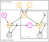 |
Fig. 6. Complete graph of different model variants used in this study. When the source models are used individually, that is, regardless of a common underlying physical process, the most conservative estimates are found in a no pooling setting (Sect. 5.2.1). The opposite extreme assumes that all objects eject the same amount of matter, so that instead of ∼100 different masses, only one is fitted. This resembles complete pooling and defines tight constraints but is subject to bias if the true variance is large (Sect. 5.2.2). A compromise between no and complete pooling is achieved by invoking the hyper-parameters μ and τ that determine the mean and the spread of ejecta masses, if any (partial pooling, dash-dotted box, Sect. 5.2.3). |
Ideally, all sky models are convolved with the imaging response to convert them into a SPI-compatible format and are then fitted simultaneously to the raw SPI count data, together with the two-component background model. Given the large number of data points, fitted parameters, and especially their interdependence in the full hierarchy (see Sects. 5.2.1–5.2.3), this is computationally very expensive and not feasible without very many high-performance computing hours. Instead, we applied the hierarchical model in a two-step process:
First, we extracted the fluxes of each of the NN = 97 CNe and the diffuse emission individually (Eq. (20)). This resulted in posterior distributions for the fluxes of all sky models considered. To first order, these posteriors follow a Γ-distribution8, so that instead of the previous 1.5 million data points, we condensed the information into the two shape parameters, α and 1/β of the Γ-distribution for each sky model. Thus, in a second step, we applied the hierarchical model to a reduced data set consisting of (97 + 1) ⋅ 2 shape parameters.
Because the actual measurement information (Poisson counts) is lost in this procedure, the resulting combined values are approximations to the true distribution. We already note here that none of the sources considered show a significance above background of more than 2.5σ, so that most flux posteriors are sharply peaked at zero flux, with a long tail according to the Γ-distribution.
5.2.1. No pooling
The most agnostic view about the physics at play is provided by treating each object individually (no pooling). This means that we let the data speak for themselves if uninformative or weakly informative priors are used, as is the case for our general method: The flux extraction step, Sect. 5.1, is equivalent to a no pooling analysis. Because we are interested in the ejecta masses, we fit the two shape parameter of the flux posteriors, in particular their expectation values ⟨Fi⟩=αi/βi, according to the likelihood
 (21)
(21)
where  are the latent fluxes according to Eqs. (4), (5), (16), and (17). By definition, this results in a distribution for the flux of each object that is consistent with the input distribution and an expectation value
  . By adding the distance (or CN rate) information in a prior, we obtain the posterior distribution of ejecta masses for each individual object (and diffuse emission) independently, according to the measured flux and its asymmetric uncertainties. This determines 98 values for
  from 98 data points and their 98 uncertainties. For completeness, we repeat the prior probabilities that are used here and elsewhere in the paper for the same parameters:
 (22)
(22)
with μd and σd from Table B.1 in units of kpc, αd = 4.25 and βd = 1/2.45 such that αd/βd = 10.4 kpc is the expectation value of CNe with unknown distances,  and
and  , μRN = 50 yr−1 and σRN = 25 yr−1, and
  and
and  . Instead of using truncated normal distributions for the event rates, we also tested log-normal distributions with the same means and variances for the hierarchical model fits. This avoids the unphysical boundary of a (nearly) zero rate. The posterior distribution of the ejecta masses in each object, marginalised over the nuisance parameters distance and rate, finally reads
 (23)
(23)
In Eq. (23), P(Mej, d, R) is the joint prior distribution, built as multiplicative distribution from Eq. (22).
We note that neither the true Poisson count data nor the condensed data set can constrain the distance (or rate) information, which consequently is only a nuisance parameter and included to properly convert the flux values into ejecta masses, given the uncertainties on the distances (or rate). Of our 97 objects, certainly not all are ONe novae. Nevertheless, we determined the upper bounds for the 1275 keV line flux and the resulting 22Na ejecta mass bounds from these objects. A more detailed discussion of the results and limits from individual objects is presented in Sect. 6.1. The complete results table can be found in Table B.1.
5.2.2. Complete pooling
One way to improve upon estimates from individual objects – which in our case are rarely constraining (Sect. 6.1) – is to include the whole population and assume that each object (and the cumulative diffuse emission) stems from the same ejected mass. When we consider Fig. 6, this means that  , and the resulting fluxes ⟨F⟩i (and ⟨F⟩diff) share a common dependence in the complete pooling setting. This is sometimes called ‘stacking’ (e.g., Malz 2021), which is not equivalent in detail, however, because the extracted spectra (or fluxes) are not stacked to obtain an average spectrum, but the model parameters are shared among all objects. For a completely pooled (combined) posterior for the ejected mass, we thus sampled the fluxes according to the likelihood
 (24)
(24)
The only difference between Eqs. (24) and (21) is that there is only one parameter of interest,  , which is then representative for the whole population. This determines one value for Mej from 98 data points and their 98 uncertainties, which are dependent on each other, and it still includes all uncertainties from distances, rates, and individual flux measurements.
Complete pooling results in the most optimistic but also most biased estimate of the ejecta masses. Because the known effects of different ejecta masses for different WD masses and compositions are ignored in this setting, the resulting estimate is equivalent to the mean of the population of CNe. This mean is not necessarily a useful number because it is dominated by the most abundant objects, most frequent CN types, or observations with the smallest uncertainties.
5.2.3. Partial pooling
Because of the different astrophysical and measurement-related effects, the true ejecta masses of CNe in the Milky Way may follow a distribution that can be described by a mean value μ and a width τ, such that
 (25)
(25)
This means that we first sampled ejecta masses according to the distribution, Eq. (25), and then again sampled the flux distributions as before, but now the distributions depended on the hyper-parameters μ and τ rather than  individually. The likelihood becomes
 (26)
(26)
This partial pooling setting is a compromise between no pooling and complete pooling: depending on the value of τ, the samples of ⟨Fi⟩ either converge to one common value (complete pooling, τ → 0) or spread out towards their independent values (no pooling, τ → ∞). The prior for the mean of this hyper-distribution was chosen similar to that of the individual masses, μ ∼ 𝒰(−11, −4). The prior for the width τ is discussed in the literature (Gelman et al. 2013, and references therein), depending on the purpose of the analysis. We tested two priors for τ: first, a uniform distribution between 0 and 10, which is agnostic about the fact that each object should indeed rather be similar in ejecta mass and should not show a difference of several orders of magnitude. However, especially in the case of the 1275 keV emission, such a prior would be useful because the ejecta masses would indeed be either close to zero (CO novae) or around a certain mean (ONe novae). Second, we tested a half-Cauchy prior for τ with width 1. This assumes that most objects follow a similar trend, but also allows for a broader distribution that might include several outliers.
We note that our data are mostly dominated by the measurement uncertainties so that the choice of the prior for τ has no effect on the result, and both converge around the same point (Sect. 6.3). Partial pooling determines the two shape parameters of the ejecta mass distribution, Eq. (25). The upper bounds of μ can then be interpreted as conservative upper bounds on the ejecta masses of 7Be and 22Na in individual CN events in the Milky Way, taking into account the complete population and its uncertainties from the SPI measurements.
6. Results
6.1. Individual objects
In Fig. 7 we illustrate the bounds on the 22Na ejecta masses for each object at its (un)known distance, and how the estimates relate to upper bounds on the flux. All our upper bounds are quoted on the 99.85th percentile level if not mentioned otherwise. Apparently bright objects for which the flux is not consistent with zero within 2σ, the full posterior distributions are shown (here only V1535 Sco). Clearly, the mass estimates are inherently bound by the observation time towards the target and the exponential decay law winning over the square-root of time increase in sensitivity. Even though several objects have been frequently re-visited since the beginning of the INTEGRAL mission, all become saturated in terms of significance above background. This leads to an apparently common upper bound of the fluxes between 3 × 10⁻⁵ and 3 × 10⁻⁴ ph cm−2 s−1 for 22Na and 10−4 to 3 × 10⁻³ ph cm−2 s−1 for 7Be (see Fig. A.1), which cannot be improved on the individual object basis. Only a nearby ONe nova (≲1.0 kpc) or one with exceptionally high ejecta mass would be seen with INTEGRAL/SPI. The remaining variance in flux bounds and hence ejecta mass bounds stems from the varying background level in this 16-year data set, as well as on exposure differences.
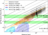 |
Fig. 7. Summary of the no pooling analysis. Shown are the upper bounds (99.85th perc.) on the ejecta mass of 22Na for each object with known (orange) and unknown (black) distance. The dependence on distance lets the bounds on mass appear along the lines of constant flux (dashed lines). Full posteriors are given for objects with the best flux bound (V5115 Sgr), the best mass bound (V5113 Sgr), and whenever the significance is higher than 2σ (V1535 Sco). Theoretical expectations (Starrfield et al. 2009) are indicated by the green bands for 1.25 and 1.35 M⊙ ONe novae. Other theoretical expectations are bound to values below ≈ 10−8 M⊙ (e.g., José & Hernanz 1998). See text for a discussion of individual objects. |
Nova V1535 Sco shows the highest significance above instrumental background with 2.5σ. With a distance of 5.3 ± 1.7 kpc, this would be an unexpectedly high 22Na ejecta mass. Furthermore, it is not known whether V1535 Sco is an ONe or CO nova. Hard X-ray emission (> 1 keV) has been found in V1535 Sco within a few weeks after its discovery on February 11, 2015, with a peculiar behaviour that is thought to be an indication of the CN being embedded in a red giant star (Linford et al. 2017). V1535 shows no to weak indications of GeV emission (Franckowiak et al. 2018), probably because of its large distance. We find this enhanced S/N only for the 1275 keV line, which would be unexpected if the emission was due to a CN outburst.
In our sample, we obtain the lowest upper bound on the 1275 keV line flux for V5115 Sgr. The large exposure toward the Galactic centre (cf. Fig. 5) and its outburst time on March 28, 2005 (Nakano et al. 2005), leads to an upper bound on the 1275 keV line flux of < 3.6 × 10⁻⁵ ph cm−2 s−1. V5115 Sgr is probably an ONe nova with a WD mass of 1.2 ± 0.1 M⊙ (Hachisu & Kato 2006; Shara et al. 2018). At a distance of 2.8 ± 1.0 kpc, the upper bound on the flux converts into an upper bound on the 22Na ejecta mass of < 1.3 × 10⁻⁷ M⊙. This excludes WD masses around 1.3 M⊙ (see Fig. 7), fully consistent with theoretical expectations (Starrfield et al. 2009) and independent measurements (Hachisu & Kato 2006). Using this bound, we can set a lower bound on the distance of V5115 Sgr of ≳2.0 kpc because otherwise, SPI would have seen the 1275 keV line. We note again that longer exposures for this object will not result in any improvements on the flux or ejecta mass because most 22Na has already decayed.
We obtain the tightest limit on the 22Na ejecta mass for the object closest to us, as expected, here V5113 Sgr with a distance estimate of 0.9 ± 0.2 kpc. At this distance, we infer a bound on the mass up to < 2 × 10⁻⁸ M⊙. If V5113 Sgr was an ONe nova, this would set tight constraints on the nucleosynthesis on such objects, as it would fall below the lowest theoretical estimates (e.g., Starrfield et al. 2009). There are no indications that V5113 Sgr is indeed an ONe nova (Tanaka et al. 2011; Mróz et al. 2015), nor is the mass of the WD constrained.
We note that the mass estimates for 7Be and 478 keV are one to two orders of magnitude above theoretical expectations in most cases. We refer to Appendix A for these results.
6.2. Diffuse emission
In Fig. 8 we show the posterior distribution of the diffuse 1275 keV line flux in the Galaxy, accounting for possible continuum emission, and separated into ONe nova rate and 22Na ejecta mass. The illustrated flux posterior takes into account that a weak diffuse Galactic continuum emission is present in the band 1265–1285 keV. We determined the total flux in this band according to  , where
  in units of 10−5 ph cm−2 s−1 (Wang et al. 2020). From this, we find an upper bound on the diffuse 1275 keV line flux of < 3.9 × 10⁻⁴ ph cm−2 s−1 in the entire Galaxy, which converts into an upper bound on the 22Na ejecta mass of < 2.7 × 10⁻⁷ M⊙. We wish to point out that this value is similar to the one found by Jean et al. (2001) with COMPTEL (< 3 × 10⁻⁷ M⊙), which only focused on the inner Galactic ridge (|l|< 30°). Our analysis takes the uncertainties on the ONe nova rate, the asymmetric flux estimate from the SPI count data, as well as possible continuum contribution into account, whereas the analysis by Jean et al. (2001) considered different spatial distributions for CNe.
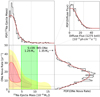 |
Fig. 8. Posterior distributions for diffuse emission of the 1275 keV line. The flux (top right) is separated into its two determining components, the 22Na ejecta mass (top left) and the ONe nova rate (bottom right, treated as a nuisance parameter). Theoretical predictions are indicated in green from Starrfield et al. (2009). The joint posterior (68.3th, 95.4th, and 99.7th percentile) of ejecta mass and nova rate (bottom left) shows the expected anticorrelated behaviour according to Eq. (17). |
The energy band 474–482 keV is detected with more than 11σ above instrumental background with a flux of  . Most of this flux originates in the three-photon decay of ortho-Positronium in the interstellar medium, plus small contributions from inverse Compton scattering and unresolved high-energy sources for an integrated continuum flux of
  (e.g., Strong et al. 2005; Bouchet et al. 2011; Siegert et al. 2016). When we take this into account, we obtain an upper bound on the diffuse 478 keV line flux of < 5.9 × 10⁻⁴ ph cm−2 s−1, which converts into a 7Be ejecta mass of < 4.1 × 10⁻⁷ M⊙. Again, the 7Be values are not constraining, and we refer to Appendix A for the results of the 478 keV line.
6.3. Combined analysis
Because none of the objects are individually detected, the hierarchical analysis mainly takes into account the asymmetric uncertainties on these flux measurements. This allows us to define common (population) upper bounds on the ejecta mass, given the individual uncertainties from fits to the SPI raw count data.
In Fig. 9 we show the summary of our hierarchical model for the 22Na case. As τ goes to zero in the case of complete pooling, all values (here: upper bounds on the ejecta mass) converge to one single point,  . This assumes that the ejecta mass of all individual point sources in our CN sample and the diffuse emission to originate from the same 22Na ejecta mass. We know that this is not the case (see Sect. 6.1), and we describe two ways of lifting these restrictions below.
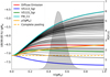 |
Fig. 9. Summary of the hierarchical model. Shown are the upper bounds on the 22Na ejecta masses (left axis) for individual objects (black) as a function of the population width τ, together with the complete pooling estimate (τ → 0, dashed orange), and the population mean μ (solid orange). Individual objects of interest (best (blue) worst (aqua) bound, diffuse emission (red)) are indicated. As τ → ∞, each upper bound converges to its no pooling value (Table B.1). Given the SPI flux posteriors, a population width of |

In an attempt to account for the fraction of 1/3 of all CNe to be ONe novae, we used a finite mixture model with exactly this defined ratio RCO : RONe = 2 : 1 and repeated the CP analysis. This mixture model selected a sub-sample of one-third of our sample and fitted it according to Eq. (24), whereas the remaining sample was subject to a prior distribution for the ejecta mass according to CO novae ( , Starrfield et al. 2020), resulting in basically zero flux for every object. The fit resulted in an increased upper bound of
  .
.
Alternatively, we used the partial pooling approach (Sect. 5.2.3) and inferred the upper bound on the population ejecta mass by determining the spread τ of the distribution of ejecta masses. Ideally, τ would be determined by a combination of the true spread of the ejecta from many observations and their inherent uncertainties. Here, τ is almost purely defined by the measurement uncertainties of the asymmetric flux posteriors. We find that independent of the choice on the prior of τ (cf. Sect. 5.2.3), its posterior populates the range  (C.I. 99.7%) with a population mean μ22 < 2.0 × 10⁻⁷ M⊙. This means that the broadest allowed ejecta mass distribution of the population of 22Na-ejecting CNe that would still be consistent with our data is
  . In other words, if the mean of the ejecta mass distribution were any higher than 2 × 10⁻⁷ M⊙, one or more objects (or the diffuse emission) would have been seen by SPI with at least 3σ above the instrumental background. This value is higher than the tightest constraint from V5113 Sgr in the no pooling context (
 as τ → ∞ and assuming V5113 Sgr is an ONe nova; cf. Table B.1), for example, but smaller than the one purely from diffuse emission. This can be considered the most conservative upper bound on the 22Na ejecta mass from ONe novae because 1) it does not restrict high ejecta masses as would be case in the complete pooling setting, 2) it takes the diffuse emission and known explosions into account, and 3) it considers the entire Galaxy. Using a log-normal prior for the rate decreases the upper bound on the population mean by less than 5%.
While the rate has only a marginal effect on the final population estimate, the non-detection of individual sources also suppresses the diffuse emission flux and hence lowers the ONe rate: The initial prior mean was  with a standard deviation of
  . Now, the posterior mean of μRONe is found at 6 (complete pooling) and 13 yr−1 (partial pooling), with a standard deviation of 3 and 7 yr−1, respectively, independent of the prior shape. If all CNe happen to eject the same small amount of 22Na as given in the complete pooling setting, the ONe nova rate in the Milky Way would be 18 yr−1 at most (99.85th percentile). Clearly, this assumption is extreme and the more conservative upper bound on the ONe nova rate from partial pooling is 40 yr−1, also independent of the prior shape.
In the case of 7Be and the 478 keV line, the shape of Fig. 9 is almost identical, only the numbers are spread further. We find an upper bound on the 7Be ejecta mass from complete pooling of  and from partial pooling of μ7 < 2.5 × 10⁻⁷ M⊙. Neither of these values is constraining compared to theoretical expectations, which predict at most 4 × 10⁻¹⁰ M⊙ (e.g., Starrfield et al. 2009). However, individual CNe have been found with a higher 7Be ejecta mass, of about several 10−9 M⊙ (e.g., Molaro et al. 2016; Tajitsu et al. 2016, 2015), which indeed suggests a larger spread in ejecta masses than what is currently discussed.
7. Discussion
7.1. Nova nucleosynthesis
All our upper bounds are consistent with theoretical expectations. Considering the lowest theoretical expectations for 1.35 M⊙ WDs from Starrfield et al. (2009), for example, of ≈ 3.9 × 10⁻⁷ M⊙, we find 18 objects whose upper bounds on the ejecta mass would be below this threshold. These 18 objects include V5115 Sgr and V5113 Sgr, which we mentioned above (Sect. 6.1). We find that 9 objects are probably CO novae, 3 are probably ONe novae, and 6 are not determined. Considering the three ONe novae V5115 Sgr, V382 Nor, and V1187 Sco and our ejecta mass estimates ( ,
,  ,
,  ; cf. Table B.1), we find that these events occurred on WDs with masses lower than 1.35 M⊙. This is fully consistent with the independent WD mass estimates from Shara et al. (2018). In general, our upper bounds can be interpreted to mean that most ONe novae in the Milky Way occur on WDs with masses lower than 1.35 M⊙ because otherwise, SPI would have seen a stronger signal. This is expected because the mass distribution of measured WDs in the Galaxy peaks around 1.13 M⊙ with a width of 0.12 M⊙ (Shara et al. 2018). Other theoretical models predict lower 22Na yields of about 10−8 M⊙ (e.g., José & Hernanz 1998). When these models are considered, our results cannot provide any constraints.
The upper bound on the 22Na ejecta mass from ONe novae translates into a steady-state 22Na production of 3.3 × 10⁻⁶ M⊙ yr−1. On a timescale of 10 Gyr, ONe novae hence produced 3.3 × 10⁴ M⊙ of 22Ne at most, assuming the ONe nova rate is constant. With the solar abundance ratios by Lodders (2003), the Galaxy would contain a 22Ne mass of ≈7.5 × 10⁴ M⊙. Clearly, a full population synthesis model would be required to compare the upper bound on the 22Ne mass from CNe with the total Galactic content. We nevertheless provide these order-of-magnitude evaluations to show a general broad consistency.
While the results from 7Be are far from constraining, we can provide a similar upper bound on the total 7Li mass inside the Milky Way. With the upper bound on the 7Be ejecta mass from the population of CNe of  , we find that on a timescale of 10 Gyr, 1.25 × 10⁵ M⊙ of 7Li has been produced at most. This is about two to three orders of magnitude above the theoretical values from Starrfield et al. (2020), who suggested that about 100 M⊙ of the 1000 M⊙ of 7Li in the Milky Way is due to CO novae. To further constrain the 7Li production in the Milky Way from CNe with soft γ-rays, an instrument with a sensitivity improvement by two orders of magnitude would be required (see also next Section).
7.2. Positrons from classical novae
Given the upper bound on the 22Na ejecta mass from ONe novae in the Milky Way of  , we can estimate how much CNe contribute at most to the Galactic positron budget. With the probability of 22Na to decay through β+ decay of
  , the production rate of positrons from the population of ONe novae is
 (27)
(27)
Siegert et al. (2016) estimated a total positron annihilation rate in the Milky Way of Re+ ≈ 5 × 1043 e+ s−1. Assuming a steady-state annihilation in the Galaxy, this rate has to be sustained by the same production rate. The population of ONe would therefore contribute 10% at most to the total Galactic positron production rate. This is of similar magnitude as other known and validated source types, such as 26Al from massive stars and their supernovae (≈10%; τ26 = 1.05 Myr) and 44Ti from core-collapse supernovae (≈10%; τ44 = 86 yr). For the remaining 80% required for steady-state annihilation, several other individual source types, populations, and scenarios have been suggested. However, only indirect evidence for positron annihilation and production in these sources has been found so far (cf. Prantzos et al. 2011, for a review).
The population of CNe in the Galaxy will have a small but important contribution to the total positron production rate, complementing the different nucleosynthesis origins of Galactic positrons with frequent occurrences of CNe and comparably short lifetimes of parent nuclei. These considerations do not exclude the very short-lived light β+-unstable nuclei 13N or 18F from contributing significantly to the total content. Because the expected very strong 511 keV flash at the time of the explosion has never been observed, it might even be possible that these positrons also do not annihilate in the expanding nova cloud, but rather escape into the interstellar medium. This would make CNe a dominant source of positrons in the Milky Way.
Theoretical modelling of nucleosynthesis yields predicts values close to our upper bounds. This suggests a bright future for the next generation of soft γ-ray telescopes such as COSI (Tomsick et al. 2019) in nuclear decay and the 511 keV positron annihilation line.
8. Conclusion
We used 15 years of archival INTEGRAL/SPI γ-ray observations to infer nucleosynthesis ejecta masses of decaying 22Na and 7Be from the population of classical novae. In our sample of 97 individual known objects, no signal is detected above a threshold of 3σ.
The best upper bound for an individual CO nova is found for V5668 Sgr owing to a dedicated observation campaign (see Siegert et al. 2018), with a 478 keV line flux of < 1.4 × 10⁻⁴ ph cm−2 s−1, resulting in a 7Be mass of < 3 × 10⁻⁸ M⊙. For the first time, we considered the diffuse 478 keV line component of CO novae in the Milky Way and found an upper flux bound of < 6.0 × 10⁻⁴ ph cm−2 s−1, which converts into an average ejecta mass of < 4.1 × 10⁻⁷ M⊙. We improved these values by using a Bayesian hierarchical model of 478 keV emitting novae, that is, we took a common distribution of ejecta masses into account and inferred a population mean of < 0.5– 2.5 × 10⁻⁷ M⊙. While these values are hardly constraining compared to theoretical expectations (e.g., Starrfield et al. 2020), we nevertheless showed that proper modelling of sub-threshold sources can provide a significant improvement on the pure stacking of many point sources.
For individual ONe novae, our most constraining upper bounds on the 22Na ejecta mass are found for V5115 Sgr and V1187 Sco with < 1.3 × 10⁻⁷ M⊙. The lowest 1275 keV line upper bound is found for V2659 Cyg with < 2.9 × 10⁻⁵ ph cm−2 s−1, but at an unknown distance. The expected diffuse emission of the 1275 keV line in the Milky Way along the Galactic plane with a strong peak in the bulge provides an upper flux bound of < 3.9 × 10⁻⁴ ph cm−2 s−1, which converts into a 22Na ejecta mass bound of < 2.7 × 10⁻⁷ M⊙. Our Bayesian hierarchical model for the 1275 keV line results in a population mean of < 0.7–2.0 × 10⁻⁷ M⊙. These values are an improvement over previous studies: (1) the upper bounds on the ejecta masses are 2–5 (depending on the model assumptions) times smaller than from earlier COMPTEL measurements (Jean et al. 2001), and (2) they take into account both diffuse emission and known sources, their individual uncertainties, and uncertainties on circumstantial parameters, such as the nova rate and distances.
The result can be interpreted in a way that if the population mean of ejecta masses were any higher, one or more ONe novae would have been detected with at least 3σ by INTEGRAL/SPI in this 15 yr data set. Still, these upper bounds are on the high side of theoretical expectations (e.g., Starrfield et al. 2009): We can exclude that most ONe novae occur on WDs with masses of about 1.35 M⊙, and thus finally probe the region of model calculations. When we tighten the uncertainties on nova rate and individual distances, for example, and at the same time might make use of the full data set rather than relying on extracted fluxes, the hierarchical model would probably probe even deeper, that is, set tighter bounds on ejecta masses.
With 22Na as a β+ decayer, we find an upper bound on the positron production rate in the Milky Way from ONe novae of < 5.5 × 1042 e+ s−1. Compared to the Galactic positron annihilation rate (Siegert et al. 2016), the population of ONe could make up to 10% of the required positron production rate for a steady-state configuration.
The explosion times are expected 2–10 days before the discovery (Gomez-Gomar et al. 1998). This defines our systematic uncertainties in the case of CO novae of exp(0.1) ≈ 10% and ONe novae of exp(0.005) ≈ 0.5% and is much smaller than the statistical uncertainties.
In particular, the posterior of a Poisson rate is exactly Γ-distributed if the conjugate prior for the Poisson distribution is used, the Γ-distribution (Gelman et al. 2013).
Acknowledgments
Thomas Siegert is supported by the German Research Foundation (DFG-Forschungsstipendium SI 2502/1-1 & SI 2502/3-1). He thanks J. Michael Burgess for suggesting to do something important. This work used the Extreme Science and Engineering Discovery Environment (XSEDE), which is supported by National Science Foundation grant number ACI-1548562. We acknowledge the use of XSEDE resources via Startup allocation TG-PHY200045. Software: OSA/spimodfit (Halloin 2009), numpy (Oliphant 2006), matplotlib (Hunter 2007), astropy (Astropy Collaboration 2013), scipy (Virtanen et al. 2020), Stan/pystan (Carpenter et al. 2017), arviz (Kumar et al. 2019).
References
- Astropy Collaboration (Robitaille, T. P., et al.) 2013, A&A, 558, A33 [NASA ADS] [CrossRef] [EDP Sciences] [Google Scholar]
- Bond, H. E., Henden, A., Levay, Z. G., et al. 2003, Nature, 422, 405 [Google Scholar]
- Bouchet, L., Roques, J. P., & Jourdain, E. 2010, ApJ, 720, 1772 [NASA ADS] [CrossRef] [Google Scholar]
- Bouchet, L., Strong, A. W., Porter, T. A., et al. 2011, ApJ, 739, 29 [NASA ADS] [CrossRef] [Google Scholar]
- Bouchet, L., Jourdain, E., & Roques, J.-P. 2015, ApJ, 801, 142 [NASA ADS] [CrossRef] [Google Scholar]
- Buscombe, W., & de Vaucouleurs, G. 1955, Observatory, 75, 170 [NASA ADS] [Google Scholar]
- Carpenter, B., Gelman, A., Hoffman, M. D., et al. 2017, J. Stat. Software, 76, 1 [CrossRef] [Google Scholar]
- Churazov, E., Sunyaev, R., Sazonov, S., Revnivtsev, M., & Varshalovich, D. 2005, MNRAS, 357, 1377 [NASA ADS] [CrossRef] [Google Scholar]
- Churazov, E., Sazonov, S., Tsygankov, S., Sunyaev, R., & Varshalovich, D. 2011, MNRAS, 411, 1727 [NASA ADS] [CrossRef] [Google Scholar]
- Clayton, D. D. 1981, ApJ, 244, L97 [CrossRef] [Google Scholar]
- Clayton, D. D., & Hoyle, F. 1974, ApJ, 187, L101 [NASA ADS] [CrossRef] [Google Scholar]
- Diehl, R., Halloin, H., Kretschmer, K., et al. 2006, Nature, 439, 45 [NASA ADS] [CrossRef] [PubMed] [Google Scholar]
- Diehl, R., Siegert, T., Greiner, J., et al. 2018, A&A, 611, A12 [NASA ADS] [CrossRef] [EDP Sciences] [Google Scholar]
- Erwin, P. 2015, ApJ, 799, 226 [Google Scholar]
- Franckowiak, A., Jean, P., Wood, M., Cheung, C. C., & Buson, S. 2018, A&A, 609, A120 [NASA ADS] [CrossRef] [EDP Sciences] [Google Scholar]
- Gelman, A., Carlin, J. B., Stern, H. S., et al. 2013, Bayesian Data Analysis, 3rd edn. (CRC Press) [Google Scholar]
- Gil-Pons, P., García-Berro, E., José, J., Hernanz, M., & Truran, J. W. 2003, A&A, 407, 1021 [NASA ADS] [CrossRef] [EDP Sciences] [Google Scholar]
- Gomez-Gomar, J., Hernanz, M., José, J., & Isern, J. 1998, MNRAS, 296, 913 [NASA ADS] [CrossRef] [Google Scholar]
- Hachisu, I., & Kato, M. 2006, ApJS, 167, 59 [NASA ADS] [CrossRef] [Google Scholar]
- Halloin, H. 2009, |spimodfit| Explanatory Guide and Users Manual, version 2.9 edn., Max Planck Institut für extraterrestrische Physik Giessenbachstraße 1, 85748 Garching, Germany [Google Scholar]
- Hernanz, M. 2014, in Gamma-ray Emission from Nova Outbursts, eds. P. A. Woudt, & V. A. R. M. Ribeiro, 319 [Google Scholar]
- Hernanz, M., & José, J. 2006, New Astron. Rev., 50, 504 [NASA ADS] [CrossRef] [Google Scholar]
- Hounsell, R., Darnley, M. J., Bode, M. F., et al. 2016, ApJ, 820, 104 [CrossRef] [Google Scholar]
- Hunter, J. D. 2007, Comput. Sci. Eng., 9, 90 [NASA ADS] [CrossRef] [Google Scholar]
- Iyudin, A. F., Bennett, K., Bloemen, H., et al. 1999, Astrophys. Lett. Commun., 38, 371 [Google Scholar]
- Jean, P., Hernanz, M., Gomez-Gomar, J., & José, J. 2000, MNRAS, 319, 350 [NASA ADS] [CrossRef] [Google Scholar]
- Jean, P., Knoedlseder, J., von Ballmoos, P., et al. 2001, in Exploring the gamma-ray universe. Proceedings of the Fourth INTEGRAL Workshop, 73 [Google Scholar]
- Jean, P., Knoedlseder, J., Gillard, W., et al. 2006, A&A, 445, 579 [NASA ADS] [CrossRef] [EDP Sciences] [Google Scholar]
- José, J., & Hernanz, M. 1998, ApJ, 494, 680 [NASA ADS] [CrossRef] [Google Scholar]
- José, J., Coc, A., & Hernanz, M. 2001a, ApJ, 560, 897 [NASA ADS] [CrossRef] [Google Scholar]
- José, J., Hernanz, M., & Coc, A. 2001b, Nucl. Phys. A, 688, 118 [NASA ADS] [CrossRef] [Google Scholar]
- José, J., Hernanz, M., & Iliadis, C. 2006, Nucl. Phys. A, 777, 550 [NASA ADS] [CrossRef] [Google Scholar]
- Kumar, R., Carroll, C., Hartikainen, A., & Martin, O. 2019, J. Open Source Software, 4, 1143 [CrossRef] [Google Scholar]
- Leising, M. D., & Clayton, D. D. 1987, ApJ, 323, 159 [NASA ADS] [CrossRef] [Google Scholar]
- Linford, J. D., Chomiuk, L., Nelson, T., et al. 2017, ApJ, 842, 73 [NASA ADS] [CrossRef] [Google Scholar]
- Livio, M., & Truran, J. W. 1994, ApJ, 425, 797 [NASA ADS] [CrossRef] [Google Scholar]
- Lodders, K. 2003, ApJ, 591, 1220 [Google Scholar]
- Malz, A. I. 2021, Phys. Rev. D, 103, 083502 [CrossRef] [Google Scholar]
- McLaughlin, D. B. 1940, ApJ, 91, 369 [CrossRef] [Google Scholar]
- Molaro, P., Izzo, L., Mason, E., Bonifacio, P., & Della Valle, M. 2016, MNRAS, 463, L117 [NASA ADS] [CrossRef] [Google Scholar]
- Mróz, P., Udalski, A., Poleski, R., et al. 2015, ApJS, 219, 26 [NASA ADS] [CrossRef] [Google Scholar]
- Nakano, S., Nishimura, H., Sakurai, Y., & Yamaoka, H. 2005, IAU Circ., 8500, 1 [Google Scholar]
- Ness, J. U., Schwarz, G. J., Retter, A., et al. 2007, ApJ, 663, 505 [NASA ADS] [CrossRef] [Google Scholar]
- Oliphant, T. E. 2006, A guide to NumPy (Trelgol Publishing USA), 1 [Google Scholar]
- Özdönmez, A., Ege, E., Güver, T., & Ak, T. 2018, MNRAS, 476, 4162 [CrossRef] [Google Scholar]
- Pleintinger, M. M. M., Siegert, T., Diehl, R., et al. 2019, A&A, 632, A73 [CrossRef] [EDP Sciences] [Google Scholar]
- Prantzos, N., Boehm, C., Bykov, A. M., et al. 2011, Rev. Mod. Phys., 83, 1001 [NASA ADS] [CrossRef] [Google Scholar]
- Ross, S. M. 2008, Stochastic Processes, 2nd edn. [Google Scholar]
- Saito, R. K., Minniti, D., Angeloni, R., et al. 2013, A&A, 554, A123 [NASA ADS] [CrossRef] [EDP Sciences] [Google Scholar]
- Shafter, A. W. 2017, ApJ, 834, 196 [NASA ADS] [CrossRef] [Google Scholar]
- Shara, M. M., Prialnik, D., Hillman, Y., & Kovetz, A. 2018, ApJ, 860, 110 [CrossRef] [Google Scholar]
- Siegert, T., Diehl, R., Khachatryan, G., et al. 2016, A&A, 586, A84 [NASA ADS] [CrossRef] [EDP Sciences] [Google Scholar]
- Siegert, T., Coc, A., Delgado, L., et al. 2018, A&A, 615, A107 [CrossRef] [EDP Sciences] [Google Scholar]
- Siegert, T., Crocker, R. M., Diehl, R., et al. 2019a, A&A, 627, A126 [CrossRef] [EDP Sciences] [Google Scholar]
- Siegert, T., Diehl, R., Weinberger, C., et al. 2019b, A&A, 626, A73 [NASA ADS] [CrossRef] [EDP Sciences] [Google Scholar]
- Skinner, G., Senziani, F., Jean, P., Hernanz, M., & Ophiuchi, R. S. 2008, ASP Conf. Ser., 401, 318 [Google Scholar]
- Starrfield, S., Iliadis, C., Hix, W. R., Timmes, F. X., & Sparks, W. M. 2009, ApJ, 692, 1532 [NASA ADS] [CrossRef] [Google Scholar]
- Starrfield, S., Bose, M., Iliadis, C., et al. 2020, ApJ, 895, 70 [CrossRef] [Google Scholar]
- Strong, A. W., Diehl, R., Halloin, H., et al. 2005, A&A, 444, 495 [NASA ADS] [CrossRef] [EDP Sciences] [Google Scholar]
- Tajitsu, A., Sadakane, K., Naito, H., Arai, A., & Aoki, W. 2015, Nature, 518, 381 [NASA ADS] [CrossRef] [Google Scholar]
- Tajitsu, A., Sadakane, K., Naito, H., et al. 2016, ApJ, 818, 191 [NASA ADS] [Google Scholar]
- Tanaka, J., Nogami, D., Fujii, M., Ayani, K., & Kato, T. 2011, PASJ, 63, 159 [CrossRef] [Google Scholar]
- The, L. S., Clayton, D. D., Diehl, R., et al. 2006, A&A, 450, 1037 [NASA ADS] [CrossRef] [EDP Sciences] [Google Scholar]
- Thielemann, F.-K., Diehl, R., Heger, A., Hirschi, R., & Liebendoerfer, M. 2018, Astrophys. Radioact. Isot., 453, 173 [CrossRef] [Google Scholar]
- Tomsick, J. A., Zoglauer, A., Sleator, C., et al. 2019, BAAS, 51, 98 [Google Scholar]
- Vedrenne, G., Roques, J. P., Schönfelder, V., et al. 2003, A&A, 411, L63 [NASA ADS] [CrossRef] [EDP Sciences] [Google Scholar]
- Virtanen, P., Gommers, R., Oliphant, T. E., et al. 2020, Nat. Meth., 17, 261 [Google Scholar]
- Walter, F. M., Battisti, A., Towers, S. E., Bond, H. E., & Stringfellow, G. S. 2012, PASP, 124, 1057 [NASA ADS] [CrossRef] [Google Scholar]
- Wang, W., Siegert, T., Dai, Z. G., et al. 2020, ApJ, 889, 169 [CrossRef] [Google Scholar]
- Winkler, C., Courvoisier, T. J. L., Di Cocco, G., et al. 2003, A&A, 411, L1 [NASA ADS] [CrossRef] [EDP Sciences] [Google Scholar]
- Zwicky, F. 1936, PASP, 48, 191 [NASA ADS] [CrossRef] [Google Scholar]
Appendix A: Additional figures for 7Be
The results for 7Be from the measurements of the 478 keV line are less constraining than for 22Na and the 1275 keV line. For completeness, we show the resulting upper bounds for 7Be ejecta from individual objects in Fig. A.1 together with theoretical expectations (Starrfield et al. 2020) and one measured value for V5668 Sgr from Molaro et al. (2016, M+16). In Fig. A.2 we show the joint posterior of the diffuse component of the 478 keV line in the Milky Way, in which the strong continuum contribution is already marginalised out. Finally, Fig. A.3 shows the summary of our hierarchical analysis in the case of 7Be, with both extremes of complete pooling (τ → 0) and no pooling (τ → ∞). The posterior distribution of τ is completely determined by the uncertainties of the individual flux measurements.
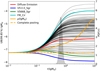 |
Fig. A.3. Same as Fig. 9 for 7Be. The x-axis has been extended to show the convergence to the no pooling estimate for large τ. |
Appendix B: Complete results table
Our complete results are presented in Table B.1.
Summary table of results for individual objects, diffuse emission, and pooling analysis.
All Tables
Summary table of results for individual objects, diffuse emission, and pooling analysis.
All Figures
|
Fig. 1. Distance distribution of CNe according to Eqs. (9) and (10) through rejection sampling. Shown are 104 samples (grey histogram, corresponding to a timescale of 200 yr, left axis), and an approximation with the Γ-distribution in red. The cumulative distributions are shown in black for the sample and in cyan for the Γ-distribution (right axis). |
| In the text | |
|
Fig. 2. Diffuse emission template from line-of-sight-integrated nova density distribution, Eq. (15), together with nova sample (cyan points). The contours indicate the De Vaucouleurs profile for the bulge and the exponential disc. |
| In the text | |
|
Fig. 3. Population synthesis of nova events in a Milky Way-like galaxy. Left: year 116.3 of the modelled Poisson process, where a nearby CO nova at (l, b) = (+123° , + 8° ) outshines the remaining galaxy in 478 keV emission (top). At the same time, 1275 keV emission is not enhanced (bottom). The angular resolution is chosen according to the SPI 2.7° (FWHM). Right: time profiles (light curves) of the 478 keV and 1275 keV since the beginning of the synthesis for a duration of ∼150 yr. This timescale is enough to reach convergence and to show characteristic features. The vertical purple line indicates the time shown in the plots on the left. |
| In the text | |
|
Fig. 4. Estimated S/N given the SPI data set (Sect. 3) and the range of plausible 22Na ejecta masses for our sample of 97 novae. Top: the S/N of individual objects does not increase with |
| In the text | |
|
Fig. 5. Exposure map of the selected data set. The effective areas around 478 and 1275 keV are ∼80 and ∼55 cm^2, respectively. |
| In the text | |
|
Fig. 6. Complete graph of different model variants used in this study. When the source models are used individually, that is, regardless of a common underlying physical process, the most conservative estimates are found in a no pooling setting (Sect. 5.2.1). The opposite extreme assumes that all objects eject the same amount of matter, so that instead of ∼100 different masses, only one is fitted. This resembles complete pooling and defines tight constraints but is subject to bias if the true variance is large (Sect. 5.2.2). A compromise between no and complete pooling is achieved by invoking the hyper-parameters μ and τ that determine the mean and the spread of ejecta masses, if any (partial pooling, dash-dotted box, Sect. 5.2.3). |
| In the text | |
|
Fig. 7. Summary of the no pooling analysis. Shown are the upper bounds (99.85th perc.) on the ejecta mass of 22Na for each object with known (orange) and unknown (black) distance. The dependence on distance lets the bounds on mass appear along the lines of constant flux (dashed lines). Full posteriors are given for objects with the best flux bound (V5115 Sgr), the best mass bound (V5113 Sgr), and whenever the significance is higher than 2σ (V1535 Sco). Theoretical expectations (Starrfield et al. 2009) are indicated by the green bands for 1.25 and 1.35 M⊙ ONe novae. Other theoretical expectations are bound to values below ≈ 10−8 M⊙ (e.g., José & Hernanz 1998). See text for a discussion of individual objects. |
| In the text | |
|
Fig. 8. Posterior distributions for diffuse emission of the 1275 keV line. The flux (top right) is separated into its two determining components, the 22Na ejecta mass (top left) and the ONe nova rate (bottom right, treated as a nuisance parameter). Theoretical predictions are indicated in green from Starrfield et al. (2009). The joint posterior (68.3th, 95.4th, and 99.7th percentile) of ejecta mass and nova rate (bottom left) shows the expected anticorrelated behaviour according to Eq. (17). |
| In the text | |
|
Fig. 9. Summary of the hierarchical model. Shown are the upper bounds on the 22Na ejecta masses (left axis) for individual objects (black) as a function of the population width τ, together with the complete pooling estimate (τ → 0, dashed orange), and the population mean μ (solid orange). Individual objects of interest (best (blue) worst (aqua) bound, diffuse emission (red)) are indicated. As τ → ∞, each upper bound converges to its no pooling value (Table B.1). Given the SPI flux posteriors, a population width of |
| In the text | |
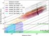 |
Fig. A.1. Same as Fig. 7 for the case of 7Be and the 478 keV line. |
| In the text | |
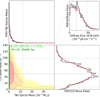 |
Fig. A.2. Same as Fig. 8 for the 478 keV line. |
| In the text | |
|
Fig. A.3. Same as Fig. 9 for 7Be. The x-axis has been extended to show the convergence to the no pooling estimate for large τ. |
| In the text | |
Current usage metrics show cumulative count of Article Views (full-text article views including HTML views, PDF and ePub downloads, according to the available data) and Abstracts Views on Vision4Press platform.
Data correspond to usage on the plateform after 2015. The current usage metrics is available 48-96 hours after online publication and is updated daily on week days.
Initial download of the metrics may take a while.