| Issue |
A&A
Volume 698, June 2025
|
|
|---|---|---|
| Article Number | A291 | |
| Number of page(s) | 10 | |
| Section | The Sun and the Heliosphere | |
| DOI | https://doi.org/10.1051/0004-6361/202453220 | |
| Published online | 23 June 2025 | |
Possible evidence for the 478 keV emission line from 7Be decay during the outburst phases of V1369 Cen
1
INAF, Osservatorio Astronomico di Capodimonte, salita Moiariello 16, I-80131, Naples, Italy
2
DARK, Niels Bohr Institute, University of Copenhagen, Jagtvej 155A, 2200 Copenhagen, Denmark
3
Julius-Maximilians-Universität Würzburg, Fakultät für Physik und Astronomie, Institut für Theoretische Physik und Astrophysik, Lehrstuhl für Astronomie, Emil-Fischer-Str. 31, D-97074 Würzburg, Germany
4
Institut de Recherche en Astrophysique et Planétologie, Université de Toulouse, CNRS, CNES, Université Toulouse III Paul Sabatier, 9 avenue Colonel Roche, BP 44346, 31028 Toulouse Cedex 4, France
5
INAF, Osservatorio Astronomico di Trieste, Via G.B.Tiepolo 11, Trieste, I-34143, Italy
6
Institute of Fundamental Physics of the Universe, IFPU, Via Beirut, 2, Trieste, I-34151, Italy
7
LIRA, Observatoire de Paris, Université PSL, Sorbonne Université, Université Paris Cité, CY Cergy Paris Université, CNRS, 92190 Meudon, France
8
Astrophysics Science Division, NASA Goddard Space Flight Center, Greenbelt, MD 20771, USA
⋆ Corresponding author: This email address is being protected from spambots. You need JavaScript enabled to view it.
Received:
29
November
2024
Accepted:
28
April
2025
Abstract
After decades of uncertainty about the origin of lithium, recent evidence suggests Galactic novae as its main astrophysical source. In this work, we present possible evidence for the first detection of the 7Be line at 478 keV, observed with the INTEGRAL satellite. The emission temporally and spatially coincides with the outburst of the bright nova V1369 Cen, where line significance ranges from 2.5σ to ∼1.9σ, depending on the detection methodology used. A bootstrap analysis, assuming a fixed full width half maximum of 8 keV, provides a flux of (4.9±2.0)×10−4 ph/cm2/s centred at 479.0 ± 2.5 keV, with a 2.5σ significant excess. This flux implies a total 7Be mass of M7Be = (1.2+2.0−0.6) × 10−8 M⊙ at the distance determined using several indicators, including the Gaia satellite. For a nova ejected mass estimated via radio observations, this result implies a 7Be=Li yield corresponding to A(Li) = 7.1+0.7−0.3. This value is comparable to those measured in a dozen novae through optical observations. Crucially, we confirm optically derived 7Li yields and demonstrate the groundbreaking potential of using gamma-ray data to measure Li abundances.
Key words: line: identification / nuclear reactions, nucleosynthesis, abundances / novae, cataclysmic variables
© The Authors 2025
 Open Access article, published by EDP Sciences, under the terms of the Creative Commons Attribution License (https://creativecommons.org/licenses/by/4.0), which permits unrestricted use, distribution, and reproduction in any medium, provided the original work is properly cited.
This article is published in open access under the Subscribe to Open model. This email address is being protected from spambots. You need JavaScript enabled to view it. to support open access publication.
1. Introduction
The origin of lithium (Li) is one of the most puzzling problems in modern astrophysics. It is the heaviest element formed in the Big Bang nucleosynthesis (BBN) and the only primordial species for which there is a tension between observations and theoretical predictions (Fields 2011). Moreover, the present Li abundance, as measured from meteorites or young T Tauri stars, is approximately four times higher than the BBN value and one order of magnitude higher than the abundance in old metal-poor stars (Spite & Spite 1982; Sbordone et al. 2010). Galactic lithium sources are required to explain its present abundance (Starrfield et al. 1978a; D’Antona & Matteucci 1991; Romano et al. 1999). After decades in which astrophysicists have been searching for answers about the origin of Li with no concrete clues about it, recently accumulated evidence suggests that Galactic novae might be the main Li factories of the Universe. One way to confirm that Li is produced in novae is by detecting the 478 keV emission line (Clayton 1981) corresponding to the decay of beryllium-7 (7Be) to Li through electron capture. Despite extensive searches, this long-sought-after emission line has still not been observed (Siegert et al. 2018).
Classical novae (CNe) are recurring thermonuclear explosions that occur in binary-star systems consisting of a white dwarf (WD) that is accreting matter from a main sequence star or an evolved companion (Bode & Evans 2008; Della Valle & Izzo 2020). When the pressure and temperature at the bottom of the accreted layer exceed the degeneracy pressure, thermonuclear reactions (TNR) ignite, removing degeneracy and causing the ejection of matter into the interstellar medium (ISM) (Starrfield et al. 1978b). The main fuel driving a CN explosion is the CNO reaction cycle, which leads to a rapid increase in the temperature and energy produced, and to the consequent ejection of a considerable amount of CNO isotopes into the ISM. During the TNR, the formation of beryllium-7 (7Be) occurs via the reaction 3He(α, γ)7Be, with 7Be being an unstable isotope that decays into 7Li via electron capture. The freshly-produced 7Be must be carried to the most external regions of the accreted layer by strong convective motions, which occur during the final stages leading up to the nova explosion. This process, known as the Cameron & Fowler (1978) mechanism, ensures that 7Be can survive the extreme conditions present in the hours or days immediately before the nova outburst.
7Be decays by electron capture through the reactions
 (1)
(1)
 (2)
(2)
 (3)
(3)
where 7Li* is a nuclearly excited state with an energy of 477.6 keV above the ground state. The laboratory value for the half-life time in reaction (2) is T1/2 = 53.12±0.06 days1 (Arnould & Norgard 1975), while for reaction (3) the branching ratio is 10.52%2. The detection of such a line associated with a nova outburst whose distance is known will provide a direct estimate of the Li yield (Hernanz et al. 1996).
Several attempts have been made in the last decades to detect the 478 keV line from novae, using a variegated suite of high-energy detectors (Harris et al. 1991; Siegert et al. 2021), which resulted only in upper limits on the flux of this line. More recently, Siegert et al. (2018) used the INTEGRAL/SPI detector to search for evidence of the γ-ray lines originating from radioactive decays, including the 478 keV line, in the bright nova V5668 Sgr. In this nova, a large amount of 7Be II was found in near-UV spectra obtained within the first 90 days from the nova explosion (Molaro et al. 2016). The lack of detection of the 478 keV line in INTEGRAL/SPI data is consistent with the distance of V5668 Sgr. One of the main outcomes from the work by Siegert et al. (2018) is that any emission from the 478 keV line from nova explosions should be sought in events at closer distances, namely d≤1 kpc.
2. The case of V1369 Cen
V1369 Cen is currently the brightest classical nova explosion observed in this century: it was discovered on December 3, 2013, and it immediately reached the de-reddened magnitude, V = 3.3 mag (Izzo et al. 2015). High-resolution optical spectra obtained seven days after its explosion pointed to the presence of an absorption feature that was attributed to the resonance line of neutral lithium Li I 670.7 nm, at the same expanding velocity of vexp=−550 km/s, similar to other line transitions identified for this nova (Izzo et al. 2015). Here we revisit the peak luminosity and the distance of V1369 Cen, based in particular on the acquisition of more accurate, multi-wavelength data, not available at the time of the nova explosion.
2.1. The maximum absolute magnitude of V1369 Cen
V1369 Cen has been extensively monitored by astronomers worldwide. The most detailed light curve of this nova was obtained using data collected by hundreds of amateur astronomers associated with the American Association of Variable Star Observers (AAVSO) (Kloppenborg 2023). The V-band light curve from their observations shows a multi-peaked structure, with a peak brightness of V = 3.3 mag (Izzo et al. 2015). This value is not corrected for the Galactic foreground extinction, AV. The literature provides an AV value of 0.5 mag (Mason et al. 2018), based on the relation between the equivalent width (EW) of the interstellar Na ID lines and the colour excess E(B−V) (Munari & Zwitter 1997). However, the Na ID IS lines in V1369 Cen spectra are saturated, indicating that the effective extinction is higher than this value (see also Appendix).
An alternative method involves using diffuse interstellar bands (DIBs) detected in the early bright phases of V1369 Cen's spectra. DIBs are known to correlate well with the neutral hydrogen in the ISM, and their intensities serve as good tracers of the total line-of-sight colour excess (Munari & Zwitter 1997; Raimond et al. 2012; Carvalho & Hillenbrand 2022; Schultheis et al. 2023), similar to other ISM lines. To determine the overall extinction to V1369 Cen, we first identified the presence of the DIBs at 578.0 nm, 661.4 nm, and 862.0 nm in the early bright spectra of the nova. We then measured the EWs of the absorption features generated by each DIB using the FEROS spectra of V1369 Cen on Day 7 and Day 14. Fortunately, the 862.1 nm DIB is located in a spectral region free from strong telluric lines. Figure 1 shows the identification and the region used for the EW measurement for each DIB, and Table 1 reports our measurements.
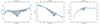 |
Fig. 1. DIBs identified in the early spectra of V1369 Cen and used for the estimate of the colour excess E(B−V). The grey area marks the region of the absorption line used for the EW measurement, respectively for the DIB 578.0 nm (left panel), the DIB 661.4 nm (middle panel), and the DIB 862.1 nm (right panel). |
DIB's EWs identified in the early spectra of V1369 Cen.
The colour excess E(B−V) is determined from DIB EWs using empirical correlations published in the literature and derived from high-resolution spectra of large samples of Galactic stars of all spectral types. The DIB at 578.0 nm is widely used in the literature due to its strong presence in stellar spectra. We refer to correlations found in large samples of early-type local (∼300 pc) stars with high-quality spectra (Raimond et al. 2012), in low-resolution (R∼3000) SDSS and LAMOST spectra of Galactic stars exhibiting a wide range of extinction (Yuan & Liu 2011), as well as in young stellar objects (Carvalho & Hillenbrand 2022). This latter sample was also used to correlate the DIB at 661.4 nm with colour excess, supported by a detailed study from the Gaia-ESO collaboration linking the EW of this DIB with total extinction along the line of sight in cool star spectra (Puspitarini et al. 2015). The DIB at 862.1 nm is one of the best tracers of the Galactic ISM spatial structure (Cox et al. 2024) and interstellar reddening. It shows a tight correlation with the colour excess along the line of sight of several stars (Raimond et al. 2012; Yuan & Liu 2011) and a clear correspondence with Galactic CO gas velocities (Carvalho & Hillenbrand 2022).
Using these extinction correlations and the DIB EW measurements from Table 1, we calculated a list of colour excesses. The weighted average of these values gives E(B−V) = 0.29±0.04 mag. Assuming a Cardelli et al. (1989) extinction curve, this results in a total V-band extinction of AV = 0.90±0.12 mag. Consequently, the de-reddened peak brightness of V1369 Cen is Vmax = 2.4±0.1 mag.
2.2. The distance to V1369 Cen
The distance to V1369 Cen is the most important parameter of the nova for which we do not have a precise estimate. Recent analyses suggest a range between d = 1.0±0.4 kpc, based on updated 3D Galactic reddening maps (Gordon et al. 2021), and up to 2.5 kpc, inferred from ISM lines and the H I 21 cm line profile (Mason et al. 2021). V1369 Cen was observed by the Gaia satellite (Prusti 2016) multiple times, with data release 3 (DR3) covering observations between July 25, 2014, and May 28, 2017 (Vallenari 2023). During this period, V1369 Cen was observed in 60 visits. The resulting parallax is p = 3.74±0.74 mas, and the distance inferred by a detailed Bayesian treatment of Gaia DR3 data is d = 643(+405,−112) pc (Schaefer 2022).
Interestingly, the distance derived using the General Stellar Parametrised from Photometry (GSP-Phot) methodology yields a much larger value. However, this method relies on Gaia Bp/Rp spectra matched to synthetic spectra from astrophysical models. The Gaia spectra of V1369 Cen, dominated by nebular spectral features from the 2013 outburst, do not resemble stellar templates, indicating that the GSP method is not applicable for V1369 Cen (Fig. 2). Additionally, given the extinction-corrected peak magnitude Vmax = 2.4 mag, the derived absolute magnitude at the GSP distance would be MV=−10.7 mag, which is much brighter than is typical for very fast novae (Della Valle & Izzo 2020). V1369 Cen, a moderately slow nova with t2 = 40±5 days (Izzo et al. 2015), suggests a fainter absolute magnitude.
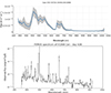 |
Fig. 2. Upper panel: Low-resolution Gaia spectrum of V1369 Cen obtained in 2015. Lower panel: High-resolution FEROS spectrum of V1369 Cen obtained on Feb. 3rd, 2015. The spectral features observed in the Gaia spectrum match the emission lines of the FEROS spectrum very well, indicating that the nova was in a similar spectral phase–the nebular stage–and that the spectrum does not have stellar features. This implies that the GSP methodology for deriving the distance of V1369 Cen cannot be applied to V1369 Cen. |
At the DR3 distance, the absolute magnitude at maximum would be Vmax=−6.6(+1.1,−0.3) mag, which is in agreement with expectations from the Maximum Magnitude and Rate of Decay (MMRD) relation (Della Valle & Izzo 2020). This relation links the absolute peak brightness of a nova with its decay rate, parametrised by the time a nova decays by two (to three) magnitudes, namely t2 (t3). Assuming the measured de-reddened peak brightness, Vpeak = 2.4±0.1 mag, and t2 = 40±5 days, we find that to conform to the MMRD relation within 2σ, V1369 Cen must be within 550 pc–1400 pc. Notably, the largest distance reported in the literature (Mason et al. 2021) is more than 3σ off the MMRD relation (see Fig. 3).
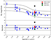 |
Fig. 3. Galactic MMRD relation estimated using the sample of novae whose distance was measured with Gaia (Della Valle & Izzo 2020). Dashed lines correspond to a 2σ confidence region. Red data marks the position of V1369 Cen using the distance derived from the use of the DIB 862.1 nm and Gaia stars in the surroundings of V1369 Cen. Black data marks the position of V1369 Cen at a distance of 2.4 kpc (Mason et al. 2021), while green data represents the position of V1369 Cen assuming a Gaia-DR3 distance (Schaefer 2022). |
We also use an alternative approach based on the correlation between the DIB at 862.1 nm and the colour excess for nearby stars. Distant stars exhibit more interstellar reddening, resulting in larger DIB EW values. We built a correlation between DIB EW and Gaia DR3 distance for stars near V1369 Cen. The Gaia collaboration has employed a similar method to study the Galactic ISM using the DIB at 862.1 nm in the RVS passband (Recio-Blanco et al. 2023). However, RVS spectra from Gaia DR3 are available only for stars brighter than 14 mag. From an initial sample of 625 stars, we identified 45 with Gaia-RVS spectra, of which only 21 were reliable for analysis due to a pipeline issue affecting 24 stars. The distribution of these stars, along with V1369 Cen at 970 pc, is shown in Fig. 4, with marker colour indicating DIB at 862.1 nm values.
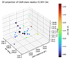 |
Fig. 4. Three-dimensional distribution of the sample of 21 Gaia DR3 stars surrounding V1369 Cen. The third spatial dimension is provided by the Gaia distance, while the colour of different markers corresponds to their respective DIB EW values. V1369 Cen is represented with a star, while the other Gaia DR3 stars are reported with circles. |
The distribution of DIB EW versus Gaia DR3 distance for these 21 stars is shown in Fig. 5. We performed a best-fit analysis that accounts for uncertainties in both the DIB EW and the Gaia distance, including an intrinsic scatter parameter. Using the ‘orthogonal’ method from the BCES python package (Nemmen et al. 2012), we found a correlation between DIB 862.1 nm EW and Gaia distance, shown as a black curve in Fig. 5, with 2σ uncertainty in dashed lines. Excluding three stars with DIB EW uncertainties larger than 0.1 mÅ did not significantly affect the result (shown as a red curve in the same figure). Consistent with Gordon et al. (2021) and the Gaia DR3 distance Vallenari (2023), the derived distance for V1369 Cen from the DIB measurement is dV1369Cen = 970.4±460.3 pc. Based on all the considerations reported above, we consider the distance to V1369 Cen the value reported in Schaefer (2022).
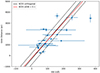 |
Fig. 5. Diffuse interstellar band 862.1 nm EW vs. Gaia distance distribution. The black curve represents the best fit identified from the entire sample of 21 stars, while the red curve refers to the same analysis performed on the stars characterised by an uncertainty on the EW < 100 mÅ. |
3. INTEGRAL observations of V1369 Cen
INTEGRAL has been observing the gamma-ray sky since its launch in 2002 (Winkler et al. 2003). During this time, more than a hundred Galactic novae have been detected in outbursts at optical wavelengths3. This number has been reduced by half since Gaia–a satellite dedicated to measuring parallaxes and proper motions of billions of stars in the Milky Way, including novae–became operational (Prusti 2016). We searched in the INTEGRAL archive for observations of the region in the sky where V1369 Cen was located, using a search radius value of ∼10 degrees.
INTEGRAL has observed in multiple visits the region of the sky surrounding the location of V1369 Cen. In particular, a dedicated target of opportunity observation was performed 24 days after the nova discovery, in order to follow up on the gamma-ray detection of the nova by the Large Area Telescope detector on board the Fermi spacecraft (Cheung et al. 2016). The list of INTEGRAL revolutions for which V1369 Cen is within the partially coded field of view of the Spectromètre Pour Integral (SPI), namely the angular distance to the pointing axis ≲16 deg, is reported in Table 2. This table in particular reports the time duration within the angular distance to the nova versus the detector direction to the sky, which is lower than 31 degrees. V1369 Cen never appeared in the fully coded field of view for revolutions with Rmin>8 deg. This implies that the effective area of the detector is reduced for those observations. In particular, during the revolution 1368 on December 27–24 days after the nova discovery–a dedicated ToO activation was carried out to observe gamma-ray transients (prog. ID 1040030, PI: den Hartog). During these observations, the angular distance of the direction to V1369 Cen and the pointing axis was indeed very small, varying slightly during the entire duration of the observations (texp = 90 ks) from 2.7 down to nearly zero degrees. Observations were executed using a hexagonal pattern.
Diary of INTEGRAL/SPI observations.
We performed a detailed analysis of INTEGRAL/SPI data for V1369 Cen for INTEGRAL revolution 1368. V1369 Cen was observed for approximately 90 ks in a hexagonal pattern with 15 among 19 active detectors. The gamma-ray spectrum was extracted from SPI/INTEGRAL data using a model-fitting method, which consists of fitting the flux of the source and the instrumental background rate in each energy bin to the counts measured per pointing and per detector. The instrumental background rate was fitted using two different methods (Siegert et al. 2019, but see also Section 1.3 of Siegert et al. 2018 and the method ORBIT-DETE in Section 3 of Knödlseder et al. 2005) yielding a difference in the flux of ≈11% (≈0.28σ). This systematic difference is smaller than the other statistical and systematic uncertainties (e.g. distance, date of the thermonuclear runaway) and is therefore not considered further (see also below). We began an analysis of the data from 20 keV to 505 keV and found that the spectrum is consistent with zero everywhere, except for a 2.5σ bump at exactly 478 keV, see Fig. 6. The reduced χ2 values in the range of the 478 keV line are displayed in Fig. 7. The flux in the remaining INTEGRAL/SPI range between 20 to 400 keV is consistent with zero flux, see also Fig. 8. The significance of this detection is strongly affected by the relatively short exposure time used during revolution 1368, which was the only observation where the nova's location was fully centred within the coded field of view of the SPI detector. To further assess systematics, we employed a third method that involved fitting a scaling factor to a fixed detector pattern (Isern et al. 2016) for each pointing and energy bin. This approach yielded a slightly lower significance with a difference of −0.59σ compared to the chosen value. In this method, the detector pattern was obtained using the relative background count rate between the detectors measured per orbit for each energy bin. Based on the above analyses, we conclude that the line significance varies from ∼1.9σ to 2.5σ, depending on the chosen background determination method.
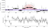 |
Fig. 6. Detection of the 478 keV line in INTEGRAL/SPI data during revolution 1368, obtained with analysis using a fixed Gaussian line width. Inspection of the full spectrum from 20 keV to 505 keV shows that it is consistent with zero everywhere except for the bump at 478 keV. The top panel shows the extracted fluxes (grey) and re-binned (black). The fitted spectrum is shown as a blue (constant) and red (line) band with their 1 and 2 sigma uncertainties. The bottom panel shows the residuals of the fit for the top panel (the plot for the line with a free line width is very similar). |
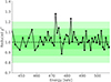 |
Fig. 7. Reduced χ2 values measured within the range surrounding the 478 keV line, for the fixed Gaussian model case. |
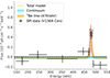 |
Fig. 8. Broadband spectrum of the position of V1369 Cen in INTEGRAL revolution 1368. Shown are extracted spectral data points from 150 keV to 550 keV, which are all consistent with zero except around the 478 keV line. |
Then we fit the spectrum in the restricted range between 445 and 505 keV, which includes the 478 keV line, using a constant model and an additional Gaussian line. We employed two different analyses. In the first analysis, we fixed the FWHM of the Gaussian line to the value of 8 keV FWHM, according to Siegert et al. (2018), obtaining an integrated photon flux for the line of FF=(4.9±2.0)×10−4 ph/cm2/s, with the line centre at 479.0+/−2.5 keV.
In order to more accurately evaluate the significance of the flux excess, we generated 1000 bootstrap samples using data from the SPI detector and the background flux in a 12 keV-wide band centred at 478.0 keV. This bandwidth corresponds to the full width at half maximum (FWHM) of approximately 8 keV for a Gaussian line. By comparing the two resulting distributions, we confirmed a 2.5σ significance level for the observed flux excess, see Fig. 10.
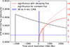 |
Fig. 9. Effective exposure time required to achieve a 5σ detection of the 478 keV line determined using the observed flux during revolution 1368 and the estimated explosion time of the nova. Assuming a constant flux over time for the 478 keV feature (red curve) and a decaying flux following the time decay of 7Be (red dashed curve), we find that an uninterrupted exposure time of 440 ks would be necessary. However, due to instrumental constraints (see text), this corresponds to an effective exposure time of approximately 780 ks to reach a 5σ detection. |
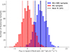 |
Fig. 10. Results of the bootstrap analysis described in the text. The red histogram represents 1000 resampled bootstrap datasets from the INTEGRAL/SPI containing background data, whereas the blue histogram illustrates samples from a band centred at 478.0 keV with a 12 keV width. Comparing these two distributions reveals an ≈2.5σ significance level for the observed sky flux exceeding the background, indicating a substantial detection of the spectral line. |
In the second analysis, we relaxed the constraint on the width of the line, obtaining an integrated photon flux of FT=(6.9±3.0)×10−4 ph/cm2/, and a width of FWHM = 3200 km/s. Figure 11 displays the normalised flux as a function of varying slit width. The results illustrate that a slit with a FWHM of approximately 8 keV yields the maximum flux. Consequently, the observation of the spectral line is exclusively detectable at this specific slit size.
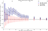 |
Fig. 11. Distribution of differential line fluxes normalised to the different extraction band widths at approximately 478.0 keV. Red data gives the result for the background region alone, while blue data corresponds to an extraction bin centred at 478.0 keV. The variation of the flux for different bin widths, with a maximum reached at about 8 keV, suggests that only for broad line widths, we obtain a significant signal for the line. |
Using Eq. (4), we can convert this estimate into the initial mass of 7Be synthesised in the outburst, after considering a delay time of t = 24 days from the nova discovery. Assuming a Gaia distance for V1369 Cen, we obtain a total 7Be mass of  M⊙, whereas in the case of a relaxed constraint on the FWHM of the Gaussian line, we measure a total synthesised mass of
  M⊙.
M⊙.
To determine the effective exposure time needed to achieve a 5σ significance detection for the 478 keV emission line, we performed simulations based on the flux measured during revolution 1368 and the expected explosion time of the nova. We considered two scenarios: (1) a constant line flux over time, and (2) a line flux that decays over time according to the mean lifetime  of the 7Be isotope. Our results indicate that an exposure time of t = 440 ks would have been required to achieve a 5σ significance detection for the 478 keV line (see Fig. 9). However, since the SPI detector can observe only approximately 85% of the 3-day INTEGRAL orbit, the effective exposure time needed to reach this significance level would be teff∼780 ks.
3.1. Swift Burst Alert Telescope observations and upper limits
We used the BatAnalysis python package (Parsotan et al. 2023) to analyse Swift Burst Alert Telescope (BAT) data from November 3, 2013, to December 10. We analysed survey data, where the location of V1369 Cen had at least a partial coding fraction of ∼19% on the BAT detector plane. The total set of observations that BAT took in the time period from 2013-11-03 to 2013-12-10 amounted to ∼2 581 303 s of exposure time, while the coordinates of V1369 Cen had a ∼19% partial coding or greater for 149 743 s of exposure time. Thus, BAT observed the target with a partial coding of ≳19% for ∼7% of the time.
We additionally constructed daily mosaicked images using the package to obtain potentially more significant detections of the nova. Overall, there was no significant detection of the nova in the BAT survey or daily mosaicked data. Using the BatAnalysis tool, we were also able to place upper limits on the nova emission in the 14–195 keV energy range for each survey and mosaicked dataset. We find that the flux upper limit in the 14–195 keV energy range is ≲6×10⁻⁹ erg/cm2/s 12 days before the nova was detected.
In Fig. 12, we show the count rate of the nova in panel (a), the measured signal to noise ratio (SNR) where it can be reliably determined in panel (b), the flux upper limits in panel (c), and the total exposure time of the source in panel (d). The grey points denote the survey-data-derived quantities, and the green points show the quantities obtained from the daily mosaics.
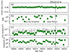 |
Fig. 12. Swift BAT observations of the location of V1369 Cen from 2013-11-03 to 2013-12-10. No significant detections of the nova were made, but upper limits can be placed on the 14–195 keV emission at the level of ≲6×10⁻⁹ erg/cm2/s, 12 days before the nova was detected. |
4. Discussions
The mass of 7Be synthesised in the TNR can be directly derived from the observed INTEGRAL/SPI photon flux F, using the following formula (Siegert et al. 2018):
 (4)
(4)
where  is the 7Be atomic mass and u is the atomic mass unit value. The quantity Δt represents the delay time between the ignition of the TNR and the moment at which the ejecta becomes optically thin to γ-ray photons (Siegert et al. 2018)–a value that is not well known, but likely to be of the order of a few days. We set this parameter to 5 days. Using Eq. (4), at the adopted distance of V1369 Cen, and considering t−Δt = 24 ± 5 days, we obtain a total 7Be mass of
  M⊙. In the case of the thawed FWHM, we measure a total synthesised mass of
  M⊙.
M⊙.
The ejected mass in V1369 Cen was obtained using data from the Australian Square Kilometer Array Pathfinder (ASKAP) during a systematic survey performed to search radio counterparts of CNe (Gulati et al. 2023). The ejected mass of V1369 Cen, at the distance of d = 1.0±0.4 kpc (Gordon et al. 2021), which is similar to the distance adopted in this work, is M=(1.65±0.17)×10−4 M⊙. However, this mass value was derived using a pure hydrogen composition for the nova ejecta in V1369 Cen. A more realistic assumption consists in considering a contribution from helium to the electron density population responsible for the observed radio emission. In the Hubble flow model for nova shells emitting at radio frequencies (Hjellming et al. 1979), a plasma with singly ionised helium and hydrogen, with a numerical abundance ratio of 0.15, was assumed. The contribution from heavier particles is negligible, given that the abundance of these elements in nova ejecta is of the order of 10−3–10−4 times lower than hydrogen (Gehrz et al. 1998). Considering this abundance ratio, and their density derived from ASKAP radio data, we determine the hydrogen and helium masses ejected in V1369 Cen to be Mej,H=(1.40±0.14)×10−4 M⊙ and Mej,He=(2.47±0.25)×10−5 M⊙. With these values and the 7Be mass found from an analysis of the 478 keV line, we obtain a total lithium yield of  , a value that is fully consistent with the average novae Li yield of logN(Li)/N(H)+12 = 7.34±0.47 derived from near-UV observations of a sample of Galactic and extra-Galactic novae in outburst (Molaro et al. 2023) (see Fig. 13). Moreover, a Li yield per nova event of A(Li) = 7.1 is approximately what is estimated to make the Li abundance observable (Cescutti & Molaro 2019). Lastly, the amount of Lithium measured from optical spectroscopy of V1369 Cen, MLi=(2.6±2.2)×10−10 M⊙ (Izzo et al. 2015), corresponds to only 8.7% of the total, considering the epoch of the spectrum (namely, t = 7 days) from the nova explosion, and the half-life decay time of 7Be, T1/2 = 53.12±0.06 days. Based on optical spectroscopy performed at the epoch of the nova outburst, the amount of the total 7Be synthesised during the TNR in V1369 Cen enriching the ISM is consequently
  M⊙ (see also Appendix). This is equivalent to a yield of N(Li)opt = 6.5±0.4, which is consistent with the value obtained from the analysis of the 478 keV line within 1σ (Fig. 13).
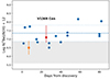 |
Fig. 13. 7Be yields measured in classical and recurrent novae from an analysis of the near-UV 7Be II 313.0 nm line (blue data). The plot shows the atomic ratio of 7Be to H: N(7Be) =logN(7Be)/N(HI)+12, on the y-axis. For V1369 Cen, the yield measured from the 478 keV line is N(7Be) = 7.1 |

5. Conclusions
In this work, we present possible evidence of the 7Be line at 478 keV, as predicted by Clayton (1981), and arising from the decay of beryllium-7 to lithium via electron capture. Despite extensive searches, this line has remained undetected until now (Siegert et al. 2018). The emission was observed by the INTEGRAL satellite during the explosion of V1369 Cen, the brightest nova observed so far this century.
The possible detected emission exhibits a flux of F=(4.9±2.0)×10−4 ph/cm2/s, which corresponds to a 2.5σ confidence level. Although indicative of potential gamma-ray activity at 478 keV, this significance level remains below the threshold required to assert an unequivocal detection. The flux excess is centred at 479.0 ± 2.5 keV and temporally and spatially coincides with the outburst of V1369 Cen. At a distance of d = 643(+405,−112) pc–determined using multiple methods, including observations from the Gaia satellite (Schaefer 2022)–this flux corresponds to a total 7Be mass of  M⊙. This value is higher than the average 7Be mass typically produced in nova events and is sufficient to account for the full amount of lithium estimated by Cescutti & Molaro (2019). By incorporating the total ejected mass of V1369 Cen, as determined from radio observations (Gulati et al. 2023), the atomic fraction of 7Be=Li in the outburst is calculated to be
  .
.
The analysis of the abundance obtained from the 478 keV line from 7Be decay aligns with previous 7Be and 7Li results obtained with near-UV and optical spectroscopy using ground-based telescopes in all novae where Li has been sought, see Fig. 13, thereby solidifying novae as main Li producers in the Milky Way. However, the derived Li abundances exceed theoretical predictions by a full order of magnitude, further highlighting the discrepancy with TNR calculations (Jose & Hernanz 1998; Rukeya et al. 2017; Starrfield et al. 2020).
Data availability
The INTEGRAL data used in this manuscript are publicly available on the INTEGRAL Cosmos website, hosted by the European Space Agency (ESA): https://www.cosmos.esa.int/web/integral/ integral-data-archives. The optical spectra of V1369 Cen are publicly available on the European Southern Observatory science archive facility: https://archive.eso.org/cms.html. The Python notebooks used in this analysis will be available in a dedicated repository hosted on GitHub publicly available personal page of the first author: https://github.com/lucagrb/V1369Cen
Acknowledgments
We want to thank the anonymous referee for their valuable comments and suggestions that greatly contributed to improving the quality of this manuscript. We also greatly appreciate Margarita Hernanz and Carme Jordi for the precious discussions and clarifications that have improved the structure of the manuscript. We also warmly thank Brad Schaefer for important discussions related to the Gaia distance to V1369 Cen and Jurgen Knodlseder for the support in the analysis of INTEGRAL/SPI data. The INTEGRAL/SPI project has been completed under the responsibility and leadership of CNES; we are grateful to ASI, CEA, CNES, DLR, ESA, INTA, NASA and OSTC for support of this ESA space science mission. PB acknowledges support from the ERC advanced grant N. 835087 – SPIAKID. LI acknowledges financial support from the YES Data Grant Program (PI: Izzo) Multi-wavelength and multi-messenger analysis of relativistic supernovae. We acknowledge with thanks the variable star observations from the AAVSO International Database contributed by observers worldwide and used in this research.
Corresponding to a mean lifetime of  days.
days.
References
- Arnould, M., & Norgard, H. 1975, A&A, 42, 55 [Google Scholar]
- Bode, M., & Evans, A. 2008, Classical Novae (Cambridge: Cambridge University Press) [CrossRef] [Google Scholar]
- Cameron, A. G. W., & Fowler, W. A. 1978, ApJ, 164, 111 [Google Scholar]
- Cardelli, J. A., Clayton, G. C., & Mathis, J. S. 1989, ApJ, 345, 245 [Google Scholar]
- Carvalho, A. S., & Hillenbrand, L. A. 2022, ApJ, 940, 156 [NASA ADS] [CrossRef] [Google Scholar]
- Cescutti, G., & Molaro, P. 2019, MNRAS, 482, 4372 [NASA ADS] [CrossRef] [Google Scholar]
- Cheung, C. C., Jean, P., Shore, S. N., et al. 2016, ApJ, 826, 142 [NASA ADS] [CrossRef] [Google Scholar]
- Clayton, D. D. 1981, ApJ, 244, 97 [Google Scholar]
- Cox, N. L. J., Vergely, J. L., & Lallement, R. 2024, A&A, 689, A38 [NASA ADS] [CrossRef] [EDP Sciences] [Google Scholar]
- D’Antona, F., & Matteucci, F. 1991, A&A, 248, 62 [NASA ADS] [Google Scholar]
- Della Valle, M., & Izzo, L. 2020, TAAR, 28, 1 [Google Scholar]
- Fields, B. D. 2011, Ann. Rev. Nuc. Part. Sci., 61, 47 [Google Scholar]
- Gaia Collaboration (Prusti, T., et al.) 2016, A&A, 595, A1 [NASA ADS] [CrossRef] [EDP Sciences] [Google Scholar]
- Gaia Collaboration (Vallenari, A., et al.) 2023, A&A, 674, A1 [NASA ADS] [CrossRef] [EDP Sciences] [Google Scholar]
- Gehrz, R. D., Truran, J. W., Williams, R. E., et al. 1998, PASP, 110, 743 [Google Scholar]
- Gordon, A. C., Aydi, E., & Page, K. L. 2021, ApJ, 910, 134 [NASA ADS] [CrossRef] [Google Scholar]
- Gulati, A., Murphy, T., Kaplan, D. L., et al. 2023, PASA, 40, 25 [Google Scholar]
- Harris, M. J., Leising, M. D., & Share, G. H. 1991, ApJ, 375, 216 [Google Scholar]
- Hernanz, M., Jose, J., Coc, A., et al. 1996, ApJ, 465, L27 [NASA ADS] [CrossRef] [Google Scholar]
- Hjellming, R. M., Wade, C., & Vandenberg, N. R. 1979, AJ, 84, 1619 [NASA ADS] [CrossRef] [Google Scholar]
- Isern, J., Jean, P., Bravo, E., et al. 2016, A&A, 588, A67 [NASA ADS] [CrossRef] [EDP Sciences] [Google Scholar]
- Izzo, L., Della Valle, M., Mason, E., et al. 2015, ApJ, 808, L14 [NASA ADS] [CrossRef] [Google Scholar]
- Jose, J., & Hernanz, M. 1998, ApJ, 494, 680 [Google Scholar]
- Jose, J., & Iliadis, C. 2011, Rep. Prog. Phys., 74, 9 [Google Scholar]
- Kloppenborg, B. K. 2023, Observations from the AAVSO International Database, https://www.aavso.org [Google Scholar]
- Knödlseder, J., Jean, P., Lonjou, V., et al. 2005, A&A, 441, 513 [NASA ADS] [CrossRef] [EDP Sciences] [Google Scholar]
- Lodders, K. 2021, Space Science Rev., 217, 44 [Google Scholar]
- Mason, E., Shore, S. N., De Gennaro Aquino, I., et al. 2018, ApJ, 853, 27 [Google Scholar]
- Mason, E., Shore, S. N., Drake, J., et al. 2021, A&A, 649, A28 [NASA ADS] [CrossRef] [EDP Sciences] [Google Scholar]
- Molaro, P., Izzo, L., Mason, E., et al. 2016, MNRAS, 463, 117 [Google Scholar]
- Molaro, P., Izzo, L., Selvelli, P., et al. 2023, MNRAS, 518, 2614 [Google Scholar]
- Munari, U., & Zwitter, T. 1997, A&A, 318, 269 [NASA ADS] [Google Scholar]
- Nemmen, R. S., Georganopoulos, M., Guiriec, S., et al. 2012, Science, 338, 6113 [Google Scholar]
- Parsotan, T., Laha, S., Palmer, D. M., et al. 2023, ApJ, 953, 155 [Google Scholar]
- Puspitarini, L., Lallement, R., Babusiaux, C., et al. 2015, A&A, 573, A35 [NASA ADS] [CrossRef] [EDP Sciences] [Google Scholar]
- Raimond, S., Lallement, R., Vergely, J. L., et al. 2012, A&A, 544, A136 [NASA ADS] [CrossRef] [EDP Sciences] [Google Scholar]
- Recio-Blanco, A., de Laverny, P., Palicio, P. A., et al. 2023, A&A, 674, A29 [NASA ADS] [CrossRef] [EDP Sciences] [Google Scholar]
- Romano, D., Matteucci, F., Molaro, P., et al. 1999, A&A, 352, 117 [Google Scholar]
- Rukeya, R., Lu, G., Wang, Z., et al. 2017, PASP, 129, 977 [Google Scholar]
- Sbordone, L., Bonifacio, P., Caffau, E., et al. 2010, A&A, 522, A236 [Google Scholar]
- Schaefer, B. E. 2022, MNRAS, 517, 6150 [NASA ADS] [CrossRef] [Google Scholar]
- Schultheis, M., Zhao, M., Zwitter, T., et al. 2023, A&A, 674, A40 [CrossRef] [EDP Sciences] [Google Scholar]
- Siegert, T. C., Coc, A., Delgado, L., et al. 2018, A&A, 615, A107 [NASA ADS] [CrossRef] [EDP Sciences] [Google Scholar]
- Siegert, T. C., Diehl, R., Weinberger, C., et al. 2019, A&A, 626, A73 [NASA ADS] [CrossRef] [EDP Sciences] [Google Scholar]
- Siegert, T. C., Ghogh, S., Mathur, K., et al. 2021, A&A, 650, A187 [NASA ADS] [CrossRef] [EDP Sciences] [Google Scholar]
- Spite, F., & Spite, M. 1982, A&A, 115, 357 [NASA ADS] [Google Scholar]
- Spitzer, L. 1998, Physical Processes in the Interstellar Medium (Wiley-VCH) [CrossRef] [Google Scholar]
- Starrfield, S., Truran, J. W., Sparks, W. M., et al. 1978a, ApJ, 222, 600 [NASA ADS] [CrossRef] [Google Scholar]
- Starrfield, S., Truran, J. W., & Sparks, W. M. 1978b, ApJ, 226, 186 [Google Scholar]
- Starrfield, S., Bose, M., Iliadis, C., et al. 2020, ApJ, 895, 70 [NASA ADS] [CrossRef] [Google Scholar]
- Steigman, G. 1996, ApJ, 457, 737 [CrossRef] [Google Scholar]
- Welty, D. E., Hobbs, L. M., & Morton, D. C. 2003, ApJS, 147, 61 [NASA ADS] [CrossRef] [Google Scholar]
- Winkler, C., Courvousier, T. J. -L., Di Cocco, G., et al. 2003, A&A, 411, 1 [Google Scholar]
- Yuan, H. B., & Liu, X. W. 2011, MNRAS, 425, 1763 [Google Scholar]
Appendix A: An accurate estimate of the lithium mass measured from the Li I 670.8 nm line
Here we revisit the measurement of lithium abundance in V1369 Cen (Izzo et al. 2015), using the curve of growth methodology, widely used to estimate physical properties, especially abundances, of an absorbing medium along the light of sight between the observer and the emitting source (Spitzer 1998), which in this case if the pseudo-photosphere from the underlying V1369 nova outburst. Thanks to the high resolution provided by FEROS, we have clearly identified and resolved the transitions from Li I, as well as from Na I and K I, namely elements that share with lithium the same electronic configuration in their most external orbitals (all of them are alkali metals), similar excitation energies for their ground state transitions and that they have been observed in their dominant ionisation state. However, the structure of V1369 Cen ejecta does not allow for a single fit for the entire absorption lines using a Gaussian or a Voigt model; this is particularly true for the Na ID doublet. In these cases, it is customary to use the equivalent width W of the entire absorption line, which is indeed a net measurement of the fraction of energy removed from the spectral continuum by the absorbing element in the ejecta, and then by the absorption line under consideration. From the equation of the radiative transport, and the assumption that the ejecta can be modelled as a thermal plasma with a given Maxwellian distribution described by a Doppler parameter b, we have that the specific equivalent width Wλ is proportional to (Spitzer 1998):
 (A.1)
(A.1)
where λ is the wavelength of the line transition under consideration, fij is the oscillator strength of the transition, Ni is the column density. The function F can be numerically integrated, providing a relation between the specific equivalent width and the column density for a given Doppler parameter b: the curve of growth.
Consequently, from an accurate measurement of the equivalent widths for the above-mentioned ground state transitions, it is possible to derive simultaneously the Doppler parameter b and the corresponding column densities. However, large column densities imply large optical depths, and then partial or complete saturation of the absorption line. When the absorption line is affected by saturation, the curve of growth starts to flatten, with the main consequence that a small variation in the equivalent width implies a large variation, and uncertainty, in the resulting column density, once b is determined.
We have used the Day 7 epoch spectrum to measure equivalent widths for ground state transitions of Na I D1 and D2 lines, the K I 769.9 nm, and Li I 670.8 nm lines. The K I lines are located in a region heavily affected by telluric lines. We have then performed a telluric correction by computing the telluric correction directly from the science spectrum, using a line-by-line radiative transfer model (LBLRTM4) with atmospheric input extracted from the science spectrum file header. This code attempts to best fit the observed spectrum by varying the composition of the atmosphere (water vapor and O2), as well as the pressure and the temperature to take into account possible variations within the total exposure time. However, despite this treatment, the K I 766.5 nm line profile cannot be fully recovered, given the presence of heavily saturated telluric lines at the same wavelengths of the P-Cygni absorption originating in the nova ejecta. Equivalent widths have been obtained by performing the following measurement for each absorption line:
 (A.2)
(A.2)
where i represents the single pixel wavelength (measured in Å), with Ic,i the continuum flux and Ii the observed flux at the pixel i.
To estimate the column density of lithium, we have developed a procedure that first performs a simultaneous best fit to search for the Doppler parameter b and the column density values of sodium, potassium, and lithium using their detected ground state transitions. The latter transition is a doublet, but separating the two lines is also difficult for a high-resolution spectrograph like FEROS, so we here have considered the Li I 670.8 nm feature as a single line. Then, we performed a Monte Carlo Markov Chain analysis, using the emcee ensemble sampler python package5, to estimate the posterior distributions, and then uncertainties, of the above parameters, obtaining the results displayed in Fig. A.1. The curve of growth corresponding to the best-fit b = 11.99 km/s, with the column densities derived for each single transition using this methodology, is shown in Fig. A.1. An immediate conclusion from this analysis is that sodium lines are saturated, located on the flat region of the curve of growth, and their best-fit column densities are not very precise. On the other hand, lithium  and potassium
  column densities are very well precise, being located in the linear region of the curve of growth, fig. A.1. Using only potassium as the reference element, we get an abundance ratio NLi/NK = 30/100, and after correcting for the differential ionisation of lithium of 0.54 (Steigman 1996; Welty et al. 2003) and adopting a solar abundance of N(KI) = 5.12±0.07 (Lodders 2021) we obtain an absolute N(Li) = 5.14±0.10.
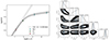 |
Fig. A.1. (Left panel) The best-fit curve of growth obtained from the equivalent width values measured in the Day 7 spectrum of V1369 Cen. Na I D lines are located in the flat region of the curve of growth, suggesting that they are saturated and hardly usable for precise abundance estimates (see also Fig. A.1). On the other hand, Ki and Li I lines are located in the linear region. This allowed us to estimate the lithium over-abundance and infer the amount of lithium mass in the nova ejecta from the Li I 670.8 nm absorption line. (Right panel) The posterior distribution for the Doppler parameter b and the column densities Ni derived from the MCMC procedure applied to the curve of growth best fit. |
Finally, we must consider that the total amount of 7Be that has already decayed into lithium on Day 7, namely when our abundance estimate has been performed, is provided by
 (A.3)
(A.3)
where T1/2 is the half-life time decay of 7Be, and uLi = 7. This value is 8.7% of the total initial abundance of beryllium, implying that the initial total abundance of lithium in the ejecta of V1369 Cen, as measured from the Li I 670.8 nm line, is N(Li) = 6.5±0.4. This value is in agreement with the respective uncertainties of the estimate obtained through the detection of the 7Be 478 keV line.
Appendix B: Gaia stars used for the estimate of V1369 distance using the DIB 862.1 nm
List of GAIA stars
All Tables
All Figures
|
Fig. 1. DIBs identified in the early spectra of V1369 Cen and used for the estimate of the colour excess E(B−V). The grey area marks the region of the absorption line used for the EW measurement, respectively for the DIB 578.0 nm (left panel), the DIB 661.4 nm (middle panel), and the DIB 862.1 nm (right panel). |
| In the text | |
|
Fig. 2. Upper panel: Low-resolution Gaia spectrum of V1369 Cen obtained in 2015. Lower panel: High-resolution FEROS spectrum of V1369 Cen obtained on Feb. 3rd, 2015. The spectral features observed in the Gaia spectrum match the emission lines of the FEROS spectrum very well, indicating that the nova was in a similar spectral phase–the nebular stage–and that the spectrum does not have stellar features. This implies that the GSP methodology for deriving the distance of V1369 Cen cannot be applied to V1369 Cen. |
| In the text | |
|
Fig. 3. Galactic MMRD relation estimated using the sample of novae whose distance was measured with Gaia (Della Valle & Izzo 2020). Dashed lines correspond to a 2σ confidence region. Red data marks the position of V1369 Cen using the distance derived from the use of the DIB 862.1 nm and Gaia stars in the surroundings of V1369 Cen. Black data marks the position of V1369 Cen at a distance of 2.4 kpc (Mason et al. 2021), while green data represents the position of V1369 Cen assuming a Gaia-DR3 distance (Schaefer 2022). |
| In the text | |
|
Fig. 4. Three-dimensional distribution of the sample of 21 Gaia DR3 stars surrounding V1369 Cen. The third spatial dimension is provided by the Gaia distance, while the colour of different markers corresponds to their respective DIB EW values. V1369 Cen is represented with a star, while the other Gaia DR3 stars are reported with circles. |
| In the text | |
|
Fig. 5. Diffuse interstellar band 862.1 nm EW vs. Gaia distance distribution. The black curve represents the best fit identified from the entire sample of 21 stars, while the red curve refers to the same analysis performed on the stars characterised by an uncertainty on the EW < 100 mÅ. |
| In the text | |
|
Fig. 6. Detection of the 478 keV line in INTEGRAL/SPI data during revolution 1368, obtained with analysis using a fixed Gaussian line width. Inspection of the full spectrum from 20 keV to 505 keV shows that it is consistent with zero everywhere except for the bump at 478 keV. The top panel shows the extracted fluxes (grey) and re-binned (black). The fitted spectrum is shown as a blue (constant) and red (line) band with their 1 and 2 sigma uncertainties. The bottom panel shows the residuals of the fit for the top panel (the plot for the line with a free line width is very similar). |
| In the text | |
|
Fig. 7. Reduced χ2 values measured within the range surrounding the 478 keV line, for the fixed Gaussian model case. |
| In the text | |
|
Fig. 8. Broadband spectrum of the position of V1369 Cen in INTEGRAL revolution 1368. Shown are extracted spectral data points from 150 keV to 550 keV, which are all consistent with zero except around the 478 keV line. |
| In the text | |
|
Fig. 9. Effective exposure time required to achieve a 5σ detection of the 478 keV line determined using the observed flux during revolution 1368 and the estimated explosion time of the nova. Assuming a constant flux over time for the 478 keV feature (red curve) and a decaying flux following the time decay of 7Be (red dashed curve), we find that an uninterrupted exposure time of 440 ks would be necessary. However, due to instrumental constraints (see text), this corresponds to an effective exposure time of approximately 780 ks to reach a 5σ detection. |
| In the text | |
|
Fig. 10. Results of the bootstrap analysis described in the text. The red histogram represents 1000 resampled bootstrap datasets from the INTEGRAL/SPI containing background data, whereas the blue histogram illustrates samples from a band centred at 478.0 keV with a 12 keV width. Comparing these two distributions reveals an ≈2.5σ significance level for the observed sky flux exceeding the background, indicating a substantial detection of the spectral line. |
| In the text | |
|
Fig. 11. Distribution of differential line fluxes normalised to the different extraction band widths at approximately 478.0 keV. Red data gives the result for the background region alone, while blue data corresponds to an extraction bin centred at 478.0 keV. The variation of the flux for different bin widths, with a maximum reached at about 8 keV, suggests that only for broad line widths, we obtain a significant signal for the line. |
| In the text | |
|
Fig. 12. Swift BAT observations of the location of V1369 Cen from 2013-11-03 to 2013-12-10. No significant detections of the nova were made, but upper limits can be placed on the 14–195 keV emission at the level of ≲6×10⁻⁹ erg/cm2/s, 12 days before the nova was detected. |
| In the text | |
|
Fig. 13. 7Be yields measured in classical and recurrent novae from an analysis of the near-UV 7Be II 313.0 nm line (blue data). The plot shows the atomic ratio of 7Be to H: N(7Be) =logN(7Be)/N(HI)+12, on the y-axis. For V1369 Cen, the yield measured from the 478 keV line is N(7Be) = 7.1 |
| In the text | |
|
Fig. A.1. (Left panel) The best-fit curve of growth obtained from the equivalent width values measured in the Day 7 spectrum of V1369 Cen. Na I D lines are located in the flat region of the curve of growth, suggesting that they are saturated and hardly usable for precise abundance estimates (see also Fig. A.1). On the other hand, Ki and Li I lines are located in the linear region. This allowed us to estimate the lithium over-abundance and infer the amount of lithium mass in the nova ejecta from the Li I 670.8 nm absorption line. (Right panel) The posterior distribution for the Doppler parameter b and the column densities Ni derived from the MCMC procedure applied to the curve of growth best fit. |
| In the text | |
Current usage metrics show cumulative count of Article Views (full-text article views including HTML views, PDF and ePub downloads, according to the available data) and Abstracts Views on Vision4Press platform.
Data correspond to usage on the plateform after 2015. The current usage metrics is available 48-96 hours after online publication and is updated daily on week days.
Initial download of the metrics may take a while.