© ESO 2021

1 Introduction

Oxygen is the third-most abundant element in the interstellar medium (ISM) after hydrogen and helium. Water is an important oxygen-bearing molecule in the formation of stars and planets.Water ice promotes the coagulation of dust grains from dense clouds to planet-forming disks (Chokshi et al. 1993; Testi et al. 2014; Schoonenberg & Ormel 2017), and water vapor is an important coolant of the gas in warm molecular environments (Neufeld et al. 1995), particularly in embedded protostellar systems (Karska et al. 2013). Ultimately, the delivery of water to young planets and small bodies conditions the emergence of life as we know it (Chyba & Hand 2005). Following the trail of water and its associated chemistry from clouds to young forming planets is a major goal of astrochemistry (van Dishoeck et al. 2014).

Infrared (IR) observations, supplemented by chemical modeling, have demonstrated that abundant ice is built at the surface of grains in cold dense clouds, locking in ~25% of the oxygen (Cuppen & Herbst 2007; Boogert et al. 2015). En route to the protostellar disk, condensed H₂O is released into the gas phase by passive heating from the accreting protostar (Ceccarelli et al. 1996)and jet-driven shocks (e.g., Flower & Pineau des Forêts 2012). Under these dense (n_H ≳ 10⁶ cm⁻³) and warm (T ≳ 200 K) conditions, oxygen chemistry is then driven by fast neutral-neutral reactions and photodissociation. In this context, the hydroxyl radical (OH) is a key reactive intermediate between atomic oxygen and water. The available gas-phase atomic oxygen is converted into OH by the reaction O + H₂ → OH + H, followed bythe formation of water through OH + H₂ → H₂O + H. OH is destroyed by the latter reaction, by the former reaction in the backward direction, and by UV photodissociation. Water is also destroyed either by the backward reaction H₂O + H → OH + H₂ or by photodissociation leading mostly to OH.

The observations of warm H₂O and OH vapor toward embedded protostars culminated with the Herschel Space Observatory (van Dishoeck et al. 2011), which outperformed previous far-IR and submillimeter observatories (e.g., SWAS, Odin, ISO-LWS). The detection of far-IR OH lines in inner envelopes and outflows (Wampfler et al. 2010, 2011, 2013; Goicoechea et al. 2015), supplemented by similar detections in prototypical photodissociation regions (Goicoechea et al. 2011; Parikka et al. 2017)and extragalactic sources (Sturm et al. 2011; González-Alfonso et al. 2012) evidenced the presence of an active warm oxygen chemistry in dense interstellar environments. One of the most striking results is the relatively low abundance of gaseous water found toward most of the protostellar sources, which contrasts with the abundant water ice supplied by the infalling envelope. In particular, multiple outflow components, which dominate H₂O emission, exhibit abundances ranging from 10⁻⁷ to 10⁻⁵ (Kristensen et al. 2012; Nisini et al. 2013; Kristensen et al. 2017). Water vapor from envelopes and perhaps embedded disks is typically traced by H${}_2^{17}$O and H${}_2^{18}$O lines and is best observed by Herschel-HIFI and (sub)millimeter interferometers (NOEMA, SMA, ALMA). While Visser et al. (2013) show that water abundance can be as high as 10⁻⁴, most of the protostellar systems exhibit lower water abundances, typically ranging between 10⁻⁷ and 10⁻⁵ (Jørgensen & van Dishoeck 2010; Persson et al. 2012, 2016; Harsono et al. 2020). Following the dissipation of the envelope, near- and mid-IR observations from space (e.g., Spitzer) and from the ground (e.g., VLT-CRIRES) have unveiled abundant hot water vapor in the planet-forming regions of Class II disks (≲ 10 au, Pontoppidan et al. 2014) but surprisingly dry Herbig disks (Pontoppidan et al. 2010; Fedele et al. 2011; Walsh et al. 2015).

The solution to this conundrum of low water abundance may lie in the impact of the ultraviolet (UV) radiation field produced by the accreting young star or strong jet shocks (V ≳ 40 km s⁻¹). Observations of hydrides provide evidence of the driving role of UV irradiation in the chemistry of protostars (Benz et al. 2016). It has been proposed that the low abundance of H₂O in protostellar outflows is the result of the UV photodissociation of H₂O vapor (Nisini et al. 2002, 2013; Karska et al. 2014). The low water abundance in embedded protostellar disks is generally attributed to the freeze-out of water (Visser et al. 2009). However, recent constraints on the thermal structures of Class 0 disk-like structures may contradict this interpretation (van ’t Hoff et al. 2020) and require the efficient destruction of H₂O or a large opacity of the dust in the far-IR.

The impact of UV photodissociation is generally explored by means of astrochemical models (van Kempen et al. 2010; Visser et al. 2012; Panoglou et al. 2012; Yvart et al. 2016). However, the strength of the local UV radiation field incident on disks, envelopes, and outflows is poorly known, due to the complex sources of UV emission and the unknown level of dust and gas attenuation on the line of sight, severely limiting the diagnostic capabilities. Assessing the exact role of UV photodissociation of water from astrochemical models based only on molecular abundances remains highly uncertain.

Alternatively, the excitation of molecular species provides in some cases a direct access to their formation and destruction routes. In irradiated regions, IR lines of H₂ and CO from ro-vibrationally excited levels trace the UV pumping followed by radiative decay (Krotkov et al. 1980; Black & van Dishoeck 1987) and have been used to probe the photodissociation of these species (Röllig et al. 2007; Thi et al. 2013). The excitation of reactive species for which the collisional time scale is comparable to the destruction time scale, carry also key information on their formation and destruction rates through a process called “chemical pumping” (Black 1998). So far, the incorporation of a state-to-state chemistry in models (i.e., models considering the state distribution of the reagents and the products) have been carried out only for a handful of molecular ions relevant for diffuse ISM and early Universe (Godard & Cernicharo 2013; Stäuber & Bruderer 2009; Coppola et al. 2013).

Mid-IR observations with Spitzer-IRS toward protostellar outflows and young disks evidenced the presence of a superthermal population of rotationally excited OH with energies up to E_up ≃ 28000 K (Tappe et al. 2008, 2012; Carr & Najita 2014). Two decades of extensive quantum calculations supplemented by laboratory experiments have permitted the direct interpretation of these observations as the smoking gun of H₂O photodissociation. Specifically, seminal works have shown that H₂O photodissociation through the à excited electronic state of H₂O (λ ≳ 143 nm) produces OH in vibrationally hot but rotationally cold states (e.g., Hwang et al. 1999a; Yang et al. 2000; van Harrevelt & van Hemert 2001), whereas photodissociation through the $\tilde{B}$ state (114 ≲ λ ≲ 143 nm) produces OH in high rotational states with levels up to N ≃ 47 (E ≃45000 K, Harich et al. 2000; van Harrevelt & van Hemert 2000). The rotationally excited lines of OH would thus probe the radiative cascade of OH products following their formation via H₂O photodissociation, a process called “prompt emission”. If consistently modeled, rotational lines of OH can thus give a direct access to the photodissociation of H₂O. However, a detailed modeling that includes chemical data accumulated over the past decades is lacking.

Probing H₂O photodissociation in astrophysical environments may also lead to unique constraints on the local UV irradiation field that H₂O is exposed to. The far-UV radiation field is a key parameter that controls the chemical, physical, and dynamical evolution of circumstellar regions. It regulates the overall chemistry of disk upper layers (e.g., van Dishoeck et al. 2006; Walsh et al. 2012) and outflows (Panoglou et al. 2012; Tabone et al. 2020), the thermal structure of disks (Gorti & Hollenbach 2004; Bruderer et al. 2012; Woitke et al. 2016), and the coupling between the gas and the magnetic field (e.g., Gammie 1996; Wang et al. 2019). The impact of the UV radiation field depends not only on attenuation processes, but also on its spectral shape. While the interstellar radiation field exhibits a broadband emission down to 91 nm (Habing 1968; Draine 1978; Mathis et al. 1983), the UV radiation emitted by accreting nascent stars (Bergin et al. 2003; Herczeg et al. 2004; Yang et al. 2012; Schindhelm et al. 2012) or by strong jet shocks (≳ 40 km s⁻¹, Raymond 1979; Dopita & Sutherland 2017) is often dominated by Lyman-α emission, leading to the selective photodissociation of species that exhibit large photodissociation cross sections at 121.6 nm.

To date, few robust diagnostics have been proposed to directly access the local UV radiation field. H₂ and CO lines excited by UV pumping probe only UV photons in narrow lines at < 114 nm that are rapidly attenuated and are not indicative of the broadband UV spectrum relevant for the other UV photoprocesses. Chemical diagnostics have also been proposed but they rely either on H₂ UV pumping (e.g., CN formed from excited H₂, Cazzoletti et al. 2018) or depend on elemental abundance ratios (e.g., hydrocarbons, Bergin et al. 2016).

In this work, we explore the potential of the OH mid-IR lines for probing H₂O photodissociation and the local UV radiation field under a broad range of physical conditions representative of dense irradiated environments, such as molecular shocks, circumstellar media, and prototypical photodissociation regions (PDRs). To reach this goal, results of quantum mechanical calculations resolving the electronic, vibrational, and rotational states of the OH product following H₂O dissociation at different UV wavelengths are collected. The distribution of the OH fragments following H₂O photodissociation by UV fields of various spectral shapes are derived. The emerging line intensities are then calculated using GROSBETA, anew molecular excitation code that includes prompt emission, radiative decay, collisional (de)excitation, and IR radiative pumping in a slab approach. For sake of conciseness, ro-vibrational lines of OH are not studied in this work.

In Sect. 2, we present the OH model and the basics of GROSBETA. The competition of the different excitation processes on the OH line intensities are studied in detail for H₂O photodissociation at Lyα (λ = 121.6 nm) and extended to other UV radiation fields in Sect. 3. In Sect. 4, a method to observationally derive the amount of H₂O photodissociated per unit time, the photodissociation rate of H₂O, and the strength of the local UV radiation field is proposed and applied to Spitzer-IRS observations of the tip of the HH 211 protostellar bow-shock. Our findings are summarized in Sect. 5.

2 Model

2.1 OH model

2.1.1 Energy levels

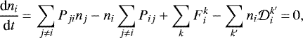
H₂O photodissociation can produce OH with high rotational and vibrational quantum numbers in the X²Π ground and the A² Σ⁺ first excited electronic states. Our OH model includes the energy levels provided by Brooke et al. (2016) and Yousefi et al. (2018) and made available on the EXOMOL database¹. Figure 1a shows the electronic, vibrational, and rotational levels included in the model. Regarding the ground electronic state OH(X²Π), vibrational levels up to v = 13 were included. We retained rotational levels that are stable against dissociation and in particular included energy levels above the dissociation energy of the OH(X) state that are stabilized by the centrifugal barrier (Chang et al. 2019). This corresponds to a quantum number of N = 54 in the v = 0 state, where N denotes the rotational quantum number associated with the motion of the nuclei. Each rotational level is further split into two spin–orbit manifolds corresponding to projected quantum numbers of the sum of the electronic orbital and spin angular momenta of Ω = 3∕2 and Ω = 1∕2 (see Fig. 1b). This results in two rotational ladders with fine-structure levels characterized by a total angular momentum quantum number of J = N + 1∕2 and J = N − 1∕2, respectively. Lastly, each rotational level (N, Ω) is further split by the Λ-doubling into two levels labeled by their spectroscopic parity index² e∕f. Our model includes the fine structure and Λ-splitting of the OH(X²Π)(v, N) states. Hyperfine structure is not considered in this work.

Regarding the OH(A²Σ⁺) state, levels with v ≥ 2 are dissociative (van Dishoeck & Dalgarno 1983) and the v = 0 with N ≥ 26 and the v = 1 with N ≥ 17 levels are predissociated (Yarkony 1992). Therefore, we limited the OH(A) levels to lower N of the v = 0, 1 states. The two rotational ladders emerging from the spin-orbit coupling of the OH(A²Σ⁺)(v) states were also taken into account. In the following, the electronic, vibrational, rotational, fine-structure, and parity states of OH are labeled as Λ, v, N, Ω, and ϵ, respectively.

2.1.2 Radiative transitions

Our OH model includes 54276 radiative transitions with their corresponding Einstein-A coefficients from Brooke et al. (2016) and Yousefi et al. (2018). The mid- and far-IR lines of OH originate from radiative transitions occurring within vibrational states (Δv = 0) of the OH(X) state (Fig. 1c). Figure 1b shows the radiative transitions that connect levels within a vibrational level of the X²Π ground state. The radiative transitions with the highest Einstein-A coefficients are the intra-ladder rotational transitions N → N − 1 (or equivalently J → J − 1) that preserve the e/f parity. These transitions give rise to lines from the mid- to the far-IR (see Fig. 1c). The cross-ladder transitions connecting the Ω = 1∕2 and Ω = 3∕2 states are of two kinds: J-conserving (ΔN = −1) and e∕f parity changing transitions, and J → J ± 1 (ΔN = 0, −2) and e∕f parity conserving transitions. Einstein-A coefficients of the latter two kinds are at least an order of magnitude lower than intra-ladder transitions and can be used to measure the opacity of the intra-ladder lines. Lastly, the Λ-doubling transitions, which lie from centimeter to sub-millimeter wavelengths, are also considered in this work. Rovibrational transitions follow the same selection rules and any rovibrational transition accompanied by any change of vibrational quantum number v′ → v″ is included in this work. Rovibrational lines v′ = 1 → v″ = 0 typically lie at near-IR wavelengths, around 2.7 μm. Transitions connecting to the OH(A²Σ⁺) state are electronic dipole allowed at near UV wavelengths.

2.2 Excitation by H₂O photodissociation

The OH state-specific formation rate associated with the photoprocess $${\text{H}}_2\text{O}+h\nu \to \text{OH}(\lambda ,\Lambda ,v,\text{N},\Omega ,ϵ)\text{+H}$$(1)

can be expressed as $$k(\Lambda ,v,N,\Omega ,ϵ)={\displaystyle {\int }_{\lambda }\eta }(\lambda ,\Lambda ,v,N,\Omega ,ϵ)\overline{\sigma }(\lambda )I(\lambda )\text{d}\lambda$$(2)

and measured in cgs units in s⁻¹. In this equation, η(λ, Λ, v, N, Ω, ϵ) is the probability of forming OH in a given state following H₂O photodissociation by a photon of wavelength λ, $\overline{\sigma }$ is the total photodissociation cross section (cm²) of H₂O → OH + H at that wavelength, and I(λ) is the photon flux averaged over all incidence angles (photon cm⁻² s⁻¹ cm⁻¹).

We assumed that the fine structure and Λ-doubling states of OH are equally populated by the photoprocess (1) so that η does not depend on Ω and ϵ. It is also convenient to define the nascent state distribution of the OH fragments as $$f(\Lambda ,v,N)=\frac{k(\Lambda ,v,N)}{\overline{k}},$$(3)

where $\overline{k}$ is the total rate for the photodissociation process (1). For a monochromatic UV radiation field emitting at a wavelength λ, f_i = η(λ, i).

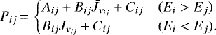
The absorption of a UV photon in the range 143–190 nm excites H₂O in its first excited singlet state à (first absorption band) and leads to a direct dissociation to OH + H. In this work, we adopted the OH state-specific cross sections computed by van Harrevelt & van Hemert (2001) using a wave packet approach. These data successfully reproduce the total photodissociation cross section of water in the considered energy range as well as the OH distributions measured by time-of-flight spectroscopy techniques (Yang et al. 2000). Figure 2a shows the distribution of the OH fragments following photodissociation by a photon of wavelength λ = 166 nm, where the cross section of the first absorption band peaks. Throughout the first absorption band, OH is produced in a rotationally cold (N ≲ 9) but vibrationally hot state (see also Appendix A). The proportion of vibrationally excited states increases with photon energy.

The absorption of a UV photon in the second absorption band ($\tilde{B}$ state of H₂O) results in a nonadiabatic transition, leading to OH in its ground electronic state and in a direct dissociation forming electronically excited OH. The second absorption band produces a broad continuum bump in the photodissociation cross section of H₂O in the range 114–143 nm. However, shortward of 124.6 nm, this dissociation channel coexists with the third and fourth absorption bands that result in sharper peaks in the photodissociation cross section (see Fig. A.3). As argued by van Harrevelt & van Hemert (2008), the $\tilde{C}$ and $\tilde{D}$ states are bound states and predissociated by the $\tilde{B}$ state. We consequently assumed that these channels lead to the same state distribution of the OH fragments as that via the $\tilde{B}$ state at the same photon energy. This is further supported by the agreement between experiments at λ ≤ 124 nm (e.g., Lyα, Harich et al. 2000)and theoretical work considering only the fragmentation dynamics from the $\tilde{B}$ state (van Harrevelt & van Hemert 2000, 2008). In the following, we use the term “photodissociation through the $\tilde{B}$ state” to refer to photodissociation in the range 114 to 143 nm. In order to obtain the relevant OH distributions, we repeated the quantum wave packet calculations as described in van Harrevelt & van Hemert (2000), but using the Dobbyn and Knowles potential (Dobbyn & Knowles 1997) instead of the Leiden potential since it was found that it gave better agreement with experiments (Fillion et al. 2001). In this wavelength range, H₂O photodissociation also leads to O with a branching ratio computed by van Harrevelt & van Hemert (2008). We used the total photodissociation cross section measured by Mota et al. (2005) that includes features due to the $\tilde{C}$ and $\tilde{D}$ states of H₂O (see Fig. A.3). The photodissociation cross section of H₂O → OH + H was then derived by taking into account the branching ratio of the OH forming channel as described by Heays et al. (2017).

As an example, we show in Fig. 2b the distribution of OH products at Lyα wavelength (λ = 121.6 nm). In contrast to photodissociation by lower energy photons, photodissociation in the range 114 to 143 nm produces OH(X²Π) with low vibrational excitation but high rotational excitation. OH is produced preferentially in the ground vibrational and electronic state, and the resulting rotational distribution within this state peaks around N = 45, corresponding to an energy level of ≃45 000 K. As shown in Fig. A.1, the peak in the rotational distribution increases with the photon energy from N ≃ 35 up to N ≃ 49. The other vibrational states follow a similar rotational distribution as that of the v = 0 state, but their relative contribution is much smaller, with less than 5% of OH produced in each of the OH(X)(v ≥ 1) states at Lyα. A fraction of OH is also produced in the excited electronic state OH(A) for λ < 137 nm. The rotational distributions of the v = 0, 1 states exhibit the same pattern as that of OH(X) but shifted toward lower N numbers.

Shortward of λ = 114 nm, photodissociation proceeds via even more excited electronic states of H₂O and systematic quantum calculations are lacking. Time-of-flight spectroscopy indicates that at λ = 115 nm OH distributions are vibrationally hotter than those computed through the $\tilde{B}$ but still rotationally hot (Chang et al. 2019). Photodissociation shortward of λ = 114 nm may also produce preferentially atomic oxygen instead of OH. In this work, we neglected the contribution of OH produced through photodissociation at wavelengths shorter than 114 nm.

Our adopted chemical dataset pertains only to water in the rotational ground state (“cold water”). Experimental data suggest that photodissociation of “warm water” could result in a small change in the rotational distribution of OH in the range N ≃ 32–40 (Hwang et al. 1999b). This change would however affect only lines coming from N ≳ 32 in the 9–10.5 μm range (see Sect. 3). Additionally, the adopted dataset does not include the fine-structure and the Λ-doubling states of the OH products. Recent theoretical investigations suggest that photodissociation through the $\tilde{B}$ state produces OH preferentially in the A′ symmetric states, which corresponds to the (Ω = 3∕2, e) and (Ω = 1∕2, f) states (Zhou et al. 2015). This asymmetry is also expected to depend on the rotational state of the parent H₂O, which is not considered here. New quantum calculations resolving the fine-structure and the Λ-doubling state and including the rotational state of the parent H₂O are needed to study in detail the A′∕A″ asymmetry. Our predictions presented in Sect. 3 remain valid by summing the line intensities over the fine-structure and Λ doublets of each N_up line.

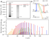Fig. 1 OH model adopted in this work. (a) X2Π and A2 Σ+ electronic levels split into vibrational levels and further split into rotational levels labeled by N (left ladder corresponding the OH(X2Π)(v = 0) state). The red line indicates the dissociation energy of OH(X2Π). (b) Structure of the rotational ladders of OH(X2Π) within a vibrational state that gives rise to mid- and far-IR lines. Each N level is split by the spin-orbit coupling and the Λ-doubling. The two spin-orbit states are labeled by the Ω quantum number and the Λ-doubling states are labeled by their ϵ = e∕f spectroscopic parity. Radiative transitions included in our model and emerging from the four N-levels are also depicted by arrows. There are three kinds of transitions: intra-ladder rotational transitions (blue and red arrows), cross-ladder transitions (green, with ΔN = − 1, and orange, with ΔN = 0, −2), and Λ-doubling transitions (purple). (c) Optically thin LTE spectrum of OH at TK = 750 K. The color code is the same as panel b) and is repeated in Figs. 4 and 9. The upper N level is indicated for some transitions. The Λ-doubling lines are too weak and at longer radio wavelengths to appear in this spectrum. Ro-vibrational lines are at shorter wavelengths than shown here (λ ≲ 2.7 μm).

Fig. 2 State distribution of the OH product following H2O photodissociation at two photon wavelengths. (a) At λ = 166 nm, H2O dissociating via its first excited à electronic state and producing OH in rotationally cold but vibrationally hot states. (b) At λ = 121.6 nm, H2O dissociating via its second excited $\tilde{B}$ electronic state and producing OH in rotationally hot but vibrationally cold states. Vibrational quantum numbers are color coded as indicated in the top panel. The distributions within OH(X2Π, v) and OH(A2Σ+, v) are plotted in solid and dashed lines, respectively, as a function of the rotational quantum number N. Only vibrational levels that contribute at least 1.5% to the population of nascent OH are shown.

2.3 OH excitation

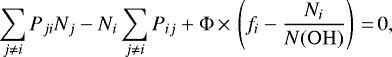
When radiative processes dominate, the emitted spectrum of OH will be governed by the state-specific dissociation rates of H₂O (see Eq. (2)) and by the spontaneous transition probabilities in the subsequent cascade of vibronic and rotational transitions. This is called the prompt spectrum of OH. In astrophysically relevant conditions, excited states of OH can be populated in steady-state by various other collisional and radiative processes, and these excited molecules also contribute to an observable spectrum. Thus the true population of excited OH differs from the nascent population.

In this work, the OH level populations and the line intensities were computed with a new code named GROSBETA (Black et al. in prep.). This code is based on a single-zone model, following the formalism presented in van der Tak et al. (2007) and implemented in the RADEX³ code. Under the assumption of statistical equilibrium, the local population densities, denoted n_i (cm⁻³), are given by $$\frac{\text{d}{n}_i}{\text{d}t}={\sum }_{j\ne i}{P}_{ji}{n}_j-n_i{\sum }_{j\ne i}{P}_{ij}+{\sum }_k{F}_i^k-{\sum }_{k^{\prime }}{n}_i{\mathcal{D}}_i^{k^{\prime }}=0,$$(4)

where $F_i^k$ and $n_i{\mathcal{D}}_i^{k^{\prime }}$ are the formation and destruction rates (cm⁻³ s⁻¹) for level i = (Λ, v, N, Ω, ϵ) and are associated with the chemicalreactions labeled k and k′, respectively. The P_ij are the radiative and collisional transition probabilities i → j given by $$P_{ij}=\{\begin{array}{ll}{A}_{ij}+B_{ij}{\overline{J}}_{{\nu }_{ij}}+C_{ij}\hfill & (E_i>E_j)\hfill \\ B_{ij}{\overline{J}}_{{\nu }_{ij}}+C_{ij}\hfill & (E_i<E_j).\hfill \end{array}$$(5)

Here, A_ij and B_ij are the Einstein coefficients of spontaneous and induced emission, C_ij are the collisional rates (s⁻¹), and ${\overline{J}}_{{\nu }_{ij}}$ is the mean specific intensity at the frequency of the radiative transition i → j averaged over the line profile. As in van der Tak et al. (2007), the contribution of the lines to the local radiation field was computed following the escape probability method for a uniform sphere setting the line width to ΔV = 2 km s⁻¹. When all other physical parameters (e.g., density and temperature) are fixed, the solution depends only on the value of the ratio N(OH)∕ΔV.

The collisional (de)excitation rates in Eq. (5) were computed considering collision with H₂ and He for the OH levels within the v = 0 state using the rate coefficients from Offer et al. (1994) and Kłos et al. (2007), respectively. The rate coefficients computed by Offer et al. (1994) that include levels up to N = 5 have been extrapolated to higher N numbers (see Appendix B).

The induced radiative rates in Eq. (5) depend upon mean intensities ${\overline{J}}_{\nu }$ at the frequencies of all OH transitions. Thus the excitation model requires a specified ambient radiation field. Pure rotational and vibration-rotation transitions involve infrared radiation, which we parametrized as a blackbody intensity (Planck function) at a temperature T_IR times a geometrical dilution factor W. For illustration, we took W = 1. This gives a simple parametrization of the IR radiation field and a reasonably good proxy for the local radiation field in the far-IR regime relevant for the IR radiative pumping of pure rotational lines of the OH(X²Π)(v = 0) state. The impact of a more complex and realistic IR radiation field on the line intensities is briefly discussed in Sect. 3.1.2. Electronic transitions A − X respond to the near-ultraviolet. In this work, we neglected the impact of the near-UV radiative pumping.

The impact of formation and destruction of OH on its level population is described by the last two terms in Eq. (4). When activation barriers can be overcome (T_K ≳ 200 K), OH is primarily produced by the reaction of O atoms with H₂ and is rapidly converted into H₂O by the reaction with H₂. In turn, OH can also be regenerated from H₂O by UV photodissociation or by the reaction with atomic hydrogen. Photodissociation of OH, which is generally slower than H₂O photodissociation (depending on the spectral shape of the UV radiation field, see Heays et al. 2017), can also limit the abundance of OH. The formation and destruction routes are described by the state specific rates $F_i^k$ and ${\mathcal{D}}_i^{k^{\prime }}$, respectively.Their relative importance depends on the exact physical conditions. A complete model coupling chemistry and excitation of OH is beyond the scope of the present paper and for the sake of generality and conciseness, we made a number of simplifying assumptions to focus on the impact of H₂O photodissociation on OH excitation in various environments with a limited number of free parameters. The possible impact of O + H₂ on the excitation of OH is discussed in Sect. 4.2.2. In this work, we assumed that chemical steady-state holds, so that $$F\equiv {\sum }_k{\sum }_i{F}_i^k={\sum }_i{n}_i{\mathcal{D}}_i,$$(6)

where F is the total formation rate of OH (cm⁻³ s⁻¹), and 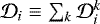${\mathcal{D}}_i\equiv {\sum }_k{\mathcal{D}}_i^k$ the total destruction rate of level i (s⁻¹). We also neglected any state selective destruction of OH assuming that OH is destroyed at the same rate for each state denoted here as $\mathcal{D}$ (i.e., ${\mathcal{D}}_i$ does not depend on i)⁴. Finally, we assumed that only H₂O photodissociation leading to OH modifies the level population of OH, with a state specific rate of F_i = n(H₂O)k(i), where n(H₂O) is the number density of H₂O and k(i) the state specific formation rate defined in Eq. (2).

Equation (4) can then be rewritten as an equation on the column density of OH in the levels i denoted as N_i, upon which line intensities depend. Assuming constant concentrations and excitation conditions along the line of sight, this yields $${\sum }_{j\ne i}{P}_{ji}{N}_j-N_i{\sum }_{j\ne i}{P}_{ij}+\Phi \times \left(f_i-\frac{N_i}{N(\text{OH})}\right)=0,$$(7)

with f_i the state distribution of the OH fragments as defined in Eq. (3) and $$\Phi \equiv N({\text{H}}_2\text{O}) \overline{k}$$(8)

the column density of H₂O photodissociated per unit time (cm⁻² s⁻¹). The state distribution f_i depends on the spectral shape of the UV radiation field. In this work, we explore UV radiation fields of various shape that are given in Fig. A.3, including narrow-band and broadband UV spectra.

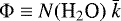
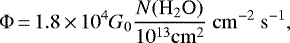
Equation (7) shows that Φ is the relevant parameter that ultimately controls the impact of prompt emission on the OH line intensities. The relation between the strength of the UV radiation field and Φ depends on its spectral shape. For a Lyα UV radiation field $$\Phi =1.8\times {10}^4{G}_0\frac{N({\text{H}}_{\text{2}}\text{O})}{{10}^{13}{\text{cm}}^{\text{2}}} {\text{cm}}^{\text{-2}} {\text{s}}^{\text{-1}},$$(9)

and for a Draine ISRF, 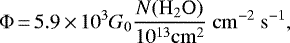$$\Phi =5.9\times {10}^3{G}_0\frac{N({\text{H}}_{\text{2}}\text{O})}{{10}^{13}{\text{cm}}^{\text{2}}} {\text{cm}}^{\text{-2}} {\text{s}}^{\text{-1}},$$(10)

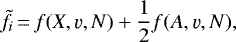
where G₀ is the intensity integrated between 91 and 200 nm, in units of the Draine (1978) radiation field (2.6 × 10⁻⁶ W m⁻², see also Heays et al. 2017). In this work we adopt Φ = 10⁷ cm⁻² s⁻¹ as a fiducial value and explore a broad range of values (see Table 1).

Φ can also be written as $$\Phi \equiv \mathcal{D}N(\text{OH}),$$(11)

where $\mathcal{D}$ (s⁻¹) is generally referred to as a destruction rate (see e.g., van der Tak et al. 2007; Stäuber & Bruderer 2009). Since chemical steady-state is assumed, $\mathcal{D}$ is also connected to the formation rate of OH. If other chemical reactions participate to the formation and destruction of OH (see Eq. (4)) and if these additional reactions form and destroy OH in proportion to their local population densities, then Eq. (7) still holds but $\mathcal{D}$ would not be associated with a destruction rate. $\mathcal{D}$ should rather be associated with a chemical pumping rate equal to the formation rate of the species by the considered process (in cm⁻³ s⁻¹) divided by its particle number density.

The line intensities were computed taking into account optical depth effects under the large velocity approximation. When calculating the line intensities, we assumed that the IR continuum background interacting with the gas is not along the same line of sight as the observations are taken. That is, the IR field contributes to the radiative pumping but not to the line formation. Throughout this work, we present line intensities I in erg s⁻¹ cm⁻², which are sometimes called emergent fluxes. That is, our I is related to the specific intensity in a line I_ν in erg s⁻¹ cm⁻² Hz⁻¹ sr⁻¹ by I = 4π∫ I_νdν. One can recover the observed line flux by the relation: $$F=\frac{I}{4\pi }\Delta \Omega ,$$(12)

where ΔΩ is the solid angle subtended by the source.

In otherwords, the populations and the line intensities of OH were computed from statistical equilibrium calculations involving prompt emission, IR radiative pumping and collisional excitation. Our model is controlled by six parameters summarized in Table 1: the spectral shape of the UV radiation field that determines the distribution of nascent OH denoted as f_i, the column density of H₂O photodissociated per unit time denoted as Φ, the column density of OH N(OH), the proton density n_H, the kinetic temperature T_K, and the temperature of the IR radiation field T_IR.

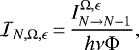
3 Results

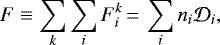
Figure 3 illustrates the difference between OH spectra following H₂O photodissociation through the à and $\tilde{B}$ state. Photodissociation via the H₂O à state leads to an OH spectrum dominated by far-IR lines coming from low rotational levels. H₂O photodissociation does not impact the mid- and far-IR spectrum since only collisions and IR pumping contribute to the excitation of those lines. In contrast, photodissociation through the H₂O $\tilde{B}$ state produces additional lines lying in the mid-IR coming from high-N states (15 ≲ N ≲ 45). These lines are produced by H₂O photodissociation. In this section, we shall identify the physical quantities that can be retrieved from the intensities of the mid- and far-IR lines. To do so, an in-depth study of the excitation mechanisms is provided in the case of photodissociation by Lyα photons (121.6 nm). The impact of a broadband UV radiation field, for which photodissociation proceeds through both the H₂O à and $\tilde{B}$ states is then studied.

3.1 Lyman alpha

As seen in Sect. 2.2, photodissociation of H₂O by Lyα photons produces OH in high rotational states (Fig. 2b). Figure 4 illustrates the influence of the column density of H₂O photodissociated per unit time denoted as Φ and of the column density of OH denoted as N(OH). The results of a more systematic exploration of the parameter space are presented in Fig. 5 by focusing on the intensities of three representative rotational lines that will be observed by JWST-MIRI (see Table 2).

3.1.1 High-N lines: prompt emission

The mid-IR spectrum (λ ≲ 20 μm) is dominated by pure intra-ladder rotational lines emerging from levels with high rotational quantum number (N ≥ 14), corresponding to upper energies >5000 K. Figure 4 shows that in this wavelength range, the line intensities are higher for a larger value of Φ (top and middle panels) but do not depend on N(OH) (top and bottompanels). The relative intensities of the intra-ladder lines depend neither on N(OH) nor on Φ so we focus on the intensity of the ²Π_1∕2(30, f) → ²Π_1∕2(29, f) line at 10.8 μm (see Table 2) as a proxy for the intensities of the mid-IR lines. Figure 5 (left panels) shows that the absolute line intensity is directly proportional to Φ and does not depend on other parameters such as N(OH), T_IR or n_H. This is one of the most fundamental properties of the high-N lines that makes them an unambiguous diagnostic of H₂O photodissociation.

This very simple result points toward a simple excitation process. Due to the high energy of the upper levels, IR radiative pumping does not contribute to the excitation of these lines. De-excitation by stimulated emission by the IR background is also negligible as long as the photon occupation number is much smaller than unity in the mid-IR domain, a condition that is fulfilled over the full parameter space. Due to the very high critical densities of these levels (n_crit ≳ 10¹³ cm⁻³), collisional (de)excitation is also negligible. Instead, the level populations, and the intensity of the lines coming from those levels, are set by the radiative cascade following the formation of OH in high-N states by H₂O photodissociation. The line intensities, or equivalently the number of radiative transitions per unit time between two excited levels, are then directly proportional to the formation rate of OH in higher excited states, which is proportional to the photodissociation rate of H₂O. The proportionality between the mid-IR line intensity and Φ is thus a direct consequence of the radiative cascade.

In order to analyze the relative intensity of the mid-IR lines, it is then convenient to define the normalized and dimensionless line intensity $${\mathcal{I}}_{N,\Omega ,ϵ}=\frac{I_{N\to N-1}^{\Omega ,ϵ}}{h\nu \Phi },$$(13)

where $I_{N\to N-1}^{\Omega ,ϵ}$ is the integrated intensity (in erg s⁻¹ cm⁻²) of the N → N − 1 line within the ladder Ω and the parity ϵ, and ν is the frequency of the line. As long as the population of the high-N levels is set by the radiative cascade, ${\mathcal{I}}_{N,\Omega ,ϵ}$ depends only on the distribution of nascent OH, or equivalently on the spectral shape of the UV field, and not on Φ or on any other physical parameter. Figure 6 shows that ${\mathcal{I}}_{N,\Omega ,ϵ}$ depends mostly on N and very little on Ω and ϵ. This is due to the fact that in our model, levels are assumed to be populated by H₂O photodissociation regardless of their Ω and ϵ states. In the following, we thus omit the reference to Ω and ϵ and note the normalized line intensity as ${\mathcal{I}}_N$. ${\mathcal{I}}_N$ increases with decreasing N, with a stiff rise between N = 47 and N = 35. This feature is also visible in Fig. 4 where the line intensities increase with wavelength between 9 and 10 μm. For 22 ≤ N ≤ 32, ${\mathcal{I}}_N$ is rather constant, corresponding also to a rather flat mid-IR spectra between 10 and 20 μm (see Fig. 4). This results in suprathermal excitation temperatures that vary between 2300 K for the lines at λ ≃ 20 μm up to 13000 K for the lines at λ ≃ 10 μm.

The normalized intensity ${\mathcal{I}}_N$ is directly related to the distribution of nascent OH. Interestingly, ${\mathcal{I}}_N$ can be interpreted as the probability that a photodissociation event H₂O → H + OH eventually leads to a radiative decay N → N − 1 via the radiative cascade. As such, ${\mathcal{I}}_N$ is necessarily smaller than unity. Because we assume the spin-orbit and Λ-doubling states to be equally populated by H₂O photodissociation, ${\mathcal{I}}_N\lesssim 1/4$. Owing to the selection rules, the rotational cascade within the v = 0 state is dominated by N → N − 1 transitions. Moreover, OH produced in an electronic level is shown to rapidly decay toward OH(X²Π) with little change of rotational number. Consequently, the formation of an OH fragment in an OH(Λ, v = 0, N′) state eventually leads to an intra-ladder transitions N → N − 1, with N ≤ N′. We plot in Fig. 6 (solid line) an analytical prediction of ${\mathcal{I}}_N$ assuming that transitions N → N − 1 are supplied by the radiative decay of the OH fragments produced in the v = 0 states (see model in Appendix C). This analytical expression relies only on the distribution of nascent OH denoted as f_i. The model reproduces the increase in ${\mathcal{I}}_N$ with deceasing N well, showing that its global variation with N is mostly due the fact that more and more OH fragments are added to the N → N − 1 rotational cascade as N decreases. The radiative cascade should then rather be seen as a “radiative river” that grows by its tributaries. In particular, the steep increase in ${\mathcal{I}}_N$ from N = 47 to 35 is due to the fact that most of the OH fragments are produced with these N-quantum numbers (see Fig. 2b).

We also note that for N < 35, our analytical model progressively underestimates ${\mathcal{I}}_N$. This is due to the contribution of the OH fragments produced in vibrationally excited states that are not included in our first analytical model. In Fig. 6 (dashed line) we show the analytical prediction of ${\mathcal{I}}_N$ assuming that any OH produced in an OH(Λ)(v, N) state immediately decays toward the OH(X²Π)(v = 0, N − 1) state. The model overestimates ${\mathcal{I}}_N$ showing that vibrationally excited states tend to undergo rotational transitions within v ≥ 1 vibrational states before decaying to the v = 0 state.

In other words, the spectral shape of the normalized intensity ${\mathcal{I}}_N$ is set by the population of nascent OH following photodissociation of H₂O. Our two simple analytical models, which rely only on the knowledge of the distribution of the OH fragments f_i, allow one to bracket ${\mathcal{I}}_N$.

Fig. 3 Infrared spectra of OH following H2O photodissociation at two photon wavelengths computed with GROSBETA. Top: at λ = 166 nm, H2O dissociating via its first excited à electronic state and producing rotationally cold OH. The OH infrared spectrum is dominated by far-IR lines excited by collisions and IR radiative pumping. Bottom: at λ = 121.6 nm, H2O dissociating via its second excited $\tilde{B}$ electronic state and producing rotationally hot OH. OH lines in the mid-IR with Nup = 20–45 trace H2O photodissociation through this electronic state. The density, temperature of the background radiation and kinetic temperature are fixed to their fiducial values (see Table 1) and Φ = 1010 cm−2 s−1. In this figure, all lines are colored red, even if coming from cross-ladder and intra-ladder transitions.

Fig. 4 Infrared spectra of OH depending on the column density of H2O photodissociated per unit time Φ and on N(OH) computed with GROSBETA for a Lyα UV radiation field. The density, temperature of the background radiation and kinetic temperature are fixed to their fiducial values (see Table 1). Following the color code used in Fig. 1, intra-ladder rotational lines are in red and blue and cross-ladder lines are in orange and green. Λ-doubling lines are too weak to appear here. The weak mid-IR lines lying in the range ~ 10–13 μm are intra-ladder rotational lines within the OH(X)(v = 1) state. The Nup rotational number of the upper energy level is indicated for selected lines.

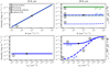Fig. 5 OH line intensities and the associated excitation processes as a function of Φ and nH for various values of N(OH) and TIR. The color indicates the value of N(OH) and the line style the value of TIR as defined in the right panels. The black circle indicates the fiducial model. The processes that dominate the excitation of the lines depending on the explored parameters are indicated along each curve. Left: intra-ladder rotational line at 10.8 μm coming from a high-N level (N = 30, Eup = 22600 K). This line depends only on Φ. Right: cross-ladder rotational line at 24.6 μm coming from a low-N level (N = 5, Eup = 875 K). This line traces the bulk population of OH. As such, it depends on N(OH), TIR and nH but does not depend on Φ.

Fig. 6 Normalized photon intensity of the OH(X2Π)(v = 0) intra-ladder mid-IR lines as a function of the quantum number of the upper energy level Nup. The photon intensities are computed for the fiducial values of the parameters and divided by Φ (see Eq. (13)). Circle and triangle markers correspond to lines belonging to the Ω = 1∕2 and Ω = 3∕2 ladders, respectively. Λ-doublets are indiscernible in this plot. In this regime, rotational levels are only populated by the radiative cascade of OH photofragments and ${\mathcal{I}}_{N,\Omega ,ϵ}$, depends only on the spectral shape of the adopted radiation field. The solid line is an analytical model that assumes that the intra-ladder lines within the v = 0 state are powered by the radiative cascade of the OH fragments produced in the v = 0 state. The dotted line is an analytical model that assumes that any OH produced in a vibrational state instantaneously decays toward the ground vibrational state with negligible change in its rotational number (see Appendix C).

3.1.2 Low-N lines

Figure 4 shows that, in contrast to the mid-IR lines, the far-IR lines (λ > 40 μm) do not depend on the column density of H₂O photodissociated per unit time Φ but on N(OH). The same conclusions apply to the cross-ladder transitions apparent from 20 μm to 114 μm. All these lines arise from N ≲ 6 levels (E_up ≲ 1200 K) and trace the bulk population of OH that is not excited by the radiative cascade from high-N levels. Because of the high optical depth of the intra-ladder lines, we focus in the following on the optically thin cross-ladder transition at 24.6 μm that arises from a N = 5 level (see Table 2). Figure 5 (right) shows for a broader range of parameters that the intensity of this line does not depend on Φ but on N(OH), T_IR, and n_H. Prompt emission is always negligible and the line intensity is the result of a competition between collisional (de-)excitation and IR radiative pumping.

Figure 5 (lower right panel) highlights three distinct excitation regimes as a function of density. At low density, the intensity does not depend on the density but on T_IR. In this regime, labeled by ②, levels are exclusively populated by IR radiative pumping. Because of our specific choice of the IR radiation field, all low-energy levels are thermalized to the same excitation temperature equal to T_IR and the intensities of the optically thin lines are $$I_{i\to j}\simeq A_{ij}{g}_i\frac{N(\text{OH})}{Q(T_{\text{IR}})}\frac{hc}{{\lambda }_{ij}}{e}^{-E_i/k_{\text{B}}{T}_{\text{IR}}},$$(14)

where Q(T_IR) is the partition function of OH. The intensity of the line at 24.6 μm is simply proportional to N(OH) and increases with T_IR. For an IR radiation field that deviates from a blackbody, the excitation of the OH(X²Π)(v = 0, N) levels is more complex. In this general case, the radiation brightness temperature T_rad varies with wavelength across the far-IR spectrum of OH (λ ≲ 120 μm). As a rule of thumb, the line intensity is then bracketed between our predictions with an undiluted blackbody at a value of T_IR that lies between the minimum and maximum values of T_rad.

At intermediate density, the intensity increases with n_H. For our fiducial values of T_IR and T_K, it corresponds to densities between 10⁸ and 10¹⁰ cm⁻³. In this regime, labeled by ③, collisions contribute to the excitation of the levels. However, line intensities also depend on T_IR, showing that IR radiative pumping is also relevant. Since the density is smaller than the critical density of the upper energy level (n_H ~ 10¹¹ cm⁻³), the de-excitation of the level is via radiative decay. Interestingly, the critical density above which collisions contribute to the excitation of the levels depends on T_IR and on T_K. It is lower for a lower T_IR (Fig. 5, bottom right) or for a higher T_K (not shown here). By comparing the rates of collisional excitation with the IR radiative pumping rate, collisions take over from IR radiative pumping in the excitation of a given N-level for $$n_{\text{H}}\gtrsim n_{\gamma }({\nu }_{\text{N}}) n_{\text{crit}} e^{h{\nu }_{\text{N}}/k_{\text{B}}{T}_{\text{K}}}\simeq n_{\text{crit}} e^{h{\nu }_{\text{N}}/k_{\text{B}}(1/T_{\text{K}}-1/T_{\text{IR}})},$$(15)

where ν_N denotes the frequency of the N → N − 1 radiative transition, n_γ is the photon occupation number, andwhere we assume hν_N ≫ T_IR for the second term. With n_crit having a weak dependence on T_K, the critical density above which collisions take over from IR radiative pumping depends on the contrast between the temperature of the gas and that of the radiation field.

Finally,above the critical density of the upper energy level (n_crit ≃ 10¹¹ cm⁻³), the line intensity converges toward its LTE value. In this regime, labeled by ④, collisions control the excitation and the de-excitation of the level and Eq. (14) gives the intensity of the optically thin line by substituting T_IR by T_K.

One hasto keep in mind that when IR radiative pumping is relevant for the excitation of a level, the geometry of the source turns out to be of great importance for the formation of the line coming from this level. We recall that the line intensities presented in this work are computed assuming that the IR background does not contribute to the line formation process. If the background IR field does contribute to the observed emission, lines can be weaker or seen in absorption (see OH lines observed by Wampfler et al. 2010, 2013). Collisions can also play a role in the formation of the line even when negligible in the excitation of the levels. Models incorporating specific source geometries are beyond the scope of this work and have already been explored to analyze low-N OH lines observed by Herschel toward protostars and photodissociation regions (Goicoechea et al. 2011; Wampfler et al. 2013).

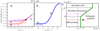Fig. 7 Transition from prompt emission to thermal or radiative excitation as revealed by the intensity of the intermediate N = 10 rotational line at 27.4 μm. The dominant excitation processes are indicated by ①, ②, ③, ④ as defined in Fig. 5. (a) Line intensity normalized by N(OH) as a function of $\mathcal{D}\equiv \Phi /N(\text{OH})$. The transition between prompt emission and radiative pumping or collisions depends on $\mathcal{D}$ and on nH. In particular, one can define a critical pumping rate ${\mathcal{D}}_{\text{crit}}$ below whichthermal or radiative excitation processes take over from prompt emission. (b) Line intensity normalized by N(OH) as a function of nH for $\mathcal{D}={10}^{-9} {\text{s}}^{-1}<{\mathcal{D}}_{\text{crit}}$. (c) Schematic parameter space indicating the dominant excitation process of the N = 10 line as a function of nH and $\mathcal{D}$. We note that whereas the specific values of $\mathcal{D}$ and nH reported in the x- and y-axis are for the N = 10 line, this schematic view remains valid for any rotational line. The prompt emission region is delimited by ${\mathcal{D}}_{\text{crit}}$ (green line). The regime ① corresponds to the excitation regime of high-N lines whereas the regimes ②, ③ and ④ correspond to the excitation regime of low-N lines. Panels (a) and (b) are cuts in the parameter space and are indicated by red, magenta and blue lines. The temperature of the IR background, the kinetic temperature and the column density of OH are fixed to their fiducial values. The other parameters are indicated in each panel.

3.1.3 Intermediate-N lines

We have shown in Sect. 3.1.1 that the high-N rotational lines excited by prompt emission are proportional to Φ and can thus be used to probe the photodissociation of H₂O. In contrast, low-N lines do not depend on Φ and trace the bulk population of OH. It is thus of a great importance to determine if a line coming from an intermediate-N level is indeed excited by prompt emission or by other processes such as IR radiative pumping or collisions.

Figures 7a and b shows that the intermediate − N line at 27.4 μm, which originates from a N = 10 level, shares features of low-N and high-N lines. This complex excitation pattern is the result of the competition between prompt emission, IR radiative pumping and collisions. Figure 7c summarizes the dominant excitation processes as a function of the density n_H and the chemical pumping rate $\mathcal{D}=\Phi /N(\text{OH})$ for the fiducial values of T_IR and N(OH).

For high values of the chemical pumping rate, the line intensity normalized by N(OH) is proportional to $\mathcal{D}$ (Fig. 7a). This corresponds to the right part of the parameter space shown in Fig. 7c. In this regime, the excitation of the upper energy level is dominated by prompt emission (regime ①) and we recover the result obtained for the high-N lines that the line intensity is proportional to $\Phi =\mathcal{D}N($OH) (Sect. 3.1.1). Figure 7a shows that below a critical value of the chemical pumping rate, denoted here as ${\mathcal{D}}_{\text{crit}}$, the intensity does not depend on $\mathcal{D}$ as IR radiative pumping or collisions take over from prompt emission. This corresponds to the left region of the parameter space (Fig. 7c). The excitation of the line as a function of the density then follows a pattern similar to that found for low − N lines (Fig. 7b). At low density, the excitation is dominated by IR radiative pumping (regime ②) whereas at higher density collisions progressively take over (regime ③). We find that for the fiducial values of T_IR and T_K, collisions contribute to the excitation of the line above n_H  ≃ 10⁸ cm⁻³. However, we recall that the effect of collisions on levels with N ≳ 5 is highly uncertain due to the lack of quantum calculations of collisional rate coefficients for these levels. In other words, the parameter space is divided into two regions: a region dominated by prompt emission for which results found in Sect. 3.1.1 apply, and a region dominated by other excitation processes for which results found in Sect. 3.1.2 apply.

The boundary between the two regions is defined by ${\mathcal{D}}_{\text{crit}}$ (green line Fig. 7c). Its value depends on the parameters that control the thermal and radiative excitation of OH, namely n_H, T_K, and T_IR. For example, Fig. 7a shows that ${\mathcal{D}}_{\text{crit}}$ increases from ~ 2 × 10⁻⁹ to ~ 2 × 10⁻⁸ s⁻¹ by increasing the density from n_H = 10⁷ to 10⁹ cm⁻³. Since ${\mathcal{D}}_{\text{crit}}$ quantifies the competition between thermal or radiative excitation and prompt emission, it also depends on the upper energy level of the line. We derive in Appendix E simple estimates of ${\mathcal{D}}_{\text{crit}}$ as a function of the excitation conditions (n_H, T_IR, and T_K) for any rotational level. In particular, we show that the schematic view of the parameter space proposed in Fig. 7c remains valid for the low-N lines for which the boundary is shifted to the right, and for high-N lines, for which the boundary is shifted to the left by orders of magnitudes.

3.1.4 Summary

The integrated intensities of the lines coming from high-N levels (N ≳ 20) are proportional to the column density of H₂O photodissociated per unit time and do not depend on other physical parameters. The shape of the mid-IR spectrum is only set by the distribution of the nascent OH and we define a normalized intensity of the intra-ladder lines, denoted as ${\mathcal{I}}_N$ (Fig. 6). The cross-ladder and intra-ladder rotational lines coming from low-N levels (N ≲ 6) are populated by IR radiative pumping or collisions and are thus tracing the bulk population of OH. Intermediate-N lines can be either excited by prompt emission, IR radiative pumping and/or collisions (see Fig. 7c).

3.2 Other UV radiation fields

3.2.1 State distribution of the OH fragments

Figure 8 shows the state distribution of the OH fragments following H₂O photodissociation by UV radiation fields of various spectral shapes. As shown in Sect. 3.1.1, the OH(A)(v, N) states decay toward the ground electronic state with little change of N. We consequently plot only the sum of the rotational distribution of OH(X) and OH(A) as defined by $${\tilde{f}}_i=f(X,v,N)+\frac{1}{2}f(A,v,N),$$(16)

where the factor $\frac{1}{2}$ stands for the different degeneracies between OH(A)(v, N) and OH(X)(v, N) states. The distribution of nascent OH computed from Eqs. (2) and (3) results from photodissociation at various wavelengths. As shown in Sect. 2.2, the distribution of the OH fragment η(λ, i) depends markedly onthe UV wavelength (see Fig. A.1). One of the most prominent differences is between photodissociation longward of λ = 143 nm, which produces OH(X) in low-N states, and photodissociation shortward ofthis value that produces OH(X) in high-N states and a small fraction of electronically excited OH(A) with N ≤ 27. The distribution of OH following H₂O photodissociation by a broad UV radiation field reflects the relative contribution of the different photodissociation channels. The fraction of photodissociation that proceeds through the two channels is given in Table 3.

We first study the effect a radiation field representative of the UV spectrum emitted by an accreting T Tauri star that includes a UV continuum plus emission lines (see Fig. A.3). As shown by Bergin et al. (2003) and Schindhelm et al. (2012), Lyα emission dominates over the continuum emission with ~90% of H₂O photodissociation done by Lyα photons. It results in a state distribution that is similar to that produced by a pure Lyα radiation field (Fig. 8a). Contribution of H₂O photodissociation through the H₂O Ã state (λ ≥ 143 nm), which represents ~ 10% of the total photodissociation rate, is however seen at N ≤ 6.

In contrast, a standard UV interstellar radiation field (ISRF) has a smooth and rather flat spectral distribution (Fig. A.3). H₂O photodissociation then proceeds through a broad wavelength range and results in a distribution of OH fragments that exhibits features of both photodissociation through the H₂O Ã and $\tilde{B}$ state (Fig. 8b). Photodissociation through the $\tilde{B}$ state creates a peak in the rotational distribution around N = 41 similar to that produced by photodissociation by Lyα, though somewhat smoother. OH(A) states are produced with a broad range of rotational quantum numbers, which results in a small bump in the rotational distribution that is perceptible in the range N = 10–27. We note that a significant fraction of the OH(A) products are dissociative and therefore not visible in Fig. 8b. Photodissociation through the H₂O Ã state, which represents 46% of the total photodissociation rate, yields to a prominent peak at low-N numbers.

A UV radiation field with a blackbody shape at T = 10 000 K has the steepest UV slope. Most of H₂O photodissociation proceeds through the à state. The resulting distribution of nascent OH is then dominated by low-N numbers whereas the bump at N ≃ 40 is reduced accordingly (Fig. 8c).

In other words, the state distribution of OH following H₂O photodissociation by a broad UV spectrum exhibits a bump at high-N number and a peak at low-N number. The amount of OH produced with high-N numbers is globally proportional to the fraction of photodissociation occurring through the $\tilde{B}$ state (λ < 143 nm).

Fig. 8 Rotational distribution of the OH fragments following H2O photodissociation by UV radiation fields of different shapes. The impact of three radiation fields is explored: (a) a radiation field representative of an accreting T Tauri star dominated by a Lyα emission line, (b) an ISRF radiation field and (c) a blackbody radiation field at 10 000 K. Vibrational quantum number are color coded as indicated in the top panel. The distribution is summed over the two electronic states. Only vibrational levels that contribute to at least 1.5% to the population of nascent OH are shown.

3.2.2 Mid-IR lines

As shown in the case of H₂O photodissociation by a Lyα radiation field, mid-IRlines are proportional to Φ. The same conclusion applies for any UV radiation field and we show in Fig. 9 the mid-IR spectrum emitted by OH for the UV radiation fields explored in this work, for the same value of Φ.

The mid-IR line intensities depend markedly on the shape of the radiation field. The main difference resides in the absolute line intensity between 10 and ~ 20 μm. For example, line intensities are ~ 5 times weaker for a blackbody at 10⁴ K than for a T Tauri radiation field. As seen in the case of a Lyα radiation field, mid-IR lines are fueled by the radiative decay of OH produced in high-N states. The absolute mid-IR line intensities are then proportional to the fraction of OH produced ina rotationally excited state, which is also proportional to the column density of H₂O photodissociated through $\tilde{B}$ state (cm⁻² s⁻¹) as defined by $${\Phi }^{\tilde{B}}\equiv N({\text{H}}_2\text{O}){\displaystyle {\int }_{114 nm}^{143 nm}\sigma }(\lambda )I(\lambda )\text{d}\lambda .$$(17)

This is further shown in Fig. 10, where the line intensities normalized by ${\Phi }^{\tilde{B}}$ as defined by⁵ $${\mathcal{I}}_{N,\Omega ,ϵ}^{\tilde{B}}\equiv \frac{I_{N\to N-1}^{\Omega ,ϵ}}{h\nu {\Phi }^{\tilde{B}}}$$(18)

are the about same for the different UV fields (within 20%). In other words, the absolute intensity of mid-IR lines traces the amount of H₂O photodissociated through the $\tilde{B}$ state (λ < 143 nm). It follows that the absolute intensity is, to a first approximation, only proportional to ${\Phi }^{\tilde{B}}$, regardless of the exact shape of the UV radiation field.

The other difference resides in the relative intensity of the lines, which reveals the precise shape of the rotational distribution of nascent OH fragments. This is best seen in Fig. 10. The increase in the line intensities from N_up = 46 down to N_up ≃ 35 is steeper for T Tauri and Lyα radiation fields than for the other two. These differences are due differences in the exact shape of the rotational distributions of the OH(X) fragments shown in Fig. 8. In the case of T Tauri and Lyα radiation fields, the peak at high-N is more pronounced than for the broadband UV spectra. The differences in the rotational distributions at lower N, which are mostly due to differences in the OH(A) distributions, result in minor differences in the line intensities in the range N_up = 25–15.

Fig. 9 OH mid-IR spectrum for various UV spectra computed with GROSBETA for Φ = 1010 cm−2 s−1. Other parameters are constant and equal to their fiducial values given in Table 1. Inthis regime, the intensity of intra-ladder lines (red and blue) are proportional to Φ and do not depend on other parameters such as TIR or nH.

Fig. 10 Normalized photon intensity of the OH(X2Π)(v = 0) intra-ladder mid-IR lines as a function of the quantum number of the upper energy level Nup. The intensities are computed for the fiducial values of the parameters (see Table 1) and normalized by the column density of water photodissociated via its $\tilde{B}$ state (see Eq. (18)). Circle and triangle markers correspond to lines belonging to the Ω = 1∕2 and Ω = 3∕2 ladders, respectively. Λ-doublets are indiscernible in this plot. In this regime, rotational levels are only populated by the radiative cascade of OH photofragments and ${\mathcal{I}}_{N,\Omega ,ϵ}^{\tilde{B}}$, depends only on the shape of the adopted radiation field.

3.2.3 Low and intermediate-N lines

Regarding far-IR lines and cross-ladder mid-IR lines, which emerge from N ≲ 6 levels, we find that the integrated intensities depend neither on the shape of the UV radiation field nor on Φ. This is a surprising result since UV radiation fields with a significant flux longward of 143 nm, produce OH with low rotational quantum numbers. Our finding indicates that the contribution of this rotationally cold population of nascent OH to the excitation oflow-N levels withinv = 0 is negligible compared to infrared pumping or collisions. The only population of nascent OH that affects the intensity of the rotational lines are the one produced with a high rotational number, typically N ≳ 15. However, we note that for much lower IR radiation fields and lower densities, these lines might be fueled by prompt emission (see Fig. 7c, regime ①). In that case, we expect to have a competition pattern between excitation via the H₂O Ã state and the $\tilde{B}$ state.

As studied in the case of photodissociation by a Lyα radiation field, intermediate-N lines can be excited either by prompt emission or IR radiative pumping and/or collisions. For a given set of physical parameters {T_IR, T_K, n_H}, the transition between prompt emission and the other excitation processes is controlled by the chemical pumping rate $\mathcal{D}\equiv \Phi /N(\text{OH})$ as summarized in Fig. 7c. The analysis proposed in Sect. 3.1.3 can be generalized to any UV radiation field by simply substituting $\mathcal{D}$ by ${\mathcal{D}}^{\tilde{B}}$ as defined by $${\mathcal{D}}^{\tilde{B}}={\Phi }^{\tilde{B}}/N(\text{OH}).$$(19)

We note that for the explored UV radiation fields, this adaptation has little impact on the transition between prompt emission and the other excitation processes.

4 Discussion and application to HH 211

In this section, we present a method for observationally inferring the photodissociation rate of H₂O and deducing the local UV radiation field. As an illustration, our model is applied to the Spitzer-IRS observations of the apex of the HH 211 bow-shock published by Tappe et al. (2008).

4.1 Diagnostics

4.1.1 Column density of H₂O photodissociated per second

Our results show that the absolute intensities of the intra-ladder lines in the mid-IR are proportional to the column density of H₂O photodissociated per second via the $\tilde{B}$ state, denoted as ${\Phi }^{\tilde{B}}$ (see Fig. 10). To our knowledge, the only alternative process that can also excite the rotational levels of energy E_up ≥ 20 000 K is the electron impact dissociation of H₂O (Beenakker et al. 1974; Bodewits et al. 2019). In some situations, such as disks around young stellar objects where there might be a source of energetic electrons (≳10 eV), the high-N OH lines would thus trace the destruction of H₂O via both e-impact and UV photodissociation. Complementary diagnostics, such as lines emerging from the triplet electronic states of H₂ or CO that can be excited efficiently by electron impact but not by UV absorption, can help to determine if OH lines might also trace the electron impact dissociation of H₂O. In this context, the predictions presented in this work remain valid as long as the destruction rate of H₂O by UV photodissociation dominates over destruction by e-impact, a condition that is generally satisfied in irradiated regions.

Consequently, the mid-IR lines of OH(X)(v = 0) provide a robust measurement of the column density of H₂O photodissociated in the range 114 to 143 nm. This key quantity can be observationally derived using the relation $${\Phi }^{\tilde{B}}=\frac{I_{N,\Omega ,ϵ}}{h\nu {\mathcal{I}}_{N,\Omega ,ϵ}^{\tilde{B}}},$$(20)

with ${\mathcal{I}}_{N,\Omega ,ϵ}^{\tilde{B}}$ provided in Fig. 10 and in Appendix D. As shown above, ${\mathcal{I}}_{N,\Omega ,ϵ}^{\tilde{B}}$ depends little on the spectral shape of the UV radiation field, and, in the absence of any other information, ${\Phi }^{\tilde{B}}$ can still be derived with a high accuracy (~10%). Interestingly, the time scale associated with the radiative cascade is about 10 ms, which is short compared with relevant dynamical time scales. Therefore, the value of ${\Phi }^{\tilde{B}}$ should be considered as an instantaneous measurement of the photodissociation activity. If the emitting region is unresolved, the derived value of ${\Phi }^{\tilde{B}}$ depends on the assumed source size as for any determination of a column density. Strictly speaking, the total flux integrated over a region on the sky gives the total number of H₂O molecules photodissociated per second in that region.

4.1.2 Spectral shape of the UV radiation field

The small deviations in the relative line intensities could be used to constrain the spectral shape of the radiation field (see Figs. 9 and 10). In particular, our results show that a Lyα dominated radiation field produces a steeper increase in the photon line intensities with decreasing N_up. However, detecting these small differences in the intensities in the range 9 to 11 μm requires an accurate relative flux calibration. In fact, the 10 μm silicate feature plays a significant role in the dereddening of the fluxes at visual extinctions A_V ≳ 10. In that perspective, the relative intensity of the lines between ≃9 and 10 μm in regions with high extinction should be interpreted with caution since the exact shape of the extinction curve varies significantly with A_v (Chapman et al. 2009; McClure 2009; Hensley & Draine 2020). We posit that a significant extinction in the mid-IR hampers the diagnostic capabilities of the OH lines to securely constrain the shape of the local UV radiation field. The impact of the rotational excitation of the parent H₂O may also complicate the interpretation of the relative line intensities and detailed quantum calculations are needed to propose robust diagnostics based on the exact shape of the OH mid-IR spectrum.

4.1.3 Photodissociation rate of H₂O

Our work shows that the detection of mid-IR lines of OH is prime evidence for the presence of H₂O, in particular in environments where the H₂O column density is limited by strong UV fields. If an independent measurement of the local UV radiation field can be observationally obtained, the column density of H₂O that it exposed to the UV field can be deduced as $$N({\text{H}}_2\text{O})=\frac{{\Phi }^{\tilde{B}}}{k_{\tilde{B}}},$$(21)

where $k_{\tilde{B}}$ is the photodissociation rate in s⁻¹ associated with H₂O → OH + H through the H₂O $\tilde{B}$ state.

Conversely, the OH emission can be used to measure the photodissociation rate $k_{\tilde{B}}$ by measuring the column density of water N(H₂O): $$k_{\tilde{B}}=\frac{{\Phi }^{\tilde{B}}}{N({\text{H}}_2\text{O})},$$(22)

where ${\Phi }^{\tilde{B}}$ is measured from the mid-IR lines of OH (see Eq. (20)). This quantity being a ratio between a column density and ${\Phi }^{\tilde{B}}$, it does not depend on the assumed source size.

The measurement of N(H₂O) is challenging and may be the major source of uncertainty in the determination of $k_{\tilde{B}}$. Besides the uncertainties that plague the determination of the column densities, the variation of the UV field and of the number density of H₂O along the line of sight may be an important bias. Indeed, irradiated environments exhibit a layered structure with physical conditions that vary steeply with distance, due to the attenuation of the radiation field or shocks. Because the OH mid-IR lines are optically thin and depend little on the shape of the UV radiation field, our predictions can be directly extended to any physical structure with $$I_N={\mathcal{I}}_N^{\tilde{B}}{\displaystyle {\int }_z{n}_{{\text{H}}_2\text{O}}}(z)k_{\tilde{B}}(z)\text{d}z,$$(23)

with $n_{{\text{H}}_2\text{O}}(z)$ the local number density of H₂O and $k_{\tilde{B}}(z)$ the local photodissociation rate of H₂O through the $\tilde{B}$ state. ${\Phi }^{\tilde{B}}$ being a quantity integrated along the line of sight, a spatial variation of the UV radiation field and of $n_{{\text{H}}_2\text{O}}(z)$ does not affect its measurement. On the contrary, $k_{\tilde{B}}$ is a local quantity and Eq. (22) should be applied with caution. Considerations on the geometry and on the viewing angle of the source may also help.

4.1.4 Local UV field

Our model shows that the OH mid-IR lines trace the photodissociation of H₂O by photons in the range 114–143 nm. As such, mid-IR OH lines carry information on the local UV radiation field in this range. In the following, we note $F_{UV}^{\tilde{B}}$, the photon flux integrated between 114 and 143 nm, which is $F_{UV}^{\tilde{B}}=6\times {10}^7$ cm⁻² s⁻¹ for a Draine radiation field. The photodissociation rate $k_{\tilde{B}}$ is the integral over the wavelength of the local UV radiation field multiplied by the photodissociation cross section: $$k_{\tilde{B}}={\displaystyle {\int }_{114 \text{nm}}^{143 \text{nm}}I}(\lambda )\sigma (\lambda )\text{d}\lambda .$$(24)

Strictly speaking, the conversion between $k_{\tilde{B}}$ and the local UV flux $F_{UV}^{\tilde{B}}$ should then rely on the knowledge of the shape of the UV radiation field. However, for the considered radiation fields, the intensity weighted cross section averaged between 114 and 143 nm varies only by a factor of ~3 and is about σ ≃ 6 × 10⁻¹⁸ cm². Thus, Eq. (24) can be approximated by $$F_{UV}^{\tilde{B}}\simeq \frac{k_{\tilde{B}}}{6\times {10}^{-18} {\text{cm}}^{\text{2}}},$$(25)

with a typical uncertainly of about a factor of three.

4.2 Application to HH 211

The Spitzer-IRS observations of the apex of the young protostellar jet HH 211 provide one of the best examples of highly rotationally excited OH. Figure 11 shows the unique sequence of superthermal OH emission lines unveiled from 10 μm down to 30 μm coming from rotational levels between N = 34 to N = 9. The association between OH mid-IR emission and ongoing H₂O photodissociation is further supported by the detection of a compact Hα emission by Walawender et al. (2006), tracing a strong UV emitting shock in the close vicinity of the OH emission. Complementary observations of H₂ rovibrational emission (2.12 μm, Hirano et al. 2006) and in the sub-millimeter domain unveiled a complex structure of multiple molecular bow-shocks encompassing the strong shock (Tappe et al. 2012).

4.2.1 Diagnostics from N > 20 lines

From the Spitzer-IRS spectrum published by Tappe et al. (2008), we measure a flux of the OH line at 14.6 μm of F = 3.5 × 10⁻¹⁵ erg s⁻¹ cm⁻² in an aperture of Ω = 1.9 × 10⁻⁹ sr. This line emerges from the N = 20 level of the OH(X)(v = 0) state and corresponds to an intensity integrated over solid angle of I = 2.3 × 10⁻⁵ erg s⁻¹ cm⁻² (see Eq. (12)). Figure 10 indicates that the conversion factor for each component of the quadruplet is ~ 0.2, regardless the spectral shape of the radiation field. At Spitzer-IRS spectral resolution (R ≃ 600 for the short-high module), the Λ-doublet and the fine-structure is however not spectrally resolved. Equation (20) then yields a column density of H₂O photodissociated per unit time of $${\Phi }^{\tilde{B}}=\frac{I}{4\times 0.2h\nu }=2.1\times {10}^8 {\text{cm}}^{\text{-2}} {\text{s}}^{\text{-1}},$$(26)

where the factor 4 stands for the sum over the four components of quadruplet, and ν is the frequency of the line. This corresponds to a total number of H₂O molecule photodissociated per second of 4 × 10⁴¹ molecules s⁻¹.

Figure 11 (top panel) compares a synthetic spectrum of OH produced by a Lyα radiation field with the Spitzer-IRS spectrum between 10 and 16 μm. We recall that in this wavelength range, the spectrum depends only on ${\Phi }^{\tilde{B}}$ and not on n_H, T_K or T_IR. Our model reproduces well the sequence of the lines coming from N = 31 down to N = 14.

The higher three lines lying in the range 10–10.5 μm are overestimated by the model. The extinction correction (A_v = 10 mag, Walawender et al. 2006)cannot explain this discrepancy since the extinction curve used by Tappe et al. (2008) tends to overestimate the extinction at 10 μm. An ISRF UV radiation field, which produces relatively weaker line fluxes shortward of 11 μm, does not significantly improve the fit. Alternatively, we posit that the rotational state of the parent H₂O could modify the rotational distribution above N ≃ 30. JWST observations with a higher signal-to-noise ratio, combined with modeling including the rotational state of the parent H₂O are required to clarify this.

${\Phi }^{\tilde{B}}$ can then be used to derive $k_{\tilde{B}}$, provided the column density of H₂O is known. Rotational lines of H₂O are detectedfrom the far-IR with Herschel-PACS to the mid-IR with Spitzer-IRS, spanning energy levels from 110 up to 1800 K. The mid-IR lines have been analyzed using GROSBETA and we derive a column density of ${2.2}_{-1.2}^{+2.0}\times {10}^{13}$ cm², a density of n_H ≃ 5 × 10⁷ cm⁻³, and a temperature of T_K ≃ 1300 K (see synthetic spectrum in Fig. 11, bottom panel). Interestingly, the same model reproduces the excitation temperature derived from the observations of far-IR lines (T_ex ≃ 90 K, Dionatos et al. 2018). This suggests that both mid-IR and far-IR lines trace the same warm H₂O reservoir that is photodissociated. Assuming a common origin for the OH and H₂O lines, Eq. (22) yields $$k_{\tilde{B}}\simeq 9.5\pm 4\times {10}^{-6} {\text{s}}^{\text{-1}}.$$(27)

The strong shock revealed by compact Hα emission is expected to produce a UV field dominated by Lyα photons. Equation (24) then gives 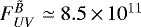$F_{UV}^{\tilde{B}}\simeq 8.5\times {10}^{11}$ photon cm⁻² s⁻¹, which corresponds to a UV photon flux 5 × 10³ times larger than that of the Draine ISRF in the range 91.2–200 nm. This value is well in line with models of fast dissociative shocks with V_S ≃ 50 km s⁻¹ and n_H ≃ 3 × 10⁵cm⁻³ (Raymond 1979; Lehmann et al. 2020), assuming that H₂O is produced in the warm postshock without further dilution of the UV radiation field. An origin of OH and H₂O emission in slower shocks passively illuminated by the stronger dissociative shock is also possible (see models of Melnick & Kaufman 2015; Godard et al. 2019). Spatially resolved observations with JWST-MIRI of both OH mid-IR lines and atomic lines that trace fast dissociative shocks such as [NeII] at 12.8 μm or [Ni II] at 6.6 μm (Hollenbach & McKee 1989) are required to distinguish the two possible scenarios.

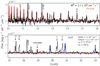Fig. 11 Comparison of the Spitzer-IRS mid-IR spectrum of the tip of HH 211 outflow from Tappe et al. (2008) (black lines) and of a synthetic GROSBETA spectrum for OH (in red) and H2O (in blue). The best fit parameters are indicated in the top right parts of the panels. The GROSBETA spectra are plotted assuming a source size equal to the extraction aperture ΔΩ = 1.9 × 10−9 sr. The rotational quantum number Nup are indicated for some OH lines. The model reproduces well the OH lines at 10–16 μm, but underproduces them at longer wavelengths.

4.2.2 Evidence of additional chemical pumping routes

Figure 11 (bottom panel) shows that the OH lines coming from lower N levels are detected with the Spitzer-IRS long-high module. In particular, the cross-ladder transition at 28.9 μm is well reproduced by our GROSBETA model with a column density of N(OH) = 2 × 10¹³cm⁻², assuming adensity of n_H = 5 × 10⁷cm⁻³ and a temperature of T_K = 1300 K derived from the H₂O lines. This model is illustrative since the emission of the OH cross-ladder line might originates from a different layer of gas but its suggests a N(OH)∕N(H₂O) ratio of about ≃0.9. This value lies in the upper part of the range 10⁻³ to 0.8 typically derived toward protostellar outflows, and is higher than those derived toward warm inner envelopes (Wampfler et al. 2011; Goicoechea et al. 2012, 2015). Interestingly, our derived ratio of ≃ 0.9 is closer to that estimated in low A_V regions of the Orion Bar (≳1, Goicoechea et al. 2011). This further supports the driving role of UV photodissociation in preventing the full conversion of OH into H₂O and in maintaining a relatively high N(OH)∕N(H₂O) ratio under warm conditions. Interestingly, detailed models of molecular shocks do predict that both, fast dissociative shocks and passively irradiated slow shocks exhibit high N(OH)∕N(H₂O) ratios (Neufeld & Dalgarno 1989; Godard et al. 2019; Lehmann et al. 2020).

For this set of GROSBETA parameters, the intra-ladder rotational lines longward of λ = 18 μm are underestimated by our GROSBETA model by up to a factor of eight. As shown in Sect. 3.1.3, these intermediate-N lines (9 < N < 15) are excited either by prompt emission, or by IR radiative pumping or collisions. In HH 211, the IR background detected by Spitzer-IRS is too weak to have a significant impact on the excitation of these levels. In fact, for the selected set of parameters, the excitation is dominated by prompt emission (right part of the schematic diagram, Fig. 7c). One could invoke collisional excitation to take over from prompt emission and increase the intensities of the intra-ladder transitions. This can be achieved by either decreasing the chemical pumping rate $\mathcal{D}$ or by increasing n_H and/or T_K (i.e., increasing ${\mathcal{D}}_{\text{crit}}$, see Fig. 7c). Because $\Phi =\mathcal{D}N($OH) is constrained by the lines in the range 10–16 μm, the intensity of the chemical pumping rate $\mathcal{D}$ can only be decreased by increasing N(OH). However, increasing N(OH), n_H or T_K would increase the intensities of the cross-ladder transitions, which are already well reproduced by our model. In other words, collisions or IR radiative pumping cannot reconcile our models with observations.

Interestingly, in this wavelength range, Λ doublets are spectrally resolved and show an asymmetry between A′ and A″ Λ-doublet states of about a factor of 1.5–2. As discussed by Carr & Najita (2014), this further supports the minimal impact of collisional (de)excitation since collisions might eliminate asymmetry in the population. This suggests that the intermediate-N transitions reveal another excitation process that is not included in our model.

The reaction H₂ + O can produceOH in rotationally and vibrationally excited states and supplement the excitation of intermediate-N levels. In particular, experimental data show that the reaction 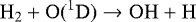$${\text{H}}_{\text{2}}\text{+O}{(}^{\text{1}}\text{D})\to \text{OH+H}$$(28)

produces OH with rotational number between N = 10 and 25 with a large fraction produced in v ≥ 1 and a propensity to the A′ states (Liu et al. 2000). Interestingly, the discrepancy between our predictions and the Spitzer-IRS spectra increases from N ~ 16 down to N ~ 9. The case of chemical excitation by reaction (28) can be treated in a similar way as we described the excitation of OH following H₂O photodissociation (see Sect. 3.1.1). In the case of H₂O photodissociation, the line intensities are given by the column density of OH formed by H₂O photodissociation. Similarly, reaction (28) will increase the line intensities in proportion to the number of OH produced per second via this reaction. The discrepancy between the model and the observations suggests that the formation rate of OH via reaction (28) is about 6 times larger than that via H₂O photodissociation. Interestingly, at the density derived by our non-LTE analysis of H₂O lines, O(¹ D) would be converted into OH instead of decaying via the radiative transition at λ = 6300 Å. However, this scenario requires an efficient production of O(¹ D), either by OH or H₂O photodissociation, or by collisional excitation. Still, the estimated column density ratio OH/H₂O appears to be too low for OH photodissociation to take over from H₂O photodissociation in the excitation of OH mid-IR lines. Moreover, at Lyα, only ~ 10% of the water photodissociation ends in O(¹D) (Slanger & Black 1982; van Harrevelt & van Hemert 2008), a fraction that is too small for the required efficiency of O(¹ D) production. Alternatively, the reaction between O(³P) and vibrationally excited H₂, known to be present at the tip of the bow-shock, could lead to OH in rotationally (and vibrationally) excited states (Gorti et al. 2011; Carr & Najita 2014). These additional chemical pumping routes could also impact the excitation of even lower-N lines. Further modeling combining OH excitation and chemistry is required to clarify the excitation of the intermediate-N lines.

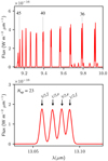Fig. 12 Expected OH mid-IR spectrum at JWST-MIRI resolving power (R ≃ 2000–3000). The parameters of the model correspond to those derived from the Spitzer-IRS observations of HH 211. The weak lines around 9.8 μm are pure rotational lines within the OH(X)(v = 1) state.

4.3 Perspectives with JWST-MIRI

JWST-MIRI will provide a unique view in the mid-IR regime by combining spectroscopic and imaging capabilities (Rieke et al. 2015; Wright et al. 2015). At the observed wavelength range (5–28 μm), JWST will be able to detect pure rotational lines coming from N ≥ 10 and cross-ladder lines coming from N ≥ 5, allowing for detailed studies of the excitation of OH across the full rotational ladder. In this section, we focus on the high-N rotational lines.

Up to now, OH mid-IR lines tracing H₂O photodissociation have been detected toward three protostellar outflows (Tappe et al. 2012) and a large number of protoplanetary disks (Pontoppidan et al. 2010; Salyk et al. 2011; Carr & Najita 2011, 2014). We predict that the jump in sensitivity will extend the detectabilityof high-N lines to other irradiated environments. Since the line intensities depend on the local abundance of H₂O and on the local radiation field, only astrochemical models designed for specific sources can robustly predict mid-IR line intensities. However, the detectability of the mid-IR lines as a function of the physical conditions can be explored with simple chemical arguments. The line emissivity per hydrogen atom depends on x(H₂O)G₀, where x(H₂O) is the H₂O abundance with respect to the total density of H atoms and G₀ the local UV flux (see Eq. (23)). In warm and irradiated environments (fast shocks, disk surface layers, low A_V depths of prototypical PDRs), one can assume that H₂O is destroyedby photodissociation and formed in the gas phase by two-body reactions so that x(H₂O) ∝ n_H∕G₀. For cooler regions, for which H₂O vapor is produced by photodesorption or by gas-phase ion-neutral routes, the scaling is expected to be different. Therefore, at least for warm environments, the emissivity of the OH lines per total hydrogen is expected to scale with the density. This may explain why superthermal OH emission has been detected by Spitzer in dense environments and remains undetected is classical photodissociation regions (Goicoechea et al. 2011). We thus posit that high-N lines could be detected by JWST-MIRI in more diffuse regions. Observation of dense prototypical PDRs such as the Orion bar or NGC 2023 should be considered as primary targets. In even more diffuse environments, such as translucent clouds, we expect OH mid-IR lines to remain undetected where we estimate Φ ≃ 10³−10⁴ cm⁻² s⁻¹ (Flagey et al. 2013), corresponding to line intensities as low as ~ 10⁻¹²−10⁻¹¹ erg s⁻¹ cm⁻² sr⁻¹.

The sensitivity of JWST will also allow us to probe the mid-IR emission in deeply embedded protostars. At high extinction (A_V ≳ 20), the OH lines in the range 13–15 μm will be particularly suited to minimize the IR extinction. The OH mid-IR emission can then constitute a unique tool to unravel the poorly known physical and chemical structure of young protostellar disks. Regarding protostellar jets and outflows, it will allow us to test if the low water abundance derived from Herschel observations is due to UV photodissociation or other physical processes (Karska et al. 2014).

The spatial resolution provided by mapping capabilities will also be crucial to constrain the emitting region of OH and map the photodissociation of H₂O. For dense environments, maps of N(H₂O) can be built from pure rotational lines of H₂O lying typically longward of 20 μm (E_up ≲ 1200 K) or ro-vibrational lines and used to construct maps of the local UV radiation field (see Eq. (25)).

The Medium Resolution Spectrometer (MIRI-MRS), with its relatively high spectral resolution (R ~ 2000–3000) will provide a valuable astrophysical view of H₂O photodissociation that will challenge current quantum calculations. Figure 12 shows a synthetic spectrum at MIRI-MRS spectral resolution. First, MIRI-MRS will give access to the OH lines in the range 9–10 μm that are directly populated by H₂O photodissociation (35 < N_up < 46, see also Fig. 8). The Λ-doublets and the fine-structure will be spectrally resolved up to N_up ≃ 29. This information will help to further constrain the shape of the UV radiation field and understand the impact of the rotational state of the parent H₂O. New quantum calculations, including the rotational state of H₂O, and the fine-structure and the Λ-doubling of the OH product, are warranted.

5 Conclusion

In this work, we explore the potential of the OH(X)(v = 0, N) mid-IR emission to probe H₂O photodissociation. To reach this goal, results from quantum mechanical calculations resolving the electronic, vibrational and rotational state of the OH product following H₂O photodissociation at different UV wavelengths are collected. The distribution of the OH photofragments is then calculated for UV fields of various spectral shapes and included in a new radiative transfer code called GROSBETA. The impact of prompt emission (i.e., formation of OH in excited states following H₂O photodissociation), collisional excitation and radiative pumping is extensively studied.

The main conclusions of this study are:

• 1.

  The mid-IR emission of OH in the range 9–16 μm is an unambiguous tracer of H₂O photodissociation. The mid-IR emission is the result of the rotational radiative cascade of OH photofragments within the v = 0 state. As such, the detection of these lines constitutes a prime evidence for the presence of active H₂O chemistry. In particular, the line intensities are directly proportional to the column density of H₂O photodissociated per second by photon in the range 114–143 nm, denoted as ${\Phi }^{\tilde{B}}$. The conversion factors between the line intensities and ${\Phi }^{\tilde{B}}$ is provided for each rotationally excited line and for UV radiation fields of various shapes in Fig. 10and in Appendix D. These conversion factors depend little on the exact spectral shape of the UV radiation field.

• 2.

  Provided a measurement of the column density of the irradiated water is known, the photodissociation rate by photons in the range 114–143 nm can be inferred (see Eq. (22)). The UV flux can then be deduced with good accuracy, regardless of the shape of the UV radiation field. Alternatively, provided an estimate of the strength of the local UV radiation field is available, the column density of H₂O can be derived.

• 3.

  The precise state distribution of the OH fragments depends on the spectral shape of the UV radiation field and results in small differences in the shape of mid-IR spectrum of OH. This suggests that the relative line intensities, if accurately measured, can be used to derive constraints on the spectral energy distribution of the UV radiation field.

• 4.

  The lower rotational levels, probed either by cross-ladder rotational lines shortward of 30 μm, or by far-IR rotational lines, are excited by IR radiative pumping or collisions. We provide criteria to determine if a rotational level of an intermediate energy (typically E_up = 3000 K, N ≃ 10) is excited by prompt emission or thermal processes.

• 5.

  As a test case, our model is applied to an irradiated region located at the tip of the HH 211 protostellar jet. Our simple single-zone model reproduces the Spitzer-IRS spectrum in the range 11–16 μm and shows that water is exposed to a UV photon flux that is about ~5 × 10³ times larger than the standard UV interstellar radiation field. Discrepancies between our predictions and the observations at longer wavelength suggest that additional chemical pumping processes such as the reaction H₂+O might contribute to the excitation of the rotational levels between N ~ 10–20.

• 6.

  JWST-MIRI will probe the rotational ladder of OH from N = 5 up to N ≃ 45 corresponding to energy levels from 800 K up to 45 000 K. We posit that the jump in sensitivity will unveil OH mid-IR emission in new environments such as prototypical photodissociation regions (e.g., Orion bar) and embedded protostars. Moreover, armed with good spectral resolution (R ~ 2000–3000), the MIRI-MRS observing mode will give access to even more excited lines in the range 9–10 μm and to the fine-structure and Λ-doubling state distribution of the OH fragments.

Our work demonstrates the potential of OH mid-IR lines to probe H₂O photodissocation and the strength of the UV field. New quantum calculations and astrochemical models taking into account the quantum state of the species are warranted to leverage future JWST observations and unveil oxygen chemistry through the excitation of OH.

Acknowledgements

The authors thank the anonymous referee for their constructive comments. B.T. would also like to thank B. Godard, A. Bosman and A. Faure for fruitful discussions. This work is part of the research programme Dutch Astrochemistry Network II with project number 614.001.751, which is (partly) financed by the Dutch Research Council (NWO).

Appendix A Distribution of OH fragments

In this appendix, we present the state distribution of OH following H₂O photodissociation as a function of the UV wavelength implemented in our model. The data stem from the quantum calculations published in van Harrevelt & van Hemert (2000, 2001). For the former, the calculations have been repeated using another potential energy surface that gives better agreement with experiments (see Sect. 2.2). As discussed in Sect. 2.2, we denote as η(λ, Λ, v, N) the probability to form OH in the state OH(Λ)(v, N) following H₂O photodissociation by a photon of wavelength λ. Figure A.1 shows the rotational distributions of OH as function of the photon wavelength for different electronic and vibrational states. Figure A.2 gives the vibrational distributions for each electronic state. The distributions shown in Figs. A.1 and A.2 do not account for the subsequent dissociation of the OH products. For example, the OH(A) rotational levels with v ≥ 2 are dissociative and are thus discarded in our excitation calculations.

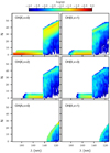Fig. A.1 Rotational distributions of nascent OH for various vibrational and electronic states as a function of the photodissociation wavelength. The OH distributions are summed over fine-structure and Λ-doubling states. The difference in the rotational distribution between photodissociation through the à (λ > 143 nm) and $\tilde{B}$ (λ < 143 nm) states of H2O is clearly visible.

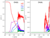Fig. A.2 Vibrational distributions of nascent OH for the two electronic states of OH as a function of the UV wavelength. The distributions η are summed over rotational, fine-structure and Λ-doubling states. The difference in the vibrational distribution between photodissociation through the à (λ > 143 nm) and $\tilde{B}$ (λ < 143 nm) states of H2O is clearly visible.

Fig. A.3 Radiation fields and H2O photodissociation cross section adopted in this work. Top: spectral shape of the radiation fields as a function of wavelength. The radiation fields have been scaled to agree with the integrated energy-intensity of the Draine (1978) radiation field between 91.2 and 200 nm, that is, 2.6 × 10−6 W m−2. Bottom: photodissociation cross section of H2O producing OH adopted in this work (black) and the extension to 911 Å (gray). The features due to photodissociation through the Ã, $\tilde{B}$, $\tilde{C}$, and $\tilde{D}$ states of H2O are also indicated.

In this work, the state distribution of the OH fragments following H₂O photodissociation by UV radiation fields of different shapes are computed using Eqs. (2) and (3). Figure A.3 presents the spectral shape of the radiation fields adopted in this work. The radiation fields representative of an accretingT Tauri star and of the interstellar radiation field corresponds to those used by Heays et al. (2017) and are available online⁶. The UV radiation field named “Lyα” is a single Lyα line (λ = 121.567 nm) with a Doppler broadening parameter of b = 200 km s⁻¹. The total photodissociation cross sectionof H₂O leading to OH (Fig. A.3) is collected by Heays et al. (2017) from Fillion et al. (2003, 2004), Mota et al. (2005), and van Harrevelt & van Hemert (2008).

Appendix B Collisional rate coefficients

The collisional rate coefficients between OH and H₂ computed by Offer et al. (1994) that include levels up to N = 5 have been extrapolated to higher N numbers assuming that the downward rates follow $$k_{N\to N^{\prime }}=g_{N^{\prime }}a{e}^{-b\Delta E/T_K},$$(B.1)

where N and N′ designate the rotational quantum number of the upper and lower levels, ΔE the energy difference between these levels and $g_{N^{\prime }}$ the degeneracy of the lower energy level. The parameters a and b are the best fit coefficients of available data at temperature T_K. Collisions with the ortho and para states of H₂ have been considered separately. In this work, T_K ≥ 500 K and we adopted the rate coefficient computed at a maximum kinetic temperature of T_K = 300 K by Offer et al. (1994) without any further extrapolation. The relative proportion of ortho and para populations of H₂ is set to 3. We estimate that the extrapolated rate coefficients are accurate within a factor of ten. Collisional (de)excitation involving vibrational and electronic states was not considered here. Collisional excitation by electrons and H can also be relevant in certain irradiated environments. However, to our knowledge, the corresponding rate coefficients have not yet been computed: Thus, we neglected the contribution of electrons and H to the excitation of OH.

Appendix C Analytical model for mid-IR lines

The link between the state distribution of OH fragments f_i (Figs. 2 and 8) and the variation of the line intensities with the upper N number (see Figs. 6 and 10), quantified here by ${\mathcal{I}}_N$, can be clarified by a simple analytical model of the radiative cascade. Neglecting collisional (de)excitation and radiative pumping, and assuming that the fraction of OH in rotationally excited states constitutes a negligible fraction of the total population of OH, the statistical equilibrium equation (see Eq. (7)) for high-N states yields $${\sum }_{j, j\ge i}{M}_{ji}{N}_j+\Phi \times f_i=0 \text{with} M_{ji}=\{\begin{array}{ll}{A}_{ji}\hfill & \text{if} i\ne j\hfill \\ -{\displaystyle \sum _k{A}_{jk}}\hfill & \text{if} i=j,\hfill \end{array}$$(C.1)

where N_i is the column density of OH in the state i, and A_ij the Einstein-A coefficient of the spontaneousemission i → j. This equation being linear in N_i and the right hand side term depending linearly on Φ, shows that N_i is proportional to Φ and that the relative population N_i∕N(OH) depends only on the Einstein-A coefficients and on f_i but not on Φ. Consequently, the linear relation between high-N line integrated intensities and Φ shown in Fig. 5 (top left panel), as well as the fact that the global shape of the mid-IR spectrum is independent of Φ, is a characteristic feature of the radiative cascade.

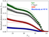Fig. C.1 Normalized photon intensity of the OH(X2Π)(v = 0) intra-ladder mid-IR lines as a function of the rotational number of the upper energy level. The intensities are computed for the fiducial parameters given in Table 1 and for three spectral shapes of the UV field (color coded), and divided by Φ according to Eq. (13). Circle and triangle markers correspond to lines belonging to the Ω = 1∕2 and Ω = 3∕2 ladders, respectively. Λ-doublets are indiscernible in this plot. In this regime, rotational levels are only populated by the radiative cascade of OH photofragments. The solid line is the analytical model assuming that the intra-ladder lines within the v = 0 state are produced by the radiative cascade of OH fragments produced in the v = 0 state (Eq. (C.6)). The dotted line is the analytical model that assumes that any OH produced in a vibrational state instantaneously decays toward the ground vibrational state with a negligible change of its rotational number (see Eq. (C.7)).

The radiative matrix M_ij in Eq. (C.1) can be greatly reduced by noting that the radiative decays of the N levels within the X²Π(v = 0) state are dominated by pure rotational N → N − 1 transitions. Moreover, excited electronic states are found to rapidly decay to the ground electronic state with little change of their vibrational and rotational quantum number. By neglecting the contribution of vibrationally excited levels to the populations of OH(v = 0, N) and assuming that all OH photofragments produced in the OH(A²Σ⁺) (v = 0, N) state decay immediately to the OH(X²Π) (v = 0, N) state, Eq. (C.1) applied to the OH(X)(v = 0, N) levels yields $$A_{N+1\to N}{N}_{N+1}-A_{N\to N-1}{N}_N+\Phi \times \tilde{f}(N,v=0)\simeq 0,$$(C.2)

with $$\tilde{f}(N,v=0)=f(X,N,v=0)+\frac{1}{2}f(A,N,v=0),$$(C.3)

where the factor $\frac{1}{2}$ stands for the different degeneracies between the OH(X)(v, N) and OH(A)(v, N) states. The solution of Eq. (C.2) is then $$A_{N\to N-1}{N}_N\simeq {\tilde{I}}_N\Phi ,$$(C.4)

where $${\tilde{I}}_N\simeq {\sum }_{N^{\prime }\ge N}\tilde{f}(N^{\prime },v=0)$$(C.5)

is the probability to form OH in the ground vibrational state with a rotational number larger than N. The high-N lines are found to be optically thin. Their integrated intensities are then given by 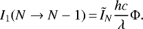$$I_1(N\to N-1)={\tilde{I}}_N\frac{hc}{\lambda }\Phi .$$(C.6)

Thus, according to our analytical model, the normalized integrated photon intensity ${\mathcal{I}}_N$ corresponds to Ĩ_N, the probability to form an OH photofragment in a v = 0 state with a rotational number N′ larger than N. In particular, the line intensities N → N − 1 do not depend on the Einstein-A coefficients. This equation reflects the fact that any OH produced in an excited rotational level N′ will eventually decay through the N → N − 1 transition with N ≤ N′. Because each rotational state of OH is split into two spin-orbit substates that are further subdivided into two Λ-doubling states, Ĩ_N ≤ 1∕4, as seen in Figs. 6 and C.1.

As discussed in Sect. 3.1.1 and further shown in Fig. C.1, our model underestimates the line intensities computed with GROSBETA. This indicates that the radiative decay from vibrationally excited levels contributes to the population of X²Π(N, v = 0) levels. In order to take into account the contribution of vibrationally excited levels, we assume that any OH produced in a vibrationally excited state immediately decays toward the X²Π(v = 0) state with no change of the rotational number. This leads to a normalized integrated photon intensity of 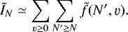$${\tilde{I}}_N\simeq {\sum }_{v\ge 0}{\sum }_{N^{\prime }\ge N}\tilde{f}(N^{\prime },v).$$(C.7)

This model always overestimates the line intensities (dashed lines, Figs. 6 and C.1). This is due to the fact that for N ≳ 15, Einstein-A coefficients of rovibrational transitions are smaller than those of pure rotational transitions. Thus, an OH fragment produced in a v > 0 state tends to decay through the intra-ladder transition within its nascent vibrational state before decaying to the v = 0 state with a lower N number than its nascent one. Below N ≃ 25, the analytical model reproduces well the computed intensities as all levels produced in higher N numbers in v > 0 have decayed toward the v = 0 states. The lines emerging from N < 25 are thus tracing the production of OH in high rotational states, even though the decay of electronically excited OH in the ground vibrational state also contributes to the variation of ${\mathcal{I}}_N$ below N ≃ 25.

Appendix D Conversion factors

Table D.1 gives the line intensities of the OH mid-IR lines in the pure radiative cascade regime normalized by ${\Phi }^{\tilde{B}}$ denoted as ${\mathcal{I}}^{\tilde{B}}$ (see Eq. (18)). The intensity of the N_up → N_up − 1 lines of the OH(X)(v = 0) state are summed over the four components of the quadruplet. ${\mathcal{I}}^{\tilde{B}}$ can be used to convert any line intensity into a column density of H₂O photodissociated per second through the H₂O $\tilde{B}$ state denoted as ${\Phi }^{\tilde{B}}$ using Eq. (20).

Appendix E Critical pumping rate

Figure 7c summarizes the dominant excitation processes as a function of the density n_H and the chemical pumping rate $\mathcal{D}=\Phi /N(\text{OH})$ for a given OH line. The parameter space is split in two regions: For low values of $\mathcal{D}$, the excitation is dominated thermal and radiative processes whereas for high values of $\mathcal{D}$ the excitation is set by the radiative cascade of the OH photofragments.

Fig. E.1 Critical value of the chemical pumping rate ${\mathcal{D}}_{\text{crit}}\equiv {\left(\Phi /N(\text{OH})\right)}_{\text{crit}}$ below which populations in the X2Π(v = 0, N, Ω) states are populated by collisions or IR radiative pumping processes rather than by prompt emission. Collisions or IR radiative pumping are assumed to populate the levels according to a Boltzmann distribution of a single temperature Tex. Because Einstein-A coefficients differ between the two rotational ladders, two ${\mathcal{D}}_{\text{crit}}$ exist for each N quantum number. For simplicity, we have assumed ${\mathcal{I}}_N=0.25$ for all N.

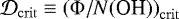
The boundary between the two regions is defined by ${\mathcal{D}}_{\text{crit}}$ (green line Fig. 7c). Its value depends on the physical conditions of the gas, namely n_H, T_IR, and T_K. For example, Fig. 7a shows that ${\mathcal{D}}_{\text{crit}}$ increases from 2 × 10⁻⁹ to 2 × 10⁻⁸ s⁻¹ by increasing the density from n_H = 10⁷ to 10⁹cm⁻³. We propose here to derive simple estimates of ${\mathcal{D}}_{\text{crit}}$ for any rotational level and any T_K and T_IR. To do so, we compare the intensity predicted by a pure radiative cascade (see Eq. (13) and Fig. 6) to that produced bycollisions and/or IR radiative pumping only. In the pure IR radiative pumping regime (regime ②), the line intensity is given by Eq. (14). This yields to a critical chemical pumping rate above which prompt emission sets the population of a level N of $${\mathcal{D}}_{\text{crit}}(T_{\text{ex}},N)=\frac{g_N{A}_{N\to N-1}}{{\mathcal{I}}_{N}Q(T_{\text{ex}})}{e}^{-E_N/k_{\text{B}}{T}_{\text{ex}}},$$(E.1)

where T_ex = T_IR. This equation can also be directly transposed to the high density regime for which T_ex ≃ T_K (regime ④). For intermediate densities, for which both collisions and IR radiative pumping are relevant (regime ③), ${\mathcal{D}}_{\text{crit}}$ varies smoothly from ${\mathcal{D}}_{\text{crit}}(T_{\text{IR}})$ to ${\mathcal{D}}_{\text{crit}}(T_{\text{K}})$ (see Fig. 7c).

Figure E.1 shows ${\mathcal{D}}_{\text{crit}}$ as a function of the upper N number of the level and as a function of the excitation temperature. ${\mathcal{D}}_{\text{crit}}(T_{\text{ex}},N)$ decreases with N, demonstrating that lines with higher N are less sensitive to thermal or radiative excitation processes and more sensitive to prompt emission. This is mostly due to the fact that these lines are coming from levels that are much higher in energy than T_K or T_IR. For higher temperatures, thermal processes are more efficient at populating higher N levels resulting in an increase in ${\mathcal{D}}_{\text{crit}}$. We also note that the decrease in ${\mathcal{D}}_{\text{crit}}$ with N is stiff, showing that for given chemical pumping rate, the transition between lines excited by prompt emission and lines excited by IR radiative pumping or collisions is well defined. In particular, we recover the fact that when collisions are negligible and for T_IR = 120 K, ${\mathcal{D}}_{\text{crit}}\simeq {10}^{-9}$ s⁻¹ for the line coming from N = 10. In contrast, a chemical pumping rate of at least 10⁻⁴ s⁻¹ is required to excite the line coming from N = 6. For high-N levels prompt emission dominates for rates as low as $\mathcal{D}\simeq {10}^{-12}$ s⁻¹. This shows that the schematic view of the parameter space proposed in Fig. 7c remains valid for the low-N lines for which the boundary is shifted to the right, and for high-N lines, for which the boundary is shifted to the left by orders of magnitudes.

References

All Tables

All Figures

Fig. 1 OH model adopted in this work. (a) X2Π and A2 Σ+ electronic levels split into vibrational levels and further split into rotational levels labeled by N (left ladder corresponding the OH(X2Π)(v = 0) state). The red line indicates the dissociation energy of OH(X2Π). (b) Structure of the rotational ladders of OH(X2Π) within a vibrational state that gives rise to mid- and far-IR lines. Each N level is split by the spin-orbit coupling and the Λ-doubling. The two spin-orbit states are labeled by the Ω quantum number and the Λ-doubling states are labeled by their ϵ = e∕f spectroscopic parity. Radiative transitions included in our model and emerging from the four N-levels are also depicted by arrows. There are three kinds of transitions: intra-ladder rotational transitions (blue and red arrows), cross-ladder transitions (green, with ΔN = − 1, and orange, with ΔN = 0, −2), and Λ-doubling transitions (purple). (c) Optically thin LTE spectrum of OH at TK = 750 K. The color code is the same as panel b) and is repeated in Figs. 4 and 9. The upper N level is indicated for some transitions. The Λ-doubling lines are too weak and at longer radio wavelengths to appear in this spectrum. Ro-vibrational lines are at shorter wavelengths than shown here (λ ≲ 2.7 μm).

In the text

Fig. 2 State distribution of the OH product following H2O photodissociation at two photon wavelengths. (a) At λ = 166 nm, H2O dissociating via its first excited à electronic state and producing OH in rotationally cold but vibrationally hot states. (b) At λ = 121.6 nm, H2O dissociating via its second excited $\tilde{B}$ electronic state and producing OH in rotationally hot but vibrationally cold states. Vibrational quantum numbers are color coded as indicated in the top panel. The distributions within OH(X2Π, v) and OH(A2Σ+, v) are plotted in solid and dashed lines, respectively, as a function of the rotational quantum number N. Only vibrational levels that contribute at least 1.5% to the population of nascent OH are shown.

In the text

Fig. 3 Infrared spectra of OH following H2O photodissociation at two photon wavelengths computed with GROSBETA. Top: at λ = 166 nm, H2O dissociating via its first excited à electronic state and producing rotationally cold OH. The OH infrared spectrum is dominated by far-IR lines excited by collisions and IR radiative pumping. Bottom: at λ = 121.6 nm, H2O dissociating via its second excited $\tilde{B}$ electronic state and producing rotationally hot OH. OH lines in the mid-IR with Nup = 20–45 trace H2O photodissociation through this electronic state. The density, temperature of the background radiation and kinetic temperature are fixed to their fiducial values (see Table 1) and Φ = 1010 cm−2 s−1. In this figure, all lines are colored red, even if coming from cross-ladder and intra-ladder transitions.

In the text

Fig. 4 Infrared spectra of OH depending on the column density of H2O photodissociated per unit time Φ and on N(OH) computed with GROSBETA for a Lyα UV radiation field. The density, temperature of the background radiation and kinetic temperature are fixed to their fiducial values (see Table 1). Following the color code used in Fig. 1, intra-ladder rotational lines are in red and blue and cross-ladder lines are in orange and green. Λ-doubling lines are too weak to appear here. The weak mid-IR lines lying in the range ~ 10–13 μm are intra-ladder rotational lines within the OH(X)(v = 1) state. The Nup rotational number of the upper energy level is indicated for selected lines.

In the text

Fig. 5 OH line intensities and the associated excitation processes as a function of Φ and nH for various values of N(OH) and TIR. The color indicates the value of N(OH) and the line style the value of TIR as defined in the right panels. The black circle indicates the fiducial model. The processes that dominate the excitation of the lines depending on the explored parameters are indicated along each curve. Left: intra-ladder rotational line at 10.8 μm coming from a high-N level (N = 30, Eup = 22600 K). This line depends only on Φ. Right: cross-ladder rotational line at 24.6 μm coming from a low-N level (N = 5, Eup = 875 K). This line traces the bulk population of OH. As such, it depends on N(OH), TIR and nH but does not depend on Φ.

In the text

Fig. 6 Normalized photon intensity of the OH(X2Π)(v = 0) intra-ladder mid-IR lines as a function of the quantum number of the upper energy level Nup. The photon intensities are computed for the fiducial values of the parameters and divided by Φ (see Eq. (13)). Circle and triangle markers correspond to lines belonging to the Ω = 1∕2 and Ω = 3∕2 ladders, respectively. Λ-doublets are indiscernible in this plot. In this regime, rotational levels are only populated by the radiative cascade of OH photofragments and ${\mathcal{I}}_{N,\Omega ,ϵ}$, depends only on the spectral shape of the adopted radiation field. The solid line is an analytical model that assumes that the intra-ladder lines within the v = 0 state are powered by the radiative cascade of the OH fragments produced in the v = 0 state. The dotted line is an analytical model that assumes that any OH produced in a vibrational state instantaneously decays toward the ground vibrational state with negligible change in its rotational number (see Appendix C).

In the text

Fig. 7 Transition from prompt emission to thermal or radiative excitation as revealed by the intensity of the intermediate N = 10 rotational line at 27.4 μm. The dominant excitation processes are indicated by ①, ②, ③, ④ as defined in Fig. 5. (a) Line intensity normalized by N(OH) as a function of $\mathcal{D}\equiv \Phi /N(\text{OH})$. The transition between prompt emission and radiative pumping or collisions depends on $\mathcal{D}$ and on nH. In particular, one can define a critical pumping rate ${\mathcal{D}}_{\text{crit}}$ below whichthermal or radiative excitation processes take over from prompt emission. (b) Line intensity normalized by N(OH) as a function of nH for $\mathcal{D}={10}^{-9} {\text{s}}^{-1}<{\mathcal{D}}_{\text{crit}}$. (c) Schematic parameter space indicating the dominant excitation process of the N = 10 line as a function of nH and $\mathcal{D}$. We note that whereas the specific values of $\mathcal{D}$ and nH reported in the x- and y-axis are for the N = 10 line, this schematic view remains valid for any rotational line. The prompt emission region is delimited by ${\mathcal{D}}_{\text{crit}}$ (green line). The regime ① corresponds to the excitation regime of high-N lines whereas the regimes ②, ③ and ④ correspond to the excitation regime of low-N lines. Panels (a) and (b) are cuts in the parameter space and are indicated by red, magenta and blue lines. The temperature of the IR background, the kinetic temperature and the column density of OH are fixed to their fiducial values. The other parameters are indicated in each panel.

In the text

Fig. 8 Rotational distribution of the OH fragments following H2O photodissociation by UV radiation fields of different shapes. The impact of three radiation fields is explored: (a) a radiation field representative of an accreting T Tauri star dominated by a Lyα emission line, (b) an ISRF radiation field and (c) a blackbody radiation field at 10 000 K. Vibrational quantum number are color coded as indicated in the top panel. The distribution is summed over the two electronic states. Only vibrational levels that contribute to at least 1.5% to the population of nascent OH are shown.

In the text

	Fig. 9 OH mid-IR spectrum for various UV spectra computed with GROSBETA for Φ = 1010 cm−2 s−1. Other parameters are constant and equal to their fiducial values given in Table 1. Inthis regime, the intensity of intra-ladder lines (red and blue) are proportional to Φ and do not depend on other parameters such as TIR or nH.
In the text

Fig. 10 Normalized photon intensity of the OH(X2Π)(v = 0) intra-ladder mid-IR lines as a function of the quantum number of the upper energy level Nup. The intensities are computed for the fiducial values of the parameters (see Table 1) and normalized by the column density of water photodissociated via its $\tilde{B}$ state (see Eq. (18)). Circle and triangle markers correspond to lines belonging to the Ω = 1∕2 and Ω = 3∕2 ladders, respectively. Λ-doublets are indiscernible in this plot. In this regime, rotational levels are only populated by the radiative cascade of OH photofragments and ${\mathcal{I}}_{N,\Omega ,ϵ}^{\tilde{B}}$, depends only on the shape of the adopted radiation field.

In the text

Fig. 11 Comparison of the Spitzer-IRS mid-IR spectrum of the tip of HH 211 outflow from Tappe et al. (2008) (black lines) and of a synthetic GROSBETA spectrum for OH (in red) and H2O (in blue). The best fit parameters are indicated in the top right parts of the panels. The GROSBETA spectra are plotted assuming a source size equal to the extraction aperture ΔΩ = 1.9 × 10−9 sr. The rotational quantum number Nup are indicated for some OH lines. The model reproduces well the OH lines at 10–16 μm, but underproduces them at longer wavelengths.

In the text

	Fig. 12 Expected OH mid-IR spectrum at JWST-MIRI resolving power (R ≃ 2000–3000). The parameters of the model correspond to those derived from the Spitzer-IRS observations of HH 211. The weak lines around 9.8 μm are pure rotational lines within the OH(X)(v = 1) state.
In the text

	Fig. A.1 Rotational distributions of nascent OH for various vibrational and electronic states as a function of the photodissociation wavelength. The OH distributions are summed over fine-structure and Λ-doubling states. The difference in the rotational distribution between photodissociation through the à (λ > 143 nm) and $\tilde{B}$ (λ < 143 nm) states of H2O is clearly visible.
In the text

	Fig. A.2 Vibrational distributions of nascent OH for the two electronic states of OH as a function of the UV wavelength. The distributions η are summed over rotational, fine-structure and Λ-doubling states. The difference in the vibrational distribution between photodissociation through the à (λ > 143 nm) and $\tilde{B}$ (λ < 143 nm) states of H2O is clearly visible.
In the text

Fig. A.3 Radiation fields and H2O photodissociation cross section adopted in this work. Top: spectral shape of the radiation fields as a function of wavelength. The radiation fields have been scaled to agree with the integrated energy-intensity of the Draine (1978) radiation field between 91.2 and 200 nm, that is, 2.6 × 10−6 W m−2. Bottom: photodissociation cross section of H2O producing OH adopted in this work (black) and the extension to 911 Å (gray). The features due to photodissociation through the Ã, $\tilde{B}$, $\tilde{C}$, and $\tilde{D}$ states of H2O are also indicated.

In the text

Fig. C.1 Normalized photon intensity of the OH(X2Π)(v = 0) intra-ladder mid-IR lines as a function of the rotational number of the upper energy level. The intensities are computed for the fiducial parameters given in Table 1 and for three spectral shapes of the UV field (color coded), and divided by Φ according to Eq. (13). Circle and triangle markers correspond to lines belonging to the Ω = 1∕2 and Ω = 3∕2 ladders, respectively. Λ-doublets are indiscernible in this plot. In this regime, rotational levels are only populated by the radiative cascade of OH photofragments. The solid line is the analytical model assuming that the intra-ladder lines within the v = 0 state are produced by the radiative cascade of OH fragments produced in the v = 0 state (Eq. (C.6)). The dotted line is the analytical model that assumes that any OH produced in a vibrational state instantaneously decays toward the ground vibrational state with a negligible change of its rotational number (see Eq. (C.7)).

In the text

Fig. E.1 Critical value of the chemical pumping rate ${\mathcal{D}}_{\text{crit}}\equiv {\left(\Phi /N(\text{OH})\right)}_{\text{crit}}$ below which populations in the X2Π(v = 0, N, Ω) states are populated by collisions or IR radiative pumping processes rather than by prompt emission. Collisions or IR radiative pumping are assumed to populate the levels according to a Boltzmann distribution of a single temperature Tex. Because Einstein-A coefficients differ between the two rotational ladders, two ${\mathcal{D}}_{\text{crit}}$ exist for each N quantum number. For simplicity, we have assumed ${\mathcal{I}}_N=0.25$ for all N.

In the text

References

- Beenakker, C. I. M., Heer, F. J. D., Krop, H. B., & Möhlmann, G. R. 1974, Chem. Phys., 6, 445 [CrossRef] [Google Scholar]
- Benz, A. O., Bruderer, S., van Dishoeck, E. F., et al. 2016, A&A, 590, A105 [NASA ADS] [CrossRef] [EDP Sciences] [Google Scholar]
- Bergin, E., Calvet, N., D’Alessio, P., & Herczeg, G. J. 2003, ApJ, 591, L159 [Google Scholar]
- Bergin, E. A., Du, F., Cleeves, L. I., et al. 2016, ApJ, 831, 101 [NASA ADS] [CrossRef] [Google Scholar]
- Black, J. H. 1998, Faraday Discuss., 109, 257 [NASA ADS] [CrossRef] [Google Scholar]
- Black, J. H., & van Dishoeck, E. F. 1987, ApJ, 322, 412 [NASA ADS] [CrossRef] [Google Scholar]
- Bodewits, D., Országh, J., Noonan, J., Ďurian, M., & Matejčík, Š. 2019, ApJ, 885, 167 [CrossRef] [Google Scholar]
- Boogert, A. C. A., Gerakines, P. A., & Whittet, D. C. B. 2015, ARA&A, 53, 541 [Google Scholar]
- Brooke, J. S. A., Bernath, P. F., Western, C. M., et al. 2016, J. Quant. Spec. Radiat. Transf., 168, 142 [NASA ADS] [CrossRef] [Google Scholar]
- Bruderer, S., van Dishoeck, E. F., Doty, S. D., & Herczeg, G. J. 2012, A&A, 541, A91 [NASA ADS] [CrossRef] [EDP Sciences] [Google Scholar]
- Carr, J. S., & Najita, J. R. 2011, ApJ, 733, 102 [Google Scholar]
- Carr, J. S., & Najita, J. R. 2014, ApJ, 788, 66 [NASA ADS] [CrossRef] [Google Scholar]
- Cazzoletti, P., van Dishoeck, E. F., Visser, R., Facchini, S., & Bruderer, S. 2018, A&A, 609, A93 [NASA ADS] [CrossRef] [EDP Sciences] [Google Scholar]
- Ceccarelli, C., Hollenbach, D. J., & Tielens, A. G. G. M. 1996, ApJ, 471, 400 [Google Scholar]
- Chang, Y., Yu, Y., Wang, H., et al. 2019, Nat. Commun., 10, 1250 [CrossRef] [Google Scholar]
- Chapman, N. L., Mundy, L. G., Lai, S.-P., & Evans, Neal, J., I. 2009, ApJ, 690, 496 [NASA ADS] [CrossRef] [Google Scholar]
- Chokshi, A., Tielens, A. G. G. M., & Hollenbach, D. 1993, ApJ, 407, 806 [Google Scholar]
- Chyba, C. F., & Hand, K. P. 2005, ARA&A, 43, 31 [Google Scholar]
- Coppola, C. M., Galli, D., Palla, F., Longo, S., & Chluba, J. 2013, MNRAS, 434, 114 [CrossRef] [Google Scholar]
- Cuppen, H. M., & Herbst, E. 2007, ApJ, 668, 294 [Google Scholar]
- Dionatos, O., Ray, T., & Güdel, M. 2018, A&A, 616, A84 [CrossRef] [EDP Sciences] [Google Scholar]
- Dobbyn, A. J., & Knowles, P. J. 1997, Mol. Phys., 91, 1107 [NASA ADS] [Google Scholar]
- Dopita, M. A., & Sutherland, R. S. 2017, ApJS, 229, 35 [NASA ADS] [CrossRef] [Google Scholar]
- Draine, B. T. 1978, ApJS, 36, 595 [NASA ADS] [CrossRef] [Google Scholar]
- Fedele, D., Pascucci, I., Brittain, S., et al. 2011, ApJ, 732, 106 [Google Scholar]
- Fillion, J. H., van Harrevelt, R., Ruiz, J., et al. 2001, J. Phys. Chem. A, 105, 11414 [CrossRef] [Google Scholar]
- Fillion, J. H., Dulieu, F., Baouche, S., et al. 2003, J. Phys. B At. Mol. Phys., 36, 2767 [NASA ADS] [CrossRef] [Google Scholar]
- Fillion, J. H., Ruiz, J., Yang, X. F., et al. 2004, J. Chem. Phys., 120, 6531 [NASA ADS] [CrossRef] [Google Scholar]
- Flagey, N., Goldsmith, P. F., Lis, D. C., et al. 2013, ApJ, 762, 11 [Google Scholar]
- Flower, D. R. & Pineau des Forêts, G. 2012, MNRAS, 421, 2786 [NASA ADS] [CrossRef] [Google Scholar]
- Gammie, C. F. 1996, ApJ, 457, 355 [NASA ADS] [CrossRef] [Google Scholar]
- Godard, B., & Cernicharo, J. 2013, A&A, 550, A8 [NASA ADS] [CrossRef] [EDP Sciences] [Google Scholar]
- Godard, B., Pineau des Forêts, G., Lesaffre, P., et al. 2019, A&A, 622, A100 [NASA ADS] [CrossRef] [EDP Sciences] [Google Scholar]
- Goicoechea, J. R., Joblin, C., Contursi, A., et al. 2011, A&A, 530, L16 [NASA ADS] [CrossRef] [EDP Sciences] [Google Scholar]
- Goicoechea, J. R., Cernicharo, J., Karska, A., et al. 2012, A&A, 548, A77 [NASA ADS] [CrossRef] [EDP Sciences] [Google Scholar]
- Goicoechea, J. R., Chavarría, L., Cernicharo, J., et al. 2015, ApJ, 799, 102 [Google Scholar]
- González-Alfonso, E., Fischer, J., Graciá-Carpio, J., et al. 2012, A&A, 541, A4 [NASA ADS] [CrossRef] [EDP Sciences] [Google Scholar]
- Gorti, U., & Hollenbach, D. 2004, ApJ, 613, 424 [NASA ADS] [CrossRef] [Google Scholar]
- Gorti, U., Hollenbach, D., Najita, J., & Pascucci, I. 2011, ApJ, 735, 90 [NASA ADS] [CrossRef] [Google Scholar]
- Habing, H. J. 1968, Bull. Astron. Inst. Netherlands, 19, 421 [Google Scholar]
- Harich, S. A., Hwang, D. W. H., Yang, X., et al. 2000, J. Chem. Phys., 113, 10073 [CrossRef] [Google Scholar]
- Harsono, D., Persson, M. V., Ramos, A., et al. 2020, A&A, 636, A26 [CrossRef] [EDP Sciences] [Google Scholar]
- Heays, A. N., Bosman, A. D., & van Dishoeck, E. F. 2017, A&A, 602, A105 [NASA ADS] [CrossRef] [EDP Sciences] [Google Scholar]
- Hensley, B. S., & Draine, B. T. 2020, ApJ, 895, 38 [CrossRef] [Google Scholar]
- Herczeg, G. J., Wood, B. E., Linsky, J. L., Valenti, J. A., & Johns-Krull, C. M. 2004, ApJ, 607, 369 [NASA ADS] [CrossRef] [Google Scholar]
- Hirano, N., Liu, S.-Y., Shang, H., et al. 2006, ApJ, 636, L141 [Google Scholar]
- Hollenbach, D., & McKee, C. F. 1989, ApJ, 342, 306 [NASA ADS] [CrossRef] [Google Scholar]
- Hwang, D. W., Yang, X., & Yang, X. 1999a, J. Chem. Phys., 110, 4119 [CrossRef] [Google Scholar]
- Hwang, D. W., Yang, X. F., Harich, S., Lin, J. J., & Yang, X. 1999b, J. Chem. Phys., 110, 4123 [CrossRef] [Google Scholar]
- Jørgensen, J. K., & van Dishoeck, E. F. 2010, ApJ, 710, L72 [NASA ADS] [CrossRef] [Google Scholar]
- Karska, A., Herczeg, G. J., van Dishoeck, E. F., et al. 2013, A&A, 552, A141 [NASA ADS] [CrossRef] [EDP Sciences] [Google Scholar]
- Karska, A., Kristensen, L. E., van Dishoeck, E. F., et al. 2014, A&A, 572, A9 [NASA ADS] [CrossRef] [EDP Sciences] [Google Scholar]
- Kłos, J., Lique, F., & Alexander, M. H. 2007, Chem. Phys. Lett., 445, 12 [NASA ADS] [CrossRef] [Google Scholar]
- Kristensen, L. E., van Dishoeck, E. F., Bergin, E. A., et al. 2012, A&A, 542, A8 [NASA ADS] [CrossRef] [EDP Sciences] [Google Scholar]
- Kristensen, L. E., van Dishoeck, E. F., Mottram, J. C., et al. 2017, A&A, 605, A93 [NASA ADS] [CrossRef] [EDP Sciences] [Google Scholar]
- Krotkov, R., Wang, D., & Scoville, N. Z. 1980, ApJ, 240, 940 [NASA ADS] [CrossRef] [Google Scholar]
- Lehmann, A., Godard, B., Pineau des Forêts, G., & Falgarone, E. 2020, A&A, 643, A101 [EDP Sciences] [Google Scholar]
- Liu, X., Lin, J. J., Harich, S., Schatz, G. C., & Yang, X. 2000, Science, 289, 1536 [CrossRef] [Google Scholar]
- Mathis, J. S., Mezger, P. G., & Panagia, N. 1983, A&A, 500, 259 [NASA ADS] [Google Scholar]
- McClure, M. 2009, ApJ, 693, L81 [NASA ADS] [CrossRef] [Google Scholar]
- Melnick, G. J., & Kaufman, M. J. 2015, ApJ, 806, 227 [Google Scholar]
- Mota, R., Parafita, R., Giuliani, A., et al. 2005, Chem. Phys. Lett., 416, 152 [NASA ADS] [CrossRef] [Google Scholar]
- Neufeld, D. A., & Dalgarno, A. 1989, ApJ, 340, 869 [Google Scholar]
- Neufeld, D. A., Lepp, S., & Melnick, G. J. 1995, ApJS, 100, 132 [NASA ADS] [CrossRef] [Google Scholar]
- Nisini, B., Giannini, T., & Lorenzetti, D. 2002, ApJ, 574, 246 [Google Scholar]
- Nisini, B., Santangelo, G., Antoniucci, S., et al. 2013, A&A, 549, A16 [NASA ADS] [CrossRef] [EDP Sciences] [Google Scholar]
- Offer, A. R., van Hemert, M. C., & van Dishoeck, E. F. 1994, J. Chem. Phys., 100, 362 [NASA ADS] [CrossRef] [Google Scholar]
- Panoglou, D., Cabrit, S., Pineau Des Forêts, G., et al. 2012, A&A, 538, A2 [NASA ADS] [CrossRef] [EDP Sciences] [Google Scholar]
- Parikka, A., Habart, E., Bernard-Salas, J., et al. 2017, A&A, 599, A20 [NASA ADS] [CrossRef] [EDP Sciences] [Google Scholar]
- Persson, M. V., Jørgensen, J. K., & van Dishoeck, E. F. 2012, A&A, 541, A39 [NASA ADS] [CrossRef] [EDP Sciences] [Google Scholar]
- Persson, M. V., Harsono, D., Tobin, J. J., et al. 2016, A&A, 590, A33 [NASA ADS] [CrossRef] [EDP Sciences] [Google Scholar]
- Pontoppidan, K. M., Salyk, C., Blake, G. A., et al. 2010, ApJ, 720, 887 [Google Scholar]
- Pontoppidan, K. M., Salyk, C., Bergin, E. A., et al. 2014, in Protostars and Planets VI, eds. H. Beuther, R. S. Klessen, C. P. Dullemond, & T. Henning, 363 [Google Scholar]
- Raymond, J. C. 1979, ApJS, 39, 1 [NASA ADS] [CrossRef] [Google Scholar]
- Rieke, G. H., Wright, G. S., Böker, T., et al. 2015, PASP, 127, 584 [NASA ADS] [CrossRef] [Google Scholar]
- Röllig, M., Abel, N. P., Bell, T., et al. 2007, A&A, 467, 187 [NASA ADS] [CrossRef] [EDP Sciences] [Google Scholar]
- Salyk, C., Pontoppidan, K. M., Blake, G. A., Najita, J. R., & Carr, J. S. 2011, ApJ, 731, 130 [NASA ADS] [CrossRef] [Google Scholar]
- Schindhelm, E., France, K., Herczeg, G. J., et al. 2012, ApJ, 756, L23 [NASA ADS] [CrossRef] [Google Scholar]
- Schoonenberg,D., & Ormel, C. W. 2017, A&A, 602, A21 [NASA ADS] [CrossRef] [EDP Sciences] [Google Scholar]
- Slanger, T. G., & Black, G. 1982, J. Chem. Phys., 77, 2432 [NASA ADS] [CrossRef] [Google Scholar]
- Stäuber, P., & Bruderer, S. 2009, A&A, 505, 195 [NASA ADS] [CrossRef] [EDP Sciences] [Google Scholar]
- Sturm, E., González-Alfonso, E., Veilleux, S., et al. 2011, ApJ, 733, L16 [Google Scholar]
- Tabone, B., Godard, B., Pineau des Forêts, G., Cabrit, S., & van Dishoeck, E. F. 2020, A&A, 636, A60 [CrossRef] [EDP Sciences] [Google Scholar]
- Tappe, A., Lada, C. J., Black, J. H., & Muench, A. A. 2008, ApJ, 680, L117 [Google Scholar]
- Tappe, A., Forbrich, J., Martín, S., Yuan, Y., & Lada, C. J. 2012, ApJ, 751, 9 [NASA ADS] [CrossRef] [Google Scholar]
- Tennyson, J., Yurchenko, S. N., Al-Refaie, A. F., et al. 2016, J. Mol. Spectr., 327, 73 [NASA ADS] [CrossRef] [Google Scholar]
- Testi, L., Birnstiel, T., Ricci, L., et al. 2014, in Protostars and Planets VI, eds. H. Beuther, R. S. Klessen, C. P. Dullemond, & T. Henning, 339 [Google Scholar]
- Thi, W. F., Kamp, I., Woitke, P., et al. 2013, A&A, 551, A49 [NASA ADS] [CrossRef] [EDP Sciences] [Google Scholar]
- van der Tak, F. F. S., Black, J. H., Schöier, F. L., Jansen, D. J., & van Dishoeck, E. F. 2007, A&A, 468, 627 [NASA ADS] [CrossRef] [EDP Sciences] [Google Scholar]
- van Dishoeck, E. F., & Dalgarno, A. 1983, J. Chem. Phys., 79, 873 [NASA ADS] [CrossRef] [Google Scholar]
- van Dishoeck, E. F., Jonkheid, B., & van Hemert, M. C. 2006, Faraday Discuss., 133, 231 [Google Scholar]
- van Dishoeck, E. F., Kristensen, L. E., Benz, A. O., et al. 2011, PASP, 123, 138 [Google Scholar]
- van Dishoeck, E. F., Bergin, E. A., Lis, D. C., & Lunine, J. I. 2014, in Protostars and Planets VI, eds. H. Beuther, R. S. Klessen, C. P. Dullemond, & T. Henning, 835 [Google Scholar]
- van Harrevelt, R., & van Hemert, M. C. 2000, J. Chem. Phys., 112, 5787 [NASA ADS] [CrossRef] [Google Scholar]
- van Harrevelt, R., & van Hemert, M. C. 2001, J. Chem. Phys., 114, 9453 [NASA ADS] [CrossRef] [Google Scholar]
- van Harrevelt, R., & van Hemert, M. C. 2008, J. Phys. Chem. A, 112, 3002 [CrossRef] [Google Scholar]
- van Kempen, T. A., Kristensen, L. E., Herczeg, G. J., et al. 2010, A&A, 518, L121 [NASA ADS] [CrossRef] [EDP Sciences] [Google Scholar]
- van ’t Hoff, M. L. R., van Dishoeck, E. F., Jørgensen, J. K., & Calcutt, H. 2020, A&A, 633, A7 [CrossRef] [EDP Sciences] [Google Scholar]
- Visser, R., van Dishoeck, E. F., Doty, S. D., & Dullemond, C. P. 2009, A&A, 495, 881 [NASA ADS] [CrossRef] [EDP Sciences] [Google Scholar]
- Visser, R., Kristensen, L. E., Bruderer, S., et al. 2012, A&A, 537, A55 [NASA ADS] [CrossRef] [EDP Sciences] [Google Scholar]
- Visser, R., Jørgensen, J. K., Kristensen, L. E., van Dishoeck, E. F., & Bergin, E. A. 2013, ApJ, 769, 19 [Google Scholar]
- Walawender, J., Bally, J., Kirk, H., et al. 2006, AJ, 132, 467 [NASA ADS] [CrossRef] [Google Scholar]
- Walsh, C., Nomura, H., Millar, T. J., & Aikawa, Y. 2012, ApJ, 747, 114 [Google Scholar]
- Walsh, C., Nomura, H., & van Dishoeck, E. 2015, A&A, 582, A88 [NASA ADS] [CrossRef] [EDP Sciences] [Google Scholar]
- Wampfler, S. F., Herczeg, G. J., Bruderer, S., et al. 2010, A&A, 521, L36 [NASA ADS] [CrossRef] [EDP Sciences] [Google Scholar]
- Wampfler, S. F., Bruderer, S., Kristensen, L. E., et al. 2011, A&A, 531, L16 [NASA ADS] [CrossRef] [EDP Sciences] [Google Scholar]
- Wampfler, S. F., Bruderer, S., Karska, A., et al. 2013, A&A, 552, A56 [NASA ADS] [CrossRef] [EDP Sciences] [Google Scholar]
- Wang, L., Bai,X.-N., & Goodman, J. 2019, ApJ, 874, 90 [NASA ADS] [CrossRef] [Google Scholar]
- Woitke, P., Min, M., Pinte, C., et al. 2016, A&A, 586, A103 [NASA ADS] [CrossRef] [EDP Sciences] [Google Scholar]
- Wright, G. S., Wright, D., Goodson, G. B., et al. 2015, PASP, 127, 595 [Google Scholar]
- Yang, X. F., Hwang, D. W., Lin, J. J., & Ying, X. 2000, J. Chem. Phys., 113, 10597 [CrossRef] [Google Scholar]
- Yang, H., Herczeg, G. J., Linsky, J. L., et al. 2012, ApJ, 744, 121 [NASA ADS] [CrossRef] [Google Scholar]
- Yarkony, D. R. 1992, J. Chem. Phys., 97, 1838 [NASA ADS] [CrossRef] [Google Scholar]
- Yousefi, M., Bernath, P. F., Hodges, J., & Masseron, T. 2018, J. Quant. Spec. Radiat. Transf., 217, 416 [CrossRef] [Google Scholar]
- Yvart, W., Cabrit, S., Pineau des Forêts, G., & Ferreira, J. 2016, A&A, 585, A74 [NASA ADS] [CrossRef] [EDP Sciences] [Google Scholar]
- Zhou, L., Xie, D., & Guo, H. 2015, J. Chem. Phys., 142, 124317 [CrossRef] [Google Scholar]
The spectroscopic parity index is related to the parity p = + ∕− by the relation  , where ϵ = 1 for e states and ϵ = − 1 for f states.
is the probability of OH in a given state to be destroyed [in s−1]. Consequently, this assumption leads to
and not
, with n the number of OH levels included in the model, as stated in Stäuber & Bruderer (2009).
In the case of the photodissociation by a Lyα
radiation field studied in Sect. 3.1,  and
and  .
.
All Tables
Branching ratio between H2O photodissociation leading to OH through the à state (λ ≳ 143 nm) and the state (114 ≲ λ ≲ 143 nm) for UV radiation fields of various spectral shapes.
Conversion factors between the photon intensity integrated over solid angle (in photon cm−2 s−1) of the rotational lines Nup → Nup − 1 summed over the components of each quadruplet and (molecule cm−2 s−1).