| Issue |
A&A
Volume 649, May 2021
|
|
|---|---|---|
| Article Number | A90 | |
| Number of page(s) | 10 | |
| Section | Planets and planetary systems | |
| DOI | https://doi.org/10.1051/0004-6361/202039817 | |
| Published online | 18 May 2021 | |
KMT-2018-BLG-1025Lb: microlensing super-Earth planet orbiting a low-mass star★
1
Department of Physics, Chungbuk National University,
Cheongju
28644,
Republic of Korea
e-mail: This email address is being protected from spambots. You need JavaScript enabled to view it.
2
Astronomical Observatory, University of Warsaw,
Al. Ujazdowskie 4,
00-478
Warszawa,
Poland
3
Korea Astronomy and Space Science Institute,
Daejon
34055,
Republic of Korea
4
University of Canterbury, Department of Physics and Astronomy,
Private Bag 4800,
Christchurch
8020,
New Zealand
5
Korea University of Science and Technology,
217 Gajeong-ro,
Yuseong-gu,
Daejeon
34113,
Republic of Korea
6
Max Planck Institute for Astronomy,
Königstuhl 17,
69117
Heidelberg,
Germany
7
Department of Astronomy, The Ohio State University,
140 W. 18th Ave.,
Columbus,
OH
43210,
USA
8
Department of Particle Physics and Astrophysics, Weizmann Institute of Science,
Rehovot
76100,
Israel
9
Center for Astrophysics, Harvard & Smithsonian 60 Garden St.,
Cambridge,
MA
02138,
USA
10
Department of Astronomy and Tsinghua Centre for Astrophysics, Tsinghua University,
Beijing
100084,
PR China
11
School of Space Research, Kyung Hee University,
Yongin,
Kyeonggi
17104,
Republic of Korea
12
Department of Astronomy & Space Science, Chungbuk National University,
Cheongju
28644,
Republic of Korea
13
Department of Physics & Astronomy, Seoul National University,
Seoul
08826,
Republic of Korea
14
Division of Physics, Mathematics, and Astronomy, California Institute of Technology,
Pasadena,
CA
91125,
USA
15
Department of Physics, University of Warwick,
Gibbet Hill Road,
Coventry,
CV4 7AL,
UK
Received:
31
October
2020
Accepted:
3
February
2021
Abstract
Aims. We aim to find missing microlensing planets hidden in the unanalyzed lensing events of previous survey data.
Methods. For this purpose, we conducted a systematic inspection of high-magnification microlensing events, with peak magnifications of Apeak ≳ 30, in the data collected from high-cadence surveys in and before the 2018 season. From this investigation, we identified an anomaly in the lensing light curve of the event KMT-2018-BLG-1025. The analysis of the light curve indicates that the anomaly is caused by a very low mass-ratio companion to the lens.
Results. We identify three degenerate solutions, in which the ambiguity between a pair of solutions (solutions B) is caused by the previously known close–wide degeneracy, and the degeneracy between these and the other solution (solution A) is a new type that has not been reported before. The estimated mass ratio between the planet and host is q ~ 0.8 × 10⁻⁴ for solution A and q ~ 1.6 × 10⁻⁴ for solutions B. From the Bayesian analysis conducted with measured observables, we estimate that the masses of the planet and host and the distance to the lens are (Mp, Mh, DL) ~ (6.1 M⊕, 0.22 M⊙, 6.7 kpc) for solution A and ~(4.4 M⊕, 0.08 M⊙, 7.5 kpc) for solutions B. The planet mass is in the category of a super-Earth regardless of the solutions, making the planet the eleventh super-Earth planet, with masses lying between those of Earth and the Solar System’s ice giants, which were discovered by microlensing.
Key words: gravitational lensing: micro / planets and satellites: general
Photometric data are only available at the CDS via anonymous ftp to cdsarc.u-strasbg.fr (130.79.128.5) or via http://cdsarc.u-strasbg.fr/viz-bin/cat/J/A+A/649/A90
© ESO 2021
1 Introduction
The microlensing method has unique advantages in detecting some specific populations of planets. It enables one to detect planets orbiting very faint low-mass stars, which are the most common populations of stars in the Galaxy, because of the lensing characteristic that does not depend on the luminosity of the planet host. Another very important advantage of the method is that its detection efficiency extends to very low-mass planets because of the slow decrease in the efficiency with the decrease in the planet/host mass ratio q. The microlensing efficiency decreases as  , while the efficiency of other methods, for example, the radial-velocity method, decreases in direct proportion to q (see Gaudi 2012 for a review on various advantages of the microlensing method). With a sensitivity to planets that are difficult to be detected by other methods, microlensing plays an important role to complement other methods not only for the complete demographic census of planets but also for the comprehensive understanding of the planet formation process.
However, these advantages of the microlensing method, especially the latter one, that is to say the high sensitivity to low-mass planets, were difficult to be fully realized during the early generation of microlensing experiments, for example MACHO (Alcock et al 1997) and OGLE (Udalski et al. 1994). A planetary microlensing signal, in general, appears as a short-term anomaly to the smooth and symmetric lensing light curve generated by the host of the planet (Mao & Paczyński 1991; Gould & Loeb 1992). For this reason, a microlensing planet search should be carried out in two steps: first by detecting lensing events, and second by inspecting planet-induced anomalies in the light curves of detected lensing events. The probability for a star to be gravitationally lensed is very low, on the order of 10−6 for stars located in the Galactic bulge field, toward which microlensing surveys have been and are being carried out (Paczyński 1991; Griest et al. 1991; Sumi & Penny 2016; Mróz et al. 2019), and thus a lensing survey should cover a large area of sky to increase the number of lensing events by maximizing the number of monitored stars. This requirement had limited the cadence of lensing surveys and subsequently the rate of planet detections, especially that of very low-mass planets. Gould & Loeb (1992) proposed to overcome this problem by conducting intensive follow-up observations of survey-detected events, which led to the first detections of low-mass planets (Beaulieu et al. 2006; Gould et al. 2006). However, this approach is restricted to a small number of events due to telescope resources.
The planet detection rate has rapidly increased with the operation of high-cadence lensing surveys including MOA II (Bond et al. 2001), OGLE-IV (Udalski et al. 2015), and KMTNet (Kim et al. 2016). By employing multiple telescopes equipped with large-formatcameras, these surveys achieve an observation cadence reaching down to 15 min for dense bulge fields. This cadence is shorter than those of the first-generation MACHO and OGLE surveys, which had been carried out with a ~ 1 day cadence, by about a factor of 100.
The great shortening of the observation cadence resulted in a rapid increase in the planet detection rate. The population of planets with a remarkable increase in the detection rate is super-Earth planets, which are defined as planets having masses higher than the mass of Earth, but substantially lower than those of the Solar System’s ice giants, Uranus and Neptune (Valencia et al. 2007)1. In Table 1, we list the microlensing super-Earth planets, along with the masses of the planets and their hosts, which have been detected from the last 28 yr-long operation of lensing surveys since 1992. Among the total ten super-Earth planets, seven were detected during the last four years since the full operation of the KMTNet survey in 2016, and for all of these events, the KMTNet data played key roles in detecting and characterizing the planets.
In this paper, we report the detection of a new microlensing super-Earth planet. The planet was found from a project thatwas conducted to search for unrecognized planets in the previous KMTNet data collected in and before the 2018 season. In the first part of this project, Han et al. (2020b) investigated lensing events with faint source stars, considering the possibility that planetary signals might be missed due to the noise or scatter of data. From the investigation, they found four planetary events that had not been reported before. The new planetary system that we report in this work was found in the second part of the project that was carried out by inspecting subtle planetary signals in the light curves of high-magnification lensing events with peak magnifications of Apeak ≳ 30. In this project,high-magnification events were selected as targets for reinspection because the sensitivity to planets for these events is high (Griest & Safizadeh 1998). Despite the high chance of planet perturbations, some planetary signals produced by a non-caustic-crossing channel may not be noticed due to their weak signals (Zhu et al. 2014).
For the presentation of the work, we organize the paper as follows. The acquisition and reduction processes of the data used in the analysis are discussed in Sect. 2. We describe the characteristics of the anomaly in the lensing light curve in Sect. 3. We explain various models tested to explain the observed anomaly and show that the anomaly is of a planetary origin in Sect. 4. The procedure to estimate the angular Einstein radius is discussed in Sect. 5. We estimate the physical parameters of the planetary system, including the mass and distance, in Sect. 6. We summarize the results and conclude in Sect. 7.
Microlensing super-Earth planets.
2 Observations and data
The planet was found from the analysis of the microlensing event KMT-2018-BLG-1075. The source star of the event lies in the Galactic bulge field with the equatorial coordinates of (RA, Dec) = (17 : 59 : 27.94, −27 : 52 : 41.02), which correspond to the Galactic coordinates of (l, b) = (2°.461, −2°.082). The flux from the source, which had been constant before the lensing-induced magnification with an apparent baseline brightness of I ~ 19.65, was highly magnified for about 10 days centered at HJD′≡HJD − 2 450 000 ~ 8274.85. The event was found from the post-season inspection of the 2018 season data using the KMTNet Event Finder System (Kim et al. 2018). At the time of finding, the event drew little attention due to the similarity of the lensing light curve to that of a regular single-source single-lens (1L1S) event (see more detailed discussion in the following section).
Observations of the event by the KMTNet survey were conducted using three telescopes that are located in Australia (KMTA), Chile (KMTC), and South Africa (KMTS). Each telescope has a 1.6m aperture and is equipped with a camera yielding 4 deg2 field of view. The event is located in the two overlapping survey fields of “BLG03” and “BLG43,” which are displaced with a slight offset to fill the gaps between the chips of the camera. Observations in each field were conducted with a 30 min cadence, resulting in a combined cadence of 15 min. Thanks to the high-cadence coverage of the event using the globally distributed multiple telescopes, the peak region of the event was continuously and densely covered.
Images of the source were mostly obtained in the I band, and a fraction of images were acquired in the V band for themeasurement of the source color. Reduction of the data was done using the KMTNet pipeline (Albrow et al. 2009) based on the difference imaging method (Tomaney & Crotts 1996; Alard & Lupton 1998), which was developed for the optimal photometry of stars lying in very dense star fields. For a subset of the KMTC data, additional photometry was conducted using the pyDIA software (Albrow 2017) to construct a color-magnitude diagram (CMD) of stars and to measure the color of the source star. The detailed procedure of determining the source color is described in Sect. 5. Error bars of the data estimated from the automatized photometric pipeline were readjusted using the method of Yee et al. (2012). In this method, the error bars are renormalized by ![Mathematical equation: $\sigma=[\sigma_{\textrm{min}}^2 + (k\sigma_0)^2]^{1/2}$](/articles/aa/full_html/2021/05/aa39817-20/aa39817-20-eq2.png) , where σ0 denotes the error estimated from the pipeline, σmin is a scatter of data, and k is a factor used to make χ2 per degree of freedom (dof) unity. In Table 2, we list the numbers and the data readjustment factors for the individual data sets.
, where σ0 denotes the error estimated from the pipeline, σmin is a scatter of data, and k is a factor used to make χ2 per degree of freedom (dof) unity. In Table 2, we list the numbers and the data readjustment factors for the individual data sets.
Although the lensing event was not found at the time of the lensing magnification, the source star of the event lies in the field covered by the OGLE survey. We, therefore, checked the OGLE images containing the source and conducted photometry for the source identified by the KMTNet survey. From this, we recovered the OGLE photometry data, among which seven data points cover the peak of the light curve. OGLE observations were done using the 1.3m telescope of the Las Campanas Observatory in Chile, and reduction was carried out using the OGLE photometry pipeline (Udalski 2003). We have published the photometry data to ensure reproducibility of the analysis2.
Data readjustment factors.
3 Characteristics of the anomaly
The light curve of KMT-2018-BLG-1025 is shown in Fig. 1. At first glance, it appears to have a smooth and symmetric form of a 1L1S event. A 1L1S modeling yields an impact parameter (scaled to the angular Einstein radius θE) of the lens-source approach and an event timescale of (u0, tE) ~ (0.0064, 10.1 days), respectively,indicating that the event has a relatively short timescale with a high peak magnification of Apeak ~ 1∕u0 ~ 150. The 1L1S model curve is plotted over the data points in Fig. 1. The full lensing parameters and their uncertainties are listed in Table 3, where t0 indicates the time of the closest lens-source approach. We note that finite-source effects are considered in the 1L1S model, but the effects are negligible, and thus the value of the normalized source radius ρ is not presented in the table. The normalized source radius is defined as the ratio of the angular source radius θ* to θE, that is, ρ = θ*∕θE.
The event was reanalyzed because it was selected in the list of high-magnification events for close examinations among the KMTNet events detected in and before the 2018 season in search for planetary signals that had not been noticed previously. From this analysis, we find that the light curve exhibits a subtle but noticeable deviation from a 1L1S model.
In the lower two panels of Fig. 1, we present a zoomed-in view of the light curve and residuals from the 1L1S model in the peak region, which shows a slight bump in the residuals centered at t1 ~ 8274.38 and a dip centered at t2 ~ 8274.66. Although minor, with ΔI ≲ 0.05 magnitude, the deviation drew our attention for two major reasons. The first reason is that the deviation occurred in the central magnification region, in which the chance of a planet-induced perturbation is high (Griest & Safizadeh 1998). The second reason is that different data sets exhibit a consistent pattern of deviation. The data sets obtained using the KMTC telescope, located in Chile, and the KMTS telescope, located in South Africa, show consistent deviations. Considering that the two telescopes are remotely located, it is difficult to explain the consistency with coincidental systematics in the data such as changes in transparency. Furthermore, the OGLE data in the deviation region exhibit a consistent anomaly pattern with that of the KMTC data, although their coverage is not very dense. Therefore, the deviation is very likely to be real.
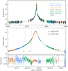 |
Fig. 1 Light curve of KMT-2018-BLG-1025. Upper and lower panels: whole view and the zoomed-in view of the peak region, respectively. The colors of data points indicate the observatories, as given in the legend. The curve plotted over the data points is the 1L1S model, for which the residuals in the peak region are presented in the bottom panel. The dotted vertical lines at t1 ~ 8274.38 and t2 ~8274.66 indicate the respective times of the bump and dip in the residuals to the 1L1S model. |
Lensing parameters of various tested models.
4 Interpretation of the anomaly
The fact that the anomaly occurred in the peak region of a high-magnification event suggests the possibility that the anomaly may be produced by a planetary companion, M2, to the primary lens, M1. In order to check this possibility, we conducted an additional modeling under a binary-lens (2L1S) interpretation.
The modeling was carried out to find a set of lensing parameters that best explain the observed anomaly in the light curve. In addition to the 1L1S lensing parameters (t0, u0, tE, ρ), a 2L1S modeling requires one to add three extra lensing parameters of (s, q, α), which represent the projected separation (normalized to θE) and mass ratio between the binary lens components, and the angle between the source trajectory and the M1 –M2 axis (source trajectory angle), respectively. The parameter ρ was included to account for potential finite-source effects in the lensing curve caused by a source approach close to or a crossing over lensing caustics induced by a lens companion. The 2L1S modeling was done in two steps. In the first step, we conducted grid searches for the binary lensing parameters s and q, while the other parameters were found using a downhill approach based on the Markov chain Monte Carlo (MCMC) algorithm. Considering that central anomalies can also be produced by a very wide or a close binary companion with a mass roughly equal to the primary (Han 2009a), we set the ranges of (s, q) wide enough to check the binary origin of the anomaly: − 1.0 ≤ logs ≤ 1.0 and − 5.0 ≤ logq ≤ 1.0. In the second step, the individual local solutions found from the first step were refined by allowing all parameters (including s and q) to vary.
From the 2L1S modeling, we identify three degenerate local solutions. Figure 2 shows the locations of the local solutions in the Δχ2 map on the s–q plane obtained from the grid search. The individual locals lie at (s, q) ~ (0.94, 0.8 × 10⁻⁴), solution “A,” (0.89, 1.6 × 10⁻⁴), solution “Bc,” and (1.10, 1.6 × 10⁻⁴), solution “Bw.” Here the subscripts “c,” standing for close, and “w,” standing for wide, imply that the normalized binary separation is less (s < 1.0, close solution) and greater (s > 1.0, wide solution) than unity, respectively. The model curves of the individual 2L1S solutions and the residuals from the models in the region around the peak of the light curve are shown in Fig. 3. In Table 3, we also list the lensing parameters of the solutions along with the values of χ2 /dof for the individual models. The uncertainty of each lensing parameter is estimated as the standard deviation of the distribution of points in the MCMC chain under the assumption that the distribution is Gaussian. The Δχ2 = 8.4 difference between the A solution and the minimum of the two B solutions is not big enough to confidently distinguish between them. What should be noted among the parameters is that the mass ratios, which are q ~ 0.8 × 10⁻⁴ for solution A and ~ 1.6 × 10⁻⁴ for solutions B, are very low, indicating that the primary lens is accompanied by a very low-mass planetary companion according to the models. From an additional modeling considering microlens-parallax effects (Gould 1992), we find that it is difficult to securely constrain the microlens parallax πE due to the relatively short timescale, ~9 days, of the event.
The identified local solutions are subject to two different types of degeneracy. The ambiguity between the pair of the solutions Bc and Bw is caused by the well-known close–wide degeneracy (Griest & Safizadeh 1998; Dominik 1999; An 2005). Solution A is not subject to this type of degeneracy because the source trajectory of the corresponding wide solution passes over the planetary caustic located at a position with a separation from M1 of ~ s − 1∕s ~ 0.12 on the planet side, and this causes a poor fit of the wide solution to the observed data.
We note that the degeneracy between the A and B solutions is a new type that has not been reported before. The degeneracy is accidental in the sense that it is caused by the unexpected combination of multiple lens parameters instead of being rooted in the lensing physics, for example, the close–wide degeneracy that is originated in the invariance of the binary lens equations with s and s−1. For such accidental degeneracies, it is difficult to identify them from the exploration of the numerous combinations of lensing parameters and the simulations of various observational conditions, and thus they are mostly identified from the analyses of actual lensing events, as illustrated in the cases of events OGLE-2011-BLG-0526 and OGLE-2011-BLG-0950/MOA-2011-BLG-336 (Choi et al. 2012), OGLE-2012-BLG-0455/MOA-2012-BLG-206 (Park et al. 2014), and MOA-2016-BLG-319 (Han et al. 2018). Although the offsets of the source trajectory from the central caustic for both solutions, ξ ~ u0∕cosα ~ 7.1 × 10⁻³ for solution A and ξ ~ 7.7 × 10⁻³ for solution B, are similar to each other, this degeneracy is different from the caustic-chirality degeneracy reported by Skowron et al. (2018) and Hwang et al. (2018) for two reasons. First, the source stars of the two solutions A and B move in almost opposite directions, while the source directions of the two solutions subject to the caustic-chirality degeneracy are nearly identical. Second, while the caustic-chirality degeneracy, in general, occurs when the source passes a planetary caustic, around which the magnification pattern on the left and right sides are approximately symmetric (Gaudi & Gould 1997), the magnification pattern around the central caustic inducing the observed anomaly is not symmetric (Chung et al. 2005).
The lens system configurations of the individual 2L1S local solutions are shown in Fig. 4. In each panel of the figure, the blue dots markedby M1 and M2 denote the positions of the lens components, the line with an arrow represents the source trajectory, and the red closed curves are caustics. The planet induces two sets of caustics, one lying near the position of M1 (central caustic) and the other lying at a position with a separation from M1 of ~ s − 1∕s (planetary caustic). For all solutions, the anomaly is explained by the passage of the source close to the central caustic, but the source incidence angles of solutions A and B differ from one another: α ~−5°.4 for solution A and α ~ 26° for solutions Bc and Bw.
Figure 5 shows the enlarged views of the configuration in the central magnification region for the individual solutions. In each panel, we marked the source positions corresponding to the times t1 and t2 (two orange circles) and drew equi-magnification contours (gray curves around the caustic). Around a central caustic, the magnification excess, defined by ϵ = (A2L1S − A1L1S)∕A1L1S, varies depending on the region. Here, A2L1S and A1L1S denote the 2L1S and 1L1S lensing magnifications, respectively. Positive anomalies occur in the regions around the cusps of the caustic, and negative anomalies arise in the outer region of the fold caustic and the back end region of the wedge-shaped caustic (see example maps of magnification excess around central caustics presented in Han 2009a,b). According to solution A, the bump at t1 is produced when the source passes through the positive excess region extending from the protrudent cusp of the central caustic, and the dip at t2 is produced when the source moves through the negative excess region formed along the caustic fold. According to solutions B, on the other hand, the bump and dip are produced by the successive passage of the positive and negative excess regions that formed in the back end region of the caustic, respectively.
Models with the addition of a planetary companion to the lens improves the fit by Δχ2 ~ 158 –170 with respectto the 1L1S solution. To show the region of the fit improvement, we present the cumulative distributions of Δχ2 for the three 2L1S solutions in Fig. 6. The distributions show that the major fit improvement occurs at around t1 and t2, which are the times of the major anomalies from the 1L1S model. This can also be seen in the residuals of the 2L1S solutions shown in Fig. 3, which shows that the major residuals from the 1L1S model at around t1 and t2 disappear inthe residuals of the 2L1S solutions.
We also checked the possibility that the anomaly was produced by a companion to the source: 1L2S model. Similar to the case of a 2L1S modeling, extra parameters in addition to those of the 1L1S modeling are needed for a 1L2S modeling. Following the parameterization of Hwang et al. (2013), these extra parameters are (t0,2, u0,2, ρ2, qF), which denote the time of the closest approach of the second source to the lens, the companion-lens separation at that time, the normalized radius of the source companion, and the flux ratio between the source stars, respectively. Considering the possibility that source stars approach very close to the lens, we considered finite-source effects in the 1L2S modeling by including two parameters (ρ, ρ2), which denote the normalized source radii of the first and second source stars, respectively. In the 1L2S modeling, we used the parameters of the 1L1S model as initial parameters and set the other parameters considering the anomaly features of the light curve. We list the best-fit lensing parameters of the 1L2S model in Table 3, present the residuals from the model in Fig. 3, and show the cumulative Δχ2 distribution with respect to the 1L1S model in Fig. 6. We note that the normalized source radii of both source stars are not measurable due to very week finite-source effects, and thus the values of ρ and ρ2 are not listed in Table 3. It is found that the 1L2S model reduces the residuals at around t1, but the model still leaves noticeable residuals near the peak of the lightcurve. The fit of the 1L2S model is better than the 1L1S model by Δχ2 ~ 123, but it is worse than the 2L1S models by Δχ2 ~ 35–46. We, therefore, conclude that the anomaly in the lensing light curve was generated by a companion to the lens rather than a companion to the source.
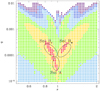 |
Fig. 2 Δχ2 map in the s–q plane. The color coding is set to represent points with <1nσ (red), <2nσ (yellow), <3nσ (green), <4nσ (cyan), <5nσ (blue), and <6nσ (purple), where n = 4. The three encircled regions indicate the positions of the three degenerate local solutions A, Bc, and Bw. |
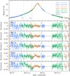 |
Fig. 3 Zoomed-in view of the light curve in the peak region and the residuals from five tested models including 1L1S, 1L2S, and three 2L1S models (solutions A, Bc, and Bw). Although three 2L1S model curves are drawn over the data points in the top panel, it is difficult to distinguish between them withinthe line width due to the severity of the degeneracy among the solutions. |
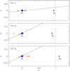 |
Fig. 4 Lens system configurations of the three degenerate 2L1S solutions: A, Bc, and Bw. In each panel, the blue dots, marked by M1 (host) and M2 (planet), are the lens positions, the line with an arrow is the source trajectory, and the cuspy closed curves are the caustics. The dashed circle centered at M1 represents the Einstein ring. The enlarged views in the central magnification regions for the individual solutions are presented inFig. 5. |
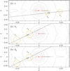 |
Fig. 5 Lens system configurations in the central magnification region for the three 2L1S solutions. Notations are the same as those in Fig. 4. The two orange circles represent the source positions at the times of the major anomalies at t1 and t2 that are marked in Figs. 1 and 3. The size of the circle is scaled to the source size. In the case of solution A, for which the source size cannot be securely measured, the radius of the circle is set to that of the best-fit value. |
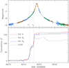 |
Fig. 6 Cumulative distributions of Δχ2 for the three degenerate 2L1S (solutions A, Bc, and Bw) models and 1L2S model with respect to the 1L1S model. The dotted vertical lines denote the times of the major anomalies at t1 and t2 that are marked in Fig. 1. |
5 Angular Einstein radius
In general cases of lensing events, the angular Einstein radius is estimated from a combination of the angular source radius θ* and the normalized source radius ρ by
 (1)
(1)
The value of θ* can be derived from the color and brightness of the source, and the value of ρ is decided from the analysis of the light curve affected by finite-source effects. Then, the prerequisite for the measurement of θE is that a lensing light curve should be affected by finite-source effects to yield the normalized source radius ρ3.
In the case of KMT-2018-BLG-1025, the feasibility of measuring ρ varies depending on the solution. We find that finite-source effects are securely detected according to solutions Bc and Bw; however, according to solution A, the effects are not firmly detected and the model is consistent with a point-source model within 3σ. This is shown in Fig. 7, in which we present the Δχ2 distributions of points in the MCMC chain obtained from the modeling runs of the three degenerate 2L1S solutions. These scatter plots show that the normalized source radii of the B solutions, ρ ~ 7–8 × 10⁻³, are well determined, but only a upper limit, ρmax ~ 5.5 × 10⁻³, can be placed for solution A. As a result, the angular Einstein radius was determined for solutions Bc and Bw, but only a lower limit can be placed for solution A. Below, we describe the procedure of θE estimation for the individual solutions.
The angular source radius and the resulting Einstein radius for each solution was estimated following the routine procedure outlined in Yoo et al. (2004). In the first step of the procedure, we specified the source type by placing the positions of the source and the centroid of the red giant clump (RGC) in the CMD of stars lying in the vicinity of the source. Figure 8 shows the positions of the source, marked by a black cross at (V − I, I) = (2.585 ± 0.029, 21.465 ± 0.003), estimated from solution A, and the RGC centroid, red dot at  , in the instrumental CMD constructed using the pyDIA photometry data of the KMTC I- and V -band images. We note that the source color and brightness estimated from the other solutions, marked by gray crosses and listed in Table 4, result in similar values. The position of the blend, green dot, is also marked. As we show in the following section, the lens is a very low-mass M dwarf, while the color and brightness of the blend correspond to an early main-sequence star or a subgiant. This implies that the contribution of the lens flux to the blended flux is negligible. We calibrated the source color and brightness using the known de-reddened values of the RGC centroid,
  (Bensby et al. 2013; Nataf et al. 2013), as references. From the measured offsets in the color Δ(V − I) and brightness ΔI between the source and RGC centroid, the reddening and extinction corrected values of the source color and brightness were estimated by
 (2)
(2)
The values of  corresponding to the individual solutions are listed in Table 4. The estimated color and brightness are
  , indicating that the source is an early K-type main sequence star. We then converted V − I color into V − K color using the color-color relation of Bessell & Brett (1988), and we estimated the angular source radius using the (V − K) – θ* relation of Kervella et al. (2004). The measured source radii are in the range of 0.67 ≲ θ*∕μas ≲ 0.70. Finally, the angular Einstein radius and the relative lens-source proper motion were estimated by the relations θE = θ*∕ρ and μ = θE∕tE, respectively.
In Table 4, we list the values of θ*, θE, and μ corresponding to the individual solutions. We note that the lower limits of θE and μ are presented for solution A, for which only the upper limit of ρ is constrained. We note that the Einstein radius estimated from solutions B, θE = 0.091 for solution Bc and 0.094 mas Bw, is substantially smaller than ~ 0.5 mas of a typical lensing event produced by an M dwarf with a mass ~0.3 M⊙ located roughly halfway between the lens and source. The angular Einstein radius is related to the lens mass and distance by
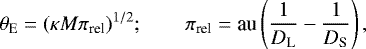 (3)
(3)
where κ = 4G∕(c2au) and DS is the distance to the source. Then, the small value of θE for the solutions B suggests that the lens has a low mass or it is located close to the source.
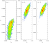 |
Fig. 7 Distributions of points in the MCMC chains for the three degenerate 2L1S solutions. The red, yellow, green, cyan, and blue colors represent points within 1σ, 2σ, 3σ, 4σ, and 5σ, respectively. The significance level was determined so that nσ corresponds to Δχ2 = n2 with rescaled uncertainties. |
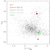 |
Fig. 8 Source (cross mark) position with respect to the centroid of the red giant clump (RGC, red dot) in the instrumental color-magnitude diagram of stars lying in the vicinity of the source. We mark source positions corresponding to the three degenerate solutions, which yield very similar source locations. The position of the blend (green dot) is also marked. |
Source color, brightness, Einstein radius, and proper motion.
6 Physical lens parameters
The lens mass and distance can be unambiguously determined by simultaneously measuring θE and πE, which are related to the physical lens parameters by
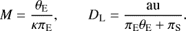 (4)
(4)
Here πS = au∕DS denotes the parallax of the source. In the case of KMT-2018-BLG-1025, only θE was measured for solutions Bc and Bw, and neither θE nor πE was measured for solution A. Although this makes it difficult to uniquely determine M and DL, these parameters can be statistically constrained from a Bayesian analysis with the priors of a lens mass function and a Galactic model.
In the Bayesian analysis, we conducted a Monte Carlo simulation to produce artificial lensing events. For the production of events, we used priors of a mass function to assign lens masses and a Galactic model to assign lens locations and relative lens-source transverse velocities. For the mass function, we used a model constructed by combining the mass functions of Zhang et al. (2019) and Gould (2000), and the model considers not only stellar lenses but also substellar brown dwarfs and stellar remnants. For the physical lens distribution, we used the modified version of the Han & Gould (2003) model, in which the original double-exponential disk model is replaced with the Bennett et al. (2014) model. We note that the distance to the source, DS, is allowed to vary by choosing DS from the physical distribution model of the bulge instead of using a fixed value. For the dynamical distribution of the lens and source motion, we adopted the Han & Gould (1995) model. A detailed description of the adopted priors is given in Han et al. (2020a). The number of events produced by the simulation for each solution is 107. With the events produced by the simulation, posteriors of M and DL were obtained by constructing the probability distributions of events that are consistent with the measured observables. Although the ρ value is not tightly constrained for solution A, we used its distribution obtained based on the MCMC links to weight the posteriors of M and DL.
The posteriors for the host mass, Mh, and distance to the lens are shown in Figs. 9 and 10, respectively. For each posterior, we present three distributions, in which the red and blue distributions are contributions by the bulge and disk lens populations, respectively, and the black distribution is the sum of contributions by both of the lens populations.In Table 5, we list the estimated physical parameters of the host and planet (Mp) masses, distance, and projected physical separation (a⊥) of the planet from its host. For each physical parameter, we chose a median of the probability distribution as a representative value, and the upper and lower limits were estimated as the 16% and 84% ranges of the distributions. The estimated masses of the planet and host are
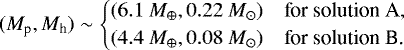 (5)
(5)
The planet mass is in the category of a super-Earth regardless of the solutions, and thus the planet is the eleventh super-Earth planet discovered by microlensing. The host mass varies depending on the solutions: a mid-M dwarf for solution A and a very late M dwarf or possibly a substellar brown dwarf for solutions B. The estimated distance to the lens is
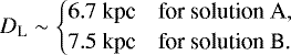 (6)
(6)
The host mass estimated from the solutions B is substantially smaller than the corresponding value of solution A. This is because the host mass of solution A is estimated mostly based on the single constraint of the event timescale, tE ~ 9.6 days, but the mass of solutions B is estimated with the additional constraint of the small Einstein radius, θE ~ 0.09 mas. For the same reason, the distance to the lens predicted by solutions B, ~ 7.5 kpc, is greater than the distance expected from solution A, ~6.7 kpc.
The degeneracy between solutions A and B can very likely be lifted if the lens and source can be resolved from future follow-up observations using a high-resolution adaptive optics (AO) instrument. KMT-2018-BLG-1025 presents an unusual case for which the degeneracy can be lifted purely by the proper motion measurement, which is the most robust result from AO follow-up observations. From Fig. 7, ρSol A < 5.5 × 10⁻³ and ρSol B > 5.9 × 10⁻³, both at 3 σ, while from Tables 3 and 4, the quantity θ* ∕tE is about 10% larger for solution A than solutions Bc and Bw. Therefore, the 3σ limits for μ = θ*∕(ρtE) barely overlap. Most likely, the actual proper motion measurement will be well away from this boundary, for example, near the best fits μ ≃3.8 mas yr−1 (for solutions B) or μ ≃ 5.7 mas yr−1 (for solutionA). Only if the measured value is about halfway between the boundary will the correct solution remain undetermined. We note that the long tail in the solution A distribution, which prevented a precise estimate of θE and μ for this case, does not affect the resolution of the degeneracy: if the true value of ρ is in this tail, then the proper motion will be high, and solution A will be unambiguously favored. To be confident of detecting the lens, one should allow for proper motions as low as μ ~ 3 mas yr−1, which are permitted by solutions B. However, even at this slow pace, the source and lens will be separated by 30 mas in 2028, theearliest possible date for the first AO light 30m class telescopes. At that point, the source and lens can be easily resolved. By contrast, the close–wide degeneracy between solutions Bc and Bw cannot be resolved because the relative proper motions expected from the degenerate solutions are similar to one another.
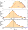 |
Fig. 9 Bayesian posteriors of the host mass for the three degenerate 2L1S solutions. The three curves in each panel represent contributions by the disk (blue), bulge (red), and total (black) lens populations. The solid vertical line represents the median, and the two dotted vertical lines indicate the 1σ range of the distribution. |
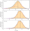 |
Fig. 10 Bayesian posteriors of the lens distance for the three 2L1S solutions. Notations are the same as those in Fig. 9. |
Physical lens parameters.
7 Conclusion
We have reported the discovery of a super-Earth planet that was found from the analysis of the lensing event KMT-2018-BLG-1025. The planetary signal in the lensing light curve had not been noticed during the season of the event discovery, and it was found from the systematic inspection of high-magnification events in the KMTNet data collected in and before the 2018 season. We identified three degenerate solutions, in which the ambiguity between a pair of solutions was caused by the previously known close–wide degeneracy, and the degeneracy between these and the other solution was a new type that had not been reported before. The estimated mass ratio between the planet and host was q ~ 0.8 × 10⁻⁴ for one solution and ~1.6 × 10⁻⁴ for the other pair of solutions. From the Bayesian analysis carried out with the measured observables, we estimated that the masses of the planet and host and the distance to the lens were (Mp, Mh, DL) ~ (6.1 M⊕, 0.22 M⊙, 6.7 kpc) for one solution and ~(4.4 M⊕, 0.08 M⊙, 7.5 kpc) for the other solutions. The planet mass was in the category of a super-Earth regardless of the solutions, making the planet the eleventh super-Earth planet discovered by microlensing. Due to the substantial difference between the relative lens-source proper motions expected from the two sets of solutions, the degeneracy between the solutions can be lifted by resolving the lens and source from future high resolution imaging observations. These observations will also yield the mass and distance of the lens, and thus the mass of the planet.
Acknowledgements
Work by C.H. was supported by the grants of National Research Foundation of Korea (2020R1A4A2002885 and 2019R1A2C2085965). Work by A.G. was supported by JPL grant 1500811. This research has made use of the KMTNet system operated by the Korea Astronomy and Space Science Institute (KASI) and the data were obtained at three host sites of CTIO in Chile, SAAO in South Africa, and SSO in Australia. The OGLE project has received funding from the National Science Centre, Poland, grant MAESTRO 2014/14/A/ST9/00121 to AU.
References
- Alard, C., & Lupton, R. H. 1998, ApJ, 503, 325 [NASA ADS] [CrossRef] [Google Scholar]
- Albrow, M. 2017, MichaelDAlbrow/pyDIA: Initial Release on Github, Version v1.0.0, Zenodo, https://doi.org/10.5281/zenodo.268049 [Google Scholar]
- Albrow, M., Horne, K., Bramich, D. M., et al. 2009, MNRAS, 397, 2099 [NASA ADS] [CrossRef] [Google Scholar]
- Alcock, C., Allsman, R. A., Alves, D., et al. 1997, ApJ, 479, 119 [NASA ADS] [CrossRef] [Google Scholar]
- An, J. H. 2005, MNRAS, 356, 1409 [NASA ADS] [CrossRef] [Google Scholar]
- Batista, V., Beaulieu, J.-P., Bennett, D. P., et al. 2015, ApJ, 808, 170 [NASA ADS] [CrossRef] [Google Scholar]
- Beaulieu, J.-P., Bennett, D. P., Fouqué, P., et al. 2006, Nature, 439, 437 [NASA ADS] [CrossRef] [PubMed] [Google Scholar]
- Bennett, D. P., Bond, I. A., Udalski, A., et al. 2008, ApJ, 684, 663 [NASA ADS] [CrossRef] [Google Scholar]
- Bennett, D. P., Batista, V., Bond, I. A., et al. 2014, ApJ, 785, 155 [NASA ADS] [CrossRef] [Google Scholar]
- Bennett, D. P., Bhattacharya, A., Anderson, J., et al. 2015, ApJ, 808, 169 [NASA ADS] [CrossRef] [Google Scholar]
- Bennett, D. P., Bhattacharya, A., Beaulieu, J.-P., et al. 2020, AJ, 159, 68 [Google Scholar]
- Bensby, T., Yee, J. C., Feltzing, S., et al. 2013, A&A, 549, A147 [NASA ADS] [CrossRef] [EDP Sciences] [Google Scholar]
- Bessell, M. S.,& Brett, J. M. 1988, PASP, 100, 1134 [NASA ADS] [CrossRef] [Google Scholar]
- Bhattacharya, A., Beaulieu, J.-P., Bennett, D. P., et al. 2018, AJ, 156, 289 [Google Scholar]
- Bhattacharya, A., Bennett, D. P.. Beaulieu, J.-P., et al. 2020, AJ, submitted [arXiv:2009.02329] [Google Scholar]
- Bond, I. A., Abe, F., Dodd, R. J., et al. 2001, MNRAS, 327, 868 [Google Scholar]
- Bond, I. A., Bennett, D. P., Sumi, T., et al. 2017, MNRAS, 469.2434 [Google Scholar]
- Choi, J.-Y., Shin, I.-G., Han, C., et al. 2012, ApJ, 756, 48 [NASA ADS] [CrossRef] [Google Scholar]
- Chung, S.-J., Han, C., Park, B.-G., et al. 2005, ApJ, 630, 535 [NASA ADS] [CrossRef] [Google Scholar]
- Dominik, M. 1999, A&A, 349, 108 [NASA ADS] [Google Scholar]
- Gaudi, B. S. 2012, ARA&A, 50, 411 [NASA ADS] [CrossRef] [Google Scholar]
- Gaudi, B. S, & Gould, A. 1997, ApJ, 486, 85 [NASA ADS] [CrossRef] [Google Scholar]
- Gould, A. 1992, ApJ, 392, 442 [NASA ADS] [CrossRef] [EDP Sciences] [Google Scholar]
- Gould, A. 2000, ApJ, 535, 928 [NASA ADS] [CrossRef] [Google Scholar]
- Gould, A., & Loeb, A. 1992, ApJ, 396, 104 [NASA ADS] [CrossRef] [Google Scholar]
- Gould, A., Udalski, A., An, D., et al. 2006, ApJ, 644, L37 [NASA ADS] [CrossRef] [Google Scholar]
- Gould, A., Udalski, A., Shin, I.-G., et al. 2014, Science, 345, 46 [NASA ADS] [CrossRef] [Google Scholar]
- Gould, A., Ryu, Y.-H., Calchi Novati, S., et al. 2020, J. Korean Astron. Soc., 53, 9 [Google Scholar]
- Griest, K., & Safizadeh, N. 1998, ApJ, 500, 37 [NASA ADS] [CrossRef] [Google Scholar]
- Griest, K., Alcock, C., Axelrod, T. S., et al. 1991, ApJ, 372, L79 [NASA ADS] [CrossRef] [Google Scholar]
- Han, C. 2006, ApJ, 638, 1080 [NASA ADS] [CrossRef] [Google Scholar]
- Han, C. 2009a, ApJ, 691, L9 [NASA ADS] [CrossRef] [Google Scholar]
- Han, C. 2009b, ApJ, 691, 452 [NASA ADS] [CrossRef] [Google Scholar]
- Han, C., & Gould, A. 1995, ApJ, 447, 53 [NASA ADS] [CrossRef] [Google Scholar]
- Han, C., & Gould, A. 2003, ApJ, 592, 172 [NASA ADS] [CrossRef] [Google Scholar]
- Han, C., Bond, I. A., Gould, A., et al. 2018, AJ, 156, 226 [Google Scholar]
- Han, C., Shin, I.-G., Jung, Y. K., et al. 2020a, A&A, 641, A105 [CrossRef] [EDP Sciences] [Google Scholar]
- Han, C., Udalski, A., Kim, D., et al. 2020b, A&A, 642, A110 [EDP Sciences] [Google Scholar]
- Herrera-Martín, A., Albrow, M. D., Udalski, A., et al. 2020, AJ, 159, 256 [Google Scholar]
- Hwang, K.-H., Choi, J.-Y., Bond, I. A., et al. 2013, AJ, 778, 55 [Google Scholar]
- Hwang, K.-H., Kim, H.-W., Kim, D.-J., et al. 2018, J. Korean Astron. Soc., 51, 197 [Google Scholar]
- Jung, Y. K., Udalski, A., Zang, W., et al. 2020, AJ, 160, 255 [Google Scholar]
- Kervella, P., Thévenin, F., Di Folco, E., & Ségransan, D. 2004, A&A, 426, 29 [Google Scholar]
- Kim, S.-L., Lee, C.-U., Park, B.-G., et al. 2016, J. Korean Astron. Soc., 49, 37 [Google Scholar]
- Kim, D.-J., Kim, H.-W., Hwang, K.-H., et al. 2018, AJ, 155, 76 [NASA ADS] [CrossRef] [Google Scholar]
- Mao, S., & Paczyński, B. 1991, ApJ, 374, L37 [Google Scholar]
- Mróz, P., Udalski, A., Skowron, J., et al. 2019, ApJS, 244, 29 [Google Scholar]
- Mróz, P., Poleski, R., Gould, A., et al. 2020, ApJ, 903, L11 [Google Scholar]
- Nataf, D. M., Gould, A., Fouqué, P., et al. 2013, ApJ, 769, 88 [NASA ADS] [CrossRef] [Google Scholar]
- Paczyński, B. 1991, ApJ, 371, L63 [NASA ADS] [CrossRef] [Google Scholar]
- Park, H., Han, C., Gould, A., et al. 2014, ApJ, 787, 71 [Google Scholar]
- Ryu, Y.-H., Udalski, A., Yee, J. C., et al. 2020, AJ, 160, 183 [Google Scholar]
- Shvartzvald, Y., Yee, J. C., Calchi Novati, S., et al. 2017, ApJ, 840, L3 [NASA ADS] [CrossRef] [Google Scholar]
- Skowron, J., Ryu, Y.-H., Hwang, K.-H., et al. 2018, Acta Astron., 68, 43 [Google Scholar]
- Sumi, T., & Penny, M. T. 2016, ApJ, 827, 139 [NASA ADS] [CrossRef] [Google Scholar]
- Tomaney, A. B., & Crotts, A. P. S. 1996, AJ, 112, 2872 [NASA ADS] [CrossRef] [Google Scholar]
- Udalski, A. 2003, Acta Astron., 53, 291 [NASA ADS] [Google Scholar]
- Udalski, A., Szymański, M., Kałużny, J., et al. 1994, Acta Astron. 44, 1 [Google Scholar]
- Udalski, A., Szymański, M. K., & Szymański, G. 2015, Acta Astron., 65, 1 [NASA ADS] [Google Scholar]
- Udalski, A., Ryu, Y.-H., Sajadian, S., et al. 2018, Acta Astron., 68, 1 [Google Scholar]
- Valencia, D., Sasselov, D. D., & O’Connell, R. J. 2007, ApJ, 656, 545 [Google Scholar]
- Vandorou, A., Bennett, D. P.. Beaulieu, J.-P., et al. 2020, AJ, 160, 121 [Google Scholar]
- Yee, J. C., Shvartzvald, Y., Gal-Yam, A., et al. 2012, ApJ, 755, 102 [NASA ADS] [CrossRef] [Google Scholar]
- Yoo, J., DePoy, D. L., Gal-Yam, A., et al. 2004, ApJ, 603, 139 [Google Scholar]
- Zhang, X., Zang, W., Udalski, A., et al. 2020, AJ, 159, 116 [CrossRef] [Google Scholar]
- Zhu, W., Penny, M., Mao, S., Gould, A., & Gendron, R. 2014, ApJ, 788, 73 [NASA ADS] [CrossRef] [Google Scholar]
We note that the term “super-Earth” refers only to the mass of the planet, and so it does not imply anything about the atmosphere structure, surface conditions, or size of the planet.
The data are available at http://astroph.chungbuk.ac.kr/~cheongho/data.html
The angular Einstein radius can also be measured by separately imaging the lens and source. By resolving the images, one can measure the vector separation Δθ between the lens and source and hence their heliocentric relative proper motion by μhel = Δθ∕Δt, where Δt represents the time elapsed since the event. Then, the Einstein radius is determined by θE = μgeotE. Here the geocentric relative proper motion is related to μhel by μgeo = μhel −v⊕,⊥πrel∕au, where v⊕,⊥ is Earth’s velocity projected on the plane of the sky at t0. Due to the long time span Δt required for the lens–source resolution together with the limited access to high-resolution instrument, there exist just five cases of planetary lens events for which the values of θE are measured by this method: OGLE-2005-BLG-071 (Bennett et al. 2020), OGLE-2005-BLG-169 (Batista et al. 2015; Bennett et al. 2015), OGLE-2012-BLG-0950 (Bhattacharya et al. 2018), MOA 2013 BLG-220 (Vandorou et al. 2020), and MOA-2007-BLG-400 (Bhattacharya et al. 2020).
All Tables
All Figures
|
Fig. 1 Light curve of KMT-2018-BLG-1025. Upper and lower panels: whole view and the zoomed-in view of the peak region, respectively. The colors of data points indicate the observatories, as given in the legend. The curve plotted over the data points is the 1L1S model, for which the residuals in the peak region are presented in the bottom panel. The dotted vertical lines at t1 ~ 8274.38 and t2 ~8274.66 indicate the respective times of the bump and dip in the residuals to the 1L1S model. |
| In the text | |
|
Fig. 2 Δχ2 map in the s–q plane. The color coding is set to represent points with <1nσ (red), <2nσ (yellow), <3nσ (green), <4nσ (cyan), <5nσ (blue), and <6nσ (purple), where n = 4. The three encircled regions indicate the positions of the three degenerate local solutions A, Bc, and Bw. |
| In the text | |
|
Fig. 3 Zoomed-in view of the light curve in the peak region and the residuals from five tested models including 1L1S, 1L2S, and three 2L1S models (solutions A, Bc, and Bw). Although three 2L1S model curves are drawn over the data points in the top panel, it is difficult to distinguish between them withinthe line width due to the severity of the degeneracy among the solutions. |
| In the text | |
|
Fig. 4 Lens system configurations of the three degenerate 2L1S solutions: A, Bc, and Bw. In each panel, the blue dots, marked by M1 (host) and M2 (planet), are the lens positions, the line with an arrow is the source trajectory, and the cuspy closed curves are the caustics. The dashed circle centered at M1 represents the Einstein ring. The enlarged views in the central magnification regions for the individual solutions are presented inFig. 5. |
| In the text | |
|
Fig. 5 Lens system configurations in the central magnification region for the three 2L1S solutions. Notations are the same as those in Fig. 4. The two orange circles represent the source positions at the times of the major anomalies at t1 and t2 that are marked in Figs. 1 and 3. The size of the circle is scaled to the source size. In the case of solution A, for which the source size cannot be securely measured, the radius of the circle is set to that of the best-fit value. |
| In the text | |
|
Fig. 6 Cumulative distributions of Δχ2 for the three degenerate 2L1S (solutions A, Bc, and Bw) models and 1L2S model with respect to the 1L1S model. The dotted vertical lines denote the times of the major anomalies at t1 and t2 that are marked in Fig. 1. |
| In the text | |
|
Fig. 7 Distributions of points in the MCMC chains for the three degenerate 2L1S solutions. The red, yellow, green, cyan, and blue colors represent points within 1σ, 2σ, 3σ, 4σ, and 5σ, respectively. The significance level was determined so that nσ corresponds to Δχ2 = n2 with rescaled uncertainties. |
| In the text | |
|
Fig. 8 Source (cross mark) position with respect to the centroid of the red giant clump (RGC, red dot) in the instrumental color-magnitude diagram of stars lying in the vicinity of the source. We mark source positions corresponding to the three degenerate solutions, which yield very similar source locations. The position of the blend (green dot) is also marked. |
| In the text | |
|
Fig. 9 Bayesian posteriors of the host mass for the three degenerate 2L1S solutions. The three curves in each panel represent contributions by the disk (blue), bulge (red), and total (black) lens populations. The solid vertical line represents the median, and the two dotted vertical lines indicate the 1σ range of the distribution. |
| In the text | |
|
Fig. 10 Bayesian posteriors of the lens distance for the three 2L1S solutions. Notations are the same as those in Fig. 9. |
| In the text | |
Current usage metrics show cumulative count of Article Views (full-text article views including HTML views, PDF and ePub downloads, according to the available data) and Abstracts Views on Vision4Press platform.
Data correspond to usage on the plateform after 2015. The current usage metrics is available 48-96 hours after online publication and is updated daily on week days.
Initial download of the metrics may take a while.