| Issue |
A&A
Volume 649, May 2021
|
|
|---|---|---|
| Article Number | A29 | |
| Number of page(s) | 13 | |
| Section | Planets and planetary systems | |
| DOI | https://doi.org/10.1051/0004-6361/202039247 | |
| Published online | 07 May 2021 | |
The GAPS programme at TNG
XXX. Atmospheric Rossiter-McLaughlin effect and atmospheric dynamics of KELT-20b★
1
INAF – Osservatorio Astrofisico di Arcetri,
Largo Enrico Fermi 5,
50125
Firenze,
Italy
e-mail: This email address is being protected from spambots. You need JavaScript enabled to view it.
2
INAF – Osservatorio Astronomico di Brera,
Via E. Bianchi, 46,
23807
Merate (LC), Italy
3
Anton Pannekoek Institute for Astronomy, University of Amsterdam Science Park 904 1098 XH
Amsterdam,
The Netherlands
4
Università degli Studi di Milano Bicocca,
Piazza dell’Ateneo Nuovo, 1,
20126
Milano, Italy
5
Department of Physics, University of Warwick,
Coventry
CV4 7AL, UK
6
INAF – Osservatorio Astrofisico di Torino,
Via Osservatorio 20,
10025
Pino Torinese (TO),
Italy
7
Centre for Exoplanets and Habitability, University of Warwick,
Gibbet Hill Road,
Coventry
CV4 7AL, UK
8
INAF – Osservatorio Astronomico di Roma,
Via Frascati 33,
00078
Monte Porzio Catone (Roma),
Italy
9
Astronomy Department and Van Vleck Observatory, Wesleyan University,
Middletown,
CT
06459, USA
10
INAF – Osservatorio Astronomico di Padova,
Vicolo dell’Osservatorio, 5,
35122
Padova (PD), Italy
11
INAF – Osservatorio Astrofisico di Catania,
Via S. Sofia 78,
95123
Catania,
Italy
12
INAF – Osservatorio Astronomico di Palermo,
Piazza del Parlamento, 1,
90134
Palermo, Italy
13
Department of Physics, University of Rome “Tor Vergata”,
Via della Ricerca Scientifica 1,
00133
Rome, Italy
14
Max Planck Institute for Astronomy,
Königstuhl 17,
69117,
Heidelberg, Germany
15
Department of Astronomy, University of Geneva,
Chemin des Maillettes 51,
1290
Versoix, Suisse
16
INAF – Osservatorio Astronomico di Capodimonte,
Salita Moiariello 16,
80131
Napoli,
Italy
17
INAF – Fundación Galileo Galilei,
Rambla José Ana Fernandez Pérez 7,
38712
Breña Baja (TF),
Spain
18
INAF – Osservatorio Astronomico di Cagliari,
Via della Scienza 5,
09047
Cuccuru Angius,
Selargius (CA), Italy
19
INAF – Osservatorio Astronomico di Trieste,
Via Giambattista Tiepolo, 11,
34131
Trieste, Italy
20
Aix-Marseille Université, CNRS, CNES, LAM,
Marseille,
France
21
Dipartimento di Fisica e Astronomia Galileo Galilei – Università di Padova,
Vicolo dell’Osservatorio 2,
35122
Padova, Italy
Received:
24
August
2020
Accepted:
16
March
2021
Abstract
Context. Transiting ultra-hot Jupiters are ideal candidates for studying the exoplanet atmospheres and their dynamics, particularly by means of high-resolution spectra with high signal-to-noise ratios. One such object is KELT-20b. It orbits the fast-rotating A2-type star KELT-20. Many atomic species have been found in its atmosphere, with blueshifted signals that indicate a day- to night-side wind.
Aims. We observe the atmospheric Rossiter-McLaughlin effect in the ultra-hot Jupiter KELT-20b and study any variation of the atmospheric signal during the transit. For this purpose, we analysed five nights of HARPS-N spectra covering five transits of KELT-20b.
Methods. We computed the mean line profiles of the spectra with a least-squares deconvolution using a stellar mask obtained from the Vienna Atomic Line Database (Teff = 10 000 K, log g = 4.3), and then we extracted the stellar radial velocities by fitting them with a rotational broadening profile in order to obtain the radial velocity time-series. We used the mean line profile residuals tomography to analyse the planetary atmospheric signal and its variations. We also used the cross-correlation method to study a previously reported double-peak feature in the FeI planetary signal.
Results. We observed both the classical and the atmospheric Rossiter-McLaughlin effect in the radial velocity time-series. The latter gave us an estimate of the radius of the planetary atmosphere that correlates with the stellar mask used in our work (Rp+atmo∕Rp = 1.13 ± 0.02). We isolated the planetary atmospheric trace in the tomography, and we found radial velocity variations of the planetary atmospheric signal during transit with an overall blueshift of ≈10 km s−1, along with small variations in the signal depth, and less significant, in the full width at half maximum (FWHM). We also find a possible variation in the structure and position of the FeI signal in different transits.
Conclusions. We confirm the previously detected blueshift of the atmospheric signal during the transit. The FWHM variations of the atmospheric signal, if confirmed, may be caused by more turbulent condition at the beginning of the transit, by a variable contribution of the elements present in the stellar mask to the overall planetary atmospheric signal, or by iron condensation. The FeI signal show indications of variability from one transit to the next.
Key words: planetary systems / techniques: spectroscopic / techniques: radial velocities / planets and satellites: atmospheres / stars: individual: KELT-20
Based on observations made with the Italian Telescopio Nazionale Galileo (TNG) operated by the Fundación Galileo Galilei (FGG) of the Istituto Nazionale di Astrofisica (INAF) at the Observatorio del Roque de los Muchachos (La Palma, Canary Islands, Spain).
© ESO 2021
1 Introduction
A very interesting category of exoplanets is represented by the transiting ultra-hot Jupiters (UHJs; Bell & Cowan 2018), which are highly irradiated Jupiter-size planets with day-side temperatures higher than 2200 K (Parmentier et al. 2018). Transiting UHJs are ideal laboratories for studying planetary atmospheres. Their inflated atmospheres and high equilibrium temperatures (Teq) result in strong signals and striking peculiar conditions for a planetary body. Their atmospheres are rich in atomic and molecular species. For example, CrII, FeI, FeII, MgII, NaI, ScII, TiII, and YII have been detected in KELT-9b, the hottest UHJ known so far (Teq = 4050 K), with additional evidence of the presence of CaI, CrI, CoI, and SrII (Hoeijmakers et al. 2018, 2019). Because neutral and ionised iron are present in their atmospheres, UHJs can be used to study the atmospheric Rossiter-McLaughlin effect (Borsa et al. 2019). The signal coming from their atmosphere correlates with the stellar mask that is used to compute the mean line profile of the spectra and to recover the stellar radial velocity (RV), resulting in an additional absorption in the mean line profile that causes an apparent RV variation similar to the classical Rossiter-McLaughlin effect (RML). In addition to this, UHJs usually have very different atmospheric conditions (e.g. in temperature and chemical composition) at their day and night side that may result in day- to night-side wind (Ehrenreich et al. 2020; Heng & Showman 2015). High-resolution spectroscopy may be used to study the RV variations of the atmospheric signal in order to search for the presence of winds or any other type of atmospheric turbulence.
KELT-20b (Lund et al. 2017), also known as MASCARA-2b (Talens et al. 2018), is a well-known ultra-hot Jupiter orbiting a fast-rotatingA-type star. With a period of 3.47 days and a semi-major axis of 0.0542 au, KELT-20b is highly irradiated by its host star (A2, Teff = 8980 K, mV = 7.6), and its atmosphere reaches Teq = 2260 K (see Table 1 for more details of the system).
Many atomic species such as FeI, FeII, CaII, NaI, and HI have been detected in its atmosphere through transit spectroscopy, while there are only tentative detections of MgI and CrII (Casasayas-Barris et al. 2018, 2019; Hoeijmakers et al. 2020; Nugroho et al. 2020; Stangret et al. 2020). There are also indications of a day- to night-side wind by a blueshift of − 6.3 ± 0.8 km s−1 in the FeI signal and − 2.8 ± 0.8 km s−1 in that due to FeII (Stangret et al. 2020; Hoeijmakers et al. 2020; Nugroho et al. 2020).
We observed KELT-20 in the framework of the Global Architecture of Planetary Systems (GAPS) project, which is an Italian project dedicated to the search and characterisation of exoplanets (PI: G. Micela; Covino et al. 2013). One of the GAPS main lines of research in particular focuses on the study of exoplanet atmospheres using transmission and emission spectroscopy (Borsa et al. 2019; Pino et al. 2020; Guilluy et al. 2020). Using our data and public data of KELT-20 taken with the same instrument (HARPS-N), we studied the classical (Rossiter 1924; McLaughlin 1924) and atmospheric RML effects of KELT-20b from the RV time-series, along with the variations in atmospheric trace during the planetary transits from the mean line profile tomography.
The dataset used in this work is described in Sect. 2, and the method we used to obtain the stellar mean line profiles and the RV time-series is detailed in Sect. 3. The classical and atmospheric RML effectsare shown in Sect. 4. The variations in atmospheric trace during the transit and the methods we used to detect them from the mean line profile tomography are described in Sect. 5. In Sect. 6 we describe the cross-correlation with a FeI model performed in order to compare our results with those found in the literature. Finally, our conclusions are presented in Sect. 7.
Physical and orbital parameters of the KELT-20 system (also known as MASCARA-2 or HD 185603).
Data summary.
2 Data sample
We analysed five transits of KELT-20b observed with the high-resolution echelle spectrograph HARPS-N (Cosentino et al. 2012) installed at the Telescopio Nazionale Galileo (TNG) at the Roque de los Muchachos Observatory (La Palma, Spain). HARPS-N is an optical spectrograph with a resolving power R = 115 000 and wavelength coverage 383–693 nm. It is a twin of the HARPS spectrograph that is installed at the 3.6 m telescope of the ESO-LaSilla Observatory, down to the Data Reduction Software (DRS) optimised for exoplanet search.
We observed two transits (2019 August 26 and 2019 September 02) in the framework of the GAPS programme, while the other three transits are public data retrieved from the HARPS-N archive (2017 August 16: PID CAT17A_38 PI: Rebolo; 2018 July 12, and 2018 July 19: PID CAT18A_34, PI Casasayas-Barris). The GAPS observations were taken in the GIARPS mode (Claudi et al. 2016), which allows the simultaneous use of the HARPS-N and GIANO-B (Oliva et al. 2012; Origlia et al. 2014) spectrographs. GIANO-B is a high-resolution (R = 50 000) near-infrared echelle spectrograph covering the wavelength range from 950 to 2450 nm. For this work, we used only the HARPS-N data.
A summary of the acquired HARPS-N spectra in the five transit nights is shown in Table 2. We rejected 14 spectra taken during night 2 because of their low signal-to-noise ratio (S/N). All five transits are complete, and out-of-transit spectra were taken before and after the transit in each night.
We worked on spectra reduced with the HARPS-N DRS (Cosentino et al. 2014). The barycentric correction was therefore already applied.
3 Mean line profiles
While the HARPS-N DRS is a very powerful tool, it is not optimised for hot stars such as KELT-20. The resulting cross-correlation functions (CCFs) are obtained by using a stellar mask designed to work with a G2-type star, which is the hottest stellar maskavailable in the DRS mask library.
We decided therefor to compute the mean line profile using the least-squares deconvolution software (LSD, Donati et al. 1997) with a stellar mask obtained from the VALD3 database1 (Piskunov et al. 1995; Ryabchikova et al. 2015). We downloaded stellar masks for Teff = 9000 K and Teff = 10 000 K, both with log g = 4.31, solar metallicity, micro-turbulence ν = 2 km s−1, and wavelength range 3900–7000 Å. While our results using both masks agree well, we show here only those obtained with Teff = 10 000 K, in which the stellar and planetary signals are stronger (see Fig. 1, where the Teff = 10 000 K profile is almost twice as deep as the Teff = 9000 K one). This may indicate a higher Teff for KELT-20 than previously found.
To apply the LSD, we first normalised all our spectra using a self-developed automated procedure (Rainer et al. 2016). In order to avoid most of the telluric line contamination and the heavy contribution of the stellar Balmer lines (extremely strong, as expected forthe KELT-20 spectral type, and with a different shape), we then cut them, and we kept only the wavelength ranges 4415–4805, 4915–5870, 6050–6265, and 6335–6450 Å. We ran the LSD software on each individual spectrum to obtain the mean line profiles.
We fitted all the mean line profiles with a rotational broadening function (see Fig. 1) using the formula in Eq. (1) (Gray 2008),
![Mathematical equation: \begin{equation*} f(x) = 1-a \frac{2(1-u) \sqrt{1-\left( \frac{x-x_0}{x_l}\right) ^{2}} + 0.5\pi u \left[1- \left(\frac{x-x_0}{x_l}\right)^{2}\right]} {{\pi}x_l \left(1-\frac{u}{3} \right)},\end{equation*}](/articles/aa/full_html/2021/05/aa39247-20/aa39247-20-eq2.png) (1)
(1)
where a is the depth of the profile, x0 is the centre (i.e. the RV value), xl is the vsini⋆ of the star, and u is the linear limb-darkening (LD) coefficient (listed in Table 1). We thus recovered both the RVs and the projected rotational velocities (v sini⋆) for all observed spectra. We found v sin i⋆ = 116.7 ± 0.7 km s−1 by averaging the vsini⋆ of all the out-of-transit spectra. We did not use the in-transit spectra in order to avoid the Doppler shadow affecting our result.
We also computed the vsini⋆ using the Fourier transform method (Smith & Gray 1976; Dravins et al. 1990). Because of the fast rotation of KELT-20, we were able to use the first three zero positions of the Fourier transform of all our mean line profiles to derive the projected rotational velocity. Using only the out-of-transit spectra, we found an average value of v sini⋆ = 116.23 ± 1.25 km s−1, which aligns well with that obtained by the profile fitting. We note here that in case of a fast-rotating star like this, this method is independent of other broadening effects such as macro-turbulence, and it only depends on the LD coefficient. We therefore report this value in Table 1, although the error is larger than that obtained with the profile fitting. The average value of the ratio of the first two zero-positions results in q2 ∕q1 = 1.805 ± 0.036, which is compatible with a rigid rotation (1.72 < q2∕q1 < 1.83, Reiners & Schmitt (2002)).
We computed the stellar rotational period as p⋆ = 2πR⋆∕veq, using R⋆, v sini⋆, and inclination i from Table 1. We considered the orbit inclination i equal to the stellar inclination i⋆ because the projected obliquity λ is compatible with a zero value. We found a stellar rotational period of 0.695 ± 0.027 days, which is almost exactly one fifth of the planetary period. This may suggest a resonance between the stellar and planetary rotation.
We performed a linear fit on all the out-of-transit RVs to recover the systemic velocity, and we found VSys = −24.48 ± 0.04 km s−1. This value is slightly lower than the values found in the literature (see Table 1), but the determination of the systemic velocity may vary depending on the instrument and method used to estimate it. We also computed VSys independently for the five nights, and we noted a weak but significant downward trend that may be worth keeping in mind in further studies (see Fig. 2).
In Fig. 3 we show the RVs corrected for the different VSys (so that the five nights align on the average VSys value) phase-folded using the known orbital value of KELT-20b (P = 3.474119 days, see Table 1). The RML effect is clearly visible.
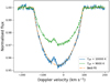 |
Fig. 1 Mean line profile of a single KELT-20 spectrum obtained with the LSD software and Teff = 10 000 K (solid blue line) along with the rotational broadening fit (dash-dotted orange line). For comparison, the mean line profile of the same spectrum with the Teff = 9000 K is shown (dashed green line). The Doppler shadow of the planet is clearly visible as a bump in both lines. |
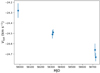 |
Fig. 2 Systemic velocity of the five nights: a weak downward trend is clearly visible. |
4 Classical and atmospheric RML effects
The RML effect is visible in all observation nights (see Fig. 3). We averaged the phase-folded RV data of all transits using a 0.002 phase bin, and we compared them with a theoretical model obtained using the already known system parameters of Table 1, using our value for the systemic velocity. The RML model was computed with the Rmcl model class of the PyAstronomy2 package (Czesla et al. 2019) of Python3 (Van Rossum & Drake Jr 1995), which implements the analytical model RV curves for the RML effect given by Ohta et al. (2005).
The comparison of the data and the theoretical model is shown in Fig. 4. The model appears to overestimate the amplitude of the RML effect, but we know from a previous study of KELT-9b (Borsa et al. 2019) that the atmospheric RML effect may combine with the classical RML effect and that the resulting RVs carry both signals.
The atmospheric RML effect is similar to the classical effect: an apparent stellar RV variation due to the deformation of the stellar lines. While in the classical RML effect the deformation is caused by the occultation of part of the stellar disk by the transiting planet, in the atmospheric RML effect, we have an additional absorption signal because the planetary atmosphericspectrum correlates with the mask that is used to compute the CCF or the LSD mean line profile. This occurs only in the case of extremely hot planetary atmospheres that show a chemical composition similar to that of late-type stars (in particular due to the presence of neutral or ionised iron), and their atmospheric spectrum therefore correlates with the same mask as is used for the host stars (e.g. in this case, the stellar mask contains most of the elements found in the atmosphere of KELT-20b, with more than half of the lines being either FeI or FeII).
In the tomography of the line profile residuals (Fig. 5, see Sect. 5 for details), not only the Doppler shadow is visible (red hues), but also the planetary atmospheric trace (blue hues). The latter shifts by the change in planetary orbital RV during transit, confirming that the planetary atmospheric spectrum correlates with the stellar mask, and thus it shows up in the line residuals as an additional absorption line situated at the planet RV. The Doppler shadow and the atmospheric trace are aligned in such a way that the atmospherictrace is expected to affect the RVs derived from the mean line profiles in the opposite way as the Doppler shadow, so that the net result would be a smaller amplitude of the RML effect, as is seen in Fig. 4.
We then subtracted the RML theoretical model from our data. The resulting RV residuals show the atmosphericRML effect. It goes in the opposite direction from the classical RML effect because it modifies the line profile as an additional absorption instead of a bump. We fit the RV residuals (see Fig. 6) using the Rmcl fit class of the same PyAstronomy package as before. We interpret the resulting value Rp ∕R⋆ = 0.060 ± 0.002 given by the fit as Ratmo∕R⋆, where Ratmo represents the extension of the atmosphere that correlates with the stellar mask we used if the atmosphere were shaped like a disk. The error on this value was estimated using the pymc4 package of Python. When we compare this result with the planetary radius Rp ∕R⋆ = 0.115 ± 0.002, the atmospheric area is ~27% of the whole planetary photometric area. If we hypothesise the simplest scenario of a spherical atmosphere, we can then derive Rp+atmo = 1.13 ± 0.02 Rp, only for theportion of the planetary atmosphere whose spectrum correlates with the stellar mask. This value agrees well with the results from Casasayas-Barris et al. (2019), who found Rp+atmo = 1.11 ± 0.03 Rp for FeII. The slightly higher value found here may be due to the presence of a few lines of other elements, such as CaII, for which Casasayas-Barris et al. (2019) found Rp+atmo = 1.19 ± 0.03 Rp.
We note here that adjusting the classical RML theoretical model by varying the system parameters values inside their error ranges alters our atmospheric RML result only slightly. It remains in agreement with the Ratmo∕R⋆ = 0.060 ± 0.002 value within the 1σ uncertainty.
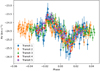 |
Fig. 3 RV data phase-folded using the known orbital period of KELT-20b (P = 3.474119 days). The RV values were shifted by the difference between the individual VSys of each night and the average VSys value to account for the trend found in our data. |
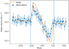 |
Fig. 4 Comparison of the observed RVs averaged with 0.002 phase bin (blue points) and the RML RV model (orange line). The model appears to overestimate the amplitude of the RML effect because the atmospheric RML effect decreases the signal amplitude. The vertical dashed lines show the transit ingress and egress. |
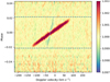 |
Fig. 5 Mean line profile tomography. The average stellar line has been removed, but not the systemic velocity. The Doppler shadow (red excess) and the atmospheric trace (blue absorption, plotted by the dotted blue line) are visible in the residuals. |
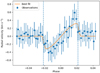 |
Fig. 6 RV residuals show the atmospheric RML effect. The overplotted orange line shows the best-fit RML model. |
5 Atmospheric trace
We studied the planetary atmospheric trace following the same strategy as with the RVs in Sect. 4, and applying it to the mean line profiles. We combined all five transits in order to increase the strength of the atmospheric signal and to average out spurious variations due to instrumental or telluric effects.
We averaged all our out-of-transit mean line profiles to obtain a purely stellar mean line profile. Because KELT-20 does not show any significant stellar variations either due to activity or pulsations, we were then able to remove the stellar component from our data simply by dividing each mean line profile (both in and out of transit) by the average out-of-transit stellar mean line profile. We then normalised the residuals by dividing them using two different linear fits, one for the points outside the stellar line limits, and the other for the points inside the stellar line limits. The latter fit was made avoiding the regions with Doppler shadow or the atmospheric trace. The resulting residuals are shown in Fig. 5. To enhance the signal visibility, they are binned with a 0.002 phase bin and a 1 km s−1 RV bin.
To isolate and investigate possible variations of the atmospheric trace during transit, we had to remove the Doppler shadow. To ensure that the removal process did not affect our analysis, we proceeded in two different ways that we describe below.
(a) We followed the method of Hoeijmakers et al. (2019) to select the residuals in which the Doppler shadow signal is far from the atmospheric trace and fitted it with a Gaussian. Then we fitted the Gaussian parameters with a second-order polynomial, so that the fit parameters of the Doppler shadow varied smoothly during the transit. We then removed the Doppler shadow Gaussian model from all the residuals.
We note here that we obtained better removals by first shifting all our data in the reference frame of the Doppler shadow, probably because of the geometry of the KELT-20 system. We did this using the estimated Doppler shadow RV obtained from Eq. (2) (Cegla et al. 2016),
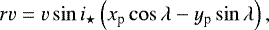 (2)
(2)
where
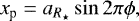
with λ the projected obliquity in radians,  the semi-major axis in units of stellar radius, ϕ the orbital phase, and i the orbital inclination in radians. After this, the signal of the Doppler shadow was vertically aligned, and we proceeded with the removal as described above.
(b) We adopted and adjusted the method from Cabot et al. (2020). The original method was applied to the UHJ WASP-121b, which orbits its host star in a near-polar orbit ( deg; Delrez et al. 2016). Because of this, its Doppler shadow in the stellar reference frame is almost completely vertically aligned at the centre of the stellar line profile. Cabot et al. (2020) removed it by fitting a third-degree polynomial on each column of the tomography in which the Doppler shadow fell.
Because the geometry of the KELT-20 system is different, we had to modify this approach to suit our data. First of all, we shifted the data in the reference frame of the Doppler shadow as in the original work of Cabot et al. (2020). We were then able to fit the columns in which the signal of the Doppler shadow fell, and finally, we divided each column by its fit. We used a fifth-degree polynomial instead of the original third-degree polynomial because it removed the Doppler shadow better.
We obtained two datasets in this way. Dataset A, in which the Doppler shadow was removed by Gaussian fitting, and dataset B, in which the Doppler shadow was removed by adapting the Cabot et al. (2020) method. Because the results we obtained with the two datasets agree well, we show here only the work done on dataset A, while the results from dataset B are presented in Appendix A.
After we removed the Doppler shadow signal, we shifted the dataset in the planet reference frame. We shifted each spectrum by the combination of VSys and the planet theoretical orbital RV (the barycentric correction was already applied by the HARPS-N DRS) in order to align the atmospheric signal in a vertical position around 0 km s−1 and to better study its variations (see Fig. 7). The planetary orbital RVs were computed for each epoch with the KeplerEllipse class of the PyAstronomy package using the orbital values of semi-major axis a, period P, eccentricity e, and inclination i from Table 1. This yields a Kp of 169 ± 6 km s−1, which is compatible with the values found in the literature (Casasayas-Barris et al. 2019; Nugroho et al. 2020; Stangret et al. 2020).
We then considered each mean line profile to map the velocity variations during transit. Because the atmospheric signal is weak, we applied a Savitzky-Golay filter (Savitzky & Golay 1964) to each profile in order to smooth out the noise and increase the signal visibility. The Savitzky-Golay filter works by computing a least-squares low-degree polynomial fit (third degree in our case) in a moving window on the data to estimate the value of the central point of each window, and it is able to smooth the data without greatly distorting the signal. While it was originally created for spectroscopic chemistry, the Savitzky-Golay filter has been successfully applied to several types of spectroscopic astronomical data (e.g. Deetjen 2000; Dimitriadis et al. 2019; Fleig et al. 2008). We applied the Savitzky-Golay filter by using the savgol_filter function of SciPy5 with an optimal window width of 15 pixel. We obtained the window value by applying the method proposed by Sadeghi & Behnia (2018) to our data. In Appendix B we show the results of the atmospheric analysis on the unfiltered dataset A to highlight the improvements obtained using the filter. The overall behaviour of the signal isclearly the same, but the uncertainties on the estimated values are much lower using the filtered data.
After applying the Savitzky-Golay filter, we fitted the atmospheric signal with a Markov chain Monte Carlo (MCMC) sampling and a correlated noise model using Gaussian processes with a Matérn-3/2 covariance kernel. In order to do this, we used the Python packages emcee6 (Foreman-Mackey et al. 2013)and george7 for the noise model. The priors on full width at half maximum (FWHM), RV, and depth were estimated as an average of the Gaussian fits on the different datasets, with broader widths than the expected uncertainties: FWHM = 20 ± 20 km s−1, RV = − 5 ± 20 km s−1, and the initial depth is computed on each dataset as depth=minimum-maximum and ranges from 3 × depth to 0.1 (to account for normalisation problems). In Fig. 8 we show 24 random posteriors for each of the 20 mean line profile residuals that we have during the transit.
The fit results are shown in Fig. 9. The 0.50, 0.16, and 0.84 quantiles of the posteriors distribution are used as the best values and the upper and lower 1σ uncertainties, respectively. The RV signal remain stable for most of the transit, and then it becomes blueshifted during egress. Except for one outlier, the FWHM is more stable. Although it appears to be lower during ingress, there is no statistically evident variation from the mean. The depth of the signal increases from the beginning to the centre of the transit, and then it decreases in a roughly symmetric way, with some points differing more than 1σ from the mean during ingress and egress (a flatter atmospheric signal), and in the middle of the transit (a deeper signal). In all cases, the variations (if any) are mainly found either during ingress, egress, or both.
Averaging the residuals in the first and second half of the transit (phases [−0.02:0.0] and [0.0:0.02], see Fig. 10) shows a higher FWHM value in the first half of the transit, but the result is not statistically significant. The depth variation is cancelled out within 1σ, and also the RV variation in the averaged signals disappears within 1σ because the main RV variation is caused only by the last three points (and the last point in particular), where the atmospheric signal is weaker (see the last panels of Fig. 8), and their contribution to the average is therefore lower.
We tried to study the atmospheric trace behaviour in each transit, but the S/N was too low to allow us to follow the finer variations that are already difficult to see in Fig. 9. However, we were able to determine the overall variations between the first andsecond half of the transits, and we found interesting results (see Fig. 11). The signal depth is stable in all transits except for night 4, where it decreases from the first to the second half of the transit. The FWHM show variations around 3σ level in the last two transits (4 and 5), and just above 1σ during transit 2. In all these three nights, the FWHM decreases from the first to the second half of the transit. It may be interesting to note that the FWHM shows indications of decreasing in transit 3 as well and of increasing in transit 1, but in both cases the variations are not statistically significant. Lastly, the RV variations are visible only in the last two transits (4 and 5), where the atmospheric signal shows a weak but significant redshift.
Even if the FWHM decrease found in our data is not repeated in the same way and with the same strength in every transit, it is still worthwhile to investigate some possible causes of this behaviour. It is interesting to note that a significant variation in FWHM has been found between the elements detected in the atmosphere of KELT-20b by Hoeijmakers et al. (2020), varying from 5.31 ± 0.99 km s−1 for CrII to 33.45 ± 3.30 km s−1 for MgI. Because our planetary atmospheric trace is obtained through the use of a stellar mask (where several different elements are combined), one possible interpretation for our FWHM variations might be a variable contribution of the chemical elements during the transit, for example due to temperature variations that may cause some of them to condense. Still, because FeIand FeII constitute more than half of the mask lines, another possible cause may be the condensation of iron, similarly to what occurs in the UHJ WASP-76b (Ehrenreich et al. 2020). Another interpretation could be the presence of more turbulent atmospheric conditions in the first part of the transit, for example due to a day- to night-side wind, as was also found in WASP-76b (Ehrenreich et al. 2020) and WASP-121b (Bourrier et al. 2020).
We stress here that the atmospheric RV variations of KELT-20b are not visible when only the first and second half of the transit are studied, even when all five transit datasets are combined (see Figs. 10 and 11), but they are slightly more visible when the finer atmospheric variations are traced (see Figs. 8 and 9). Because the signal is faint, this study is possible only in the combined data.
 |
Fig. 7 Line profile residuals after removing the Doppler shadow and after shifting in the planet reference frame. The atmospheric trace is clearly visible and centred around 0 km s−1. |
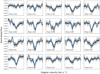 |
Fig. 8 Atmospheric signal found in the line profile residuals and the relative MCMC posteriors. All the graphics have the same abscissa (RVs from −40 to 40 km s−1) and ordinate (normalised flux from 0.998 to 1.001) to better follow the evolution of the signal. The graphics extend from phase −0.019 (upper left panel) to phase 0.019 (lower right panel) with a 0.002 phase step. |
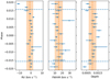 |
Fig. 9 RVs, FWHM, and depth of the atmospheric signal shown in Fig. 8 during transit. The vertical dashed orange lines and shaded areas show the mean values and relative standard deviation for each of the three quantities. All the data lie between t0 (start of ingress) and t1 (end of egress), while the horizontal dashed blue lines indicate t2 (end of ingress) and t3 (start of egress). |
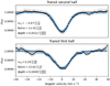 |
Fig. 10 Averaged atmospheric signal found in the line profile residuals in the first (phase [−0.02:0.0]) and second part (phase [0.0:0.02]) of the combined transits with the relative fit. |
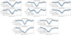 |
Fig. 11 Averaged atmospheric signal found in the line profile residuals in the first (phase [−0.02:0.0]) and second part (phase [0.0:0.02]) of each transit. From top left to bottom right: graphics show the results for transits 1, 2, 3, 4, and 5. |
6 Cross-correlation with FeI models
Nugroho et al. (2020) detected several elements in the atmosphere of KELT-20b through the CCF method, and they found a peculiar double-peak shape in the Kp − ΔV maps of FeI. The peaks have similar Kp, and they are roughly ≈10 km s−1 apart. The secondary blueshifted peak is weaker than the primary. The authors reconstructed the observed structure by simulating two FeI signals with different amplitudes and ΔV, and found the best match when the weaker signal (at ΔV = −10 km s−1) was masked from phase −0.01 and −0.016, simulating a delay in its appearance. This behaviour closely resembled what we observed in the planetary atmospheric RV variations, with a blueshifted signal in the final part of the transit (see Fig. 9).
Because they used the same HARPS-N observations as we did for our first three transits and we have two additional HARPS-N nights that were not used in their work, we decided to search for the same double-peak signature in our data. We were unable to use our LSD results directly because the stellar mask contains several different elements in addition to FeI, therefore we decided to apply the CCF method to obtain our own Kp − ΔV maps.
To create our model, we employed the πη line-by-line radiative transfer code (Ehrenreich et al. 2006, 2012; Pino et al. 2018). This code has been used for the simultaneous interpretation of HARPS high-resolution spectroscopic observations and HST WFC3 observations (Pino et al. 2018). For this paper, we updated the code to include line opacities from FeI and a continuum by H− following Pino et al. (2020), and equilibrium chemistry calculations for FeI and H− to calculate their volume-mixing ratios throughout the atmosphere. The FeI lines were taken from the VALD3 database8 and modelled as Voigt profiles. We accounted for thermal and natural broadening. We employed the publicly available FastChem code version 2 (Stock et al. 2018) for the equilibrium chemistry calculations.
We employed the fixed-temperature profile from Lothringer & Barman (2019) that is representative for a Teq = 2250 K planet orbiting an F0-type star (T⋆ = 7200 K). The other parameters employed in our model are R⋆, Mp, log VMRFe, and Rp at a reference pressure level of 10 bar (see Table 1). Nugroho et al. (2020) demonstrated that the neutral iron lines in KELT-20b can be well represented with a hydrostatic equilibrium model, provided that the model accounts for a scale factor (α in their notation). Our cross-correlation scheme is not sensitive to this scale factor, which we therefore fixed to 1.
Because we now directly investigated the planetary signal and were no longer interested in the stellar contribution that we used to study the classical and atmospheric RML, we prepared our data in a different way than for the LSD analysis. We started again from the whole spectra, including the regions that we cut out in Sect. 3. We then removed the out-of-transit stellar master and telluric contamination, and we performed a cross-correlation in the stellar restframe between the data and our model for each residual spectrum (as in Borsa et al. 2021). Our CCFs are defined as in Eq. (3),
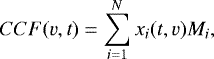 (3)
(3)
where x are the N wavelengths of the spectra taken at the time t and shifted at the velocity v, and M is the model normalised to unity. We imposed that all the model values lower than 5% of the maximum absorption line in the considered wavelength range were zero (e.g. Hoeijmakers et al. 2019).
We selected a step of 1 km s−1 and a velocity range [−200, 200] km s−1. The spectra were divided into segments of 200 Å (e.g. Hoeijmakers et al. 2019), and the cross-correlation was then performed for each segment. We masked the wavelength range 5240–5280 Å, which is heavily affected by telluric contamination. Then for each exposure we applied a weighted average between the CCFs of the single segments, where the weights applied to each segment were the sum of the depths of the lines in the model and the inverse of the standard deviation of the segment (i.e. the higher the S/N, the larger the weight). We then averaged all the in-transit CCFs after shifting them in the planetary restframe for a range of Kp values from 0 to 300 km s−1 in steps of 1 km s−1. The shift was performed by subtracting the planetary RV calculated for each spectrum as vp = Kp × sin2πϕ, where ϕ is the orbital phase. As a last step, we subtracted the VSys from all the averaged CCFs to obtain the Kp − ΔV maps. We then created S/N maps by computing the standard deviation of each Kp − ΔV map far from the planetary signal (i.e. excluding the region from VSys = −40 km s−1 to VSys = 40 km s−1), and then divided the Kp − ΔV maps by these values.
Our results are shown in Fig. 12. We identified the strongest peak or peaks in each map with a local maximum algorithm. We found the double-peak feature quite clearly in the first two transits, while only the weaker blueshifted signal is present in transit 3. In transits 4 and 5, only the stronger signal is visible. We recall that we analysed the same data as Nugroho et al. (2020) for transits 1, 2, and 3.
To further investigate the variability of the FeI signal as a function of transit, we ran MCMC simulations with the Python emcee package and drove their evolution by the likelihood scheme of Brogi & Line (2019). The CCF defined in Eq. (3) that is commonly used in stellar RVs is called cross-covariance in statistics. Compared to the statistical cross-correlation, it misses a normalisation factor that would force the CCF between −1 (perfect anti-correlation) and +1 (perfect correlation). The quantity in Eq. (3) is thus exactly the same as the cross-covariance R defined in Eq. (9) of Brogi & Line (2019) that was used for the MCMC simulations. However, the likelihood function of Brogi & Line (2019) contains additional terms, namely the data and model variances, which give information about the shape and amplitude of spectral lines. We also note that that the cross-correlation maps in Fig. 12 are converted into S/N by dividing by the standard deviation far from the peak. If we had used the full statistical formula for the cross-correlation, we would have obtained the same S/N, except for second-order variations of the model variance as a function of VSys and Kp.
We chose to present both analyses because the CCF approach is less sensitive to the modelling and thus more appropriate to capturing the initial detection of FeI even with an approximate template or a binary mask. The CCFs can also be compared with the existing literature. However, the likelihood approach allows us to better constrain the parameter space and explore the statistical evidence for night-to-night variability, and thus we opted for presenting both analyses.
In our simulations, the likelihood was maximised as a function of four parameters: the two velocities (orbital and systemic), the FWHM of the line profile, and the logarithm of a scaling factor, log S. While the measured systemic velocity is consistent within 1σ between the nights (except for the first night), the other three parameters show a clear variability, as reported in Table 3. Here we redefine Kp as Kp+atmo because it combines the projected orbital velocity of the planet and a contribution from the atmosphere physics and dynamics. With this more refined method we found no evidence of the double-peak structure. In Fig. 13 we show the corner plot of the posterior distribution found for transit night 2, where the double-peak structure is instead clearly visible in Fig. 12. We also investigated the combined data by fixing the FWHM and log S to their best-fitting values for each night and then running an additional MCMC with the five nights combined. This further test did not confirm a possible double solution either. The posterior in Kp+atmo instead appears to be single-peaked and centred at an intermediate value of 142 km s−1. The new results instead show that the values of Kp+atmo and logS are variable over some of the transits. Only the last two transits (4 and 5) yield a Kp+atmo value that is fully compatible with the theoretical Kp estimated in Sect. 5, while in the other transits and the combined data, Kp+atmo is systematically lower than the theoretical 169 ± 6 km s−1 value.
These results indicate that the dynamics probed by the FeI signal, as well as the overall strength of the iron lines, may change from transit to transit. Furthermore, there is some evidence that the broadening of the line profile also varies, as shown by the retrieved FWHM values, even if these variations are not strongly statistically significant. We note, however, that comparing these results with those of Sect. 5, the nights with larger Kp+atmo (4 and 5) are those with the larger FWHM variations of the atmospheric trace between the two halves of the transit, while night 1 has the more deviant values and is also the only night in which the atmospheric trace shows a possible increase in FWHM from the first to the second half of the transit (see Fig. 11). The difference between the FWHM values found here and those of the atmospheric trace may arise from the fact that the atmospheric trace described in Sect. 5 is caused by a combination of the different elements found in the stellar mask. Additionally, we confirm the blueshift of the FeI signal that was also found in the literature (Stangret et al. 2020; Hoeijmakers et al. 2020; Nugroho et al. 2020).
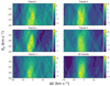 |
Fig. 12 Contour plots of the Kp − ΔV maps obtained from the cross-correlation of the residual spectra with the planetary FeI model. All the five transit nights and the combined data (bottom right panel) are shown. The prominent peaks are indicated with stars. |
Signal position, width, and model scale factor found with the MCMC simulations and the likelihood from Brogi & Line (2019).
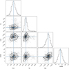 |
Fig. 13 Corner plot of the posterior distribution found with MCMC simulations and the Brogi & Line (2019) likelihood for transit 2, where the double-peak structure is clearer in the Kp − ΔV contour maps. No evidence of this structure is found here. |
7 Conclusions
Because of its high Teq (2260 ± 50 K), the atmospheric spectrum of the ultra-hot Jupiter KELT-20b correlates with the stellar mask that is used to compute the host star mean line profiles. We were thus able to detect and characterise the atmospheric RML effect in the stellar RV time-series, which resulted in an estimation of the size of the planetary atmosphere that correlates with the mask (Rp+atmo∕Rp = 1.13 ± 0.02). This agrees with literature values from metal line-depths, confirming the reliability of the atmospheric RML method. In addition, we were able to isolate the atmospheric trace in the mean line profile tomography. The high-resolution and high S/N of our data allowed us to fit the atmospheric signal and follow its variations during the transit.
We found possible variations of RV, FWHM, and depth of the atmospheric signal during the combined transit data and a different behaviour during different transits. The FWHM decreases during two transits, and decreases just above 1σ level during a third transit, while in another transit and in the combined data the measured decrease may be present, but it is not statistically significant. This possible greater FWHM spread during the first part of the transit may indicate turbulent conditions that becomemore stable in the second part of the transit. This behaviour resembles that found by Ehrenreich et al. (2020) in WASP-76b and by Bourrier et al. (2020) in WASP-121b, and it confirms the existence of different structures between morning and evening terminators, as suggested by Hoeijmakers et al. (2020). These authors analysed only one transit, and so they were unable to exclude a spurious nature for the RV variability. Another possible interpretation of the FWHM variations may be a variable contribution of elements to the overall atmospheric signal during the transit. Because the stellar mask contains different elements, all of them contribute to the resulting atmospheric trace, but their relative abundances may change during the transit due to temperature variations that may cause some of them to condense, for example. This may result in a FWHM variation due to the significant FWHM differences between the elements detected in the atmosphere of KELT-20b (Hoeijmakers et al. 2020). Because more than half of the stellar masklines are FeI and FeII lines, the condensation of iron (Ehrenreich et al. 2020) may play a role in this situation.
The RV variations are more visible in the combined data of the atmospheric trace, which confirms the atmospheric dynamics with a blueshift of the signal during egress. These RV variations led us to explore the results from Nugroho et al. (2020), who found a double-peak feature in their FeI Kp − ΔV maps. This feature consisted of a primary peak at ΔV = 0 km s−1 and a weaker secondary peak at ΔV = −10 km s−1. Their best match with simulated signals indicated a delayed appearance of the weaker blueshifted signal, which agrees well with the blueshift we found in the second part of the transit. The atmospheric trace that we studied in Sect. 5 was found in the mean line profiles obtained using the LSD software with a stellar mask suited for the host star KELT-20, and we were therefore unable to directly compare our results with those of Nugroho et al. (2020). We decided then to create our own Kp − ΔV maps using the standard cross-correlation method with a planetary atmospheric FeI model. Initially, we found the same double-peak structure in transits 1 and 2 with a simple contour analysis, but a more refined study using MCMC simulations driven by the likelihood scheme of Brogi & Line (2019) showed only a single significant peak per night. Nevertheless, we found some indication of the variability of the signal from one transit to another, which aligns well with the tentative results from the line profile tomography.
To conclude, we used different methods (line profile tomography and FeI CCFs) to search independently for variability in the atmospheric signal of KELT-20b. We found an indication that the FWHM and RV varied during some of the transits. We also confirm the blueshift of the FeI signal and the reliability of the atmospheric RML method for estimating the atmospheric extension.
Acknowledgements
This work has made use of the VALD3 database, operated at Uppsala University, the Institute of Astronomy RAS in Moscow, and the University of Vienna. M.B. acknowledges support from the UK Science and Technology Facilities Council (STFC) research grant ST/S000631/1. G.Sc. acknowledges the funding support from Italian Space Agency (ASI) regulated by “Accordo ASI-INAF n. 2013-016-R.0 del 9 luglio 2013 e integrazione del 9 luglio 2015”. F.B. acknowledges support from PLATO ASI-INAF agreement n. 2015-019-R.1-2018. The research leading to these results has received funding from the European Research Council (ERC) under the European Unions Horizon 2020 research and innovation programme (grant agreement no. 679633, Exo-Atmos). This research used the facilities of the Italian Center for Astronomical Archive (IA2) operated by INAF at the Astronomical Observatory of Trieste.
Appendix A Atmospheric trace analysis of dataset B
In order to ensure that the removal of the Doppler shadow did not unduly affect the study of the atmospheric trace, we performed the removal with two methods, which generated two datasets. While the results from dataset A are shown in the paper, we show here the same analysis performed on dataset B.
The line profile residuals after the Doppler shadow was removed were shifted in the planetary reference frame and are shown in Fig. A.1). It is clear that the Doppler shadow removal was less efficient in this case than in dataset A (see Fig. 7), as is shown by the large residuals left in the tomography. We then smoothed each in-transit residual by applying a third-degree Savitzky-Golay filter with a 15-pixel window, and we fitted the atmospheric signal using an MCMC with a correlated noise model.
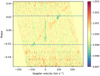 |
Fig. A.1 Dataset B: line profile residuals after removing the Doppler shadow and after shifting in the planet reference frame. The atmospheric trace is clearly visible and centred around 0 km s−1. The Doppler shadow residual is still visible. |
The resulting RVs, FWHMs, and depths are shown in Fig. A.2. As for dataset A, we found a blueshift during egress, while the FWHM is more stable (except for the same outlier as found in dataset A), and the depth shows a symmetric increase andsubsequent decrease during transit.
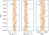 |
Fig. A.2 RVs, FWHM and depth of the atmospheric signal during transit using dataset B: the vertical dashed orange lines and shaded areas show the mean values and relative standard deviation for each of the three quantities. All the data are comprised between t0 (start of ingress) and t1 (end of egress), while the horizontal dashed blue lines indicate t2 (end of ingress) and t3 (start of egress). |
We studied the overall variations during transit by averaging all residuals in the first and second half of the transit (phases [−0.02:0.0] and [0.0:0.02]), see Fig. A.3.
 |
Fig. A.3 Averaged atmospheric signal in the first (phase [−0.02:0.0]) and second part (phase [0.0:0.02]) of the transit with relative fit using dataset B. |
We also performed the same study on each individual night (see Fig. A.4). We found mostly the same results as for dataset A. The atmospheric depth is stable in all transit nights (during night 4, the variation also falls exactly at the 1σ level), the RV variations are statistically significant only in night 4, where a weak redshift is visible, and the FWHM decreases during the transit in nights 2 (just above the 1σ level), 4, and 5 (around the 3σ level). The results are qualitatively identical to those obtained with dataset A, showing that the choice of method for removing the Doppler shadow does not affect our work.
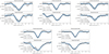 |
Fig. A.4 Averaged atmospheric signal in the first (phase [−0.02:0.0]) and second part (phase [0.0:0.02]) of each transit using dataset B. From top left to bottom right: graphics show the results for nights 1, 2, 3, 4, and 5. |
Appendix B Atmospheric trace analysis of the unfiltered dataset A
We performed the same analysis as shown in Sect. 5 on the unfiltered dataset A, combining all five transits. While the atmospheric trace signal is much noisier, the overall behaviour of its FWHM, RV, and depth, shown in Fig. B.1, closely resembles that found in the filtered data (Fig. 9), as can be seen from the direct comparison shown in Fig. B.2.
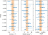 |
Fig. B.1 RVs, FWHM, and depth of the atmospheric signal during transit using the unfiltered data. The vertical dashed orange lines and shaded areas show the mean values and relative standard deviation for each of the three quantities. All the data lie between t0 (start of ingress) and t1 (end of egress), while the horizontal dashed blue lines indicate t2 (end of ingress) and t3 (start of egress). |
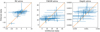 |
Fig. B.2 Comparison of the atmospheric trace values of RV, FWHM, and depth found in dataset A using the unfiltered data (x-axis) and filtered data (y-axis). The orange lines show the one-to-one correlation. |
The overall variations during the transit (Fig. B.3), arising from comparing the atmosphericsignal in the first and second half of the transit, are also similar to those found in the filtered data (Fig. 10). For example, in the unfiltered data, the FWHM decreases from 16.25 to 14.24
 km s−1, while in the filtered data, it decreases from 15.62
 to 13.76
 km s−1. In both cases, the decrease amounts to ≈ 2 km s−1, while the slightly higher FWHM values found in the unfiltered dataset may be due to the excess noise.
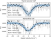 |
Fig. B.3 Averaged atmospheric signal in the first (phase [−0.02:0.0]) and second part (phase [0.0:0.02]) of the transit with relative fit using the unfiltered data. |
We can reliably confirm that the Savitzky-Golay filter behaves as expected. It preserves the signal behaviour and decreases the uncertainties because the noise is removed.
References
- Asplund, M., Grevesse, N., Sauval, A. J., & Scott, P. 2009, ARA&A, 47, 481 [NASA ADS] [CrossRef] [Google Scholar]
- Bell, T. J., & Cowan, N. B. 2018, ApJ, 857, L20 [Google Scholar]
- Borsa, F., Rainer, M., Bonomo, A. S., et al. 2019, A&A, 631, A34 [NASA ADS] [CrossRef] [EDP Sciences] [Google Scholar]
- Borsa, F., Allart, R., Casasayas-Barris, N., et al. 2021, A&A, 645, A24 [EDP Sciences] [Google Scholar]
- Bourrier, V., Ehrenreich, D., Lendl, M., et al. 2020, A&A, 635, A205 [NASA ADS] [CrossRef] [EDP Sciences] [Google Scholar]
- Brogi, M., & Line, M. R. 2019, AJ, 157, 114 [Google Scholar]
- Cabot, S. H. C., Madhusudhan, N., Welbanks, L., Piette, A., & Gandhi, S. 2020, MNRAS, 494, 363 [NASA ADS] [CrossRef] [Google Scholar]
- Casasayas-Barris, N., Pallé, E., Yan, F., et al. 2018, A&A, 616, A151 [NASA ADS] [CrossRef] [EDP Sciences] [Google Scholar]
- Casasayas-Barris, N., Pallé, E., Yan, F., et al. 2019, A&A, 628, A9 [NASA ADS] [CrossRef] [EDP Sciences] [Google Scholar]
- Cegla, H. M., Lovis, C., Bourrier, V., et al. 2016, A&A, 588, A127 [NASA ADS] [CrossRef] [EDP Sciences] [Google Scholar]
- Claudi, R., Benatti, S., Carleo, I., et al. 2016, Proc. SPIE Conf. Ser., 9908, 99081A [Google Scholar]
- Cosentino, R., Lovis, C., Pepe, F., et al. 2012, Proc. SPIE Conf. Ser., 8446, 84461V [CrossRef] [Google Scholar]
- Cosentino, R., Lovis, C., Pepe, F., et al. 2014, Proc. SPIE Conf. Ser., 9147, 91478C [Google Scholar]
- Covino, E., Esposito, M., Barbieri, M., et al. 2013, A&A, 554, A28 [NASA ADS] [CrossRef] [EDP Sciences] [Google Scholar]
- Czesla, S., Schröter, S., Schneider, C. P., et al. 2019, PyA: Python astronomy-related packages. Astrophys. Source Code Libr. [record ascl:1906.010] [Google Scholar]
- Deetjen, J. L. 2000, A&A, 360, 281 [NASA ADS] [Google Scholar]
- Delrez, L., Santerne, A., Almenara, J. M., et al. 2016, MNRAS, 458, 4025 [Google Scholar]
- Dimitriadis, G., Rojas-Bravo, C., Kilpatrick, C. D., et al. 2019, ApJ, 870, L14 [Google Scholar]
- Donati, J. F., Semel, M., Carter, B. D., Rees, D. E., & Collier Cameron, A. 1997, MNRAS, 291, 658 [NASA ADS] [CrossRef] [MathSciNet] [Google Scholar]
- Dravins, D., Lindegren, L., & Torkelsson, U. 1990, A&A, 237, 137 [NASA ADS] [Google Scholar]
- Ehrenreich, D., Tinetti, G., Lecavelier Des Etangs, A., Vidal-Madjar, A., & Selsis, F. 2006, A&A, 448, 379 [NASA ADS] [CrossRef] [EDP Sciences] [Google Scholar]
- Ehrenreich, D., Vidal-Madjar, A., Widemann, T., et al. 2012, A&A, 537, L2 [NASA ADS] [CrossRef] [EDP Sciences] [Google Scholar]
- Ehrenreich, D., Lovis, C., Allart, R., et al. 2020, Nature, 580, 597 [Google Scholar]
- Fleig, J., Rauch, T., Werner, K., & Kruk, J. W. 2008, A&A, 492, 565 [NASA ADS] [CrossRef] [EDP Sciences] [Google Scholar]
- Foreman-Mackey, D., Hogg, D. W., Lang, D., & Goodman, J. 2013, PASP, 125, 306 [Google Scholar]
- Gray, D. F. 2008, The Observation and Analysis of Stellar Photospheres (Cambridge: Cambridge University Press) [Google Scholar]
- Guilluy, G., Andretta, V., Borsa, F., et al. 2020, A&A, 639, A49 [EDP Sciences] [Google Scholar]
- Heng, K., & Showman, A. P. 2015, Ann. Rev. Earth Planet. Sci., 43, 509 [NASA ADS] [CrossRef] [Google Scholar]
- Hoeijmakers, H. J., Ehrenreich, D., Heng, K., et al. 2018, Nature, 560, 453 [NASA ADS] [CrossRef] [Google Scholar]
- Hoeijmakers, H. J., Ehrenreich, D., Kitzmann, D., et al. 2019, A&A, 627, A165 [NASA ADS] [CrossRef] [EDP Sciences] [Google Scholar]
- Hoeijmakers, H. J., Cabot, S. H. C., Zhao, L., et al. 2020, A&A, 641, A120 [EDP Sciences] [Google Scholar]
- Høg, E., Fabricius, C., Makarov, V. V., et al. 2000, A&A, 355, L27 [Google Scholar]
- Lothringer, J. D., & Barman, T. 2019, ApJ, 876, 69 [Google Scholar]
- Lund, M. B., Rodriguez, J. E., Zhou, G., et al. 2017, AJ, 154, 194 [NASA ADS] [CrossRef] [Google Scholar]
- McLaughlin, D. B. 1924, ApJ, 60, 22 [Google Scholar]
- Nugroho, S. K., Gibson, N. P., de Mooij, E. J. W., et al. 2020, MNRAS, 496, 504 [Google Scholar]
- Ohta, Y., Taruya, A., & Suto, Y. 2005, ApJ, 622, 1118 [Google Scholar]
- Oliva, E., Origlia, L., Maiolino, R., et al. 2012, Proc. SPIE Conf. Ser., 8446, 84463T [Google Scholar]
- Origlia, L., Oliva, E., Baffa, C., et al. 2014, Proc. SPIE Conf. Ser., 9147, 91471E [Google Scholar]
- Parmentier, V., Line, M. R., Bean, J. L., et al. 2018, A&A, 617, A110 [NASA ADS] [CrossRef] [EDP Sciences] [Google Scholar]
- Pino, L., Ehrenreich, D., Wyttenbach, A., et al. 2018, A&A, 612, A53 [NASA ADS] [CrossRef] [EDP Sciences] [Google Scholar]
- Pino, L., Désert, J.-M., Brogi, M., et al. 2020, ApJ, 894, L27 [Google Scholar]
- Piskunov, N. E., Kupka, F., Ryabchikova, T. A., Weiss, W. W., & Jeffery, C. S. 1995, A&AS, 112, 525 [Google Scholar]
- Rainer, M., Poretti, E., Mistò, A., et al. 2016, AJ, 152, 207 [NASA ADS] [CrossRef] [EDP Sciences] [Google Scholar]
- Reiners, A., & Schmitt, J. H. M. M. 2002, A&A, 384, 155 [NASA ADS] [CrossRef] [EDP Sciences] [Google Scholar]
- Rossiter, R. A. 1924, ApJ, 60, 15 [Google Scholar]
- Ryabchikova, T., Piskunov, N., Kurucz, R. L., et al. 2015, Phys. Scr, 90, 054005 [Google Scholar]
- Sadeghi, M., & Behnia, F. ArXiv e-prints [arXiv:1808.10489] [Google Scholar]
- Savitzky, A., & Golay, M. J. E. 1964, Anal. Chem., 36, 1627 [Google Scholar]
- Smith, M. A.,& Gray, D. F. 1976, PASP, 88, 809 [NASA ADS] [CrossRef] [Google Scholar]
- Stangret, M., Casasayas-Barris, N., Pallé, E., et al. 2020, A&A, 638, A26 [CrossRef] [EDP Sciences] [Google Scholar]
- Stock, J. W., Kitzmann, D., Patzer, A. B. C., & Sedlmayr, E. 2018, MNRAS, 479, 865 [NASA ADS] [Google Scholar]
- Talens, G. J. J., Justesen, A. B., Albrecht, S., et al. 2018, A&A, 612, A57 [NASA ADS] [CrossRef] [EDP Sciences] [Google Scholar]
- Van Rossum, G., & Drake Jr, F. L. 1995, Python Tutorial (The Netherlands: Centrum voor Wiskunde en Informatica Amsterdam) [Google Scholar]
See Pino et al. (2020) for a full list of references for the case of FeI.
All Tables
Physical and orbital parameters of the KELT-20 system (also known as MASCARA-2 or HD 185603).
Signal position, width, and model scale factor found with the MCMC simulations and the likelihood from Brogi & Line (2019).
All Figures
|
Fig. 1 Mean line profile of a single KELT-20 spectrum obtained with the LSD software and Teff = 10 000 K (solid blue line) along with the rotational broadening fit (dash-dotted orange line). For comparison, the mean line profile of the same spectrum with the Teff = 9000 K is shown (dashed green line). The Doppler shadow of the planet is clearly visible as a bump in both lines. |
| In the text | |
|
Fig. 2 Systemic velocity of the five nights: a weak downward trend is clearly visible. |
| In the text | |
|
Fig. 3 RV data phase-folded using the known orbital period of KELT-20b (P = 3.474119 days). The RV values were shifted by the difference between the individual VSys of each night and the average VSys value to account for the trend found in our data. |
| In the text | |
|
Fig. 4 Comparison of the observed RVs averaged with 0.002 phase bin (blue points) and the RML RV model (orange line). The model appears to overestimate the amplitude of the RML effect because the atmospheric RML effect decreases the signal amplitude. The vertical dashed lines show the transit ingress and egress. |
| In the text | |
|
Fig. 5 Mean line profile tomography. The average stellar line has been removed, but not the systemic velocity. The Doppler shadow (red excess) and the atmospheric trace (blue absorption, plotted by the dotted blue line) are visible in the residuals. |
| In the text | |
|
Fig. 6 RV residuals show the atmospheric RML effect. The overplotted orange line shows the best-fit RML model. |
| In the text | |
|
Fig. 7 Line profile residuals after removing the Doppler shadow and after shifting in the planet reference frame. The atmospheric trace is clearly visible and centred around 0 km s−1. |
| In the text | |
|
Fig. 8 Atmospheric signal found in the line profile residuals and the relative MCMC posteriors. All the graphics have the same abscissa (RVs from −40 to 40 km s−1) and ordinate (normalised flux from 0.998 to 1.001) to better follow the evolution of the signal. The graphics extend from phase −0.019 (upper left panel) to phase 0.019 (lower right panel) with a 0.002 phase step. |
| In the text | |
|
Fig. 9 RVs, FWHM, and depth of the atmospheric signal shown in Fig. 8 during transit. The vertical dashed orange lines and shaded areas show the mean values and relative standard deviation for each of the three quantities. All the data lie between t0 (start of ingress) and t1 (end of egress), while the horizontal dashed blue lines indicate t2 (end of ingress) and t3 (start of egress). |
| In the text | |
|
Fig. 10 Averaged atmospheric signal found in the line profile residuals in the first (phase [−0.02:0.0]) and second part (phase [0.0:0.02]) of the combined transits with the relative fit. |
| In the text | |
|
Fig. 11 Averaged atmospheric signal found in the line profile residuals in the first (phase [−0.02:0.0]) and second part (phase [0.0:0.02]) of each transit. From top left to bottom right: graphics show the results for transits 1, 2, 3, 4, and 5. |
| In the text | |
|
Fig. 12 Contour plots of the Kp − ΔV maps obtained from the cross-correlation of the residual spectra with the planetary FeI model. All the five transit nights and the combined data (bottom right panel) are shown. The prominent peaks are indicated with stars. |
| In the text | |
|
Fig. 13 Corner plot of the posterior distribution found with MCMC simulations and the Brogi & Line (2019) likelihood for transit 2, where the double-peak structure is clearer in the Kp − ΔV contour maps. No evidence of this structure is found here. |
| In the text | |
|
Fig. A.1 Dataset B: line profile residuals after removing the Doppler shadow and after shifting in the planet reference frame. The atmospheric trace is clearly visible and centred around 0 km s−1. The Doppler shadow residual is still visible. |
| In the text | |
|
Fig. A.2 RVs, FWHM and depth of the atmospheric signal during transit using dataset B: the vertical dashed orange lines and shaded areas show the mean values and relative standard deviation for each of the three quantities. All the data are comprised between t0 (start of ingress) and t1 (end of egress), while the horizontal dashed blue lines indicate t2 (end of ingress) and t3 (start of egress). |
| In the text | |
|
Fig. A.3 Averaged atmospheric signal in the first (phase [−0.02:0.0]) and second part (phase [0.0:0.02]) of the transit with relative fit using dataset B. |
| In the text | |
|
Fig. A.4 Averaged atmospheric signal in the first (phase [−0.02:0.0]) and second part (phase [0.0:0.02]) of each transit using dataset B. From top left to bottom right: graphics show the results for nights 1, 2, 3, 4, and 5. |
| In the text | |
|
Fig. B.1 RVs, FWHM, and depth of the atmospheric signal during transit using the unfiltered data. The vertical dashed orange lines and shaded areas show the mean values and relative standard deviation for each of the three quantities. All the data lie between t0 (start of ingress) and t1 (end of egress), while the horizontal dashed blue lines indicate t2 (end of ingress) and t3 (start of egress). |
| In the text | |
|
Fig. B.2 Comparison of the atmospheric trace values of RV, FWHM, and depth found in dataset A using the unfiltered data (x-axis) and filtered data (y-axis). The orange lines show the one-to-one correlation. |
| In the text | |
|
Fig. B.3 Averaged atmospheric signal in the first (phase [−0.02:0.0]) and second part (phase [0.0:0.02]) of the transit with relative fit using the unfiltered data. |
| In the text | |
Current usage metrics show cumulative count of Article Views (full-text article views including HTML views, PDF and ePub downloads, according to the available data) and Abstracts Views on Vision4Press platform.
Data correspond to usage on the plateform after 2015. The current usage metrics is available 48-96 hours after online publication and is updated daily on week days.
Initial download of the metrics may take a while.