| Issue |
A&A
Volume 648, April 2021
The LOFAR Two Meter Sky Survey
|
|
|---|---|---|
| Article Number | A12 | |
| Number of page(s) | 13 | |
| Section | Catalogs and data | |
| DOI | https://doi.org/10.1051/0004-6361/202038896 | |
| Published online | 07 April 2021 | |
LOFAR Deep Fields: probing a broader population of polarized radio galaxies in ELAIS-N1
1
Faculty of Physics and Astronomy, Astronomical Institute, Ruhr University Bochum,
Universitätstrasse 150,
44801
Bochum,
Germany
e-mail: This email address is being protected from spambots. You need JavaScript enabled to view it.
2
School of Physical Sciences and Centre for Astrophysics & Relativity, Dublin City University,
Glasnevin,
D09 W6Y4, Ireland
3
INAF – Osservatorio Astronomico di Cagliari,
Via della Scienza 5,
09047
Selargius (CA), Italy
4
Ruđer Bošković Institute,
Bijenička cesta 54,
10000
Zagreb, Croatia
5
Astronomical Observatory, Jagiellonian University,
ul. Orla 171, 30-244
Kraków, Poland
6
Department of Space, Earth and Environment, Chalmers University of Technology, Onsala Space Observatory,
439 92
Onsala, Sweden
7
SUPA, Institute for Astronomy, Royal Observatory,
Blackford Hill,
Edinburgh,
EH9 3HJ, UK
8
CSIRO Astronomy and Space Science,
PO Box 1130,
Bentley,
WA
6102, Australia
9
ASTRON, the Netherlands Institute for Radio Astronomy,
Postbus 2,
7990 AA
Dwingeloo, The Netherlands
10
GEPI,
Observatoire de Paris, CNRS, Université Paris Diderot,
5 place Jules Janssen,
92190
Meudon, France
11
Centre for Radio Astronomy Techniques and Technologies, Department of Physics and Electronics, Rhodes University,
Grahamstown
6140, South Africa
12
USN, Observatoire de Paris, CNRS, PSL, UO,
Nançay, France
13
Centre for Astrophysics Research, University of Hertfordshire,
College Lane,
Hatfield
AL10 9AB, UK
14
Hamburger Sternwarte, Universität Hamburg,
Gojenbergsweg 112,
21029
Hamburg, Germany
15
INAF-IRA,
Via P. Gobetti 101,
40129
Bologna, Italy
Received:
11
July
2020
Accepted:
22
August
2020
Abstract
We present deep polarimetric observations of the European Large Area ISO Survey-North 1 (ELAIS-N1) field using the Low Frequency Array (LOFAR) at 114.9–177.4 MHz. The ELAIS-N1 field is part of the LOFAR Two-metre Sky Survey deep fields data release I. For six eight-hour observing epochs, we align the polarization angles and stack the 20″-resolution Stokes Q, U-parameter data cubes. This produces a 16 deg2 image with 1σQU sensitivity of 26 μJy beam−1 in the central area. In this paper, we demonstrate the feasibility of the stacking technique, and we generate a catalog of polarized sources in ELAIS-N1 and their associated Faraday rotation measures (RMs). While in a single-epoch observation we detect three polarized sources, this number increases by a factor of about three when we consider the stacked data, with a total of ten sources. This yields a surface density of polarized sources of one per 1.6 deg2. The Stokes I images of three of the ten detected polarized sources have morphologies resembling those of FR I radio galaxies. This represents a greater fraction of this type of source than previously found, which suggests that more sensitive observations may help with their detection.
Key words: polarization / galaxies: individual: ELAIS-N1 / radio continuum: galaxies / techniques: polarimetric
© ESO 2021
1 Introduction
The Low Frequency Array (LOFAR, van Haarlem et al. 2013) is a phased array radio interferometer, developed to explore the low-frequency radio sky (below 250 MHz). Because of its large field of view (>10 deg2 at 150 MHz), LOFAR is ideal for performing large-area sky surveys.
In addition to being a general purpose facility, LOFAR has been used to conduct several large key projects. These include studies of the Epoch of Reionization (EoR), deep extragalactic surveys, transient sources, ultra high energy cosmic rays, solar science and space weather, and cosmic magnetism.
The present project is carried out within the framework of the LOFAR Magnetism Key Science Project (MKSP1), which aims to study the magnetized Universe using LOFAR. Magnetic fields are ubiquitous throughout the Universe, and they play an important role in galaxy and galaxy cluster evolution as well as in the interstellar and intracluster media (e.g., Beck & Wielebinski 2013). The Faraday rotation measure (RM) quantifies the degree of rotation undergone by the polarization position angle, as a function of wavelength-squared, due to magneto-ionic media between the emitting source and the observer. Therefore, the RM provides information about magnetic fields along the line of sight (e.g., Han 2017). Catalogs of RMs of polarized radio sources can be used to study the Faraday rotation of our Galaxy and constrain its large-scale magnetic fields (e.g., Hutschenreuter & Enßlin 2020; Van Eck et al. 2011; Sobey et al. 2019). These catalogs are also powerful tools for the study of extragalactic large-scale magnetic fields, as shown by Bonafede et al. (2010), who determined the Coma cluster magnetic field strength from RMs. Moreover, due to the high sensitivity and high precision of new-generation radio interferometers, RM catalogs of polarized radio sources will be key components for the investigation of the magnetization of the cosmic web (e.g., Vacca et al. 2016; O’Sullivan et al. 2020).
Polarization observations can be used to investigate the emitting sources and the magneto-ionic media moving toward them by using Faraday rotation and frequency-dependent depolarization measurements (e.g., Burn 1966; Sokoloff et al. 1998). For example, different source populations can be distinguished and characterized (Farnes et al. 2014; Anderson et al. 2015). Two of the main science goals that are particularly relevant to deep field polarization observations are: (i) the study of galaxy evolution through the analysis of polarized source populations and the characterization of individual polarized sources; and (ii) to enlarge the database of extragalactic Faraday RMs used for the study of cosmic magnetism. Here, we present a catalog of polarized radio sources detected using LOFAR observations of the European Large Area ISO Survey-North 1 (ELAIS-N1) field, including their RMs and additional characteristics.
The ELAIS-N1 field was one of the regions observed by the ELAIS survey (Oliver et al. 2000) in the Northern Hemisphere (RA = 16h10m01s, Dec = 54°30′36′′). This survey was a single Open Time project conducted by the Infrared Space Observatory (ISO, Kessler et al. 1996). This field has exceptional multiwavelength coverage. It has been observed at X-ray (Manners et al. 2003), ultraviolet (Martin et al. 2005; Morrissey et al. 2007), optical (McMahon et al. 2001; Aihara et al. 2018), and infrared wavelengths (Lawrence et al. 2007; Lonsdale et al. 2003; Mauduit et al. 2012; Oliver et al. 2012). Kondapally et al. (2021) present a detailed description of the multiwavelength coverage of the field. At radio frequencies, the ELAIS-N1 field was observed with the Giant Metrewave Radio Telescope (GMRT) at 325 MHz (Sirothia et al. 2009) and at 610 MHz (Ocran et al. 2020). Chakraborty et al. (2019) observed it with the upgraded GMRT at 300–500 MHz. Sabater et al. (2021) present a comparison between these previous radio observations and our observations of the field. In addition, the ELAIS-N1 field has been covered by several large radio surveys, including the Westerbork Northern Sky Survey (WENSS, 325 MHz, Rengelink et al. 1997), the NRAO Very Large Array Sky Survey (NVSS, 1.4 GHz, Condon et al. 1998), and the Faint Images of the Radio Sky at Twenty Centimeters Survey (FIRST, 1.4 GHz, Becker et al. 1995; White et al. 1997).
Radio source counts are a useful tool for studying the evolution of radio source populations. They have been well studied in total intensity (e.g., Hopkins et al. 2003; Condon et al. 2012; Smolčić et al. 2017), but polarized radio source counts are under-explored, in particular at low frequencies and at sub-mJy flux densities. Polarized source counts probe the evolution of magnetic fields and, at low flux densities, are thought to be sensitive to properties of the various radio source populations in a different way than the total-intensity source counts, since different populations are expected to show different intrinsic polarization properties related to the different mechanisms of emission (Stil et al. 2009; Hardcastle et al. 1997; Laing & Bridle 2014). Taylor et al. (2007) presented polarimetric observations of the ELAIS-N1 field at 1.4 GHz. They imaged a region of 7.43 deg2 to a maximum sensitivity in Stokes Q and U of 78 μJy beam−1, and detected 83 polarized sources. Grant et al. (2010) presented an extension of that study, imaging a region of 15.16 deg2, also at 1.4 GHz, to a maximum sensitivity in Stokes Q and U of 45 μJy beam−1, and detected 136 polarized sources. They constructed the Euclidean-normalized polarized differential source counts down to 400 μJy and found that fainter radio sources have a higher fractional polarization than the brighter ones. This result was questioned by Hales et al. (2014a,b), who described the second data release of the Australia Telescope Large Area Survey (ATLAS) at 1.4 GHz and presented the 1.4 GHz Euclidean normalized differential number-counts from observations of the Chandra Deep Field-South (CDFS) and European Large Area Infrared Space Observatory Survey-South 1 (ELAIS-S1) regions. They found a smooth decline in both the total-intensity and linear polarization source counts from mJy levels down to ~100 μJy (their survey limit) and no signs of an anticorrelation between total-intensity and fractional polarization.
The precision in RM measurements largely depends on the span in wavelength-squared, λ2, and the sensitivity of the observations. Therefore, very-low-frequency observations allow us to measure Faraday depths very precisely (typical precision on the order of 0.1 rad m-2; see Brentjens & de Bruyn 2005). However, the degree of polarization of most sources decreases with decreasing frequency due to Faraday depolarization (Burn 1966). Bernardi et al. (2013) presented a Stokes I, Q, and U survey at 189 MHz with the Murchison Widefield Array (MWA; Tingay et al. 2013) covering 2400 deg2 and found that the polarization fraction of compact sources decreases at lower frequencies. Lenc et al. (2016) presented deep polarimetric observations at 154 MHz with the MWA, covering 625 deg2, and detected four extragalactic polarized sources. A follow-up wide-area MWA survey effort based on the GaLactic and Extra-Galactic All-Sky MWA (GLEAM) survey (Hurley-Walker et al. 2017), called the POlarization from the GLEAM Survey (POGS; Riseley et al. 2018), led to the detection of 81 sources in 6400 deg2 at 216 MHz, and 517 sources over the full southern sky at 169−231 MHz (Riseley et al. 2020). However, these studies have relatively low angular resolution (≈ 3−16 arcmin), which can make the detection of polarized sources at low frequencies even more challenging due to beam depolarization.
In general, recent developments in low-frequency radio interferometers and improvements in calibration techniques have enabled the detection of many extragalactic polarized sources. In particular, LOFAR has the potential to minimize the effect of beam depolarization with observations at higher angular resolution. Neld et al. (2018) developed a computationally efficient and rigorously defined algorithm to find linearly polarized sources in LOFAR data and applied it to previously calibrated data of the M51 field (Mulcahy et al. 2014). Van Eck et al. (2018) reported developments in polarization processing for the 570 deg2 preliminary data release region from the LOFAR Two-Metre Sky Survey (LoTSS2, Shimwell et al. 2017, 2019) and presented a catalog of 92 polarized radio sources at 150 MHz with 4.3-arcmin resolution and 1 mJy root mean square (rms) sensitivity. O’Sullivan et al. (2019) presented the Faraday RM and depolarization properties of a giant radio galaxy using LOFAR and demonstrated the potential of LOFAR to probe the weak signature of the intergalactic magnetic field (see also O’Sullivan et al. 2020).
In order to study magnetic fields in extragalactic sources, it is essential to reach similar sensitivity to the surveys at higher frequencies, but with higher precision in RM. This requires very deep observations at low frequencies, well below the thermal noise of a typical eight-hour LOFAR observing run. Therefore, in order to improve the signal-to-noise ratio (S/N) of our data and detect fainter sources, we tested and implemented a new stacking procedure to combine the Stokes Q and U data cubes obtained from several LOFAR observations.
Here, we present the methods and results using LOFAR images of a 16 deg2 area toward the ELAIS-N1 field. The structure of this paper is as follows. In Sect. 2, we give an overview of the radio polarization observations and of the data calibration process. The description of the stacking technique is presented in Sect. 3. In Sect. 4, we present our catalog and discuss the properties of the detected sources, and we summarize our findings in Sect. 5. Throughout this paper, we assume a flat Lambda cold dark matter (ΛCDM) cosmology with H0 = 67.4 km s−1 Mpc−1, ΩM = 0.315, and ΩΛ = 0.685 (Planck Collaboration VI 2020).
2 Observations and data processing
2.1 Observations
A polarimetric analysis of the ELAIS-N1 field with LOFAR was initially carried out as part of commissioning activities to characterize the LOFAR performance and the foregrounds in the LOFAR EoR fields (Jelić et al. 2014). Since then, significantly more data have been accumulated. Here we present observations of the ELAIS-N1 field, as part of the LoTSS Deep Field project. The LoTSS Deep Fields comprise substantially deeper observations of the four best-studied degree-scale extragalactic fields in the northern sky, with an ultimate aim of reaching an rms depth of ~10 μJy beam−1 over 30–50 deg2. The LoTSS Deep Fields first data release (Tasse et al. 2021; Sabater et al. 2021) comprises 100–200 h of data on each of three of these fields (ELAIS-N1, Lockman Hole and Boötes).
The observations of the ELAIS-N1 field used for this project were carried out with the LOFAR High Band Antenna (HBA) between May 2013 and August 2015 (cycles 0, 2, and 4; proposals LC0_019, LC2_024, and LC4_008). A total of 27 epochs, where an epoch is defined as an eight-hour LOFAR observation, were observed in full polarization. However, five data sets were excluded because of poor ionospheric conditions, noise levels, or data quality. This resulted in 22 available epochs and a total of 176 h of observations. The observations were followed by 5 to 10 min observations of 3C380, which was the source selected for the primary calibration process. For all epochs, the observations were centered at RA = 16h11m and Dec = 55°00′. A detailed description of the observations can be found in Sabater et al. (2021).
In this paper, we only used six epochs for testing purposes and to validate our new procedures on a representative subset of the available data. The Stokes Q and U data cubes each have 640 frequency channels with a channel width of 97.7 kHz, covering a frequency range from 114.9 to 177.4 MHz. The imaged region covers an area of 16 deg2. The identification numbers of the selected epochs used here are: 020, 024, 027, 028, 030, and 031. The other epochs either had adifferent frequency resolution or showed some artifacts in their polarized intensity images, which will require further analysis. We will present results from the combination of a larger set of observations in a follow-up paper.
2.2 Data calibration
New calibration pipelines and software were required in order to deal with the data size (up to 4 TB for each data set) and with the correction for direction-dependent ionospheric effects (Intema et al. 2009). First, the data were calibrated using the software PREFACTOR3. This pipeline was developed to correct for various instrumental and ionospheric effects in LOFAR observations. It performs a direction-independent calibration and prepares the data to be used for any subsequent direction-dependent calibration. The procedure is described by de Gasperin et al. (2019); see also van Weeren et al. (2016) and Williams et al. (2016). The calibrator source 3C380 was used. The AOFLAGGER from Offringa et al. (2012) was used to flag the data for radio frequency interference (RFI). The RMEXTRACT4 software (Mevius 2018) was used to correct the data for temporal variation in ionospheric Faraday rotation. Sotomayor-Beltran et al. (2013) estimated uncertainties of 0.1–0.3 rad m−2 after correcting for ionospheric Faraday rotation. The resulting calibration solutions were then applied to the target field.
Once the direction-independent calibrated data were obta- ined, they were further processed to correct direction-dependent effects using the latest version of the DDF-pipeline5 (Tasse et al. 2021). This pipeline was developed to produce high-fidelity images for the LOFAR surveys. It performs several iterations of direction-dependent self-calibration on the data using kMS6, which is a direction-dependent radio interferometric calibration package (Tasse 2014a,b; Smirnov & Tasse 2015), and DDFACET7, which is a facet-based radio imaging package that takes into account generic direction-dependent effects (Tasse et al. 2018). Among the final products of the pipeline are Q, U cubes generated for each epoch at an angular resolution of 20′′. The data cubes are not deconvolved (i.e., all sources are convolved with the dirty beam). This explains the structures seen around bright sources in polarized intensity. A detailed description of the data calibration for this project can be found in Sabater et al. (2021).
In Fig. 1, we show an image of the noise in the polarized intensity map (σQU, see Sect. 2.3) of one of the epochs of the observations of the ELAIS-N1 field. We also outline the region imaged by Grant et al. (2010) at 1.4 GHz (orange square), the region chosen to test our stacking technique (green rectangle, see Sect. 3), and the location of the detected polarized sources (marked with red squares and blue circles, see Sect. 4.2). The central coordinates of the LOFAR observations were offset from the region originally defined by Oliver et al. (2000) as the ELAIS-N1 field (cyan rectangle) in order to better exploit multiwavelength surveys of the field (Kondapally et al. 2021). In the noise map we can see the pattern created by the facet layout used in the DDF-pipeline (Tasse et al. 2021), which solves and corrects the direction-dependent errors in a number of facets that cover the observed field of view. The facets appear clearly in the noise map because each calibration direction has independent calibration solutions and primary beam corrections. We expect higher rms noise with increasing distance from the pointing center because of the decrease in sensitivity associated with the primary beam response. This pattern is no longer visible using the latest version of DDFACET (see e.g., Sabater et al. 2021), where a continuous beam that gradually changes over the entire map is applied. However, an early version of the DDFACET was used for the present data sets, where one beam correction per facet was applied rather than a continuous one. In a future publication, where it is intended to include all the epochs, the new processed data with the smooth beam will be used.
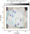 |
Fig. 1 Grayscale image of the noise in the polarized intensity map from the epoch 024 observations of ELAIS-N1 at 114.9–177.4 MHz. The pattern seen is due to the facet layout used in the DDF-pipeline. The angular resolution of the observations is 20′′. The green square shows the region chosen to test our stacking technique (1.4 deg × 1.7 deg). The cyan square represents the ELAIS-N1 field originally defined by Oliver et al. (2000). The larger orange square represents the area imaged by Grant et al. (2010) at 1.4 GHz. The red squares represent the locations of the detected polarized sources in the epoch 024 data alone. The blue circles represent the locations of the detected polarized sources after using the stacking technique for the six epochs described in the text. |
2.3 RM synthesis
In the simplest scenario, in which the background radiation is Faraday rotated due to a foreground magneto-ionic medium, the Faraday depth is equivalent to the RM (see e.g., Mao et al. 2014). Rotation measure synthesis (Brentjens & de Bruyn 2005) was performed on the Stokes Q and U data using pyrmsynth_lite8, a modified version of pyrmsynth9 intended to analyze the polarization cubes produced as part of the second data release of LoTSS, developed by one of us (S. Bourke). Polarized intensity images and RM cubes with a span in Faraday depth, ϕ, of ± 450 rad m−2 and a resolution of 0.3 rad m−2 were created. To avoid instrumental polarization, we excluded the range [ − 3, + 1.5] rad m−2. This range isasymmetric around zero rad m−2 because of corrections for ionospheric Faraday rotation as described in Sect. 2.2. RMCLEAN (Heald et al. 2009) was used after running the RM synthesis. Images in the Faraday depth range [350,450] radm−2, where no polarization signal is expected, were generated as a direct representation of the noise in our RM cubes, σQU. We used these noise maps to calculate our sensitivity.
The resolution in Faraday depth, δϕ, of our data is 0.9 rad m−2, the maximum observable Faraday depth, |ϕmax|, is 300 rad m−2, and the largest scale in ϕ space to which our data are sensitive is 1.07 rad m−2. These numbers were calculated using Eqs. (61)–(63) from Brentjens & de Bruyn (2005). Due to bandwidth depolarization, we lose sensitivity to large RM sources (at the low-frequency end). However, we do not expect this to be an issue for this field because the expected RM contribution from the Galaxy is low (<40 rad m−2; e.g., Oppermann et al. 2015).
Figure 2 shows the rotation measure spread function (RMSF) for the reference epoch (i.e., a single observation run) and the stacked data (of six observation runs; see Sect. 3 for details on the reference epoch and the stacking technique) of the ELAIS-N1 observations. The measured full width at half maximum (FWHM) of the RMSF is 0.9 rad m−2 (confirming the computed resolution in Faraday depth), and the increment in Faraday depth is 0.3 rad m−2. The noise of the stacked data is lower than that of the reference epoch.
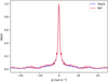 |
Fig. 2 Rotation measure spread function (RMSF) corresponding to the observations used in this paper. The data from the reference epoch alone are shown in red, and from the stacked data in blue (see text for more details). |
2.4 Source extraction
An in-depth analysis of the completeness and reliability of a comprehensive catalog of the polarized sources in the field is beyond the scope of this paper. This will be a matter for a follow-up paper. Instead we focus on the most reliably identified sources, using a detection threshold of 8σQU. This threshold is based on the results of George et al. (2012), who analyzed the false detection rates as a function of S/N and found the false detection rate to be less than 10-4 for an 8σQU detection threshold.
To identify the locations of polarized sources in the field, we divided the polarized intensity map by the noise map, both resulting from running RM synthesis, and derived a S/N map. We then searched the S/N map for pixels above the detection threshold. Each group of connected pixels (or island) was visually inspected in the polarized intensity map and identified in the Stokes I map to ensure a reliable detection. If only one isolated pixel was found above the threshold and/or no Stokes I counterpart was associated with an island, the detection was rejected. The Stokes I maps are presented inSabater et al. (2021).
We do not expect the instrumental polarization to be greater than 0.2%. Therefore, we calculated the observed fractional polarization, Π (defined as the ratio of the peak polarized intensity to the peak intensity in Stokes I, both at 20′′), and used this threshold to reject spurious polarized sources. We used the Stokes I map at 20′′ angular resolution (Sabater et al. 2021) to calculate this fraction. Six sources were removed from the final catalog of detected sources since they had a fractional polarization lower than 0.2%. One of these sources is shown as an example in Fig. 3. For this source, we find that the polarized intensity decreases substantially after the stacking procedure described in Sect. 3, consistent with the conclusion that it is artificially polarized. We present the catalog of detected polarized sources in Sect. 4.2.
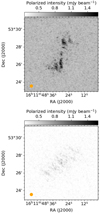 |
Fig. 3 Polarized intensity maps of a source rejected as spuriously polarized by the criterion of >0.2% fractional polarization, for the reference epoch (top) and stacked data (bottom). |
3 Stacking technique
Since we do not perform a full polarization calibration, possible changes in the polarization angle from different observing runs may be present. Taking into account that there is no absolute polarization angle calibration, we used a small region of the field (2.4 deg2, see Fig. 1) to test several approaches to the polarization angle alignment and stacking. This minimized the time needed to process the polarization data (to obviate the alternative of several weeks of computing time to process the full 16 deg2). We chose this region because it contains the strongest polarized source in the field (with a peak polarized intensity, Pp, of ~5 mJy beam−1) as well as a faint, potentially polarized source (with a S/N of ~7 in a single epoch).
The stacking technique presented here consists of the combination of the individual Stokes Q and U frequency channel images of each observed epoch. In other words, the data cube of each epoch is separated into the individual Q and U channel maps, and we stack each channel of each epoch together. For this, we used the toolkit for assembling Flexible Image Transport System (FITS) images into custom mosaics, Montage10 (Berriman et al. 2003). In our case, since all our epochs are centered at the same coordinates, we can use it to stack our data.
As noted above, due to ionospheric correction effects, the polarization angle may differ between separate epochs. Therefore, we need to align them before incoherently adding additional epoch data to avoid depolarizing the sources. To align the polarization angle, we used the 5 mJy beam−1 polarized source as the reference source (later labeled as source 02, see Sect. 4.2). We then calculated the reference polarized angle as the one corresponding to the coordinates of the peak pixel of the reference source in the polarized intensity image. These coordinates are RA = 241.4080 and Dec = 54.6551 (deg, J2000). The polarization angle, χ, is calculated from the Stokes Q and U:
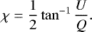 (1)
(1)
In order to choose the reference epoch, we plotted the polarization angle versus λ2 for each epoch (see Fig. 4). With this plot we can see a roughly constant angle offset between the observations, as expected. This plot can also be used to flag or down-weight those epochs showing a slope or scatter outside the range of the others. We chose epoch 024 as the reference epoch, as it was the one with the smallest uncertainty in its gradient and the greatest S/N in its polarized intensity image.
We attempted applying angle corrections using individual Q,U values per channel or, alternatively, the average angle difference across a broad range of frequencies (by calculating the slope of the polarization angle as a function of λ2 of one frequency subband), but these methods were not ideal. The main disadvantages are that the polarization angle correction is sensitive to channel-dependent noise and/or artifacts, and the shift in polarization angle depends on the frequency range chosen. Instead, we used a method based on the angles determined through the coherent addition of the signal across the full band using RM synthesis. However, future, more advanced correction techniques could also include a combination of several methods.
We calculated the polarization angles using the peak pixel of the reference source in the coherently band-averaged Stokes Q,U images following RM synthesis. This provides the polarization angle at the average wavelength-squared value,  . Since the number of flagged channels differs between the epochs, the value of
  is slightly different for different epochs. Therefore, in order to calculate the difference between the reference polarization angle and the one of the epoch to be corrected, first we have to calculate the angle of the latter at the reference
  . For this purpose, we used the RM value of the RM map output from RM synthesis at the same peak pixel. In this case, we ran RM synthesis for each epoch, using the range of ± 10 rad m−2 (the RM value is at ~6 rad m−2) with a sampling of 0.01 rad m−2 (i.e., higher than described in Sect. 2.3). This was done to achieve better Faraday depth sampling for a more precise correction, as we expect the RMs to be different by 0.1–0.3 rad m−2 after the ionospheric Faraday rotation correction (e.g., Sotomayor-Beltran et al. 2013). Table 1 shows the date at which the observation started (Sabater et al. 2021),
  values, and the RM measured at the peak pixel of the reference source and its uncertainty (calculated as the resolution in Faraday depth divided by twice the S/N of the detection, Brentjens & de Bruyn 2005) for each epoch.
We then calculated the polarization angle of the epoch to be corrected at the reference  ,
,  (where ep refers to the epoch to be corrected), as follows:
 (2)
(2)
where  is the polarization angle of the epoch to be corrected, calculated from the resulting Q and U maps after running RM synthesis on that epoch, RMep is the RM taken from the resulting RM map from RM synthesis of the epoch to be corrected,
  is the average wavelength-squared value of the reference epoch, and
  is the average wavelength-squared value of the epoch to be corrected.
Once we calculated the reference polarization angle and the angle of the epoch to be corrected, we applied the difference,
 (3)
(3)
to each pixel of each channel in Stokes Q and U using the following relations:
 (4)
(4)
 (5)
(5)
Here, Qcorr,ep and Ucorr,ep are the corrected Stokes Q and U channels and pep is the polarized intensity of the epoch to be corrected:
 (6)
(6)
The polarization angle corrections as applied to each epoch using this method, and their errors, are listed in Table 1. The errors in the polarization angle correction have been calculated following error propagation rules, where the errors in Q and U are the rms values of the resulting Q and U maps from RM synthesis, respectively.
Once the polarization angle corrections were applied to the data, we stacked the individual Q and U channels using Montage and ran RM synthesis on the stacked data with the parameters described in Sect. 2.3. Figure 5 shows the polarized intensity and the polarization angle versus frequency at the peak pixel of the reference source on the reference epoch and the stacked data. The decrease in noise of the polarized intensity and the reduced scatter in the polarization angle versus wavelength squared after stacking the data are noticeable. In addition, to check if an angle correction using a single source as reference works well for the entire field, we also plot in Fig. 5 the polarized intensity and the polarization angle versus frequency at the peak pixel of the source named later as 01 (see Sect. 4.2) on the reference epoch and the stacked data. We chose this source because it is the farthest from the reference source (source 02, see Fig. 1) with an angular separation of 3.46 deg. We can see the improvements on source 01 as well, demonstrating the validity of the stacking technique. We used this method to correct for the polarization angle on the entire field and stacked the Q,U images for the six epochs used in this work.
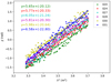 |
Fig. 4 Polarization angle, χ, versus observing wavelength squared, λ2, for a subset of the full frequency range for each of the individual epochs, overlaid in different colors. The equations for the lines of best fit for each epoch are also shown. |
Summary of observation date,  , RM of the reference source (using a higher sampling of Faraday depth, see text for details), and applied polarization position angle correction foreach observed epoch.
4 Results and discussion
4.1 Stacked data versus reference epoch
We computed the rms noise level (see Sect. 2.3) across the entire field (16 deg2), and we obtained a minimum of 63 μJy beam−1 for the reference epoch, σQU,ref, and a minimum of 26 μJy beam−1 for the stacked data (six epochs), σQU,stack. The median rms noise level across the entire field is 111 μJy beam−1 for the reference epoch ( ) and 44 μJy beam−1 for the stacked data (
 ). Therefore, the noise has been reduced by ~
  after stacking six epochs, as expected from Gaussian statistics.
Figure 6 shows the polarized intensity maps (not deconvolved) of the reference source and the source named later as 09 (see Sect. 4.2) before and after applying the stacking technique, respectively.This further verifies the stacking technique because fainter sources are successfully detected; for example, the latter source that would not have been detected in a single epoch using a detection threshold of 8σQU.
4.2 Catalog of polarized sources
Table 2 lists the properties of the detected polarized sources in the ELAIS-N1 field. Using the source extraction method described in Sect. 2.4, we detected ten polarized sources in our stacked data, seven of which were not detected in the reference epoch alone (using a detection threshold of 8σQU). Therefore, with our resolution and sensitivity, we detect one polarized source per 5.3 deg2 before stacking (in agreement with earlier estimates, e.g., Van Eck et al. 2018) and one polarized source per 1.6 deg2 after stacking our data. This value should be taken as a lower limit of the true low-frequency polarized source density at this sensitivity, considering that our catalog might be incomplete due to the high chosen detection threshold (see Sect. 2.4) and the exclusion of the RM range near 0 rad m−2.
The peak polarized intensity of the source (Cols. 5 and 6 of our catalog, see Table 2) is corrected for polarization bias following George et al. (2012). We used the rms at the peak pixel location of the source detection to calculate the S/N (Cols. 7 and 8 of our catalog). Columns 9 and 10 of our catalog show the RMs of the sources. The RM synthesis was run with the parameters described in Sect. 2.3. A parabola was fitted around the peak to improve the precision of the RM measurement. The error in the RM was calculated as the RM resolution divided by twice the S/N of the detection (Brentjens & de Bruyn 2005). We note that the RM measurements presented in Tables 1 and 2 for the reference source 02 differ because of the different RM synthesis parameters used for the polarized angle correction (see Sect. 3) and the default data processing (see Sect. 2.3).
As mentioned before, polarized radio source counts are important for studying the changes in the properties of radio source populations.However, the number of detected sources presented in this paper is very low, and therefore this analysis will be discussed in a follow-up paper based on deeper images.
The LOFAR images of the detected polarized sources and their Faraday spectra at the location of the peak polarized intensity, using the stacked data, are shown in Fig. 7. The Faraday spectra are zoomed in on to show the Faraday range containing the peak (only one Faraday depth component was found in all cases). We plotted the polarized intensity maps with the Stokes I contours overlaid, starting at 55 times the median rms noise level of the Stokes I map, σI, and increasing by factors of two for sources 01, 02, and 03 (to avoid showing artifacts); at 20σI and increasing by factors of two for sources 04, 06, 07, and 09; and at 10σI and increasing by factors of  for the remaining sources. The angular resolution of the Stokes I maps is 6′′, and 20′′ for the polarized intensity images. In addition, we overlaid horizontal lines on the Faraday spectra representing the 3σQU and 8σQU levels, using the derived σQU value at the location of the peak polarized intensity. We also highlight the area in Faraday depth excluded due to the instrumental polarization in gray. The locations of the detected sources in the sky are also shown in Fig. 1.
Table 3 shows the redshifts for nine of the ten detected polarized sources. Kondapally et al. (2021) cross-matched the PyBDSF11 radio catalog from total-intensity observations of Sabater et al. (2021) using various optical to infrared surveys. The LOFAR cross-identifications are used to then generate photometric redshifts and obtain existing spectroscopic redshifts as described by Duncan et al. (2021). Sources 01, 03, and 10 were outside of the multiwavelength surveys used for the radio cross-matching in Kondapally et al. (2021). Therefore, their counterparts were searched for using the NASA/IPAC Extragalactic Database (NED12). The redshift of the counterpart associated with source 04 was flagged as possible, but doubtful, by Kondapally et al. (2021). For this reason, NED was used to estimate the redshift of source 04 as well. Nevertheless, the host ID for this source should be considered as uncertain. The corresponding references found in NED are shown in Table 3. No counterpart for source 07 was found.
The redshifts of the polarized sources provide the prospect of converting the measured RMs to that in the sources’ rest frames (e.g., Michilli et al. 2018). This requires the RM contribution from the Galactic foreground to be subtracted prior to the redshift correction. Since the uncertainties in the Galactic RM (GRM) foreground are comparable to the precise RM measurements in this work (see Sect. 4.5, Table 7), we do not make this correction but note that this can be addressed in future work. Furthermore, this motivates the requirement for a denser and more accurate “RM Grid” to reconstruct the GRM foreground (e.g., Heald et al. 2020).
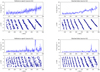 |
Fig. 5 Polarized intensity and polarization angle versus frequency at the peak pixel of the reference source (named source 02) on the reference epoch (upper left) and the stacked data (upper right), and at the peak pixel of source 01 on the reference epoch (bottom left) and the stacked data (bottom right). The prominent spikes in the plots are likely due to RFI-related issues, and the different impact on the different sources might be due to the facet-based calibration. |
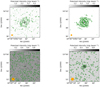 |
Fig. 6 Polarized intensity map (not deconvolved) of the reference source (named 02, see text for details) (top panels) and of the source named 09 (bottom panels) before (left) and after (right) applying the stacking technique. Green contours showing the polarized intensity start at 3σQU,ref
and increase by factors of |

4.3 Analysis of results from the individual epochs
Here, we analyze the Faraday spectra and the characteristics of detected polarized sources for each individual epoch. Figure 8 shows the Faraday spectrum of source 09 plotted for each observed epoch. The overlaid horizontal lines represent the 3σQU and 8σQU levels, usingthe median of the rms noise levels for each epoch. We can see that source 09 only satisfies the 8σQU detection threshold for some of the epochs, demonstrating that the stacking technique is important for detecting those sources that are very close to the detection threshold limit.
Table 4 lists the polarized intensity, Pp, the RM, and the S/N (as described in Sect. 4.2) for sources 02 and 09 measured at each epoch used here. The polarized intensity is given even if the S/N is below 8 (our detection threshold). It is also worth noting that the S/N does not behave in the same way for each epoch. As shown in Table 4, the epoch with the highest S/Ns for source 02 is not the same as the one for source 09.
The average polarized intensity for sources 02 and 09 over the six observing epochs is 4.84 and 0.84 mJy beam−1, respect- ively. However, the polarized intensity measured using the stack- ed data is 4.69 mJy beam−1 for source 02 and 0.80 mJy beam−1 for source 09. Therefore, the stacking technique seems to cause a small depolarization, which decreases the polarized intensity by ~4%. On the other hand, the decrease in polarized intensity is very small compared to the decrease in noise (~2.5 times lower), making the stacking technique a valuable tool to help detect fainter sources. Another source of the depolarization may be our inability to fully correct for the ionospheric Faraday rotation behavior over the observations. This approximate level of depolarization could be expected from residual RM errors (e.g., using Eq. (34) from Sokoloff et al. 1998).
Catalog of polarized sources in the ELAIS-N1 field detected with LOFAR at 146 MHz.
4.4 Measurements as a function of number of stacked epochs
Here, we analyze the effect of stacking a different number of epochs. We show source 09 as an example. Figure 9 and Table 5 show the evolution of the Faraday spectra by stacking a different number of epochs. The overlaid horizontal lines in Fig. 9 represent the 8σQU levels, using the median of the rms noise level of the corresponding number of stacked epochs. In Table 5, the column Nepoch corresponds to the number of epochs stacked. We list the polarized intensity also in the case where the S/N is below 8 (our detection threshold).
The S/N of the source increases continuously with the number of epochs stacked. A large improvement is seen when comparing one epoch to the stacking of two epochs (the median noise goes down by more than  ), which we believe is due to the presence of the instrumental polarization close to ϕ = 0. The instrumental polarization responses are uncorrelated between epochs, resulting in a larger than expected decrease in the noise.
Redshifts of the LOFAR-detected polarized sources.
4.5 Comparison with 1.4 GHz measurements
We cross-matched our catalog of detected polarized sources with the catalog of Grant et al. (2010), who found 136 polarized sources at 1.4 GHz in the ELAIS-N1 field. Their observations had an angular resolution of 42′′ × 62′′ (at the field center). We used a matching radius of 1.5′ (to include sources similar to our source 07) and found five matches. In Table 6, we give the name, the peak intensity in Stokes I at 146 MHz, Sp,146, the peak intensity in Stokes I at 1.4 GHz, Sp,1420, the spectral index, α1420-32513, the fractional polarization at 146 MHz, Π146, and the fractional polarization at 1.4 GHz, Π1420, of these five sources.
Figure 1 shows the overlapping area between our observations and the field imaged by Grant et al. (2010) at 1.4 GHz. Sources 01 and 03 are outside of the area covered by Grant et al. (2010). Therefore, we have 1.4 GHz measurements for five out of eight polarized sources.
In Fig. 7, we plot the locations of the polarized sources detected at 1.4 GHz by Taylor et al. (2007) and Grant et al. (2010) on our polarized intensity maps (when corresponding). We can see that the centroids from Grant et al. (2010), whose observations were more sensitive than the ones of Taylor et al. (2007), are more consistent with the LOFAR locations.
Taylor et al. (2009) derived RMs for several tens of thousands of polarized radio sources using NVSS data. We cross-matched our catalog with theirs using a matching radius of 1.5′ and found two counterparts. Table 7 shows the RM comparison between our data and the data from Taylor et al. (2009). The RM of source 01 is different at ~4σ. However, since this source is a blazar, variability might play a role (see e.g., Anderson et al. 2019). The RM of source 02 is consistent within ~1σ. The GRM values at the location of each source are also shown in Table 7. We obtained these values using the reconstruction of the Galactic Faraday depth sky from Hutschenreuter & Enßlin (2020)14. Eight of the LOFAR sources are consistent with each GRM value within ~1σ, indicating that the Milky Way RM dominates the mean RM (as expected). Sources 05 and 10 are the most different (~4σ and ~2.4σ, respectively).
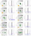 |
Fig. 7 Polarized intensity maps with overlaid Stokes I contours (green) and Faraday spectra of the LOFAR detected polarized sources. The orange and yellow circles in the bottom left corners represent the synthesized beam of the observations in polarization (20′′) and in Stokes I (6′′), respectively. The Stokes I contours start either at 55σI or 20σI and increase by factors of two, or at 10σI and increase by factors of |

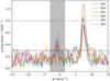 |
Fig. 8 Faraday spectra of source 09 for each epoch. The dashed and dotted black horizontal lines represent the 3σQU and 8σQU levels, respectively (see text for details). The vertical gray area represents the range around ϕ = 0 rad m−2 excluded from the analysis due to instrumental polarization. |
Measurements for sources 02 and 09 in each epoch.
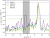 |
Fig. 9 Faraday spectra of source 09 for different numbers of stacked epochs. The dotted horizontal lines represent the corresponding 8σQU levels. The vertical gray area represents the range around ϕ = 0 rad m−2 excluded from the analysis due to instrumental polarization. |
Measurements for source 09 using different numbers of stacked epochs.
146 MHz and 1.4 GHz properties of the detected polarized sources.
RM comparison.
4.6 Morphology and polarized emission
By inspecting the 6′′ total-intensity images of our detected polarized sources (see Fig. 7), we identify three compact sources (sources 01, 03, and 04, classified as blazars in NED), three FR II radio galaxies (sources 06, 07, and 09), and three FR I radio galaxies (sources 05, 08, and 10). Source 02 seems to be a double-lobed radio galaxy. The number of FR I radio galaxies detected in polarization represents a much greater fraction of this type of object than seen in the first data release area of LoTSS (Van Eck et al. 2018 found one out of 92 detected polarized sources), which suggests that more sensitive observations may help with the detection of the polarized emission from extended regions of FR I radio galaxies (O’Sullivan et al. 2018). Sources 01, 03, and 04 have been classified as BL Lacertae objects by Healey et al. (2008), Abdo et al. (2010), and D’Abrusco et al. (2014), respectively. Future observations of these sources (and in particular of source 02) with the addition of the LOFAR international baselines (which could provide an angular resolution of 0.4′′ at 140 MHz, see Moldón et al. 2015) would reveal the source morphology in detail.
The FR I-type sources have the lowest mean redshift (0.1470), compared to the blazars (0.3733) and the FR II sources (0.7062). This is expected and consistent with the general trend in radio power for FR I versus FR II sources (see e.g., Mingo et al. 2019). However, the FR I-type sources have the largest absolute RMs (16.3 rad m−2), compared to the blazars (6.7 rad m−2) and the FR II sources (5.0 rad m−2). This may be reflecting the environment in which the polarized emission originates, for example the inner jet for FR I sources versus hotspots of FR II.
Some ofour detected polarized sources show polarization in their core or inner jets. Since the core of a radio galaxy is not expected to be strongly polarized (e.g., Saikia & Kulkarni 1998), this may represent polarized emission originating from the inner jets in a region of highly ordered magnetic field, or possibly indicate restarted radio galaxy activity (e.g., Mahatma et al. 2019).
In Fig. 7, we can also see that Grant et al. (2010) detect one of the lobes of source 07 at 1.4 GHz that is not detected using LOFAR at 146 MHz. This may be an example of the Laing-Garrington effect (Laing 1988; Garrington et al. 1988), which is based on the fact that depolarization with increasing wavelength is usually larger for the weaker flux density lobe (corresponding to the counter-jet farther from us). In principle, large numbers of detections of this effect can probe the properties of the environments of distant radio galaxies.
5 Summary
We used LOFAR to observe the ELAIS-N1 field at 146 MHz over several epochs and analyzed the resulting 20′′ -resolution polarimetric images. In order to achieve sensitivities not limited by the thermal noise of standard eight-hour LOFAR observations, a stacking technique was developed. The outcomes of this analysis are:
- 1.
We have demonstrated the feasibility of the stacking technique presented here. With this technique, we were able to reach a 1σQU rms noise level of 26 μJy beam−1 in the central part of the field. After stacking six epochs, the median noise across the field was reduced by
 in comparison to the reference epoch.
 - 2.
We detected ten polarized sources in the stacked data, using an 8σQU detection threshold. Seven of these sources were not detected in the reference epoch alone. We have presented radio images and RM measurements of the detected sources.
- 3.
Since the imaged area is of 16 deg2, the polarized source surface density is one per 1.6 deg2 at the resolution and sensitivity of our observations. This should be considered a lower limit of the true number density.
- 4.
We have detected a larger fraction of FR I radio galaxies (three out of ten) than in previous, less sensitive observations (e.g., one out of 92, Van Eck et al. 2018), which suggests that increasingly sensitive LOFAR observations may help to detect and characterize the magnetic field structure in this type of object at low frequencies.
This work provides a valuable tool for the study of deep observations in polarization at very low frequencies, and in particular for the initial analysis of the ELAIS-N1 field. The next steps will be to combine all of the available observations of the field (including new observations taken in recent cycles and further allocated observations of the field), to further decrease the detection threshold, to characterize the reliability and completeness of the catalog of detected sources, andto analyze the polarized source counts on the basis of an increased number of detected sources. In addition, the stacking technique presented here can also be applied to the other LoTSS Deep Fields (Lockman Hole and Boötes) in the future, as well as to the GOODS-N (Great Observatories Origins Deep Survey – North) field.
Acknowledgements
We thank the anonymous referee for the valuable and constructive comments, which have helped to improve thispaper. This paper is based on data obtained with the International LOFAR Telescope (ILT) under project codes LC0_019, LC2_024 and LC4_008. LOFAR (van Haarlem et al. 2013) is the Low Frequency Array designed and constructed by ASTRON. It has observing, data processing, and data storage facilities in several countries, that are owned by various parties (each with their own funding sources), and that are collectively operated by the ILT foundation under a joint scientific policy. The ILT resources have benefitted from the following recent major funding sources: CNRS-INSU, Observatoire de Paris and Université d’Orléans, France; BMBF, MIWF-NRW, MPG, Germany; Science Foundation Ireland (SFI), Department of Business, Enterprise and Innovation (DBEI), Ireland; NWO, The Netherlands; The Science and Technology Facilities Council, UK. N.H.R. acknowledges support from the BMBF through projects D-LOFAR IV (FKZ: 05A17PC1) and MeerKAT (FKZ: 05A17PC2). V.J. acknowledges support by the Croatian Science Foundation for the project IP-2018-01-2889 (LowFreqCRO). The authors of the Polish scientific institutions thank the Ministry of Science and Higher Education (MSHE), Poland for granting funds for the Polish contributionto the ILT (MSHE decision no. DIR/WK/2016/2017/05-1) and for maintenance of the LOFAR PL-610 Borowiec, LOFAR PL-611 Lazy, LOFAR PL-612 Baldy stations. J.S. is grateful for support from the UK STFC via grant ST/R000972/1. M.J.H. acknowledges support from the UK Science and Technology Facilities Council (ST/R000905/1). R.K. acknowledges support from the Science and Technology Facilities Council (STFC) through an STFC studentship via grant ST/R504737/1. P.N.B. is grateful for support from the UK STFC via grant ST/R000972/1. I.P. acknowledges support from INAF under the SKA/CTA PRIN “FORECaST” and the PRIN MAIN STREAM “SAuROS” projects. This research made use of Montage. It is funded by the National Science Foundation under Grant Number ACI-1440620, and was previously funded by the National Aeronautics and Space Administration’s Earth Science Technology Office, Computation Technologies Project, under Cooperative Agreement Number NCC5-626 between NASA and the California Institute of Technology. This research made use of Topcat (Taylor 2005), available at http://www.starlink.ac.uk/topcat/, APLpy, an open-source plotting package for Python hosted at http://aplpy.github.com, and Astropy, a community-developed core Python package for Astronomy (Astropy Collaboration 2013). This research made use of the NASA/IPAC Extragalactic Database (NED), which is operated by the Jet Propulsion Laboratory, California Institute of Technology, under contract with the National Aeronautics and Space Administration.
References
- Abdo, A. A., Ackermann, M., Ajello, M., et al. 2010, ApJ, 715, 429 [NASA ADS] [CrossRef] [Google Scholar]
- Aihara, H., Armstrong, R., Bickerton, S., et al. 2018, PASJ, 70, S8 [NASA ADS] [Google Scholar]
- Albareti, F. D., Allende Prieto, C., Almeida, A., et al. 2017, ApJS, 233, 25 [NASA ADS] [CrossRef] [Google Scholar]
- Anderson, C. S., Gaensler, B. M., Feain, I. J., & Franzen, T. M. O. 2015, ApJ, 815, 49 [NASA ADS] [CrossRef] [Google Scholar]
- Anderson, C. S., O’Sullivan, S. P., Heald, G. H., et al. 2019, MNRAS, 485, 3600 [Google Scholar]
- Astropy Collaboration, (Robitaille, T. P., et al.) 2013, A&A, 558, A33 [NASA ADS] [CrossRef] [EDP Sciences] [Google Scholar]
- Beck, R., & Wielebinski, R. 2013, Planets, Stars and Stellar Systems (Dordrecht: Springer Science+Business Media) 5, 641 [CrossRef] [Google Scholar]
- Becker, R. H., White, R. L., & Helfand, D. J. 1995, ApJ, 450, 559 [NASA ADS] [CrossRef] [Google Scholar]
- Bernardi, G., Greenhill, L. J., Mitchell, D. A., et al. 2013, ApJ, 771, 105 [NASA ADS] [CrossRef] [Google Scholar]
- Berriman, G. B., Good, J. C., Curkendall, D. W., et al. 2003, ASP Conf. Ser., 295, 343 [Google Scholar]
- Bonafede, A., Feretti, L., Murgia, M., et al. 2010, A&A, 513, A30 [NASA ADS] [CrossRef] [EDP Sciences] [Google Scholar]
- Brentjens, M. A., & de Bruyn, A. G. 2005, A&A, 441, 1217 [NASA ADS] [CrossRef] [EDP Sciences] [Google Scholar]
- Burn, B. J. 1966, MNRAS, 133, 67 [NASA ADS] [CrossRef] [Google Scholar]
- Chakraborty, A., Roy, N., Datta, A., et al. 2019, MNRAS, 490, 243 [Google Scholar]
- Condon, J. J., Cotton, W. D., Greisen, E. W., et al. 1998, AJ, 115, 1693 [NASA ADS] [CrossRef] [Google Scholar]
- Condon, J. J., Cotton, W. D., Fomalont, E. B., et al. 2012, ApJ, 758, 23 [NASA ADS] [CrossRef] [Google Scholar]
- D’Abrusco, R., Massaro, F., Paggi, A., et al. 2014, ApJS, 215, 14 [NASA ADS] [CrossRef] [Google Scholar]
- de Gasperin, F., Dijkema, T. J., Drabent, A., et al. 2019, A&A, 622, A5 [NASA ADS] [CrossRef] [EDP Sciences] [Google Scholar]
- Duncan, K. J., Kondapally, R., Brown, M. J. I., et al. 2021, A&A, 648, A4 (LoTSS SI) [EDP Sciences] [Google Scholar]
- Falco, E. E., Kochanek, C. S., & Muñoz, J. A. 1998, ApJ, 494, 47 [NASA ADS] [CrossRef] [Google Scholar]
- Farnes, J. S., Gaensler, B. M., & Carretti, E. 2014, ApJS, 212, 15 [NASA ADS] [CrossRef] [Google Scholar]
- Garrington, S. T., Leahy, J. P., Conway, R. G., & Laing, R. A. 1988, Nature, 331, 147 [NASA ADS] [CrossRef] [Google Scholar]
- George, S. J., Stil, J. M., & Keller, B. W. 2012, PASA, 29, 214 [NASA ADS] [CrossRef] [Google Scholar]
- Grant, J. K., Taylor, A. R., Stil, J. M., et al. 2010, ApJ, 714, 1689 [NASA ADS] [CrossRef] [Google Scholar]
- Hales, C. A., Norris, R. P., Gaensler, B. M., et al. 2014a, MNRAS, 441, 2555 [NASA ADS] [CrossRef] [Google Scholar]
- Hales, C. A., Norris, R. P., Gaensler, B. M., & Middelberg, E. 2014b, MNRAS, 440, 3113 [NASA ADS] [CrossRef] [Google Scholar]
- Han, J. L. 2017, ARA&A, 55, 111 [NASA ADS] [CrossRef] [Google Scholar]
- Hardcastle, M. J., Alexander, P., Pooley, G. G., & Riley, J. M. 1997, MNRAS, 288, 859 [NASA ADS] [CrossRef] [Google Scholar]
- Heald, G., Braun, R., & Edmonds, R. 2009, A&A, 503, 409 [NASA ADS] [CrossRef] [EDP Sciences] [Google Scholar]
- Heald, G., Mao, S., Vacca, V., et al. 2020, Galaxies, 8, 53 [Google Scholar]
- Healey, S. E., Romani, R. W., Cotter, G., et al. 2008, ApJS, 175, 97 [NASA ADS] [CrossRef] [Google Scholar]
- Hopkins, A. M., Afonso, J., Chan, B., et al. 2003, AJ, 125, 465 [NASA ADS] [CrossRef] [Google Scholar]
- Hurley-Walker, N., Callingham, J. R., Hancock, P. J., et al. 2017, MNRAS, 464, 1146 [NASA ADS] [CrossRef] [Google Scholar]
- Hutschenreuter, S., & Enßlin, T. A. 2020, A&A, 633, A150 [EDP Sciences] [Google Scholar]
- Intema, H. T., van der Tol, S., Cotton, W. D., et al. 2009, A&A, 501, 1185 [NASA ADS] [CrossRef] [EDP Sciences] [Google Scholar]
- Jelić, V., de Bruyn, A. G., Mevius, M., et al. 2014, A&A, 568, A101 [NASA ADS] [CrossRef] [EDP Sciences] [Google Scholar]
- Kessler, M. F., Steinz, J. A., Anderegg, M. E., et al. 1996, A&A, 500, 493 [Google Scholar]
- Kondapally, R., Best, P. N., Hardcastle, M. J., et al. 2021, A&A, 648, A3 (LoTSS SI) [EDP Sciences] [Google Scholar]
- Laing, R. A. 1988, Nature, 331, 149 [NASA ADS] [CrossRef] [Google Scholar]
- Laing, R. A., & Bridle, A. H. 2014, MNRAS, 437, 3405 [NASA ADS] [CrossRef] [Google Scholar]
- Lawrence, A., Warren, S. J., Almaini, O., et al. 2007, MNRAS, 379, 1599 [NASA ADS] [CrossRef] [MathSciNet] [Google Scholar]
- Lenc, E., Gaensler, B. M., Sun, X. H., et al. 2016, ApJ, 830, 38 [NASA ADS] [CrossRef] [Google Scholar]
- Lonsdale, C. J., Smith, H. E., Rowan-Robinson, M., et al. 2003, PASP, 115, 897 [NASA ADS] [CrossRef] [Google Scholar]
- Mahatma, V. H., Hardcastle, M. J., Williams, W. L., et al. 2019, A&A, 622, A13 [NASA ADS] [CrossRef] [EDP Sciences] [Google Scholar]
- Manners, J. C., Johnson, O., Almaini, O., et al. 2003, MNRAS, 343, 293 [NASA ADS] [CrossRef] [Google Scholar]
- Mao, S. A., Banfield, J., Gaensler, B., et al. 2014, ArXiv e-prints, [ArXiv:1401.1875] [Google Scholar]
- Martin, D. C., Fanson, J., Schiminovich, D., et al. 2005, ApJ, 619, L1 [Google Scholar]
- Mauduit, J. C., Lacy, M., Farrah, D., et al. 2012, PASP, 124, 714 [NASA ADS] [CrossRef] [Google Scholar]
- McMahon, R. G., Walton, N. A., Irwin, M. J., et al. 2001, New Astron. Rev., 45, 97 [NASA ADS] [CrossRef] [Google Scholar]
- Mevius, M. 2018, Astrophysics Source Code Library [record ascl:1806.024] [Google Scholar]
- Michilli, D., Seymour, A., Hessels, J. W. T., et al. 2018, Nature, 553, 182 [NASA ADS] [CrossRef] [Google Scholar]
- Mingo, B., Croston, J. H., Hardcastle, M. J., et al. 2019, MNRAS, 488, 2701 [NASA ADS] [CrossRef] [Google Scholar]
- Mohan, N., & Rafferty, D. 2015, Astrophysics Source Code Library [record ascl:1502.007] [Google Scholar]
- Moldón, J., Deller, A. T., Wucknitz, O., et al. 2015, A&A, 574, A73 [NASA ADS] [CrossRef] [EDP Sciences] [Google Scholar]
- Morrissey, P., Conrow, T., Barlow, T. A., et al. 2007, ApJS, 173, 682 [Google Scholar]
- Mulcahy, D. D., Horneffer, A., Beck, R., et al. 2014, A&A, 568, A74 [NASA ADS] [CrossRef] [EDP Sciences] [Google Scholar]
- Neld, A., Horellou, C., Mulcahy, D. D., et al. 2018, A&A, 617, A136 [NASA ADS] [CrossRef] [EDP Sciences] [Google Scholar]
- Ocran, E. F., Taylor, A. R., Vaccari, M., Ishwara-Chandra, C. H., & Prandoni, I. 2020, MNRAS, 491, 1127 [Google Scholar]
- Offringa, A. R., van de Gronde, J. J., & Roerdink, J. B. T. M. 2012, A&A, 539, A95 [NASA ADS] [CrossRef] [EDP Sciences] [Google Scholar]
- Oliver, S., Rowan-Robinson, M., Alexander, D. M., et al. 2000, MNRAS, 316, 749 [NASA ADS] [CrossRef] [Google Scholar]
- Oliver, S. J., Bock, J., Altieri, B., et al. 2012, MNRAS, 424, 1614 [Google Scholar]
- Oppermann, N., Junklewitz, H., Greiner, M., et al. 2015, A&A, 575, A118 [NASA ADS] [CrossRef] [EDP Sciences] [Google Scholar]
- O’Sullivan, S., Brüggen, M., Van Eck, C. L., et al. 2018, Galaxies, 6, 126 [NASA ADS] [CrossRef] [Google Scholar]
- O’Sullivan, S. P., Machalski, J., Van Eck, C. L., et al. 2019, A&A, 622, A16 [NASA ADS] [CrossRef] [EDP Sciences] [Google Scholar]
- O’Sullivan, S. P., Brüggen, M., Vazza, F., et al. 2020, MNRAS, 495, 2607 [NASA ADS] [CrossRef] [Google Scholar]
- Planck Collaboration VI. 2020, A&A, 641, A6 [NASA ADS] [CrossRef] [EDP Sciences] [Google Scholar]
- Rengelink, R. B., Tang, Y., de Bruyn, A. G., et al. 1997, A&AS, 124, 259 [NASA ADS] [CrossRef] [EDP Sciences] [Google Scholar]
- Richards, G. T., Myers, A. D., Gray, A. G., et al. 2009, ApJS, 180, 67 [NASA ADS] [CrossRef] [Google Scholar]
- Riseley, C. J., Lenc, E., Van Eck, C. L., et al. 2018, PASA, 35, 43 [Google Scholar]
- Riseley, C. J., Galvin, T. J., Sobey, C., et al. 2020, PASA, 37, e029 [Google Scholar]
- Sabater, J., Best, P. N., Tasse, C., et al. 2021, A&A, 648, A2 (LoTSS SI) [EDP Sciences] [Google Scholar]
- Saikia, D. J., & Kulkarni, A. R. 1998, MNRAS, 298, L45 [Google Scholar]
- Shimwell, T. W., Röttgering, H. J. A., Best, P. N., et al. 2017, A&A, 598, A104 [NASA ADS] [CrossRef] [EDP Sciences] [Google Scholar]
- Shimwell, T. W., Tasse, C., Hardcastle, M. J., et al. 2019, A&A, 622, A1 [NASA ADS] [CrossRef] [EDP Sciences] [Google Scholar]
- Sirothia, S. K., Dennefeld, M., Saikia, D. J., et al. 2009, ASP Conf. Ser., 407, 27 [Google Scholar]
- Smirnov, O. M., & Tasse, C. 2015, MNRAS, 449, 2668 [NASA ADS] [CrossRef] [Google Scholar]
- Smolčić, V., Delvecchio, I., Zamorani, G., et al. 2017, A&A, 602, A2 [NASA ADS] [CrossRef] [EDP Sciences] [Google Scholar]
- Sobey, C., Bilous, A. V., Grießmeier, J. M., et al. 2019, MNRAS, 484, 3646 [NASA ADS] [CrossRef] [Google Scholar]
- Sokoloff, D. D., Bykov, A. A., Shukurov, A., et al. 1998, MNRAS, 299, 189 [NASA ADS] [CrossRef] [Google Scholar]
- Sotomayor-Beltran, C., Sobey, C., Hessels, J. W. T., et al. 2013, A&A, 552, A58 [NASA ADS] [CrossRef] [EDP Sciences] [Google Scholar]
- Stil, J. M., Krause, M., Beck, R., & Taylor, A. R. 2009, ApJ, 693, 1392 [NASA ADS] [CrossRef] [Google Scholar]
- Tasse, C. 2014a, ArXiv e-prints, [arXiv:1410.8706] [Google Scholar]
- Tasse, C. 2014b, A&A, 566, A127 [NASA ADS] [CrossRef] [EDP Sciences] [Google Scholar]
- Tasse, C., Hugo, B., Mirmont, M., et al. 2018, A&A, 611, A87 [NASA ADS] [CrossRef] [EDP Sciences] [Google Scholar]
- Tasse, C., Shimwell, T., Hardcastle, M. J., et al. 2021, A&A, 648, A1 (LoTSS SI) [EDP Sciences] [Google Scholar]
- Taylor, M. B. 2005, ASP Conf. Ser., 347, 29 [Google Scholar]
- Taylor, A. R., Stil, J. M., Grant, J. K., et al. 2007, ApJ, 666, 201 [NASA ADS] [CrossRef] [Google Scholar]
- Taylor, A. R., Stil, J. M., & Sunstrum, C. 2009, ApJ, 702, 1230 [NASA ADS] [CrossRef] [Google Scholar]
- Tingay, S. J., Goeke, R., Bowman, J. D., et al. 2013, PASA, 30, e007 [Google Scholar]
- Vacca, V., Oppermann, N., Enßlin, T., et al. 2016, A&A, 591, A13 [NASA ADS] [CrossRef] [EDP Sciences] [Google Scholar]
- Van Eck, C. L., Brown, J. C., Stil, J. M., et al. 2011, ApJ, 728, 97 [NASA ADS] [CrossRef] [Google Scholar]
- Van Eck, C. L., Haverkorn, M., Alves, M. I. R., et al. 2018, A&A, 613, A58 [NASA ADS] [CrossRef] [EDP Sciences] [Google Scholar]
- van Haarlem, M. P., Wise, M. W., Gunst, A. W., et al. 2013, A&A, 556, A2 [NASA ADS] [CrossRef] [EDP Sciences] [Google Scholar]
- van Weeren, R. J., Williams, W. L., Hardcastle, M. J., et al. 2016, ApJS, 223, 2 [NASA ADS] [CrossRef] [Google Scholar]
- White, R. L., Becker, R. H., Helfand, D. J., & Gregg, M. D. 1997, ApJ, 475, 479 [NASA ADS] [CrossRef] [Google Scholar]
- Williams, W. L., van Weeren, R. J., Röttgering, H. J. A., et al. 2016, MNRAS, 460, 2385 [NASA ADS] [CrossRef] [Google Scholar]
Python Blob Detection and Source Finder (Mohan & Rafferty 2015); https://www.astron.nl/citt/pybdsf
S(ν) ∝ να.
All Tables
Summary of observation date, , RM of the reference source (using a higher sampling of Faraday depth, see text for details), and applied polarization position angle correction foreach observed epoch.
Catalog of polarized sources in the ELAIS-N1 field detected with LOFAR at 146 MHz.
All Figures
|
Fig. 1 Grayscale image of the noise in the polarized intensity map from the epoch 024 observations of ELAIS-N1 at 114.9–177.4 MHz. The pattern seen is due to the facet layout used in the DDF-pipeline. The angular resolution of the observations is 20′′. The green square shows the region chosen to test our stacking technique (1.4 deg × 1.7 deg). The cyan square represents the ELAIS-N1 field originally defined by Oliver et al. (2000). The larger orange square represents the area imaged by Grant et al. (2010) at 1.4 GHz. The red squares represent the locations of the detected polarized sources in the epoch 024 data alone. The blue circles represent the locations of the detected polarized sources after using the stacking technique for the six epochs described in the text. |
| In the text | |
|
Fig. 2 Rotation measure spread function (RMSF) corresponding to the observations used in this paper. The data from the reference epoch alone are shown in red, and from the stacked data in blue (see text for more details). |
| In the text | |
|
Fig. 3 Polarized intensity maps of a source rejected as spuriously polarized by the criterion of >0.2% fractional polarization, for the reference epoch (top) and stacked data (bottom). |
| In the text | |
|
Fig. 4 Polarization angle, χ, versus observing wavelength squared, λ2, for a subset of the full frequency range for each of the individual epochs, overlaid in different colors. The equations for the lines of best fit for each epoch are also shown. |
| In the text | |
|
Fig. 5 Polarized intensity and polarization angle versus frequency at the peak pixel of the reference source (named source 02) on the reference epoch (upper left) and the stacked data (upper right), and at the peak pixel of source 01 on the reference epoch (bottom left) and the stacked data (bottom right). The prominent spikes in the plots are likely due to RFI-related issues, and the different impact on the different sources might be due to the facet-based calibration. |
| In the text | |
|
Fig. 6 Polarized intensity map (not deconvolved) of the reference source (named 02, see text for details) (top panels) and of the source named 09 (bottom panels) before (left) and after (right) applying the stacking technique. Green contours showing the polarized intensity start at 3σQU,ref
and increase by factors of |
| In the text | |
|
Fig. 7 Polarized intensity maps with overlaid Stokes I contours (green) and Faraday spectra of the LOFAR detected polarized sources. The orange and yellow circles in the bottom left corners represent the synthesized beam of the observations in polarization (20′′) and in Stokes I (6′′), respectively. The Stokes I contours start either at 55σI or 20σI and increase by factors of two, or at 10σI and increase by factors of |
| In the text | |
|
Fig. 8 Faraday spectra of source 09 for each epoch. The dashed and dotted black horizontal lines represent the 3σQU and 8σQU levels, respectively (see text for details). The vertical gray area represents the range around ϕ = 0 rad m−2 excluded from the analysis due to instrumental polarization. |
| In the text | |
|
Fig. 9 Faraday spectra of source 09 for different numbers of stacked epochs. The dotted horizontal lines represent the corresponding 8σQU levels. The vertical gray area represents the range around ϕ = 0 rad m−2 excluded from the analysis due to instrumental polarization. |
| In the text | |
Current usage metrics show cumulative count of Article Views (full-text article views including HTML views, PDF and ePub downloads, according to the available data) and Abstracts Views on Vision4Press platform.
Data correspond to usage on the plateform after 2015. The current usage metrics is available 48-96 hours after online publication and is updated daily on week days.
Initial download of the metrics may take a while.