© GRAVITY Collaboration 2021

1. Introduction

The distance to the Galactic Center (GC), R₀, can be measured directly from stellar orbits around Sgr A*, the radio source associated with the GC massive black hole (MBH) (see, e.g., Genzel et al. 2010 and Bland-Hawthorn & Gerhard 2016 for a recent overview of alternative methods). To this end, the stellar proper motion, given in angle per unit time, is compared to its radial velocity, obtained in absolute length per unit time from spectroscopic observations. The GC distance then directly follows as a scaling parameter between the two measurements. Best suited for measuring R₀ is S2, a massive young main-sequence B star on a 16-year orbit with a semimajor axis of a ≃ 125 mas and an apparent K-band magnitude m_k ≃ 14 (Ghez et al. 2003; Eisenhauer et al. 2005; Martins et al. 2008; Gillessen et al. 2009a, 2017; Habibi et al. 2017). During its pericenter passage in 2018, S2 was closely monitored in astrometry and spectroscopy (Gravity Collaboration 2018; Do et al. 2019). In particular, the GRAVITY instrument (Gravity Collaboration 2017) directly measured the distance between S2 and Sgr A* during the flyby at a high angular resolution of around 30 μas. The combination of ultra-high astrometric precision from near-infrared interferometry and the spectroscopic precision of ≲10 km s⁻¹ allowed us to determine the GC distance at the unprecedented precision of < 1% (Gravity Collaboration 2019).

Operating in the K-band, GRAVITY combines the light from either the four Unit Telescopes (UTs) or Auxiliary Telescopes (AT) of the ESO Very Large Telescope Interferometer (VLTI). Fringe-tracking on a bright reference object enables minute-long integration times on the fainter science target and measuring differential complex visibilities. The extremely high angular resolution of ≃3 mas results in very accurate astrometry with error bars between 10 μas and 100 μas (Gravity Collaboration 2017). However, the latest R₀ measurement in Gravity Collaboration (2020) indicates a possible systematic difference with earlier determinations (Gravity Collaboration 2018, 2019). While the shift is small, of only 𝒪(1%), it is nevertheless significant because of the high precision of the measurement.

The difference in the measured GC distance coincides with a change in the observing mode. GRAVITY observes the GC with two different methods, depending on the separation between Sgr A* and S2. Close to pericenter passage, that is, in 2017 and 2018, the sources were detected simultaneously in a single fiber pointing in the so-called single-beam mode. In later epochs, their separation exceeded the fiber field of view (FOV), and S2 and Sgr A* were targeted individually. This is referred to as dual-beam mode.

In single-beam mode, it is not possible to align the two sources with the fiber center. To further improve the GRAVITY astrometry, we therefore conducted an analysis of how optical aberrations affect the visibility measurement across the full FOV. A similar concept of field-dependent errors already exists in radio interferometry, where it is known as direction-dependent effects (DDEs; see, e.g., Bhatnagar et al. 2008; Smirnov 2011; Smirnov & Tasse 2015; Tasse et al. 2018 and references therein). The DDEs can arise either at the instrument level from the antenna beam pattern or at the atmospheric level, for example, from the ionosphere. In particular for the latest generation of interferometers (e.g. VLA, MeerKAT, and LOFAR¹) with a wide FOV and a large fractional bandwidth, DDEs cannot be neglected. However, to our knowledge, there is no equivalent discussion in the context of optical/near-IR interferometry.

Our analysis indeed shows that small optical imperfections in the beam combiner induce field-dependent phase errors that are reflected in the inferred binary separation. We developed an analytical model to describe this effect, and verified it by application to a dedicated test-case observation. When it is applied to the GC observations, the model induces a shift in the S2 relative position of about 0.1−0.2 mas in 2018 and ∼0.5 mas in 2017 in both right ascension (RA) and declination (Dec). Despite being small, the change is non-negligible at the high astrometric accuracy achieved by GRAVITY. We can show that the corrected 2017 and 2018 data agree with the dual-beam observations of 2019 and 2020. Furthermore, when the correction is retroactively applied to the data sets used in Gravity Collaboration (2018, 2019), the ensuing GC distance is fully consistent with the latest result (Gravity Collaboration 2020).

We introduce the analytical model in Sect. 2 and compare it to calibration measurements in Sect. 3. Verification from the binary test case and the improved S2 position are presented in Sect. 4, and we discuss the implications for the GC distance in Sect. 5. Finally, we conclude in Sect. 6.

2. Formal description of static aberrations and their effect on visibility measurements

Static aberrations along the optical path of the instrument affect the measured visibilities by introducing a complex field-dependent factor for each telescope. We express this gain in its polar representation and decompose it into a phase map ϕ_i(α) and an amplitude map A_i(α). Here, the index i labels the telescope, and α denotes positions in the image plane. Phase- and amplitude-maps lead to a modification of the observed complex visibilities V^obs from the well-known van Cittert-Zernike theorem (cf. Eq. (23)). As we demonstrate in the following, they are given by

$$\begin{array}{c}\hfill V^{\mathrm{obs}}=\frac{\int \mathrm{d}\mathit{\alpha }{A}_i\left(\mathit{\alpha }\right)A_j\left(\mathit{\alpha }\right)O\left(\mathit{\alpha }\right)e^{-2\pi i\mathit{\alpha }·{\mathit{b}}_{i,j}/\lambda +i({\varphi }_i\left(\mathit{\alpha }\right)-{\varphi }_j\left(\mathit{\alpha }\right))}}{\sqrt{\int \mathrm{d}\mathit{\alpha }{A}_i^2\left(\mathit{\alpha }\right)O\left(\mathit{\alpha }\right)\int \mathrm{d}\mathit{\alpha }{A}_j^2\left(\mathit{\alpha }\right)O\left(\mathit{\alpha }\right)}},\end{array}$$(1)

where b_i, j is the baseline vector between the two telescopes, and O(α) denotes the intensity distribution of the observed astronomical object.

In this section, we show that the phase- and amplitude-maps follow from optical aberrations. To this end, we start from the overlap integral, which determines the electromagnetic field from a single telescope arriving at the beam combiner. Subsequently, we propagate the effect of static aberrations from the overlap integral to the measured complex visibility to arrive at a rigorous derivation of Eq. (1). Finally, we account for the superposition of static and turbulent aberrations to obtain a formalism that is applicable in realistic observation scenarios.

2.1. Static field-dependent aberrations at fiber injection

Single-mode fibers transport the light collected by each telescope E_tel to the beam-combiner instrument. The overlap integral between light and the fiber mode E_fib then determines the transmitted electric field (Neumann 1988),

$$\begin{array}{c}\hfill E\left(\mathit{\beta }\right)=E_{\mathrm{fib}}\left(\mathit{\beta }\right)\times \eta =E_{\mathrm{fib}}\times {\displaystyle \int }\mathrm{d}\mathit{\xi }{E}_{\mathrm{tel}}\left(\mathit{\xi }\right)E_{\mathrm{fib}}^{\ast }\left(\mathit{\xi }\right).\end{array}$$(2)

We assumed a normalized fiber mode ∫dξ|E_fib(ξ)|² = 1 and expressed image-plane positions by two-dimensional vectors, ξ and β. Following the description of Perrin & Woillez (2019), the overlap integral was converted into the pupil plane by the Parseval-Plancharel theorem,

$$\begin{array}{c}\hfill \eta ={\displaystyle \int }\mathrm{d}\mathit{u}{\mathcal{F}}^{-1}\left[E_{\mathrm{obj}}\right]P\left(\mathit{u}\right){\mathcal{F}}^{-1}\left[E_{\mathrm{fib}}^{\ast }\right]\left(\mathit{u}\right),\end{array}$$(3)

where ℱ⁻¹ denotes the inverse Fourier transform, that is, transformation from the image to the pupil plane, and E_obj is the light emitted by the astronomical object. The latter is connected to ℱ⁻¹(E_tel) by multiplication with the pupil function P(u), corresponding to a convolution in the image plane. In the most simple case of a single point source located at α₀, the light is described by a pure phase ${\mathcal{F}}^{-1}[E_{\text{obj}}^{ps}]=\exp \left(-2\pi i\mathit{u}\cdot {\mathit{\alpha }}_0\right)$. The pupil- and image-plane coordinates, ξ and u, respectively, are Fourier-conjugate to each other and chosen to be dimensionless. That is, any length scale in the pupil plane is given by λu, where λ refers to the wavelength and u = |u|. To discuss our results, we converted the dimensionless image plane coordinates ξ into the corresponding angular separation in UT observations. In an aberration-free scenario, the pupil function of a spherical telescope with diameter 2r_tel and central obscuration 2r_cent simply is

$$\begin{array}{c}\hfill \stackrel{\sim }{P}\left(\mathit{u}\right)=\{\begin{array}{cc}0\hfill & \mathrm{if}u⩽r_{\mathrm{cent}}/\lambda \hfill \\ 1\hfill & \mathrm{if}{r}_{\mathrm{cent}}<u⩽r_{\mathrm{tel}}/\lambda \hfill \\ 0\hfill & \mathrm{if}u>r_{\mathrm{tel}}/\lambda \hfill \end{array}.\end{array}$$(4)

Optical aberrations multiply the pupil function by a position-dependent complex phase, and we considered the case of purely static aberrations. These are characterized by an optical path difference (OPD) d_pup(u) in the pupil plane that can be expanded in terms of Zernike polynomials $Z_n^m$,

$$\begin{array}{c}\hfill d_{\mathrm{pup}}\left(\mathit{u}\right)={\displaystyle \sum _{n=0}^{n_{\max }}\sum _{m=-n}^n{A}_n^m{Z}_n^m(\lambda \mathit{u}/r_{\mathrm{tel}}).}\end{array}$$(5)

We adopted the convention that $Z_n^m$ is dimensionless and the coefficient $A_n^m$ corresponds to the root mean square of the term over the unit circle. When the turbulence-free complex fiber mode apodized by the pupil function is defined as

$$\begin{array}{c}\hfill {\mathrm{\Pi }}_{⊚}=e^{2\pi i{d}_{\mathrm{pup}}\left(\mathit{u}\right)/\lambda }\stackrel{\sim }{P}\left(\mathit{u}\right){\mathcal{F}}^{-1}\left[E_{\mathrm{fib}}^{\ast }\right]\left(\mathit{u}\right),\end{array}$$(6)

the overlap integral reads

$$\begin{array}{c}\hfill \eta ={\displaystyle \int }\mathrm{d}\mathit{u}{\mathcal{F}}^{-1}\left[E_{\mathrm{obj}}\right]\left(\mathit{u}\right){\mathrm{\Pi }}_{⊚}\left(\mathit{u}\right).\end{array}$$(7)

The overlap integral obviously depends on the fiber profile, which for a perfectly aligned ideal single-mode fiber is

$$\begin{array}{c}\hfill {\mathcal{F}}^{-1}\left[{\stackrel{\sim }{E}}_{\mathrm{fib}}^{\ast }\right]=exp(-\frac{{\lambda }^2{u}^2}{2{\sigma }_{\mathrm{fib}}^2}).\end{array}$$(8)

GRAVITY was designed for optimal fiber injection (Pfuhl et al. 2014), which is obtained for ${\sigma }_{\text{fib}}=2r_{\text{tel}}\sqrt{2ln2}/\left(\pi ϵ\right)$ (Wallner et al. 2002). Here, the parameter ϵ is of order unity and describes the pupil shape.

From the comparison of the model predictions and the calibration measurements in Sect. 3.2, we find that pupil-plane distortions alone are not sufficient to describe the observed aberration pattern. We also need to account for optical errors in the focal plane. Misalignment of the optical fiber as well as higher order aberrations at fiber injection introduce a complex phase in Eq. (8) and can distort the amplitude of the fiber profile.

To illustrate the effect of focal plane aberrations, we can consider the three types of misalignment depicted in Fig. 1: (A) Lateral misplacement of the fiber by (δx,δy), which in the pupil plane produces a phase slope ξ_fib = (δx/f, δy/f), where f is the focal length. (B) Fiber tilt by an angle φ_fib = (φ₁, φ₂) with respect to the optical axis of the system, which shifts the back-propagated fiber mode by u_fib = φ ⋅ f/λ. Finally (C), a defocus or axial fiber misplacement by δz that introduces an additional phase curvature exp[π iδzλ/f² u²]. When all three effects are taken into account, the generalized fiber profile, projected onto the pupil, is (Wallner et al. 2002)

$$\begin{array}{cc}\hfill {\mathcal{F}}^{-1}\left[E_{\mathrm{fib}}^{\ast }\right]& ={\mathcal{F}}^{-1}\left[{\stackrel{\sim }{E}}_{\mathrm{fib}}^{\ast }\right](\mathit{u}-{\mathit{u}}_{\mathrm{fib}})\hfill \\ \hfill & \times exp\{-2\pi i[\frac{\pi \delta z}{2f^2}{(\mathit{u}-{\mathit{u}}_{\mathrm{fib}})}^2-{\mathit{\xi }}_{\mathrm{fib}}·(\mathit{u}-{\mathit{u}}_{\mathrm{fib}})]\}.\hfill \end{array}$$(9)

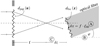Fig. 1. Schematic depiction of the pupil and focal plane aberrations that enter the overlap integral. Both effects in combination are required to describe the aberration patterns observed in calibration measurements. The lowest order aberrations in the pupil function are shown explicitly, which are (A) lateral fiber misplacement, (B) fiber tilt, and (C) defocus. Their effect is further explained in the text.

By rearranging the phase term in the pupil plane, we can decompose it into a piston, tip-tilt, and defocus

$$\begin{array}{cc}\hfill d_{\mathrm{fib}}^{\mathrm{piston}}\left(\mathit{u}\right)& =-\lambda (\frac{\delta z\lambda }{f^2}{\mathit{u}}_{\mathrm{fib}}+{\mathit{\xi }}_{\mathrm{fib}})·{\mathit{u}}_{\mathrm{fib}}-\frac{\delta z}{4f^2},\hfill \end{array}$$(10)

$$\begin{array}{cc}\hfill d_{\mathrm{fib}}^{\mathrm{tip}-\mathrm{tilt}}\left(\mathit{u}\right)& =\lambda (\frac{\delta z\lambda }{f^2}{\mathit{u}}_{\mathrm{fib}}+{\mathit{\xi }}_{\mathrm{fib}})·\mathit{u},\hfill \end{array}$$(11)

$$\begin{array}{cc}\hfill d_{\mathrm{fib}}^{\mathrm{defocus}}\left(\mathit{u}\right)& =-\frac{\delta z}{4f^2}(2{\lambda }^2{\mathit{u}}^2-1).\hfill \end{array}$$(12)

The phase terms in Eqs. (10)–(12) thus affect the overlap integral in the same way as the lowest order aberrations in d_pup(u). For the coordinate shift of the Gaussian profile, on the other hand, there is no such correspondence, and it alters the way in which the optical fiber scans the pupil-plane aberrations.

During GRAVITY observations, the misplacement term (A) depends on the performance of the fiber tracker, but also on the uncertainty of the source position. In particular for exoplanet observations, the latter can be sizable. Fiber tilt (B) is controlled by the GRAVITY pupil tracker, and the adaptive optics calibration is one example that affects the defocus (C).

While lateral misplacement (A) and defocus (C) describe the misplacement of a point-like fiber entrance, fiber tilt (B) accounts for the alignment of the fiber surface. This surface can exhibit irregularities beyond a simple tilt, which lead to a position-dependent OPD in the focal plane, d_foc(x), as illustrated in Fig. 1. Generally, aberrations from optical elements not conjugated to the pupil are field-dependent and known as Seidel aberrations. In this context, d_foc(x) arising in the focal plane constitutes an extreme example. It is still possible to decompose the focal plane distortions into a series of Zernike polynomials, in analogy to Eq. (5). In this representation, axial fiber offset (C) and fiber tilt (B) simply correspond to the lowest order coefficients, and higher order terms amount to a generalization of Wallner et al. (2002). Again, the phase terms introduced in ${\mathcal{F}}^{-1}\left[{\stackrel{\sim }{E}}_{\text{fib}}^{\ast }\right]$ by higher order aberrations are degenerate with d_pup(u), but the amplitude distortions need to be modeled explicitly by themselves.

Finally, for a single point source located at α₀ in the image plane, the overlap integral averaged over a timescale much longer than the source coherence time ⟨...⟩_obj is

$$\begin{array}{c}\hfill {\langle {\eta }^{\mathit{ps}}\rangle }_{\mathrm{obj}}\propto {\displaystyle \int }\mathrm{d}\mathit{u}{e}^{-2\pi i\mathit{u}·{\mathit{\alpha }}_0}{\mathrm{\Pi }}_{⊚}\left(\mathit{u}\right)=\mathcal{F}\left[{\mathrm{\Pi }}_{⊚}\right]\left({\mathit{\alpha }}_0\right).\end{array}$$(13)

Evaluation of the Fourier transform as a function of α₀ results in a two-dimensional complex map. We show several examples of such maps in Fig. 2, assuming different Zernike coefficients to determine d_pup(u). The perfect Airy pattern, obtained in the limit of zero aberrations, exhibits zero phase in the central part and a phase jump by 180° at |α| ≃ 1.22 λ/(2r_tel). Antisymmetric terms, such as tilt, coma, and trefoil (not shown), only alter the location and shape of the phase jump, while defocus (not shown), astigmatism, and higher order terms produce smooth phase gradients. For a general choice of d_pup(u) and in the absence of focal-plane aberrations, there is a saddle point where the phase maps average to zero, but significant phase shifts are encountered at larger radii.

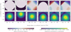Fig. 2. Example phase screens (top) and amplitude maps (bottom) in the image plane induced by low-order Zernike aberrations in the pupil plane at a wavelength of λ0 = 2.2 μm. From left to right: the considered aberrations are a perfect Airy pattern, a vertical tilt of 0.4 μm RMS, a vertical astigmatism of 0.2 μm RMS, a vertical coma of 0.2 μm RMS, and a combination of astigmatism, coma, and trefoil (with RMS 0.2 μm, 0.2 μm, and 0.1 μm, respectively). The rightmost panel also considers an additional fiber tilt with 0.2 μm RMS.

Focal-plane aberrations break the radial symmetry of the fiber profile. If the perturbations are small enough, however, the phase maps show a saddle point, but its value differs from zero and its location may be shifted. In any case, the transmitted amplitude is deformed and/or misplaced from the perfect Airy case. Pupil-plane aberrations typically widen the amplitude, while image-plane aberrations have the opposite effect. They lead to a widening of the fiber in the pupil plane, and correspondingly, to a narrower image-plane profile. The exact scaling relation for the position of the Airy ring remains true only approximately in the presence of higher order aberrations such that maps at two different wavelengths, λ₁ and λ₂, can be related by

$$\begin{array}{c}\hfill {\langle {\eta }^{\mathit{ps}}\rangle }_{\mathrm{obj}}({\alpha }_0,{\lambda }_1)\simeq {\langle {\eta }^{\mathit{ps}}\rangle }_{\mathrm{obj}}({\alpha }_0\frac{{\lambda }_2}{{\lambda }_1},{\lambda }_2).\end{array}$$(14)

2.2. Effect on visibility measurements and astrometry

The overlap integral defines the electromagnetic wave transmitted to the beam combiner from each of the four telescopes. After pairwise beam combination, the complex visibilities are obtained from the inference pattern I_i, j,

$$\begin{array}{cc}\hfill I_{i,j}& ={\displaystyle \int }\mathrm{d}\mathit{\beta }{\langle {|E_i\left(\mathit{\beta }\right)+E_j\left(\mathit{\beta }\right)|}^2\rangle }_{\mathrm{obj}}\hfill \end{array}$$(15)

$$\begin{array}{cc}& ={\langle {\left|{\eta }_i\right|}^2\rangle }_{\mathrm{obj}}+{\langle {\left|{\eta }_j\right|}^2\rangle }_{\mathrm{obj}}+2\mathfrak{R}{\langle {\eta }_i{\eta }_j^{\ast }\rangle }_{\mathrm{obj}},\hfill \end{array}$$(16)

where i and j denote the telescopes involved in the measurement, and I is the intensity. The complex pupil function enters each of these terms. Focusing on the single-telescope component first, we find from Eq. (7)

$$\begin{array}{cc}\hfill {\langle {\left|{\eta }_i\right|}^2\rangle }_{\mathrm{obj}}& ={\displaystyle \int }\mathrm{d}\mathit{\alpha }\mathcal{F}[{\mathrm{\Pi }}_{⊚,i}\otimes {\mathrm{\Pi }}_{⊚,i}]\left(\mathit{\alpha }\right)O\left(\mathit{\alpha }\right)\hfill \\ \hfill & ={\displaystyle \int }\mathrm{d}\mathit{\alpha }{\left|\mathcal{F}\left[{\mathrm{\Pi }}_{⊚,i}\right]\left(\mathit{\alpha }\right)\right|}^{2}O\left(\mathit{\alpha }\right),\hfill \end{array}$$(17)

where the ⊗-operator denotes autocorrelation, and O(α) = |E_obj(α)|² is the brightness distribution of the observed astronomical object, which obeys

$$\begin{array}{c}\hfill {\langle {\mathcal{F}}^{-1}\left[E_{\mathrm{obj}}\right]\left(\mathit{u}\right){\mathcal{F}}^{-1}{\left[E_{\mathrm{obj}}\right]}^{\ast }\left(\mathit{v}\right)\rangle }_{\mathrm{obj}}={\mathcal{F}}^{-1}\left[O\left(\mathit{\alpha }\right)\right](\mathit{u}-\mathit{v}).\end{array}$$(18)

Similarly, the inference term is given by

$$\begin{array}{cc}\hfill {\langle {\eta }_i{\eta }_j^{\ast }\rangle }_{\mathrm{obj}}& ={\displaystyle \int }\mathrm{d}\mathit{\alpha }\mathcal{F}[{\mathrm{\Pi }}_{⊚,i}\otimes {\mathrm{\Pi }}_{⊚,j}]\left(\mathit{\alpha }\right)O\left(\mathit{\alpha }\right)e^{-2\pi i\alpha ·{\mathit{b}}_{i,j}/\lambda }\hfill \\ \hfill & ={\displaystyle \int }\mathrm{d}\mathit{\alpha }\mathcal{F}\left[{\mathrm{\Pi }}_{⊚,i}\right]\left(\mathit{\alpha }\right)\mathcal{F}{\left[{\mathrm{\Pi }}_{⊚,j}\right]}^{\ast }\left(\mathit{\alpha }\right)O\left(\mathit{\alpha }\right)e^{-2\pi i\alpha ·{\mathit{b}}_{i,j}/\lambda },\hfill \end{array}$$(19)

where b_i, j is the baseline vector.

All optical aberrations discussed previously are encoded in the back-projected apodized pupil, which is a complex field-dependent function. Expressing the pupil function in its polar representation,

$$\begin{array}{c}\hfill \mathcal{F}\left[{\mathrm{\Pi }}_{⊚,i}\right]=A_i\left(\mathit{\alpha }\right)e^{i{\varphi }_i\left(\mathit{\alpha }\right)},\end{array}$$(20)

we refer to A_i as the telescope-dependent amplitude map and to ϕ_i as the phase map. These quantities are closely related to the photometric and the interferometric lobes, $L_i\left(\mathit{\alpha }\right)=A_i^2\left(\mathit{\alpha }\right)$ and

$$\begin{array}{c}\hfill L_{\mathrm{i},\mathrm{j}}\left(\mathit{\alpha }\right)=A_{\mathrm{i}}\left(\mathit{\alpha }\right)e^{i{\varphi }_{\mathrm{i}}\left(\mathit{\alpha }\right)}{A}_{\mathrm{j}}\left(\mathit{\alpha }\right)e^{-i{\varphi }_{\mathrm{j}}\left(\mathit{\alpha }\right)},\end{array}$$(21)

respectively.

From the measured inference pattern, the complex visibilities are obtained as

$$\begin{array}{c}\hfill V^{\mathrm{obs}}({\mathit{b}}_{i,j}/\lambda )={\langle {\eta }_i{\eta }_j^{\ast }\rangle }_{\mathrm{obj}}/\sqrt{{\langle {\left|{\eta }_i\right|}^2\rangle }_{\mathrm{obj}}{\langle {\left|{\eta }_j\right|}^2\rangle }_{\mathrm{obj}}}.\end{array}$$(22)

By contrast, in an ideal aberration-free setting, the van-Cittert-Zernike theorem relates the complex visibilities to the object brightness distribution

$$\begin{array}{c}\hfill V^{\mathrm{mod}}({\mathit{b}}_{i,j}/\lambda )=\frac{\int \mathrm{d}\mathit{\alpha }O\left(\mathit{\alpha }\right)e^{-2\pi i\alpha ·{\mathit{b}}_{i,j}/\lambda }}{\int \mathrm{d}\mathit{\alpha }O\left(\mathit{\alpha }\right)}·\end{array}$$(23)

Comparison of Eqs. (22) and (23) readily suggests that static aberrations at fiber injection distort both the measured visibility phases and amplitudes. We therefore need to adapt the interferometric equation accordingly. To make this effect even more explicit, we first considered the case of a single unresolved object at position α₀,

$$\begin{array}{c}\hfill V_{\mathit{ps}}^{\mathrm{obs}}({\mathit{b}}_{i,j}/\lambda )=\frac{L_{i,j}\left({\mathit{\alpha }}_0\right)}{\sqrt{L_i\left({\mathit{\alpha }}_0\right)L_j\left({\mathit{\alpha }}_0\right)}}{e}^{-2\pi i{\mathit{\alpha }}_0·{\mathit{b}}_{i,j}/\lambda }.\end{array}$$(24)

In the aberration-free case, the phase- and amplitude-maps of either telescope are given by the perfect Airy pattern, shown in the leftmost panel of Fig. 2, and ϕ_i/j(α₀) equals zero or 2π. The presence of static aberrations introduces a phase shift by ϕ_i(α₀) − ϕ_j(α₀). For an interferometric binary with positions α₁, α₂ and flux ratio f^bin, the measured visibility becomes

$$\begin{array}{c}\hfill V_{\mathrm{bin}}^{\mathrm{obs}}=\frac{L_{i,j}\left({\mathit{\alpha }}_1\right)e^{-2\pi i{\mathit{\alpha }}_1·{\mathit{b}}_{i,j}/\lambda }+f^{\mathrm{bin}}{L}_{i,j}\left({\mathit{\alpha }}_2\right)e^{-2\pi i{\mathit{\alpha }}_2·{\mathit{b}}_{i,j}/\lambda }}{\sqrt{[L_i\left({\mathit{\alpha }}_1\right)+f^{\mathrm{bin}}{L}_i\left({\mathit{\alpha }}_2\right)][L_j\left({\mathit{\alpha }}_1\right)+f^{\mathrm{bin}}{L}_j\left({\mathit{\alpha }}_2\right)]}}.\end{array}$$(25)

Finally, for a generic extended object with an intensity distribution O(α), the van-Cittert-Zernike theorem generalizes to the expression stated at the beginning of this section in Eq. (1),

$$\begin{array}{c}\hfill V^{\mathrm{obs}}=\frac{\int \mathrm{d}\mathit{\alpha }{L}_{i,j}\left(\mathit{\alpha }\right)O\left(\mathit{\alpha }\right)e^{-2\pi i\mathit{\alpha }·{\mathit{b}}_{i,j}/\lambda }}{\sqrt{\int \mathrm{d}\mathit{\alpha }{L}_i\left(\mathit{\alpha }\right)O\left(\mathit{\alpha }\right)\int \mathrm{d}\mathit{\alpha }{L}_j\left(\mathit{\alpha }\right)O\left(\mathit{\alpha }\right)}}.\end{array}$$

Single-point sources typically are observed at the fiber center, where fiber injection is highest and the phase distortions are close to zero. In situations where a very precise alignment is not possible, for example, in exoplanet observations, the visibilities can pick up some small contribution from the phase maps. For binaries with a separation comparable to the fiber width, a configuration in which the phase- and amplitude-maps are irrelevant cannot be obtained in principle. In this case, the effect of static aberrations needs to be modeled and corrected for in the data analysis.

2.3. Interplay with turbulent aberrations

We did so far not consider the effect of time-varying phase aberrations. These are introduced by atmospheric turbulence or time-varying imperfections in the optical system such as tip-tilt jitter from the adaptive optics. Their effect is to multiply the static pupil function by another time-dependent phase,

$$\begin{array}{c}\hfill P_{⊚}={\mathrm{\Pi }}_{⊚}{e}^{i{\varphi }^{\mathrm{turb}}(\mathit{u},t)}.\end{array}$$(26)

To determine how time-dependent aberrations affect the visibility measurement, we briefly recall the arguments of Perrin & Woillez (2019). When we assume that the detector integration time exceeds the coherence time of phase fluctuations by far, the long-time average ⟨…⟩_turb over the telescope lobes is

$$\begin{array}{cc}\hfill {\langle L_{\mathrm{i}}\left(\mathit{\alpha }\right)\rangle }_{\mathrm{turb}}& =\langle {\left|\mathcal{F}\left[P_{⊚,i}\right]\left(\mathit{\alpha }\right)\right|}^2\rangle \hfill \\ \hfill & =\mathcal{F}\left[({\mathrm{\Pi }}_{⊚,\mathrm{i}}\otimes {\mathrm{\Pi }}_{⊚,\mathrm{i}})\left(\mathit{u}\right)e^{-\frac{1}{2}{D}_{\varphi }\left(\mathit{u}\right)}\right],\hfill \end{array}$$(27)

$$\begin{array}{cc}\hfill {\langle L_{\mathrm{i},\mathrm{j}}\left(\mathit{\alpha }\right)\rangle }_{\mathrm{turb}}& ={\langle \mathcal{F}\left[P_{⊚,\mathrm{i}}\right]\left(\mathit{\alpha }\right)\rangle }_{\mathrm{turb}}{\langle \mathcal{F}\left[P_{⊚,\mathrm{j}}\right]\left(\mathit{\alpha }\right)\rangle }_{\mathrm{turb}}^{\ast }\hfill \\ \hfill & =\mathcal{F}\left[({\mathrm{\Pi }}_{⊚,\mathrm{i}}\otimes {\mathrm{\Pi }}_{⊚,\mathrm{j}})\left(\mathit{u}\right)e^{-{\sigma }_{\varphi }}\right],\hfill \end{array}$$(28)

where D_ϕ(u) is the structure function of the turbulent phase (Roddier 1981), which saturates to 2σ_ϕ on large scales. Two assumptions underlie these expressions. First, that the fluctuations are stationary, and second, that the baseline between the telescopes is long enough for the respective apertures to become uncorrelated. As in Perrin & Woillez (2019), we assumed both to be fulfilled.

In the case of GRAVITY observations, atmospheric phase variations across the telescope apertures are corrected for by the adaptive optics system, and the turbulent aberrations are dominated by tip-tilt jitter. Thus, the turbulent phase is

$$\begin{array}{c}\hfill {\varphi }_{\mathrm{i}}^{\mathrm{turb}}=2\pi {\mathit{t}}_i(t)·\mathit{u},\end{array}$$(29)

where the two directions of t_i(t) are independent and follow a Gaussian distribution with zero mean and variance ${\sigma }_t^2$. The structure function then becomes D_t(u) = (2πσ_tu)², and the photometric lobe is given by

$$\begin{array}{c}\hfill {\langle L_{\mathrm{i}}\left(\mathit{\alpha }\right)\rangle }_{\mathrm{turb}}={\left|\mathcal{F}\left[{\mathrm{\Pi }}_{⊚,i}\right]\left(\mathit{\alpha }\right)\right|}^2⊛exp(-\frac{{\alpha }^2}{2{\sigma }_t^2}),\end{array}$$(30)

where ⊛ denotes convolution. In case of the interferometric lobe, we further assume that the jitter is uncorrelated between telescopes, which yields

$$\begin{array}{c}\hfill {\langle L_{\mathrm{i},\mathrm{j}}\left(\mathit{\alpha }\right)\rangle }_{\mathrm{turb}}={(\mathcal{F}\left[{\mathrm{\Pi }}_{⊚,i}\right]⊛e^{-\frac{{\alpha }^2}{2{\sigma }_t^2}})}^{\ast }(\mathcal{F}\left[{\mathrm{\Pi }}_{⊚,j}\right]⊛e^{-\frac{{\alpha }^2}{2{\sigma }_t^2}}).\end{array}$$(31)

These turbulent lobes replace the static expressions of the previous sections in the prediction of the observed visibility, that is, in Eqs. (1), (24), and (25). The tip-tilt jitter acts like a Gaussian convolution kernel on the static maps, which is applied to the amplitude map squared in case of the photometric lobe, but to the full complex map in the case of the interferometric lobe.

3. Measurement and characterization of aberrations for the GRAVITY beam combiner

GRAVITY observes the GC in its so-called dual-field mode, which requires the presence of a bright reference target (IRS 16C) within 2″ of the actual science targets, Sgr A* and S2. The field at each telescope is split, and reference and science source are separately injected into the fringe-tracking (FT) and science-channel (SC) fibers. Short detector integration times on the FT allow for the optical path delay to be constantly adjusted for atmospheric turbulence in order to maintain a high fringe contrast. The science channel then measures a differential visibility phase with respect to the fringe tracker on each baseline.

Phase- and amplitude-maps are inherently single-field effects in the sense that they individually affect the fringe tracker and the science channel for each telescope separately. Based on the optical layout of the fiber coupler (Pfuhl et al. 2014), there is no reason to expect equal aberrations on the SC and FT. However, the fringe-tracking object is a bright unresolved source that is actively tracked by the fiber center in closed loop, such that the phase distortions introduced from static aberrations are small. Moreover, any possible phase distortion from the fringe tracker cancels in the analysis of closure phases or induces a global shift without affecting the binary separation in the analysis of visibility phases. However, a description of the SC phase- and amplitude-maps is essential for robustly measuring a binary separation in the science channel.

Here we report on measurements with the GRAVITY Calibration Unit (Blind et al. 2014) and on our subsequent analysis to extract SC phase- and amplitude-maps. We then fitted the static-aberration model from Sect. 2.1 to these maps in order to demonstrate its validity and to obtain a compressed representation of the aberrations in form of a small number of Zernike coefficients.

3.1. Phase map measurements with the calibration unit

The GRAVITY Calibration Unit, which we use for the measurement of static aberrations, is directly attached to the beam combiner and creates the light of an artificial science and fringe-tracker star. By modulating the voltage on the GRAVITY positioning mirror, the position of that star relative to the fiber can be changed. We scan the FOV out to ∼70 mas in a pattern of in- and out-spiral, which is applied simultaneously to the FT and SC on one single telescope at a time, see Fig. 3.

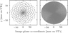Fig. 3. Examples of the scanning pattern applied in the Calibration Unit measurements. SC aberration maps were obtained with a slow modulation frequency (left). For the corresponding FT measurement, a faster scanning was used, and the right panel only shows a single iteration of in- and out-spiral.

In normal observation mode, GRAVITY controls the differential OPD between science channel and fringe tracker by its laser metrology and the common path to the telescopes by fringe tracking. During the phase map calibration measurement, however, fringe-tracking is not possible because the fringes are lost at the margins of the scanning region. Instead, the common path from the telescope to the instrument drifts in time. Thus the determination of the aberration pattern from the absolute FT and SC phase requires a drift correction. On the FT, the short detector integration time with maximum sampling frequency of 1 kHz allows us to resolve fast modulation of the source position, and the full FOV can be scanned within ∼15 s. Over this short time span, the drift is well described by a constant velocity, which we fitted and subtracted from the data. On the SC, in contrast, the minimum detector integration time is 0.13 s and a full scan of the FOV takes 2−3 min, which is too long to model the drift by a simple polynomial fit. Instead, we obtained the science channel aberrations via a detour and first analyzed the differential drift-free SC-FT phase. The pure science channel aberrations then follow from knowledge of the absolute fringe tracker phase.

The data were reduced by the standard GRAVITY pipeline, and we obtained the correlated flux in six FT spectral channels (ranging from 1.99−2.38 μm) and in medium resolution for the SC (233 wavelength bins in the range 1.97−2.48 μm). With the chosen setup, where the source position is varied on only one of the two beams forming a baseline, the measured correlated flux is given by

$$\begin{array}{c}\hfill {\langle {\eta }_i^{\mathit{ps}}\left({\mathit{\alpha }}_0\right){\left({\eta }_j^{\mathit{ps}}\left(\mathbf{0}\right)\right)}^{\ast }\rangle }_{\mathrm{obj}}=A_i\left({\mathit{\alpha }}_0\right)e^{i{\varphi }_i\left({\mathit{\alpha }}_0\right)}{A}_j\left(\mathbf{0}\right)e^{-i{\varphi }_j\left(\mathbf{0}\right)}.\end{array}$$(32)

Thus, the measurement directly scanned the phase- and amplitude-maps on the modulated channel. Potential offsets in the accompanying nonmodulated beam, ϕ_j(0) ≠ 0, can only cause a global phase shift, which we fitted and removed in the subsequent analysis. Finally, we considered the amplitude maps normalized to their maximum value, such that A_j(0) has no effect on our result.

In summary, we applied the following analysis steps to obtain the FT and the differential SC-FT phase- and amplitude-maps:

1. We fitted and subtracted a linear time drift from the phases measured in each spectral channel and on each baseline.

2. Phases and amplitudes were binned on a spatial grid with resolution 1 mas and averaged over all available periods of in- and out-spiral.

3. The image plane coordinates do not align perfectly with the amplitude maximum, that is, the source position for which the coupling to the fiber is most efficient. We corrected for this effect by fitting a Gaussian profile and shifting the coordinate origin to its maximum.

4. Interpolation over the gridded data provides the phase- and amplitude-map per spectral channel and baseline.

5. All spectral channels were combined into a single map at reference wavelength λ₀ = 2.2 μm by applying the approximate coordinate scaling from Eq. (14). We verified that the individual maps are consistent over the full spectral range. Cross-validation with simulated maps showed that the error introduced by the approximate scaling relation is small, except at the very margins of the map. It furthermore cancels out between channels above and below λ₀ to a very good degree.

6. From consideration of all baselines, three maps are available for each telescope. We again verified their consistency and averaged them into a single phase- and amplitude-map.

This method results in an FT and a differential SC-FT map for each telescope. Subtracting the former from the latter, we finally arrived at the desired SC phase map, which is shown in Fig. 4. The amplitude map on the SC, on the other hand, was measured directly.

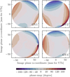Fig. 4. Science channel phase maps reconstructed by the procedure of Sect. 3.1 from the Calibration Unit measurement on 3 March 2020 for all four GRAVITY beams.

The Calibration Unit measurement was performed twice with a four-month break, in late 2019 and early 2020, and we use the data to construct two independent sets of maps. These agree very well in the qualitative features and structures they display. On the quantitative level, the maps display moderate differences of ∼10°, which are smaller at the center and increase toward the map margins.

3.2. Representation in the pupil plane

Analyzing the Calibration Unit measurement as described in the previous subsection, we obtain the phase- and amplitude-maps on a grid discretizing the image plane. We used this result to infer the underlying pupil-plane and fiber aberrations, d_pup(u) and d_foc(u), in their Zernike representation. To this end, we developed a simulation tool that creates complex maps of image-plane distortions from a set of Zernike coefficients according to Eqs. (5), (6), and (13).

For the fit we considered the two Calibration Unit measurements from 2019 and 2020 separately and combined the phase- and amplitude-maps for each telescope into a complex map. We then minimized the square absolute difference to the model prediction summed over all pixels with respect to the input coefficients. Because of the nature of the approximate coordinate scaling (step 5 of the analysis pipeline), at the edge of a map, only the smallest wavelengths contribute. We limited the radius to which the data are considered in the fit to α_max × λ_low/λ_high. Here, α_max is the size of the full map, and λ_low and λ_high are the wavelength of the lowest and highest channel, respectively. This choice ensures equal participation of all channels in the fit.

The optical layout of observations with the Calibration Unit has some important differences with the on-sky situation, for which the phase maps will be applied later: the lack of a central obscuration and an enlarged outer stop r_GCU = 9.6 m/2 alter the shape of the pupil defined in Eq. (4). As a consequence, the Calibration Unit pupil illuminates image-plane aberrations out to a slightly larger radius. We chose to normalize the Zernike polynomials by r_tel = 8.0/2 m, that is, the telescope area covered by the secondary mirror, to optimize our parameterization for the on-sky case. Image plane distortions, on the other hand, are normalized over the image-plane fiber width at λ₀, ${\stackrel{\sim }{\sigma }}_{\text{fib}}=ϵ{\lambda }_0/\left(4r_{\text{tel}}\sqrt{ln2}\right)$,

$$\begin{array}{c}\hfill d_{\mathrm{foc}}\left(\mathit{\alpha }\right)={\displaystyle \sum _{n=0}^{n_{\max }}\sum _{m=-n}^m{B}_n^m{Z}_n^m(\mathit{\alpha }/{\stackrel{\sim }{\sigma }}_{\mathrm{fib}}).}\end{array}$$(33)

Of the different types of maps we constructed, the fringe tracker provides the cleanest system and thus gives an important benchmark point for the agreement between model and data. We thus used the FT maps to determine the order n_max to which Zernike polynomials in the pupil- and focal-plane aberrations are considered. Successively increasing the fit order, we found that pupil-plane aberrations with n_max = 6 and focal-plane aberrations with n_max = 2 provide satisfactory model consistency while still allowing for manageable convergence times. Increasing the Zernike order in the pupil plane is especially important to reduce phase residuals at larger radii, while the central part of the maps can also be described by polynomials of lower order. Fits without focal-plane aberrations reproduce the phase structure to a satisfactory degree, but show poor consistency between the phase- and the amplitude-data. Finally, an additional parameter accounts for the overall amplitude scaling between measured and predicted maps, such that each fit constrains at least 34 degrees of freedom. The phase RMS achieved for the fringe tracker fits is ∼1° for all beams and data sets; extrapolation of the fit result to the full map radius yields an RMS of a few degrees.

In principle, it is possible to directly fit the SC maps by the same procedure employed for the FT. However, by further refining the analysis, we can remove additional systematic effects from the SC maps. When we created the maps, we corrected for misalignment of the image plane coordinates with the amplitude maximum (step 3 in the analysis pipeline). This shift, however, is not guaranteed to be identical on SC and FT, and as a result, there can be a small offset between the FT phase entering the differential SC-FT measurement. To describe this effect, we fitted a differential map, predicted from two sets of Zernike coefficients, to the SC-FT maps. The latter of these two sets of parameters was largely fixed to the previously obtained FT coefficients, and only the tip-tilt terms were allowed to vary. The SC parameters, on the other hand, were all left free, such that the fit eventually determined the desired SC maps and the offset between the two channels.

From the best-fit coefficients of the differential SC-FT fit, which we summarize in Appendix A, we constructed a complex SC map. Its phase is displayed in Fig. 5. As expected, the structure agrees very well with the maps obtained by direct evaluation of the Calibration Unit measurement in Fig. 4. Residuals between measured and fitted SC-FT map, shown in Fig. 6, are low over the full radius considered for the fit. We obtain a best-fit RMS of 1° −2° for most beams and data sets and two slightly worse results with RMS ∼3° and ∼5°. At larger radii, the disagreement between fit and data starts to increase. This can either be caused by wavelength-dependent errors or by higher order aberrations beyond those considered for the fit. When we optimized n_max, we noted indeed that every increase improved the extrapolation to large separations. However, at such large off-axis distances, fiber damping becomes very significant, resulting in a poor signal-to-noise ratio. We therefore consider the Zernike decomposition up to sixth order sufficient for our applications.

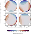Fig. 5. Science channel phase maps obtained from fits to the differential SC-FT maps, measured on 3 March 2020 for all four GRAVITY beams.

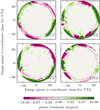Fig. 6. Phase residuals of the fit to the differential SC-FT map measured on 3 March 2020 for all four GRAVITY beams. Only the data within the dashed circle are considered in the fit; the cancellation of wavelength-dependent scaling errors is not guaranteed at larger radii.

4. Application to GRAVITY observations

Static field-dependent aberrations affect the visibility measurement whenever the size of an observed object is comparable to the fiber FOV. We applied the formalism developed in Sect. 2 alongside the characterization of aberrations from Sect. 3 to observations of two different binary systems. First we considered as a proof of concept a test-case binary observed with the Auxiliary Telescopes (ATs), where the system position in the FOV was systematically varied and thus screened over the phase- and amplitude-maps. Second we applied the aberration-correction to GC observations with the UTs from 2017 and 2018. During these epochs, which are around the pericenter passage of S2, S2 and Sgr A* where observed simultaneously in a single fiber pointing.

The data considered in either analysis consisted of visibility amplitudes, squared visibilities, and closure phases with a relative weighting of (1:1:2). To infer the source separations, we fit a binary model based on Eq. (25), which we extended to account for the effect of finite spectral resolution and for a homogeneous background with flux ratio f^bkg relative to the first binary component.

$$\begin{array}{cc}& V_{\mathrm{bin}}^{\mathrm{obs}}({\mathit{b}}_{i,j}/\lambda )\hfill \\ \hfill & =\frac{{\stackrel{\sim }{A}}_i\left({\mathit{\alpha }}_1\right){\stackrel{\sim }{A}}_j\left({\mathit{\alpha }}_1\right)V_{\lambda }[({\mathit{b}}_{i,j}·{\mathit{\alpha }}_1-{\mathit{d}}_{i,j}\left({\mathit{\alpha }}_1\right)),{\nu }_1]+{\stackrel{\sim }{A}}_i\left({\mathit{\alpha }}_2\right){\stackrel{\sim }{A}}_j\left({\mathit{\alpha }}_2\right)V_{\lambda }[({\mathit{b}}_{i,j}·{\mathit{\alpha }}_2-{\mathit{d}}_{i,j}\left({\mathit{\alpha }}_2\right)),{\nu }_2]}{\sqrt{\prod _{x=i,j}[{\stackrel{\sim }{L}}_x\left({\mathit{\alpha }}_1\right)V_{\lambda }(\mathbf{0},{\nu }_1)+f^{\mathrm{bin}}{\stackrel{\sim }{L}}_x\left({\mathit{\alpha }}_2\right)V_{\lambda }(\mathbf{0},{\nu }_2)+f^{\mathrm{bkg}}{V}_{\lambda }(\mathbf{0},{\nu }_{\mathrm{bkg}})]}}.\hfill \end{array}$$(34)

Phase distortions enter this expression via the OPD correction $d_{i,j}=({\stackrel{\sim }{\varphi }}_i-{\stackrel{\sim }{\varphi }}_j)\times \lambda /2\pi$. Furthermore, the point-source visibility averaged over a spectral channel is

$$\begin{array}{c}\hfill V_{\lambda }(\mathit{d},\nu )={\displaystyle \int }\mathrm{d}\lambda P\left(\lambda \right){\left(\frac{\lambda }{2.2\mu \mathrm{m}}\right)}^{-1-\nu }{e}^{-2\pi id/\lambda }.\end{array}$$(35)

The spectral bandpass P(λ) is given by a top hat function. The source positions α₁ and α₂, the flux ratios f^bin and f^bkg, and the spectral index of the central component (ν₁) and the background flux (ν_bkg) were free fit parameters, while the spectral slope of the companion was fixed to ν₂ = 3.

Finally, ${\stackrel{\sim }{A}}_{i/j}$, ${\stackrel{\sim }{\varphi }}_{i/j}$, and ${\stackrel{\sim }{L}}_{i/j}$ in Eq. (34) refer to the phase maps, amplitude maps, and the photometric lobes as they are encountered in on-sky observations. These have two important differences to the Calibration Unit measurement. First, while the pupil-plane representation of the aberrations is the same for both settings, the presence of a central obscuration and the smaller outer stop affects the realization of the maps in the image plane. This was conveniently captured by using the Zernike coefficients found in Sect. 3.2 to create a new set of maps with adjusted pupil configuration. Second, the maps are subject to turbulent smoothing according to Eqs. (30) and (31).

4.1. Verification for a binary test case

The test-case observations, carried out with the ATs in astrometric configuration, targeted HIP 41426, a binary with a K-band magnitude m_K ≃ 5.393 at RA = 8 : 26 : 57.75 h, Dec = −52 : 42 : 17.8 (Cutri et al. 2003). The system has an approximate separation of 200 mas. Its position relative to the GRAVITY fiber was kept fixed for three of the four telescopes and was varied in 24 steps between ±400 mas on AT2. At each offset, ten frames with a 6 s integration time were taken. The setup is illustrated in Fig. 7, which shows the two binary components relative to the fiber profile on all four telescopes. The shift was applied along the x-axis in the frame of the GRAVITY pupil, whose rotation with respect to the field results in a diagonal movement on the sky.

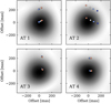Fig. 7. Illustration of the AT binary test observations, showing the position of the two binary components (circles and diamonds, respectively) relative to the fiber profile (gray shading). Color gradients are chosen in accordance with Fig. 8. For this test, the fiber position was only varied on AT2 and was kept fixed on the other three telescopes.

We used the Zernike coefficients obtained for the SC in Sect. 3.2 to produce phase- and amplitude-maps tailored to observations with the ATs. In this case, the pupil, cf. Eq. (4), is defined by r_tel = 1.82 m/2 and r_cent = 0.14 m/2. After beam collimation, ATs and UTs illuminate the same section on the GRAVITY mirrors, such that the pupil-plane phase screen can simply be scaled to the AT radius, that is, r_tel = 1.82 m/2 also applies in the Zernike decomposition of Eq. (5). To authenticate the effect of correct aberration modeling, we compared our results to a second no-map analysis. In this latter scenario, we set all phase maps to zero and all amplitude maps to one, ${\stackrel{\sim }{\varphi }}_{i/j}=0$, ${\stackrel{\sim }{A}}_{i/j}=1$.

For fiber offsets that are too large, the signal-to-noise ratio on AT2 is poor because of the high fiber damping, and we consequently discarded these data. The remaining pointings are shown in Fig. 7, and the corresponding separation, measured from a binary fit to the data according to Eq. (34), is given in Fig. 8.

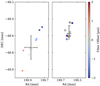Fig. 8. Binary separation inferred for a varying fiber offset on AT2 with (right panel) and without (left panel) application of the phase- and amplitude-maps. Each data point shows the average over two polarization states, and the range of offsets corresponds to ±200 mas, approximately.

The AT binary test case clearly validates our aberration corrections. Different configurations yield consistent results only if phase- and amplitude-maps are considered in the analysis. Including the correct aberration model in the analysis clearly shifts the result and reduces the scatter. Even more importantly, however, the separation found in the no-map analysis systematically depends on the fiber position; it is largest for positive fiber-offsets and smallest for offsets in the negative direction. When the aberration correction is applied, this systematic is largely removed.

We considered the binary test-case observations primarily as a proof of concept and therefore did not apply a full analysis of the systematic measurement error as carried out for the GC. These uncertainties arise from the accuracy to which the phase maps can be determined and from the uncertainty of the atmospheric smoothing kernel. Furthermore, there can be minor differences in the phase- and amplitude-maps between AT und UT observations, and our treatment is optimized for the UT scenario.

As the shift in its central value indicates, the binary separation is large enough that even at perfect fiber pointing, at least one source lies in a region of the FOV where aberration-induced phase errors are significant. Accurate astrometry is thus not a question of precise fiber alignment, but is only possible with a consistent treatment of the pupil-plane distortions in the analysis.

4.2. Separation between S2 and Sgr A*

After verifying our approach to correct for aberration-induced systematic errors, we also applied it to GC observations with GRAVITY. During 2017 and 2018, that is, close to pericenter passage, S2 and Sgr A* were observed simultaneously in a single fiber pointing. In particular during 2017, when the off-axis distance of S2 was larger, the aberration correction improves the inferred binary separation. In 2019, in contrast, the Sgr A*-S2 separation exceeded the single telescope beam size of about 60 mas, and GRAVITY observed both sources separately in so-called dual-beam mode. Their separation is then obtained by calibrating Sgr A* with S2 and fitting a point-source model to its visibilities (see Gravity Collaboration 2020 for details). In this configuration, each source can be well aligned with the fiber center, such that field-dependent aberrations do not affect the measurement.

To derive the aberration-induced shift of the S2 position, we examined a subset of the GRAVITY data used in Gravity Collaboration (2019). In particular, we applied stricter quality cuts and demanded a high signal-to-noise ratio. Phase- and amplitude-maps were generated from the coefficients obtained in Sect. 3.2 by accounting for the specific geometry of UT observations, that is, r_tel = 8.0 m/2 and r_cent = 0.96 m/2. The residual turbulent tip-tilt is between 10 mas and 15 mas per axis (Perrin & Woillez 2019). In total, we considered four different realizations of the aberration maps that are given by the independent analysis of the two calibration measurements in 2019 and 2020 each convolved with the minimum and maximum smoothing assumption. A representative example for the phase maps applied in the GC analysis is shown in Fig. 9 in relation to the orbit of S2.

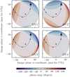Fig. 9. Orbit of S2 relative to the phase maps as applied for the GC analysis (measurement from 3 March 2020, σt = 10 mas). Dots indicate the position of S2 on 2017.2, 2017.6, 2018.2, and 2018.7, respectively, while the cross marks Sgr A*.

Our main result, the difference in the position of S2 with and without aberration corrections averaged per month, is shown in Fig. 10. As expected, the correction is largest early in 2017 and smallest around pericenter passage in May 2018. Furthermore, the mean corrections per epoch obtained with the four different realizations of the aberration maps are consistent over the full observational period.

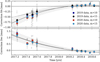Fig. 10. Difference in the position of S2 obtained from an analysis with and without the aberration corrections. Colored dots indicate the epoch-wise mean for different realizations of the phase- and amplitude-maps, and gray dots show the results for individual observations. From these, we determine a mean position correction as a function of time with a corresponding upper and lower limit as indicated by the solid black line and the gray band. The thin dashed line finally represents the correction applied in Gravity Collaboration (2019).

As the orbit of S2 smoothly scans over the phase- and amplitude-maps (see Fig. 9), we also expect a smooth variation in the position-correction. The time-dependence in Fig. 10 is indeed well described by a second-order polynomial fit,

$$\begin{array}{cc}\hfill \mathrm{\Delta }\mathrm{RA}& =(-0.44{\tau }^2+0.11\tau +0.04)\mathrm{mas},\hfill \end{array}$$(36)

$$\begin{array}{cc}\hfill \mathrm{\Delta }\mathrm{Dec}& =(0.41{\tau }^2-0.47\tau -0.06)\mathrm{mas},\hfill \end{array}$$(37)

where τ = t/years − 2018.4 refers to the shifted observation date in years.

In addition to the mean correction per epoch, Fig. 10 also shows the individual file-by-file results as gray dots. These give some insight into the uncertainty of the aberration correction. When we fit the orbit of S2, any such uncertainty must to be propagated as a source of systematic error. We constructed a upper and a lower estimate of the correction, containing 68% of the files per epoch. This is shown in Fig. 10 as a gray band.

In addition to the systematic error, we also need to account for the statistical uncertainty of the position of S2. That is, as the phase- and amplitude-error changes when the position of S2 is varied within its error bars, we need to propagate this effect to the final correction. To this end, we took the position error of the original uncorrected data point, from which we drew 100 realizations, and shifted the aberration maps by this. We then derived the correction from each realization independently and used their scatter to estimate the statistical error of the correction for the position of S2. The resulting mean statistical uncertainty per epoch is small, between 10 μas and 30 μas, but we nevertheless also accounted for it in the orbit fitting.

A further check was to determine which correction created a best match of the 2017 and 2018 GRAVITY positions to the remaining S2 data. To this end, we included a scaling factor f_corr in the correction we applied, such that f_corr = 1 was our best correction and f_corr = 0 was no correction. This parameter was then included in the orbit fit (see Sect. 5.1). The best fit yields f_corr = 0.99 ± 0.06, which is identical to the correction we derived purely from calibration data. This independently confirms our concept and the resulting aberration correction: Our correction yields the most consistent S2 orbit.

The aberration correction presented here constitutes a further refinement of the analysis in Gravity Collaboration (2020). There we directly applied the measured aberration maps as shown in Fig. (4) instead of the fitted decomposition in terms of pupil-plane Zernike polynomials. To account for the widening of the maps, which occurs when we project from the enlarged stop on the Calibration Unit to the telescope pupil, we applied a wider smoothing kernel of σ_t = (19±5) mas. The resulting best estimate for the correction is depicted in Fig. 10 as a dashed line. Both methods give consistent results, which confirms the robustness of the approach. The only sizable deviation is in 2017.2, when S2 was observed at a separation comparable to the maximum radius for which we obtained the calibration measurement (see Fig. 9). This case shows the strength of the Zernike decomposition, which allows a well-defined extrapolation.

5. Results

5.1. Determination of the S2 orbit

In the following we evaluate the effect of the aberration correction on the S2 orbit. The data used are similar to those of Gravity Collaboration (2020) and are described in detail in Appendix B. We employed the same fitting procedure as in Gravity Collaboration (2020), using a 13-parameter post-Newtonian orbit model. Six of these parameters describe the Kepler orbit (a, e, i, ω, Ω, and t_peri), and another six describe the reference frame relative to the AO spectroscopy and assumed correction for the local standard of rest (LSR) (x₀, y₀, R₀, ẋ₀, ẏ₀, ż₀). Here, R₀ is the distance to the GC, the prime focus of this work, and M_• is the central mass. The best-fit parameters are given in Table 2.

To determine the systematic uncertainty, we followed the approach in Gravity Collaboration (2019) of varying our assumptions and tracing the associated changes in R₀. Compared to our earlier work, we also included the uncertainty due to the aberration correction, as given by the gray band in Fig. 10. The individual contributions are given in Table 1. The aberration correction is the dominant contributor to the systematic error. The total systematic uncertainty is 33 pc when the contributions are added quadratically.

Our best estimate of the GC distance thus is

$$\begin{array}{c}\hfill R_0=8275\pm {9|}_{\mathrm{stat}.}\pm {33|}_{\mathrm{sys}.}\mathrm{pc}.\end{array}$$(38)

5.2. Comparison to previous results

Our previous determinations of the GC distance in Gravity Collaboration (2018, 2019), and Gravity Collaboration (2020) were biased by the field-dependent aberrations. Taking them into account brings all our measurements into agreement, as shown in Fig. 11 and Table 3. In contrast to Gravity Collaboration (2020), we here also applied a correction for the 2018 data, when S2 and Sgr A* were close to each other and close to the field center. We note that, the small aberration corrections lead to a small upward correction of R₀ of around 30 pc. However, this shift is comparable to the systematic error. Further, we find that the orbit is particularly sensitive to the pericenter data. This causes a strong decrease in the statistical uncertainty with time, while the systematic uncertainty even increases slightly because varying the assumptions then leads to stronger variations in the fit result.

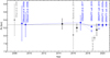Fig. 11. Measurements of the GC distance over time with a focus on studies of the S2 orbit. Blue points show results obtained with the SINFONI, NACO, and GRAVITY data with (dark blue) and without (light blue) application of the aberration corrections. Gray R0 determinations are based on data from the Keck observatory. For comparison, we show in black results that are based on the statistical parallax of the nuclear star cluster (Chatzopoulos et al. 2015) and from modeling the Milky Way dynamics based on observations of molecular masers (Reid et al. 2019). Bland-Hawthorn & Gerhard (2016) finally reported the GC distance based on a combination of various methods.

5.3. Comparison with further S2-based results

We estimate that the accuracy of our VLT-based result is at the 40 pc level. However, it deviates significantly from the Keck-based value reported in Do et al. (2019), with the difference being at the 300 pc level. Because both works use the orbit of S2 around Sgr A* to determine R₀, it is important to investigate the cause of the discrepancy, and we address this in Appendix C. Overall, we conclude that the combination of a difference in the radial velocity data and a modest offset of the Keck coordinate system in the declination direction might explain the discrepancy. Each effect contributes roughly 50%.

About 20% of the radial velocity difference can be attributed to the Doppler formula in StarKit that was implicitly used by Do et al. (2019). The remaining 80% are unexplained and might lie either in the Keck or the VLT data.

The origin of the coordinate system offset is unclear as well. Trying to explain the offset with a shift in the VLT coordinate systems is much harder than imposing a shift in the Keck system because the precision of the GRAVITY data is so high.

6. Conclusions

GRAVITY delivers high-resolution astrometry, which in combination with spectroscopic data, allows a very precise determination of the distance to the Galactic Center. The values inferred from different epochs (Gravity Collaboration 2018, 2019, 2020) show a small discrepancy at the 1% level, which nevertheless is significant because of the high precision of the measurement.

We were able to relate this shift to optical aberrations introduced in the instrument, which lead to a field-dependent distortion of the visibility phase. Their effect is stronger the farther off-axis an object lies within the FOV. In particular, GC observations close to the S2 pericenter passage are affected, when S2 and Sgr A* are detected simultaneously in a single fiber pointing but at a separation comparable to the FOV. In earlier and later epochs, in contrast, we employed the so-called dual-beam method and targeted each source individually. In this case, as for most other GRAVITY science observable, each source can be well centered and aberration corrections become irrelevant. The dual-beam observation mode was also assumed to derive the astrometric error budget in Lacour et al. (2014), who did not include the effect of phase maps for this precise reason.

The full analytical description we developed here allowed us to propagate the effect of optical aberrations at fiber injection to the measured visibilities. Fitting this model to dedicated calibration measurements confirmed its validity and enabled us to account for the effect in the data analysis. We further verified the approach with dedicated test-case observations.

The formalism we developed is applicable beyond GRAVITY to any optical/near-IR interferometer in which aberrations are introduced in the pupil or the focal plane. In several cases in the literature, more than one object lay in the interferometer FOV, for example, some Keck (Colavita et al. 2013), CHARA (Ten Brummelaar 2005), or NPOI (Armstrong et al. 1998) results on binary stars. How severely aberrations affect an observation depends not only on their strength for a particular instrument, however, but also on the off-axis distance considered and on the statistical noise in the measurement. In the example of GRAVITY on the UTs, the mean phase error introduced at 20 mas separation is 4−5 degrees per telescope and increases to 14−20 degrees at 50 mas. While a binary test case as presented in Sect. 4.1 can serve as a general strategy to diagnose whether aberration-induced systematics are a problem, dedicated calibration measurement are required for their correction in the analysis for each individual instrument.

With the results from the GRAVITY Calibration Unit measurements and our refined analysis scheme, we were able to further improve the separation between S2 and Sgr A* in 2017 and 2018, introducing shifts up to 0.5 mas caused by the phase aberrations. In Fig. 12 we show a detailed view of the S2 orbit in 2017, in which we also included two dual-beam measurements that do not suffer from phase aberrations. The improved data agrees very well with these positions.

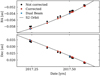Fig. 12. Detailed view of the S2 orbit in 2017. Dual-beam points do not suffer from aberration-related systematic errors and agree very well with our corrected data points.

Of all orbital parameters, the distance to the GC R₀ is most strongly affected by the change in the S2 position. This can be easily understood when R₀ is viewed as the scaling factor between angular and proper velocity. The field-dependent phase errors discussed in this work then fully explain the shift between earlier R₀ measurements with GRAVITY data. Applying the analysis scheme developed here lifts any such discrepancies (see Sect. 5.2). In particular, Fig. 11 demonstrates that later corrected data sets of earlier publications give fully consistent results whose accuracy increases with time.

References

Appendix A: List of Zernike coefficients

The Zernike coefficients obtained by fitting the Calibration Unit measurements from late 2019 and early 2020 are summarized in Tables A.1 and A.2, respectively. We provide the science channel results for all for GRAVITY beams (GV1 to GV4) in units of μm according to the definitions in Eqs. (5) and (33), where $A_n^m$ labels pupil-plane aberrations and $B_n^m$ those in the focal plane.

Appendix B: Data

We used the data set presented in Gravity Collaboration (2020) with the following changes. Each single-beam astrometric position was corrected according to Eq. (37), and we added the statistical error of this correction in quadrature, which increased the individual uncertainties by around 15 μas. Further, we corrected the radial velocity of the epoch 2018.1277, which was 13 km s⁻¹ too high in the previous data set. Finally, we were able to add one interferometric position measurement of S2 from early March 2020. Like in 2019, the separation between S2 and Sgr A* exceeds the fiber FOV, and hence a dual-beam measurement needed to be employed.

Because the observability of the GC is limited in early March and we expected observations in the following months, we did not attempt to observe Sgr A* in March 2020, but only pointed to S2 and to our usual calibrator star R2, with the aim of testing the stability of the GRAVITY astrometry. Pointings to Sgr A* were planned for later in the year. They had to be canceled due to the pandemic-related closure of the VLT(I) from mid-March on. To still determine the S2 – Sgr A* separation vector from this observation, we needed to proceed in two steps and first measured the S2 – R2 distance, then we referenced R2 to Sgr A*.

The distance between S2 and R2 was measured with the dual-beam method (Sect. 4.2), where we calibrated the S2 files with R2. In addition to the 2020 measurement, this separation is also available for 56 epochs in 2017, 2018, and 2019. It can be measured very precisely because the two stars are bright. Because the S2 – Sgr A* vectors were previously determined in Gravity Collaboration (2020), we can also refer R2 to Sgr A* in these earlier epochs. We then fit a simple quadratic function for the time evolution of the R2 coordinates relative to Sgr A* and extrapolated it to March 2020. Given the large number of data and the small time range to extrapolate for, the additional uncertainty that this introduces is well below the 100 μas level.

We derived the S2 position in 2020 from the four scientifically usable exposures as their mean. We assigned an error of 150 μas to each coordinate for this data point, which reflects both the smaller number of files compared to what we typically had available in 2019 and the additional uncertainty due to the additional step of referencing via R2. The new data point falls well onto the expected orbit, but its error bar is too large to have a significant effect on the fitted parameters.

Our data set consists of 128 AO-based astrometric points, 58 GRAVITY-based astrometric points, and 97 radial velocities, of which the first three before 2003 are from Do et al. (2019).

Appendix C: Analysis of the difference between R₀ determinations from Keck and VLT data sets

We expect that our determination of R₀ is accurate to the 40 pc level, but we note that the value published in Do et al. (2019) is discrepant at the 300 pc level. Both teams used the orbit of the star S2 around Sgr A* to determine R₀, and it is therefore natural to ask what caused the differences.

C.1. Data

In addition to our (VLT) data set (Appendix B), we used the Keck data set published in Do et al. (2019). We applied the NIRC2 radial velocity offset of +80 km s⁻¹ as determined in Do et al. (2019) to the NIRC2 data, that is, we added 80 km s⁻¹ to these radial velocities. Unlike Do et al. (2019), we then did not fit for this offset. Furthermore, we dropped the last astrometric data point (epoch 2018.67148268), as suggested by the authors in a private communication. The data set consisted of 45 astrometric points and 116 radial velocities, of which 41 are actually from the VLT data set between 2003 and 2016. The published table also includes one radial velocity from the epoch 2019.3567, which may not have been part of the data set used in Do et al. (2019).

C.2. Difference in R₀

We fit the orbit with a simple 13-parameter model: The six orbital elements of the star (corresponding to the initial conditions of the star in phase space), six parameters for the position and velocity of the MBH, and the mass of the MBH. The fits were made using the relativistic corrections as in Gravity Collaboration (2020), that is, we fixed f_RS = f_SP = 1. For this non-Keplerian motion, the meaning of the orbital elements is that they osculate at a reference epoch, for which we chose T = 2010.35, which is close to the apocenter passage time of S2.

To fit the VLT data set, we used the same approach as in Gravity Collaboration (2020): for the GRAVITY data, we assumed that the astrometry directly refers the S2 positions to the mass center and we directly measure the separation vector between the two objects interferometrically. For the NACO (AO-imaging based) data, we allowed a coordinate system offset, on which we set priors following Plewa et al. (2015), and we included the NACO flare positions as an additional constraint to locate the mass. This fit yields

$$\begin{array}{cc}& R_0=8274.9\pm 9.3\mathrm{pc}\hfill \\ \hfill & a=124.982\pm 0.034\mathrm{mas}\hfill \\ \hfill & i=134.685\pm 0.{029}^{°}\hfill \\ \hfill & \mathrm{\Omega }=227.175\pm 0.{029}^{°},\hfill \end{array}$$(C.1)

where a is the semimajor axis, i is the inclination, and Ω is the position angle of the ascending node of the S2 orbit, and the errors are the statistical fit uncertainties. The VLT astrometry is dominated by the GRAVITY points, as illustrated by dropping all AO data points, which results in R₀ = 8276 ± 10 pc.

Fitting the Keck data set with the same 13-parameter model as used for Eq. (C.1) yields

$$\begin{array}{cc}& R_0=7935\pm 44\mathrm{pc}\hfill \\ \hfill & a=126.64\pm 0.27\mathrm{mas}\hfill \\ \hfill & i=133.78\pm 0.{15}^{°}\hfill \\ \hfill & \mathrm{\Omega }=227.66\pm 0.{13}^{°}.\hfill \end{array}$$(C.2)

This is not the same number as in Do et al. (2019), who reported R₀ = 7959 ± 59 pc. The small (and statistically insignificant) difference is most likely due to the noise model that Do et al. (2019) included in their analysis, which we do not have readily available. Applying the noise model at hand (Plewa & Sari 2018; Gravity Collaboration 2019) yields R₀ = 7965 ± 56 pc. This shows that the value reported by Do et al. (2019) lies between the two numbers we obtain by refitting their data. In the following, we use for simplicity and for equal treatment of the data the value and approach as in Eq. (C.2). We therefore have a difference of ΔR₀ = 340 ± 45 pc.

C.3. Comparing, combining, and adjusting the astrometry

Gillessen et al. (2009a) have noted that a simple attempt of comparing the astrometric data sets by plotting them on top of each other fails. We need to allow for an offset and a drift between the two coordinate systems (i.e., four parameters Δx,  Δy,  Δv_x, and  Δv_y). This yields a 17-parameter fit. Comparing the best-fitting parameters in Eqs. (C.1) and (C.2) shows that they differ significantly in Ω. This parameter is fully degenerate with the angular orientation (called β here) of the coordinate system. The difference in Ω thus suggests that the two astrometric data sets are rotated with respect to each other.

Therefore we extend the combination scheme by an additional fifth parameter, Δβ, resulting in an 18-parameter fit. With this, we fit the two data sets simultaneously, omitting the 41 VLT radial velocities from the Keck data set while also dropping the three Keck velocities in the VLT data set. This fit matches the two coordinate systems ideally onto each other and results in

$$\begin{array}{cc}& R_0=8260\pm 9\mathrm{pc}\hfill \\ \hfill & a=125.00\pm 0.03\mathrm{mas}\hfill \\ \hfill & i=134.66\pm 0.{03}^{°}\hfill \\ \hfill & \mathrm{\Omega }=228.16\pm 0.{03}^{°}\hfill \\ \hfill & \mathrm{\Delta }\beta =0.32\pm 0.{05}^{°}.\hfill \end{array}$$(C.3)

The value of Δβ matches the difference ΔΩ. We conclude that the Keck and VLT data are indeed rotated with respect to each other. The other parameters are very similar to Eq. (C.1), which is due to the considerably smaller astrometric uncertainties of the GRAVITY data compared to the adaptive optics data.

With the best-fit coordinate system difference in hand, we can transform the Keck astrometric data into the VLT coordinate system and vice versa. We chose to do the former because the VLT data set is more directly calibrated by the interferometric data. After applying the coordinate system difference to the Keck data, we fit them again with a 13-parameter model. This yielded the same best-fit parameters as in Eq. (C.2) (with the exception of Ω). This shows that transforming the astrometry does not change the more fundamental differences between the two orbits, while a direct comparison is now feasible. The value of Ω can be omitted in the following.

C.4. Discrepancy in the radial velocity data

Chu et al. (2018) have investigated the consistency of the radial velocity data between the Keck and VLT data sets for 2000 to 2016 and concluded that the data agree with each other. We repeated the exercise, now also extending into the time of the pericenter passage in 2018 (Fig. C.1). To our surprise, the radial velocities differ systematically from ∼2011 on, and the difference increases as the radial velocity continues to increase. The difference reaches ∼50 km s⁻¹ in 2018, just before the star passed pericenter. Moreover, there is one obvious outlier in the Keck data, the earliest 2018 point. We verified that dropping this measurement does not change the Keck fit result in any significant way.

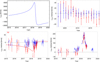Fig. C.1. Comparison of the radial velocity data sets. Blue points are data from the VLT data set, and red points are data from the Keck data set. Top left: radial velocity as a function of time for the VLT fit (Eq. (C.1)). Top right: yearly averages of the residua of the two data sets to the fit from Eq. (C.1). By construction, the VLT data thus scatter around 0. The Keck data deviate systematically from 2011 on, and the discrepancy increases in later years. Bottom left: same as the left panel, but zooming in to the period 2015–2020, and showing all individual data points. The best-fit Keck orbit corresponding to Eq. (C.2) is the red line. The difference is apparently largest when the radial velocity is highest (in 2018 at pericenter passage). Bottom right: both data sets show a clear peak in radial velocity in 2018 compared with the Keplerian part of the VLT fit (Eq. (C.1)), i.e., both data sets clearly detect the redshift term.

The obvious question is what the radial velocity effect is on R₀. To answer this, we swapped the radial velocities between the two data sets. The VLT set together with the Keck astrometry yields

$$\begin{array}{cc}& R_0=8094\pm 32\mathrm{pc}\hfill \\ \hfill & a=126.08\pm 0.21\mathrm{mas}\hfill \\ \hfill & i=134.0\pm 0.{13}^{°}.\hfill \end{array}$$(C.4)

Conversely, the Keck radial velocities together with the VLT astrometry yield R₀ = 8214 ± 14 pc. Because the Keck radial velocity set contains 35% of the VLT radial velocities, the fit in Eq. (C.4) is the cleaner test. We thus explain roughly half of the difference in R₀ with the radial velocity data, that is, 159 pc.

So far, we could only find an explanation for ∼20% of the radial velocity difference: We applied the fitting based on the stellar atmosphere model with the StarKit package used in Do et al. (2019) also to the VLT spectroscopy. We found a significant difference for high radial velocities, which we were able to trace back to the Doppler formula used by the StarKit package. While both Do et al. (2019) and Gravity Collaboration (2020) stated that the spectroscopic observable is v_r = z c, that is, the redshift of a given spectrum, the StarKit package applies a Doppler formula that includes the longitudinal relativistic correction: $\lambda \prime ={\lambda }_0\sqrt{\frac{1+{\mathit{v}}_{\mathrm{r}}/c}{1-{\mathit{v}}_{\mathrm{r}}/c}}$. In this form, the Doppler formula ignores the (significant) tangential motion v_t of S2. In order to apply a relativistic correction, the full Doppler formula $1+z=\frac{1+{\mathit{v}}_{\mathrm{r}}/c}{\sqrt{1-({\mathit{v}}_{\mathrm{r}}^2+{\mathit{v}}_{\mathrm{t}}^2)/c^2}}$ (Lindegren & Dravins 2003) is required. For this correction, however, the spectroscopic information is not sufficient. In general, a spectrum cannot be Doppler-corrected in a relativistic way without knowledge of the other motion component. Furthermore, even if the full correction were applied, it would be impossible to fit for the relativistic redshift later.

The difference between the two formulae is small at velocities far lower than the speed of light, but it becomes large close to pericenter, when S2 reaches a velocity of nearly 8000 km s⁻¹. It amounts to ∼25 km s⁻¹ at most, however, and thus is smaller than the observed difference in Fig. C.1. This difference is also visible in Fig. 1 of Do et al. (2019): The plotted model spectra are slightly more redshifted than the underlying data suggest. Changing the Keck radial velocities accordingly yields a fit with R₀ = 7972 ± 44 pc, which accounts for 37 pc of the 159 pc.

Further checks did not yield any clues for the remaining significant difference in the radial velocities. In this context, we verified whether the time stamps were assigned consistently between the two data sets, and did not find a difference. We also note that in the bottom right panel in Fig. C.1 the redshift peak around pericenter is clearly visible for both data sets.

C.5. Discrepancy in the astrometry

Comparison of the fits in Eqs. (C.1) and (C.2) shows that they differ not only in R₀, but also in the size of the semimajor axis a. We find Δa/a = 1.28 ± 0.22%. This does not hold for the semiminor axis, however, Δb/b is consistent with 0. Interestingly, the projected ellipses as given by the astrometric data in the plane of sky agree in both semimajor and semiminor axes to within 0.17%. Hence, the inclinations i need to differ, which Eqs. (C.1) and (C.2) confirm. We find in accordance with the above 1  −  sin(i_VLT)/sin(i_Keck) ∼ 1.3%.

The inclination of the ellipse determines where the projected center of mass is located. The orientation of the S2 orbit and the disagreement in a but not in b indicate an offset of the center of mass in the declination direction. We show that introducing an offset to either y or v_y (the mass position and velocity in declination) can indeed explain the remaining discrepancy. Starting from the fit of the transformed Keck data set, we fixed v_y to its best-fit value of −0.15 mas yr⁻¹. All other parameters were again left free for a subsequent fit. Additionally using the VLTI velocities in this fit instead of the Keck velocities yields

$$\begin{array}{cc}& R_0=8277\pm 28\mathrm{pc}\hfill \\ \hfill & a=124.76\pm 0.16\mathrm{mas}\hfill \\ \hfill & i=134.63\pm 0.{11}^{°}.\hfill \end{array}$$(C.5)

This fit therefore yields the same value for R₀ from the Keck astrometry as the VLT fit. Moreover, the semimajor axis a and inclination i have moved to the VLT values when v_y is forced to have an offset. Because the mass position is parameterized with a time origin at T = 2000.0, the best-fit y also changes, from −0.972 mas to 1.234 mas. The systematic uncertainty on y and v_y estimated by Do et al. (2019) is 1.16 mas and 0.066 mas yr⁻¹, respectively. This means that the difference that needs to be enforced is within ∼2σ of the systematic uncertainty, and the residuals in Fig. C.2 (left) appear to be acceptable. Essentially the same can be achieved by forcing an offset to y and leaving v_y free instead.

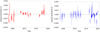Fig. C.2. Comparison of the astrometric residual after forcing an offset in declination such that the fit to the Keck data set matches that to the VLT (left) and such that the fit to VLT data set matches that to the Keck data (right). Lighter blue corresponds to AO data from the VLT data set, and darker blue to the GRAVITY data.

This argument might be reversed and a similar offset be applied to the VLT data in order to lower the VLT-based value of R₀. In a first attempt, we applied the same offset to the VLT AO data. However, even an offset 10 x larger (i.e., 1.2 mas yr⁻¹) changed R₀ by only ∼30 pc. This is expected because the VLT astrometry is completely dominated by the GRAVITY data. We therefore instead tried to vary v_y and y for the GRAVITY data, giving up the assumption that the GRAVITY source itself is the mass center. We also exchanged the VLT radial velocities for the Keck velocities. We find that we need to change v_y by −1.4 mas yr⁻¹ in order to obtain a similar distance to the Keck value:

$$\begin{array}{cc}& R_0=7928\pm 16\mathrm{pc}\hfill \\ \hfill & a=126.89\pm 0.05\mathrm{mas}\hfill \\ \hfill & i=133.51\pm 0.{03}^{°}.\hfill \end{array}$$(C.6)

The fit achieves the lower R₀ by tilting the orbit similar to the fit from Eq. (C.2). The enforced change of v_y is unrealistically large (12× larger than what was needed for the Keck data). The GRAVITY data also show very strong and systematic residuals of up to 0.5 mas (right panel in Fig. C.2), and the reduced χ² of the fit increased from 1.50 to 2.63.

All Tables

All Figures

Fig. 1. Schematic depiction of the pupil and focal plane aberrations that enter the overlap integral. Both effects in combination are required to describe the aberration patterns observed in calibration measurements. The lowest order aberrations in the pupil function are shown explicitly, which are (A) lateral fiber misplacement, (B) fiber tilt, and (C) defocus. Their effect is further explained in the text.

In the text

Fig. 2. Example phase screens (top) and amplitude maps (bottom) in the image plane induced by low-order Zernike aberrations in the pupil plane at a wavelength of λ0 = 2.2 μm. From left to right: the considered aberrations are a perfect Airy pattern, a vertical tilt of 0.4 μm RMS, a vertical astigmatism of 0.2 μm RMS, a vertical coma of 0.2 μm RMS, and a combination of astigmatism, coma, and trefoil (with RMS 0.2 μm, 0.2 μm, and 0.1 μm, respectively). The rightmost panel also considers an additional fiber tilt with 0.2 μm RMS.

In the text

	Fig. 3. Examples of the scanning pattern applied in the Calibration Unit measurements. SC aberration maps were obtained with a slow modulation frequency (left). For the corresponding FT measurement, a faster scanning was used, and the right panel only shows a single iteration of in- and out-spiral.
In the text

	Fig. 4. Science channel phase maps reconstructed by the procedure of Sect. 3.1 from the Calibration Unit measurement on 3 March 2020 for all four GRAVITY beams.
In the text

	Fig. 5. Science channel phase maps obtained from fits to the differential SC-FT maps, measured on 3 March 2020 for all four GRAVITY beams.
In the text

	Fig. 6. Phase residuals of the fit to the differential SC-FT map measured on 3 March 2020 for all four GRAVITY beams. Only the data within the dashed circle are considered in the fit; the cancellation of wavelength-dependent scaling errors is not guaranteed at larger radii.
In the text

	Fig. 7. Illustration of the AT binary test observations, showing the position of the two binary components (circles and diamonds, respectively) relative to the fiber profile (gray shading). Color gradients are chosen in accordance with Fig. 8. For this test, the fiber position was only varied on AT2 and was kept fixed on the other three telescopes.
In the text

	Fig. 8. Binary separation inferred for a varying fiber offset on AT2 with (right panel) and without (left panel) application of the phase- and amplitude-maps. Each data point shows the average over two polarization states, and the range of offsets corresponds to ±200 mas, approximately.
In the text

	Fig. 9. Orbit of S2 relative to the phase maps as applied for the GC analysis (measurement from 3 March 2020, σt = 10 mas). Dots indicate the position of S2 on 2017.2, 2017.6, 2018.2, and 2018.7, respectively, while the cross marks Sgr A*.
In the text

Fig. 10. Difference in the position of S2 obtained from an analysis with and without the aberration corrections. Colored dots indicate the epoch-wise mean for different realizations of the phase- and amplitude-maps, and gray dots show the results for individual observations. From these, we determine a mean position correction as a function of time with a corresponding upper and lower limit as indicated by the solid black line and the gray band. The thin dashed line finally represents the correction applied in Gravity Collaboration (2019).

In the text

Fig. 11. Measurements of the GC distance over time with a focus on studies of the S2 orbit. Blue points show results obtained with the SINFONI, NACO, and GRAVITY data with (dark blue) and without (light blue) application of the aberration corrections. Gray R0 determinations are based on data from the Keck observatory. For comparison, we show in black results that are based on the statistical parallax of the nuclear star cluster (Chatzopoulos et al. 2015) and from modeling the Milky Way dynamics based on observations of molecular masers (Reid et al. 2019). Bland-Hawthorn & Gerhard (2016) finally reported the GC distance based on a combination of various methods.

In the text

	Fig. 12. Detailed view of the S2 orbit in 2017. Dual-beam points do not suffer from aberration-related systematic errors and agree very well with our corrected data points.
In the text

Fig. C.1. Comparison of the radial velocity data sets. Blue points are data from the VLT data set, and red points are data from the Keck data set. Top left: radial velocity as a function of time for the VLT fit (Eq. (C.1)). Top right: yearly averages of the residua of the two data sets to the fit from Eq. (C.1). By construction, the VLT data thus scatter around 0. The Keck data deviate systematically from 2011 on, and the discrepancy increases in later years. Bottom left: same as the left panel, but zooming in to the period 2015–2020, and showing all individual data points. The best-fit Keck orbit corresponding to Eq. (C.2) is the red line. The difference is apparently largest when the radial velocity is highest (in 2018 at pericenter passage). Bottom right: both data sets show a clear peak in radial velocity in 2018 compared with the Keplerian part of the VLT fit (Eq. (C.1)), i.e., both data sets clearly detect the redshift term.

In the text

	Fig. C.2. Comparison of the astrometric residual after forcing an offset in declination such that the fit to the Keck data set matches that to the VLT (left) and such that the fit to VLT data set matches that to the Keck data (right). Lighter blue corresponds to AO data from the VLT data set, and darker blue to the GRAVITY data.
In the text

References

- Armstrong, J. T., Mozurkewich, D., Rickard, L. J., et al. 1998, ApJ, 496, 550 [Google Scholar]
- Bhatnagar, S., Cornwell, T. J., Golap, K., & Uson, J. M. 2008, A&A, 487, 419 [NASA ADS] [CrossRef] [EDP Sciences] [Google Scholar]
- Bland-Hawthorn, J., & Gerhard, O. 2016, ARA&A, 54, 529 [NASA ADS] [CrossRef] [EDP Sciences] [Google Scholar]
- Blind, N., Eisenhauer, F., Haug, M., et al. 2014, Proc. SPIE, 9146, 91461U [Google Scholar]
- Boehle, A., Ghez, A. M., Schödel, R., et al. 2016, ApJ, 830, 17 [Google Scholar]
- Chatzopoulos, S., Fritz, T. K., Gerhard, O., et al. 2015, MNRAS, 447, 948 [Google Scholar]
- Chu, D. S., Do, T., Hees, A., et al. 2018, ApJ, 854, 12 [Google Scholar]
- Colavita, M. M., Wizinowich, P. L., Akeson, R. L., et al. 2013, PASP, 125, 1226 [Google Scholar]
- Cutri, R. M., Skrutskie, M. F., van Dyk, S., et al. 2003, VizieR Online Data Catalog: II/246 [Google Scholar]
- Do, T., Hees, A., Ghez, A., et al. 2019, Science, 365, 664 [NASA ADS] [CrossRef] [Google Scholar]
- Eisenhauer, F., Genzel, R., Alexander, T., et al. 2005, ApJ, 628, 246 [Google Scholar]
- Genzel, R., Eisenhauer, F., & Gillessen, S. 2010, Rev. Mod. Phys., 82, 3121 [Google Scholar]
- Ghez, A. M., Duchêne, G., Matthews, K., et al. 2003, ApJ, 586, L127 [Google Scholar]
- Ghez, A., Salim, S., Weinberg, N. N., et al. 2008, ApJ, 689, 1044 [Google Scholar]
- Gillessen, S., Eisenhauer, F., Fritz, T. K., et al. 2009a, ApJ, 707, L114 [Google Scholar]
- Gillessen, S., Eisenhauer, F., Trippe, S., et al. 2009b, ApJ, 692, 1075 [NASA ADS] [CrossRef] [Google Scholar]
- Gillessen, S., Plewa, P. M., Eisenhauer, F., et al. 2017, ApJ, 837, 30 [Google Scholar]
- Gravity Collaboration (Abuter, R., et al.) 2017, A&A, 602, A94 [NASA ADS] [CrossRef] [EDP Sciences] [Google Scholar]
- Gravity Collaboration (Abuter, R., et al.) 2018, A&A, 615, L15 [NASA ADS] [CrossRef] [EDP Sciences] [Google Scholar]
- Gravity Collaboration (Abuter, R., et al.) 2019, A&A, 625, L10 [NASA ADS] [CrossRef] [EDP Sciences] [Google Scholar]
- Gravity Collaboration (Abuter, R., et al.) 2020, A&A, 636, L5 [CrossRef] [EDP Sciences] [Google Scholar]
- Habibi, M., Gillessen, S., Martins, F., et al. 2017, ApJ, 847, 120 [Google Scholar]
- Lacour, S., Eisenhauer, F., Gillessen, S., et al. 2014, A&A, 567, A75 [NASA ADS] [CrossRef] [EDP Sciences] [Google Scholar]
- Lindegren, L., & Dravins, D. 2003, A&A, 401, 1185 [NASA ADS] [CrossRef] [EDP Sciences] [Google Scholar]
- Martins, F., Gillessen, S., Eisenhauer, F., et al. 2008, ApJ, 672, L119 [NASA ADS] [CrossRef] [Google Scholar]
- Neumann, E. G. 1988, Single-mode Fibers [Google Scholar]
- Perrin, G., & Woillez, J. 2019, A&A, 625, A48 [NASA ADS] [CrossRef] [EDP Sciences] [Google Scholar]
- Pfuhl, O., Haug, M., Eisenhauer, F., et al. 2014, Proc. SPIE, 9146, 914623 [Google Scholar]
- Plewa, P. M., & Sari, R. 2018, MNRAS, 476, 4372 [Google Scholar]
- Plewa, P. M., Gillessen, S., Eisenhauer, F., et al. 2015, MNRAS, 453, 3234 [Google Scholar]
- Reid, M. J., Menten, K. M., Brunthaler, A., et al. 2019, ApJ, 885, 131 [Google Scholar]
- Roddier, F. 1981, Prog. Opt., 19, 281 [Google Scholar]
- Smirnov, O. M. 2011, A&A, 527, A107 [NASA ADS] [CrossRef] [EDP Sciences] [Google Scholar]
- Smirnov, O. M., & Tasse, C. 2015, MNRAS, 449, 2668 [NASA ADS] [CrossRef] [Google Scholar]
- Tasse, C., Hugo, B., Mirmont, M., et al. 2018, A&A, 611, A87 [NASA ADS] [CrossRef] [EDP Sciences] [Google Scholar]
- Ten Brummelaar, T. A., et al. 2005, ApJ, 628, 453 [Google Scholar]
- Wallner, O., Leeb, W. R., & Winzer, P. J. 2002, J. Opt. Soc. Am. A, 19, 2445 [Google Scholar]