| Issue |
A&A
Volume 647, March 2021
|
|
|---|---|---|
| Article Number | A46 | |
| Number of page(s) | 18 | |
| Section | The Sun and the Heliosphere | |
| DOI | https://doi.org/10.1051/0004-6361/202039107 | |
| Published online | 05 March 2021 | |
The influence of NLTE effects in Fe I lines on an inverted atmosphere
II. 6301 Å and 6302 Å lines formed in 3D NLTE
1
Max-Planck-Institut für Sonnensystemforschung, Justus-von-Liebig-Weg 3, 37077 Göttingen, Germany
e-mail: This email address is being protected from spambots. You need JavaScript enabled to view it.
2
Institute of Particle Physics and Astrophysics, ETH Hönggerberg, 8093 Zürich, Switzerland
3
School of Space Research, Kyung Hee University, Yongin, Gyeonggi 446-701, Republic of Korea
Received:
5
August
2020
Accepted:
29
December
2020
Abstract
Context. This paper forms the second part of our study of how neglecting non-local thermodynamic equilibrium (NLTE) conditions in the formation of Fe I 6301.5 Å and the 6302.5 Å lines affects the atmosphere that is obtained by inverting the Stokes profiles of these lines in LTE. The main cause of NLTE effects in these lines is the line opacity deficit that is due to the excess ionisation of Fe I atoms by ultraviolet (UV) photons in the Sun.
Aims. In the first paper, these photospheric lines were assumed to have formed in 1D NLTE and the effects of horizontal radiation transfer (RT) were neglected. In the present paper, the iron lines are computed by solving the RT in 3D. We investigate the effect of horizontal RT on the inverted atmosphere and how it can enhance or reduce the errors that are due to neglecting 1D NLTE effects.
Methods. The Stokes profiles of the iron lines were computed in LTE, 1D NLTE, and 3D NLTE. They were all inverted using an LTE inversion code. The atmosphere from the inversion of LTE profiles was taken as the reference model. The atmospheres from the inversion of 1D NLTE profiles (testmodel-1D) and 3D NLTE profiles (testmodel-3D) were compared with it. Differences between reference and testmodels were analysed and correspondingly attributed to NLTE and 3D effects.
Results. The effects of horizontal RT are evident in regions surrounded by strong horizontal temperature gradients. That is, along the granule boundaries, regions surrounding magnetic elements, and its boundaries with intergranular lanes. In some regions, the 3D effects enhance the 1D NLTE effects, and in some, they weaken these effects. In the small region analysed in this paper, the errors due to neglecting the 3D effects are lower than 5% in temperature. In most of the pixels, the errors are lower than 20% in both velocity and magnetic field strength. These errors also persist when the Stokes profiles are spatially and spectrally degraded to the resolution of the Swedish Solar Telescope (SST) or Daniel K. Inouye Solar Telescope (DKIST).
Conclusions. Neglecting horizontal RT introduces errors not only in the derived temperature, but also in other atmospheric parameters. The error sizes depend on the strength of the local horizontal temperature gradients. Compared to the 1D NLTE effect, the 3D effects are more localised in specific regions in the atmosphere and are weaker overall.
Key words: radiative transfer / line: formation / line: profiles / Sun: magnetic fields / Sun: photosphere / Sun: atmosphere
© H. N. Smitha et al. 2021
 Open Access article, published by EDP Sciences, under the terms of the Creative Commons Attribution License (https://creativecommons.org/licenses/by/4.0), which permits unrestricted use, distribution, and reproduction in any medium, provided the original work is properly cited.
Open Access funding provided by Max Planck Society.
1. Introduction
The nature of the radiative transfer (RT) problem for any stellar atmosphere diagnostic is inherently multi-dimensional and coupled with the effects of non-local thermodynamic equilibrium (non-LTE). For the solar atmosphere, one of the early studies in which the two-dimensional (2D) RT problem was solved was in the construction of a spicule model by Avery & House (1969) based on the Ca II K line. This was followed by Cannon (1970), Cannon & Rees (1971), Avrett & Loeser (1971), and Cannon (1971) among others, who solved the 2D transfer equation to study the solar chromosphere, derive solar atmospheric models, and so on. Stenholm (1977), Stenholm & Stenflo (1977, 1978) studied the effects of horizontal irradiation on Stokes profiles in magnetic flux tubes by solving the 2D transfer equation in cylindrical geometry. For a detailed review, see Carlsson (2008).
A few years later, Nordlund (1985) for the first time studied the spectral line formation in 3D with NLTE effects in a realistic 3D model atmosphere. Since then, 3D NLTE computations on 3D model atmospheres have been used to compute spectral lines of, for example, lithium (Asplund et al. 2003), oxygen (Kiselman & Nordlund 1995; Asplund et al. 2004, 2005; Pereira et al. 2009; Prakapavičius et al. 2013; Steffen et al. 2015), iron (Lind et al. 2017), manganese (Bergemann et al. 2019), and barium (Gallagher et al. 2020) to determine their abundances in solar and other stellar atmospheres. Recently, forward-modeling of chromospheric lines such as the Ca II 8542 Å line (Leenaarts et al. 2009), the Na I D1 line (Leenaarts et al. 2010), the Hα line (Leenaarts et al. 2012, 2015), the Mg II h and k lines (Leenaarts et al. 2013), and the Ca II H and K lines (Anusha & Nagendra 2013; Bjørgen et al. 2018) were carried out in 3D NLTE to understand the line formation and to study different chromospheric features that are observed with these lines. Sukhorukov & Leenaarts (2017) synthesized the Mg II h and k, Lyα, and Lyβ lines taking the complexities of partial frequency redistribution in 3D NLTE into account. Bergemann et al. (2019) modelled different chromospheric lines observed in active regions using 3D NLTE computations.
We focus on the 3D NLTE effects in the Fe I 6301.5 Å and 6302.5 Å lines that are formed in a network region. Although their line core formation height is in the upper photosphere, they are affected by the NLTE conditions in the atmosphere. This is because of the over-ionisation of the Fe I atoms by the ultraviolet (UV) photons. This underpopulation of Fe I atoms results in a line opacity deficit and decreases the departure coefficient to a value below unity. Because of their formation height, the lines are also affected by the source function deficit. Depending on which of the two effects dominates, the NLTE lines are either weaker or stronger than the LTE lines. These effects have now been known for more than four decades and are discussed by Athay & Lites (1972), Rutten & Kostik (1982), Rutten et al. (1988), Solanki & Steenbock (1988), and Shchukina & Trujillo Bueno (2001), to name a few. In all these papers, the RT equation was solved in 1D and the effects of multi-dimensions were neglected. In a series of papers, Holzreuter & Solanki (2012), Holzreuter & Solanki (2013), and Holzreuter & Solanki (2015) for the first time computed the photospheric iron lines at 5247 Å, 5250 Å, 6301.5 Å, and 6302.5 Å in 3D NLTE using different model atmospheres: a simple flux tube model, a 3D hydrodynamic (HD) simulation, and a 3D magnetohydrodynamic (MHD) simulation. They presented a detailed comparison of the Stokes profiles computed in LTE, 1D NLTE, and 3D NLTE and highlighted the importance of accounting for the 3D NLTE effects in these lines. However, no comparison with observations was made. Lind et al. (2017) modelled the observed centre-to-limb variation in intensity for many iron lines, different from the above four, by solving the RT in 3D NLTE and measured the solar iron abundance.
Because the Fe I 6301.5 Å and 6302.5 Å lines are extensively used for solar photospheric diagnostics, it is important to account for the multi-dimensional NLTE effects in their analysis. The routinely employed Stokes profiles inversions assume that the lines are formed in LTE, which is always 1D in diagnostic RT. Neglecting the 3D NLTE effects introduces errors in the derived atmospheric model. Understanding by how much the 3D NLTE effects affect the inverted atmosphere is the main aim of the present study. In the first paper of this series, we assumed the iron lines to be formed in 1D NLTE conditions and estimated the errors in the atmosphere derived by inverting their Stokes profiles using an LTE inversion code (Smitha et al. 2020, hereafter paper I). We found that neglecting the 1D NLTE effects introduces errors in the measurement of all atmospheric parameters. In the temperature, the errors can be as large as 13%, and in the line-of-sight (LOS) velocity and magnetic field strength, the errors can reach 50% or more. Even the measurement of the magnetic field inclination is prone to errors when 1D NLTE effects are neglected. These effects were evident in Stokes profiles in granules, intergranular lanes, magnetic elements, their boundaries, basically in every region with strong vertical gradients in temperature, in the LOS velocity, or in the magnetic field.
In this second paper of this series, we account for the horizontal RT effects in the iron lines and investigate how they affect the inverted atmosphere. Similar to Paper I, we compute the Stokes profiles in LTE and 3D NLTE conditions, and invert them using an LTE inversion code. The LTE inversion of LTE profiles is self-consistent, and we treat the derived atmospheric model as a reference. The inverted atmosphere from the LTE inversion of 3D NLTE profiles is not self-consistent, so that any departures with respect to the reference model can be attributed to the 3D NLTE effects. More details of this approach are discussed in the sections below. As discussed in Holzreuter & Solanki (2012, 2013, 2015), the horizontal RT effects can either weaken or strengthen the 1D NLTE effects. We investigate by how much the 3D effects strengthen or weaken the 1D NLTE effects and thus increase or decrease the errors in the inverted atmosphere.
2. Radiative transfer computations
2.1. Stokes profile synthesis
The Stokes profiles of the Fe I lines at 6301.5 Å and 6302.5 Å were synthesized in LTE, 1D NLTE, and 3D NLTE using a modified version of the RH (Rybicky and Hummer) code (Uitenbroek 2001). The modifications are explained in Holzreuter & Solanki (2012). The details of the computational setup for the 3D NLTE run are described in Holzreuter & Solanki (2013), and Holzreuter & Solanki (2015). The snapshot of the MHD simulation we used for the synthesis is the same as we used in Paper I. It was generated using the MuRaM code (Vögler et al. 2005) and has a grid spacing of 5.82 km in xy-direction and 7.85 km in vertical direction. Because solving the RT equation in 3D is computationally expensive and time consuming, the line profiles were synthesised over the smaller region shown in Fig. 1. We refer to this smaller region as the “sub-region”. It comprises a kilo-Gauss strength magnetic structure embedded in an intergranular lane and is surrounded by sections of three granules. The continuum image in Fig. 1 shows strong horizontal gradients in intensity, which is an indicator that this region is sensitive to 3D RT effects (Holzreuter & Solanki 2013).
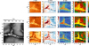 |
Fig. 1. Left: continuum intensity image normalised with spatially averaged continuum intensity. It is a small patch of a larger cube used in Paper I. The inner black box indicates the actual area used for analysis in this paper. The area outside of this box has been neglected because of the minor uncertainties in the intensity profiles that can result from the non-periodic boundary conditions. The five representative spatial points are marked. For positions 1, 3, and 5, the locations used for them in Paper I are indicated by white squares. Right: maps of the temperature (T), LOS velocity (vLOS), and magnetic field strength (B), at log(τ) = − 2.0, −0.9, and 0.0, obtained from the inversion of LTE profiles. This is used as the “reference model”. In all the 2D maps in this paper, the origin is taken as (0, 0). |
We used an Fe I atomic model with 23 levels coupled by 33 line transitions and 22 bound-free transitions. The missing UV opacity was treated using a fudge factor (Athay & Lites 1972). The other details of the model atom and profile synthesis are described in Holzreuter & Solanki (2013), and Holzreuter & Solanki (2015) and in Paper I.
2.2. Inversion of Stokes profiles
The Stokes profiles computed in LTE, 1D NLTE, and 3D NLTE were inverted in LTE using the SPINOR code (Solanki 1987; Frutiger et al. 2000). The code returns a simple atmospheric model with five parameters, temperature (T), line-of-sight velocity (vLOS), and magnetic field vector (B, γ, χ) at optical depths, log(τ) = 0.0, −0.9, and −2.0 corresponding to the chosen three inversion nodes. They were chosen based on the optimum placement discussed in Danilovic et al. (2016). The log(τ) scale was constructed at a reference wavelength of 5000 Å. Further details of the inversion can be found in Paper I.
To normalise the Stokes profiles, we used the spatially averaged continuum intensity (⟨Ic⟩). Because the 3D NLTE profiles were computed only over the sub-region, the ⟨Ic⟩ is different from the ⟨Ic⟩ that was used to normalise the LTE and 1D NLTE profiles, which were computed over the whole atmospheric cube, as described in Paper I. For a consistent comparison with the 3D NLTE profiles, we therefore repeated the inversion of LTE and 1D NLTE profiles over the sub-region using the ⟨Ic⟩ computed over that region.
3. Comparison of different atmospheres
To compare the different inverted atmospheres and to investigate the effect of NLTE and 3D RT effects on the atmospheric parameters, we used a strategy similar to that used in Paper I. We refer to the atmosphere obtained by inverting LTE profiles as the “reference model”. The atmospheres inferred from the inversion of 1D NLTE profiles and 3D NLTE profiles are referred to as “testmodel-1D” and “testmodel-3D”, respectively. The reference model was used as the fiducial model to assess the amount of change in the two testmodels. Maps of T, vLOS, B and γ at the three inversion nodes log(τ) = 0.0, −0.9 and −2.0 in the reference model are shown in Fig. 1.
The sub-region chosen for the analysis of 3D effects contains structures with a wide range of temperature, velocity, and magnetic field values, which in addition vary with height in the atmosphere. While the stronger velocity fields and magnetic fields can be determined with higher accuracy, the weak fields are quite difficult to constrain, which results in uncertainties in the inverted atmosphere. Althoug the three-node atmospheric model used here for the inversions is typical of the more complex models used to invert observations, it is an over-simplification of the complex MHD cube used for the spectral synthesis. Because there is no uniquely correct way to compare this three-node atmosphere with the actual MHD cube, there is no easy way to quantify the accuracy of either the reference or the test models against the atmosphere we used for synthesis. As discussed also in Paper I, we therefore compared the testmodels with a reference model atmosphere that was also a three-node atmosphere obtained from inversions and hence prone to the same uncertainties, except for those introduced by neglecting NLTE or 3D effects. This choice is expected to alleviate the contributions from the inversion uncertainties in our analysis. In addition, the results presented below come from a statistical study to isolate the features or locations in the atmosphere where 1D NLTE and or 3D transfer effects are expected, and to estimate how strongly they affect the inverted atmosphere. We therefore assume that any departures in testmodel-1D are purely due to 1D NLTE effects, while the deviations in the testmodel-3D are the result of a combination of 1D NLTE and 3D RT effects. In order to isolate the 3D RT effects from the 1D NLTE effects, we compared testmodel-3D with testmodel-1D. The differences between them are attributed to horizontal RT effects.
Similar to Paper I, we computed the simple and relative differences between the atmospheric models to compare each parameter. We define
 (1)
(1)
where Δx and δx represent the simple and relative differences, respectively. x is any atmospheric quantity, such as T, vLOS, B, and γ, and nD stands for either 1D or 3D. To compare the two testmodels, we use
 (2)
(2)
Because the atmospheric maps of the two test models look very similar to the reference models, we only show the difference maps in the following sections. However, the maps of all the atmospheric quantities from testmodel-1D and testmodel-3D are included in Appendix A.
After a statistical comparison of the different atmospheric models, we consider the individual features sampled by five representative spatial positions in detail. Positions 2 and 4 are identical to those used in Paper I. However, positions 1 and 3 are moved in the y-direction to bring them into the black box indicated in the continuum image in Fig. 1. This black box indicates the actual region that we used for our analysis. In all the figures, only the region within this box is displayed. The region outside of this box was neglected due to the unphysical behaviour of the intensity profiles, which is a result of the non-periodic boundary conditions. This was identified by performing two 3D calculations on different but overlapping areas in the simulation box. Relative differences between the intensities and equivalent width (EW) of the profiles in this overlapping area were compared. It was found that the effect of the non-periodic boundary is restricted to the pixels near the boundary of a computed domain. By removing the 32 rows or lines of pixels nearest to each boundary, we ensured that the effect of the boundary on the profiles was smaller than 1% everywhere. More details of this procedure are described in Holzreuter & Solanki (in prep.). The new position 1 lies closer to the edge of the granule, and position 3 lies within the same intergranular lane. Position 5 was also shifted to a region that shows stronger 3D effects, but it is still within the same magnetic structure. All the original and shifted spatial positions are marked in Fig. 1.
In Fig. 2 we compare the Stokes profiles from the LTE, 1D NLTE, and 3D NLTE runs. For clarity, we separately compare the 1D NLTE and 3D NLTE profiles in Fig. 3. The differences in their equivalent widths and residual intensities are computed using (see also Holzreuter & Solanki 2015; Smitha et al. 2020)
 (3)
(3)
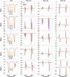 |
Fig. 2. Stokes profiles at the five representative spatial points indicated in Fig. 1. The profiles computed in LTE, 1D NLTE, and 3D NLTE are indicated in purple, black, and orange, respectively. In the first column, the differences in equivalent widths and the residual intensities with respect to the LTE profiles are indicated for the two lines. They are computed using Eq. (3). For better visibility of the differences between the profiles, we again show the 1D NLTE and 3D NLTE profiles separately in Fig. 3. |
where ILTE, InD NLTE is the minimum intensity of an LTE or nDNLTE profile at a specific spatial location, and nD stands for either 1D or 3D. The equivalent widths are represented by EWLTE, EWnD NLTE. To compare the 1D NLTE and 3D NLTE profiles in Figs. 3 and 9, we use
 (4)
(4)
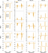 |
Fig. 3. Similar to Fig. 2, but showing a comparison between the profiles computed in 1D NLTE (black) and 3D NLTE (orange). δE′ and δI′ measure the difference in equivalent width and residual intensity between the 1D NLTE and 3D NLTE profiles. They are computed using Eq. (4). |
The LTE fit to the Stokes I and V profiles computed in 1D NLTE and 3D NLTE at the five representative positions are shown in Fig. A.3.
3.1. Temperature
A comparison of the temperatures in the reference model and the two testmodels at the three nodes is shown in Fig. 4. Although this case has been discussed in detail in Paper I, maps of the simple difference (ΔT1D) and relative difference (δT1D) of the reference model and the testmodel-1D are shown here for convenience (first and second columns). In the central and bottom nodes, the ΔT3D and δT3D maps, comparing the testmodel-3D with the reference model (third and fourth columns), are quite similar to ΔT1D and δT1D. Statistically, both testmodel-1D and testmodel-3D differ from the reference model by up to 5% in the top and central nodes. This is much lower than the 13% quoted in Paper I because we here analysed only a small sub-region of the full cube used in Paper I.
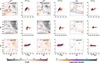 |
Fig. 4. Difference in the temperature maps from the reference model and testmodel-1D (first column), and from the reference model and testmodel-3D (third column). The fifth column shows the difference between the temperatures in testmodel-1D and testmodel-3D. The scatter density plots next to each difference image are the corresponding relative differences, defined in Eqs. (1) and (2). See Sect. 3.1 for more details. |
In the bottom node, the differences are non-zero and reach 2% (50 k–100 k), similar to what was observed in Paper I. The reason for this is that the real continuum has not been reached within the spectral window we used for the synthesis of line profiles. In addition, the information from log(τ) = 0.0 is partly transported through the NLTE opacity of the line, and thus the maps at log(τ) = 0.0 are different. Although the continuum is computed in LTE for all the three runs (LTE, 1D NLTE, and 3D NLTE), we expect to recover the same inverted temperature in the bottom node only when a significant fraction of the spectral range has true continuum in it. For the same reason, we also have non-zero ΔT3D at log(τ) = 0.0.
In Table 1 we summarize the differences between the reference model, testmodel-1D, and testmodel-3D. For each of the four parameters, T, vLOS, B and γ, we first computed the simple difference Δ defined in Eq. (1). Then we plotted a histogram for each case (not shown here, but similar histograms for the 1D NLTE case are shown in Paper I). The mean and standard deviations (S.D.) of the histogram distribution for all the four atmospheric parameters at the three inversion nodes are given in this table. The mean and S.D. provide an estimate by how much the two testmodels differ from the reference model and also from each other.
Differences of the reference model, testmodel-1D, and testmodel-3D for the four atmospheric parameters.
For the temperature, the mean and S.D. for the distribution ΔT3D computed for the testmodel-3D are lower than 100 K in all the three nodes, and they are comparable to the mean and S.D in the ΔT1D computed for the testmodel-1D. However, in the top node, the mean error in testmodel-3D increases. This means that over the sub-region considered here, the 3D effects move in the same direction as the 1D NLTE effects on average, which increases the difference to the reference model.
To isolate the 3D effects from the 1D NLTE effects, we compared testmodel-1D and testmodel-3D using Eq. (2). We list them in the last two columns of Fig. 4. In the three nodes, differences as large as 300 K are seen only in the top node. The mean of the  histogram is also the largest in this node, 21 K and 43 K, respectively (Table 1). Differences are seen in the strong magnetic element, in the intergranular lane surrounding it, and also in the granule-intergranular lane boundaries. These regions have a strong horizontal temperature gradient. In the top node,
  is positive throughout the magnetic structure (plotted in red). That is, the temperature in the testmodel-1D is higher than in testmodel-3D. This is because of the horizontal irradiation from the cooler surroundings, which makes the lines computed in 3D NLTE stronger than in 1D NLTE, as also discussed in Holzreuter & Solanki (2015). For example, the intensity profiles at position 5 plotted in Fig. 2, which lies within this magnetic structure, clearly shows this effect. At this pixel, the 3D NLTE profile is stronger than the 1D NLTE effects. δE and δI are smaller for the 3D NLTE lines than for the 1D NLTE lines, however. The 3D effects produce changes in the opposite direction to the 1D NLTE effects. Thus, at log(τ = −2.0), the temperature in testmodel-3D is closer to the reference model than in testmodel-1D, see Fig. 8.
In position 3, which is in an intergranular lane, the 3D effects weaken the intensity profiles (see Fig. 2). This is because of the irradiation from the hotter surroundings. At this pixel, the temperature in the testmodel-3D is higher than in testmodel-1D and in the reference model at log(τ) = − 2.0, see Fig. 8. This is an example of one such pixel where the 3D effects further enhance the NLTE effects and where neglecting them both introduces a combined error as large as 250 K in the temperature at the top node.
Another interesting feature, represented by position 4, is the intergranular lane immediately next to a bright magnetic structure. Hot irradiation from the magnetic structure lies one side and a granule at the other side. Accordingly, the 3D NLTE intensity profiles of the two lines are weaker than the 1D NLTE profiles. The differences in the residual intensities between the 3D NLTE and LTE runs have decreased. Testmodel-3D returns a T(log(τ) = − 2.0) value that is closer to that found by the reference model (see Fig. 8).
The temperatures at positions 1 and 2 are much less affected by 3D effects than the other three positions discussed above. At position 1, the 3D NLTE profiles are slightly weaker than the 1D NLTE profiles, whereas they are nearly the same at position 2. This can be explained by the nature of the surrounding environment, in a way similar to the other three cases discussed above.
In these five representative pixels, the 3D NLTE effects in intensity are seen to mostly affect the depth of the line profile, which results in differences in temperature in different models in the top node. In the central node,  are quite small and are observed to have significant values only in a few pixels close to the magnetic structure. The
  is mostly lower than 1%. The line wings are much less affected by the 3D effects. In the bottom node, the
  and
and  is nearly zero. The mean of the histogram distributions is also nearly zero in the central and bottom nodes.
3.2. Line-of-sight velocity
We now discuss how the LOS velocity in testmodel-3D deviates from the reference model. Based on the simple difference and relative difference maps shown in Fig. 5, the errors in the testmodel-3D are of similar magnitude as in the testmodel-1D. These errors are concentrated at the boundaries of the granules and along the intersection of the intergranular lanes and the magnetic structure. In these regions, the plasma is highly turbulent with strong velocity gradients. The 1D NLTE effects dominate the 3D effects. For a fraction of the pixels, the relative differences are large (> 50%). These come from regions of lower velocities in the MHD cube. The absolute error is more or less independent of the actual value, however. Like in Paper I, we again neglected pixels with vLOS < 10 m s−1 to avoid smaller denominators in Eq. (1). The mean and standard deviations of histograms Δv1D and Δv3D given in Table 1 are comparable, while these values for  are a few times 10 m s−1.
The measurement errors in vLOS at the five representative spatial positions in testmodel-1D and testmodel-3D (see Fig. 8) are of similar magnitude. At positions 1 and 2, velocities in testmodel-1D and testmodel-3D match the reference values closely. In the intergranular lane, at position 3, the errors are large in the testmodels at log(τ) = − 0.9 and 0.0. A Doppler shift in the line core is clearly visible in Fig. 2 at this position. The velocity at position 4 is quite interesting because in testmodel-1D its value is close to the reference value, but in testmodel-3D, the error has increased significantly at all three nodes. As discussed in Paper I, this is a point in the intergranular lane next to a magnetic structure. It is in a region of extreme gradients in flow velocities that arise because the magnetic flux sheet is tilted into the adjacent granule (see Fig. 10 of Holzreuter & Solanki 2015). In this case, the 3D effects further strengthen the 1D NLTE effects, resulting in a large deviation of the measured value in testmodel-3D. At position 5, which is inside the magnetic structure that is sandwiched between cooler environments, we observe the opposite. That is, the 3D effect has weakened the 1D NLTE effect, thus reducing the error in the measured velocity, similar to the behaviour reported for the temperature.
Holzreuter & Solanki (2013) found that the Doppler shifts in the 1D NLTE profiles differ from the 3D NLTE profiles by only about 100 m s−1. When we compare the velocity maps from the two test models (last two columns in Fig. 5), the overall 3D effects on the velocity determination are quite small. 3D RT effects are mostly observed at the boundaries of intergranular lanes and magnetic structures, which also happen to be the regions of strong 1D NLTE effects. The histograms of the  maps peak at zero in all three nodes with a standard deviation below 40 m s−1.
3.3. Magnetic field
Based on the calculations in a flux tube model, Stenholm & Stenflo (1978) noted that multi-dimensional RT effects can affect the magnetic field measurements. This was further corroborated by the findings of Holzreuter & Solanki (2012). We find this to be true also in an MHD cube. However, the general properties of the difference maps ΔB1D and ΔB3D are statistically similar, as in the case of temperature and velocity measurements. This is the case also for the magnetic field inclination and its difference maps plotted in Fig. 7. Figure 6 shows that the relative difference δB3D is as high as 50% or more for lower values of BLTE < 300 G, similar to δB1D. In most of the pixels, however, the relative difference is within 20%. The errors in testmodel-3D are smaller in the central node as it is best constrained in the inversions. A part of the errors at log(τ) = 0 is due to the difficulties in measuring small-scale weak fields close to the surface (note the larger noise in the panels in last rows of Figs. 6 and 7). However, the clear structure at log(τ) = 0.0 in the difference between testmodels 1D and 3D, just as for other nodes, suggests that these could be due to 1D NLTE and horizontal transfer effects.
When we focus on the 3D effects in particular, differences between testmodel-1D and testmodel-3D are larger in the top and bottom nodes, and much smaller in the central node. In the top node, the 3D effects are visible in pixels throughout the magnetic structure and in a patch at the upper left, which is at the intersection of a granule, an intergranular lane, and a magnetic structure. The polarisation profiles show variations due to 3D effects in this region (not shown in the paper), and this affects the inverted field strength. In addition, because the plasma within this small junction has different temperatures, we expect the horizontal irradiation to affect the equivalent widths of the lines and thus affect the magnetic field strength. The 3D effects in this region are also detected in the derived temperature maps of Fig. 4. The  maps in the top node suggest that the overall field strength in testmodel-3D is lower than in testmodel-1D.
When we consider the individual profiles, the 3D effects are seen to not only affect the intensity but also the polarisation, even if to a much lower extent. When the polarisation signals are weak, isolating the effects of 3D RT from the uncertainties in the inversions becomes difficult. Stenholm & Stenflo (1978) and Holzreuter & Solanki (2012) found that the 3D RT effects weaken the Q/Ic and V/Ic profiles. Of all the five positions in our selection, the V profiles at position 1 show noticeable weakening by 3D effects. Although small differences in the 3D NLTE case are also seen in linear polarisation, the profiles are quite weak (< 1%). When we examine the inclination maps in the reference model around position 1 (Fig. 1), the inclination changes quite drastically. This can contribute to the horizontal transfer effects in the polarisation profiles. The differences are as large as 50° between the inclinations found in testmodel-1D and testmodel-3D at position 1 and the region surrounding it, at all the three nodes (Figs. 7 and 8). Because such a large difference is not specific to one isolated pixel but is observed over an extended region following the boundary between the granule-intergranular lane, it is possible that the horizontal transfer effects play a role. In particular, the 3D effects at this position have shifted the measured inclination farther away from the reference value.
At position 5, the exact opposite is observed as all the Stokes profiles, I/Ic, Q/Ic, U/Ic, and V/Ic, show strengthening from the 3D effects. This supports the findings of Holzreuter & Solanki (2015) that the horizontal RT strengthens the line at the centres of magnetic elements. The effect is especially clear in the 6301.5 Å line. In the second line at 6302.5 Å, the 3D effects weaken the π components and strengthen the blue σ components in the Q/Ic and U/Ic profiles. This is because regions with different temperatures surround position 5. The magnetic field strength at log(τ) = − 2.0 in testmodel-3D has shifted closer to the reference value, but away from it in the bottom node.
At the other three positions, positions 2, 3, and 4, the polarisation profiles computed in 3D NLTE are slightly weaker than the 1D NLTE profiles (Fig. 3). The errors due to neglecting 3D effects are enhanced at some nodes and reduced in others (Fig. 8).
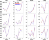 |
Fig. 8. Values of the different atmospheric quantities in the reference model (black), in testmodel-1D (red), and in testmodel-3D (blue) at the five representative spatial positions at all three inversion nodes. |
4. Effects of spatial and spectral degradation
In Paper I we showed that the 1D NLTE effects in the Stokes profiles survive even when they are spatially averaged. We here conducted a similar test to confirm the strength of 3D NLTE effects when the Stokes profiles are degraded both spatially and spectrally. For this, we considered the specifications of the CRisp Imaging SpectroPolarimeter (CRISP, Scharmer et al. 2008) at the Swedish Solar Telescope (SST, Scharmer et al. 2003). The data were degraded to a spectral resolution of 60 mÅ and a spatial resolution of 0.1″. The spectral and spatial point spread functions (PSF) were assumed to be Gaussian. In addition, we added Gaussian noise with a standard deviation of 1 × 10⁻³Ic. The inversions were made in a similar way as in the case without any degradation (Sect. 2.2).
Figure 9 shows the effects of spectral smearing and noise on the Stokes profiles from Fig. 3. Because their signals are weak, the polarisation profiles are more affected by this spectral degradation than the intensity profiles. The differences between the 1D NLTE and 3D NLTE profiles, although small in the non-degraded case, are still observed after spectral smearing and wavelength rebinning. The values of δE′ and δI′, computed using Eq. (4), are close to the values measured for the original profiles. In a few cases such as at positions 1 and 2, spectral degradation has reduced δI′1 by a small amount.
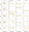 |
Fig. 9. Effects of spectral degradation and noise on the Stokes profiles computed in 1D NLTE (black) and 3D NLTE (orange) at the five spatial positions. The differences in equivalent widths δE′ and residual intensities δI′ are computed using Eq. (4). See Sect. 4 for more details. |
The temperature in the atmospheric models obtained by the inversion of spatially and spectrally degraded profiles is compared in Fig. 10. Figures 10 and 4 are similar in the simple difference and in relative difference maps. While in some regions, the spatial and spectral degradation has reduced the 3D NLTE effects, in some other regions, the differences are much larger than before. This might be a result of spatial binning. This is because this effect was also seen in Paper I (see Fig. 12 of that paper) where the profiles were only spatially binned and no other degradation was applied. The spatial smearing and noise can also further enhance this effect. The LOS velocity and magnetic field maps shown in Appendix B also show a similar behaviour.
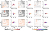 |
Fig. 10. Same as Fig. 4, but for the Stokes profiles degraded to the specifications of the CRISP instrument on the Swedish Solar Telescope. See Sect. 4 for more details. |
We repeated this test by degrading the data to the specifications of the Visible Spectro-Polarimeter (ViSP, Elmore et al. 2014) at the Daniel K. Inouye Solar Telescope (DKIST). Because the ViSP observes at a much higher resolution that the CRISP, the effects of 1D NLTE and horizontal transfer were seen at almost the same level as in the original simulation.
5. Summary and conclusions
In continuation to Paper I, we studied the errors introduced in the inverted model atmosphere when 3D RT effects are neglected. We selected a small region of the large MHD cube used in Paper I to perform the 3D NLTE computations and then inverted the profiles using the LTE inversion code SPINOR. The derived atmosphere, called testmodel-3D, was then compared with the reference model obtained from the inversion of LTE profiles. Any departure between the two was attributed to 3D NLTE effects. In addition to this, we also compared the atmospheric model from the inversion of 1D NLTE profiles called testmodel-1D in the same region. Testmodel-1D and testmodel-3D were compared to isolate the 3D RT effects.
Holzreuter & Solanki (2013), and Holzreuter & Solanki (2015) nicely summarised that the 3D effects weaken the lines when there is horizontal irradiation from hotter surroundings, and the effects strengthen the line profile when the surroundings are cooler. The derived quantities in such regions differ in testmodel-3D compared to testmodel-1D. This is observed along the boundaries of magnetic structures and their surrounding intergranular lanes, granule-intergranular lane boundaries, and in pixels inside magnetic structures that are affected by irradiation from cool intergranular lanes. Because the 3D effects can weaken or strengthen the 1D NLTE line profiles, they can either enhance or reduce the departure from the reference model.
Figure 11 demonstrates the location in the sub-region of the cube in which the 3D effects enhance or weaken the 1D NLTE effects. Pixels in black highlight the regions where 3D effects enhance 1D NLTE effects, that is, the values in testmodel-3D are shifted farther away from the reference model than those in testmodel-1D. Regions highlighted in white show the opposite effect. In these regions, the 3D effects weakens the 1D NLTE effects. Regions in grey represent pixels where the 3D effects are weak and so do not fall into either of the two categories. The threshold values for dividing the pixels into these three categories are 50 K, 100 m s−1, 100 G, and 10° in T, vLOs, B, and γ, respectively.
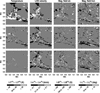 |
Fig. 11. Patches representing the regions where horizontal RT enhances the NLTE effects (white), weaken the NLTE effects (black), or has no significant influence (grey). From left to right, we show this for T, vLOS, B, and γ at all the three inversion nodes; from top to bottom log(τ) = − 2.0, −0.9, and 0.0. The threshold values employed to divide the regions into the three categories are indicated in the colour bar. See Sect. 5 for further details. |
This figure shows that the 3D effects are most prominent in and around the magnetic structure, and they clearly affect the temperature and velocity measurements. Because the 3D effects mostly affect the line core, we see their effect more clearly in the top node. In the regions that are affected (black and white patches), the departures range between 50 K–100 K.
In velocity maps, 3D effects can alter the values between 100 m s−1–500 m s−1. Some effects are also observed in the central and bottom nodes, in regions of strong velocity gradients, such as at position 4, which we showed in Sect. 3.2 and discussed in Paper I. These gradients are difficult to recover in the simple three-node atmospheric model we used.
In the case of magnetic field strength and inclination, the white and black patches are scattered throughout the sub-region. The errors in the magnetic field strength caused by neglecting 3D effects is in the range 100 G–500 G, and in inclination, the errors are between 10°–50°. 3D effects are significant in the measured magnetic field inclination in a patch below a magnetic structure, as discussed in Sect. 3.3. Only in this patch are the errors larger than 50° in a few pixels.
To conclude, the errors introduced in the inverted atmosphere by neglecting 3D RT effects are not as large as the errors when NLTE effects are neglected completely, at least in the sub-region analysed here. The 3D effects are more localised in regions surrounded by strong horizontal gradients in temperature and intensity, such as magnetic flux concentrations (Carlsson et al. 2004). Neglecting their effects not only introduces errors in temperature determination, but to a lesser extent, also in other parameters. In Sect. 4 we have tested how the spatial and spectral degradation of the Stokes profiles in the presence of noise affects the 1D NLTE and horizontal RT effects. The difference maps comparing the reference and testmodels are similar as in the case without degradation. This demonstrates that even at low spectral and spatial resolutions, the statistical nature of the errors introduced in the inverted atmosphere by neglecting 1D NLTE and/or 3D effects can remain the same.
The 3D effects can be expected at granular boundaries, intergranular lanes, and magnetic bright points. In the construction of atmospheric models for photospheric bright points (e.g., Shelyag et al. 2010; Hewitt et al. 2014), the 3D effects are neglected although they can affect the temperature stratification. Based on the results of this study, we expect that the 3DRT effects are also important in other photospheric features such as sunspots, where we observe horizontal gradients in temperatures across the umbra-penumbra boundaries, penumbral filaments and spines, boundaries of light bridges, and umbral dots. The atmospheric diagnostics of these features (Socas-Navarro et al. 2004; Riethmüller et al. 2008; Tiwari et al. 2013, 2015) carried out by neglecting 3D effects can result in errors in the deduced quantities.
No inversion codes are currently capable of performing 3D NLTE calculations because it requires large computational resources. However, it is important to consider the errors that can be introduced in the inverted atmosphere when 3D RT effects are neglected.
Acknowledgments
We thank the anonymous referee for constructive comments which helped improve the paper. This project has received funding from the European Research Council (ERC) under the European Union’s Horizon 2020 research and innovation programme (Grant agreement No. 695075). This work has also been partially supported by the BK21 plus program through the National Research Foundation (NRF) funded by the Ministry of Education of Korea. This research has made use of NASA’s Astrophysics Data System.
References
- Anusha, L. S., & Nagendra, K. N. 2013, ApJ, 767, 108 [Google Scholar]
- Asplund, M., Carlsson, M., & Botnen, A. V. 2003, A&A, 399, L31 [NASA ADS] [CrossRef] [EDP Sciences] [Google Scholar]
- Asplund, M., Grevesse, N., Sauval, A. J., Allende Prieto, C., & Kiselman, D. 2004, A&A, 417, 751 [NASA ADS] [CrossRef] [EDP Sciences] [Google Scholar]
- Asplund, M., Grevesse, N., Sauval, A. J., Allende Prieto, C., & Kiselman, D. 2005, A&A, 435, 339 [NASA ADS] [CrossRef] [EDP Sciences] [Google Scholar]
- Athay, R. G., & Lites, B. W. 1972, ApJ, 176, 809 [Google Scholar]
- Avery, L. W., & House, L. L. 1969, Sol. Phys., 10, 88 [Google Scholar]
- Avrett, E. H., & Loeser, R. 1971, J. Quant. Spectr. Rad. Transf., 11, 559 [Google Scholar]
- Bergemann, M., Gallagher, A. J., Eitner, P., et al. 2019, A&A, 631, A80 [NASA ADS] [CrossRef] [EDP Sciences] [Google Scholar]
- Bjørgen, J. P., Sukhorukov, A. V., Leenaarts, J., et al. 2018, A&A, 611, A62 [NASA ADS] [CrossRef] [EDP Sciences] [Google Scholar]
- Cannon, C. J. 1970, ApJ, 161, 255 [Google Scholar]
- Cannon, C. J. 1971, Sol. Phys., 21, 82 [Google Scholar]
- Cannon, C. J., & Rees, D. E. 1971, ApJ, 169, 157 [Google Scholar]
- Carlsson, M. 2008, Phys. Scr., 133, 014012 [Google Scholar]
- Carlsson, M., Stein, R. F., Nordlund, Å., & Scharmer, G. B. 2004, ApJ, 610, L137 [Google Scholar]
- Danilovic, S., van Noort, M., & Rempel, M. 2016, A&A, 593, A93 [NASA ADS] [CrossRef] [EDP Sciences] [Google Scholar]
- Elmore, D. F., Rimmele, T. R., Casini, R., et al. 2014, Proc SPIE, 9147, 914707 [Google Scholar]
- Frutiger, C., Solanki, S. K., Fligge, M., & Bruls, J. H. M. J. 2000, A&A, 358, 1109 [NASA ADS] [Google Scholar]
- Gallagher, A. J., Bergemann, M., Collet, R., et al. 2020, A&A, 634, A55 [NASA ADS] [CrossRef] [EDP Sciences] [Google Scholar]
- Hewitt, R. L., Shelyag, S., Mathioudakis, M., & Keenan, F. P. 2014, A&A, 565, A84 [Google Scholar]
- Holzreuter, R., & Solanki, S. K. 2012, A&A, 547, A46 [NASA ADS] [CrossRef] [EDP Sciences] [Google Scholar]
- Holzreuter, R., & Solanki, S. K. 2013, A&A, 558, A20 [NASA ADS] [CrossRef] [EDP Sciences] [Google Scholar]
- Holzreuter, R., & Solanki, S. K. 2015, A&A, 582, A101 [NASA ADS] [CrossRef] [EDP Sciences] [Google Scholar]
- Kiselman, D., & Nordlund, A. 1995, A&A, 302, 578 [Google Scholar]
- Leenaarts, J., Carlsson, M., Hansteen, V., & Rouppe van der Voort, L. 2009, ApJ, 694, L128 [Google Scholar]
- Leenaarts, J., Rutten, R. J., Reardon, K., Carlsson, M., & Hansteen, V. 2010, ApJ, 709, 1362 [Google Scholar]
- Leenaarts, J., Carlsson, M., & Rouppe van der Voort, L. 2012, ApJ, 749, 136 [Google Scholar]
- Leenaarts, J., Pereira, T. M. D., Carlsson, M., Uitenbroek, H., & De Pontieu, B. 2013, ApJ, 772, 90 [Google Scholar]
- Leenaarts, J., Carlsson, M., & Rouppe van der Voort, L. 2015, ApJ, 802, 136 [Google Scholar]
- Lind, K., Amarsi, A. M., Asplund, M., et al. 2017, MNRAS, 468, 4311 [Google Scholar]
- Nordlund, A. 1985, in NATO Advanced Science Institutes (ASI) Series C, eds. J. E. Beckman, & L. Crivellari, NATO ASI Ser. C, 152, 215 [Google Scholar]
- Pereira, T. M. D., Asplund, M., & Kiselman, D. 2009, A&A, 508, 1403 [NASA ADS] [CrossRef] [EDP Sciences] [Google Scholar]
- Prakapavičius, D., Steffen, M., Kučinskas, A., et al. 2013, Mem. Soc. Astron. it. Supp., 24, 111 [Google Scholar]
- Riethmüller, T. L., Solanki, S. K., & Lagg, A. 2008, ApJ, 678, L157 [NASA ADS] [CrossRef] [Google Scholar]
- Rutten, R. J. 1988, in IAU Colloq. 94, eds. R. Viotti, A. Vittone, & M. Friedjung, Astrophys. Space Sci. Lib., 138, 185 [Google Scholar]
- Rutten, R. J., & Kostik, R. I. 1982, A&A, 115, 104 [NASA ADS] [Google Scholar]
- Scharmer, G. B., Bjelksjo, K., Korhonen, T. K., Lindberg, B., & Petterson, B. 2003, in Innovative Telescopes and Instrumentation for Solar Astrophysics, eds. S. L. Keil, & S. V. Avakyan, SPIE Conf. Ser., 4853, 341 [Google Scholar]
- Scharmer, G. B., Narayan, G., Hillberg, T., et al. 2008, ApJ, 689, L69 [Google Scholar]
- Shchukina, N., & Trujillo Bueno, J. 2001, ApJ, 550, 970 [Google Scholar]
- Shelyag, S., Mathioudakis, M., Keenan, F. P., & Jess, D. B. 2010, A&A, 515, A107 [NASA ADS] [CrossRef] [EDP Sciences] [Google Scholar]
- Smitha, H. N., Holzreuter, R., van Noort, M., & Solanki, S. K. 2020, A&A, 633, A157 [NASA ADS] [CrossRef] [EDP Sciences] [Google Scholar]
- Socas-Navarro, H., Pillet, V. M., Sobotka, M., & Vazquez, M. 2004, ApJ, 614, 448 [Google Scholar]
- Solanki, S. K. 1987, PhD Thesis, ETH, Zürich [Google Scholar]
- Solanki, S. K., & Steenbock, W. 1988, A&A, 189, 243 [NASA ADS] [Google Scholar]
- Steffen, M., Prakapavičius, D., Caffau, E., et al. 2015, A&A, 583, A57 [NASA ADS] [CrossRef] [EDP Sciences] [Google Scholar]
- Stenholm, L. G. 1977, A&A, 54, 577 [NASA ADS] [Google Scholar]
- Stenholm, L. G., & Stenflo, J. O. 1977, A&A, 58, 273 [NASA ADS] [Google Scholar]
- Stenholm, L. G., & Stenflo, J. O. 1978, A&A, 67, 33 [NASA ADS] [Google Scholar]
- Sukhorukov, A. V., & Leenaarts, J. 2017, A&A, 597, A46 [NASA ADS] [CrossRef] [EDP Sciences] [Google Scholar]
- Tiwari, S. K., van Noort, M., Lagg, A., & Solanki, S. K. 2013, A&A, 557, A25 [NASA ADS] [CrossRef] [EDP Sciences] [Google Scholar]
- Tiwari, S. K., van Noort, M., Solanki, S. K., & Lagg, A. 2015, A&A, 583, A119 [NASA ADS] [CrossRef] [EDP Sciences] [Google Scholar]
- Uitenbroek, H. 2001, ApJ, 557, 389 [NASA ADS] [CrossRef] [Google Scholar]
- Vögler, A., Shelyag, S., Schüssler, M., et al. 2005, A&A, 429, 335 [NASA ADS] [CrossRef] [EDP Sciences] [Google Scholar]
Appendix A: Testmodels and fit to the Stokes profiles
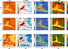 |
Fig. A.1. Maps of different atmospheric quantities in testmodel-1D. |
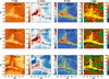 |
Fig. A.2. Maps of different atmospheric quantities in testmodel-3D. |
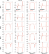 |
Fig. A.3. LTE fit to the Stokes profiles shown in Fig. 3. The input profiles are computed in 1D NLTE (first two columns) and in 3D NLTE (last two columns). |
Appendix B: Effects of spatial and spectral degradation on the velocity and magnetic field measurements
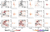 |
Fig. B.1. Same as Fig. 5, but for the Stokes profiles degraded to the specifications of the CRISP instrument on the Swedish Solar Telescope. See Sect. 4 for more details. |
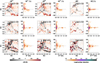 |
Fig. B.2. Same as Fig. 6, but for the Stokes profiles degraded to the specifications of the CRISP instrument on the Swedish Solar Telescope. See Sect. 4 for more details. |
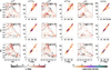 |
Fig. B.3. Same as Fig. 7, but for the Stokes profiles degraded to the specifications of the CRISP instrument on the Swedish Solar Telescope. See Sect. 4 for more details. |
All Tables
Differences of the reference model, testmodel-1D, and testmodel-3D for the four atmospheric parameters.
All Figures
|
Fig. 1. Left: continuum intensity image normalised with spatially averaged continuum intensity. It is a small patch of a larger cube used in Paper I. The inner black box indicates the actual area used for analysis in this paper. The area outside of this box has been neglected because of the minor uncertainties in the intensity profiles that can result from the non-periodic boundary conditions. The five representative spatial points are marked. For positions 1, 3, and 5, the locations used for them in Paper I are indicated by white squares. Right: maps of the temperature (T), LOS velocity (vLOS), and magnetic field strength (B), at log(τ) = − 2.0, −0.9, and 0.0, obtained from the inversion of LTE profiles. This is used as the “reference model”. In all the 2D maps in this paper, the origin is taken as (0, 0). |
| In the text | |
|
Fig. 2. Stokes profiles at the five representative spatial points indicated in Fig. 1. The profiles computed in LTE, 1D NLTE, and 3D NLTE are indicated in purple, black, and orange, respectively. In the first column, the differences in equivalent widths and the residual intensities with respect to the LTE profiles are indicated for the two lines. They are computed using Eq. (3). For better visibility of the differences between the profiles, we again show the 1D NLTE and 3D NLTE profiles separately in Fig. 3. |
| In the text | |
|
Fig. 3. Similar to Fig. 2, but showing a comparison between the profiles computed in 1D NLTE (black) and 3D NLTE (orange). δE′ and δI′ measure the difference in equivalent width and residual intensity between the 1D NLTE and 3D NLTE profiles. They are computed using Eq. (4). |
| In the text | |
|
Fig. 4. Difference in the temperature maps from the reference model and testmodel-1D (first column), and from the reference model and testmodel-3D (third column). The fifth column shows the difference between the temperatures in testmodel-1D and testmodel-3D. The scatter density plots next to each difference image are the corresponding relative differences, defined in Eqs. (1) and (2). See Sect. 3.1 for more details. |
| In the text | |
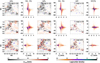 |
Fig. 5. Same as Fig. 4, but for the line-of-sight velocity. See Sect. 3.2 for further details. |
| In the text | |
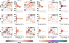 |
Fig. 6. Same as Fig. 4, but for the magnetic field strength. See Sect. 3.3 for more details. |
| In the text | |
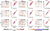 |
Fig. 7. Same as Fig. 4, but for the magnetic field inclination. See Sect. 3.3 for more details. |
| In the text | |
|
Fig. 8. Values of the different atmospheric quantities in the reference model (black), in testmodel-1D (red), and in testmodel-3D (blue) at the five representative spatial positions at all three inversion nodes. |
| In the text | |
|
Fig. 9. Effects of spectral degradation and noise on the Stokes profiles computed in 1D NLTE (black) and 3D NLTE (orange) at the five spatial positions. The differences in equivalent widths δE′ and residual intensities δI′ are computed using Eq. (4). See Sect. 4 for more details. |
| In the text | |
|
Fig. 10. Same as Fig. 4, but for the Stokes profiles degraded to the specifications of the CRISP instrument on the Swedish Solar Telescope. See Sect. 4 for more details. |
| In the text | |
|
Fig. 11. Patches representing the regions where horizontal RT enhances the NLTE effects (white), weaken the NLTE effects (black), or has no significant influence (grey). From left to right, we show this for T, vLOS, B, and γ at all the three inversion nodes; from top to bottom log(τ) = − 2.0, −0.9, and 0.0. The threshold values employed to divide the regions into the three categories are indicated in the colour bar. See Sect. 5 for further details. |
| In the text | |
|
Fig. A.1. Maps of different atmospheric quantities in testmodel-1D. |
| In the text | |
|
Fig. A.2. Maps of different atmospheric quantities in testmodel-3D. |
| In the text | |
|
Fig. A.3. LTE fit to the Stokes profiles shown in Fig. 3. The input profiles are computed in 1D NLTE (first two columns) and in 3D NLTE (last two columns). |
| In the text | |
|
Fig. B.1. Same as Fig. 5, but for the Stokes profiles degraded to the specifications of the CRISP instrument on the Swedish Solar Telescope. See Sect. 4 for more details. |
| In the text | |
|
Fig. B.2. Same as Fig. 6, but for the Stokes profiles degraded to the specifications of the CRISP instrument on the Swedish Solar Telescope. See Sect. 4 for more details. |
| In the text | |
|
Fig. B.3. Same as Fig. 7, but for the Stokes profiles degraded to the specifications of the CRISP instrument on the Swedish Solar Telescope. See Sect. 4 for more details. |
| In the text | |
Current usage metrics show cumulative count of Article Views (full-text article views including HTML views, PDF and ePub downloads, according to the available data) and Abstracts Views on Vision4Press platform.
Data correspond to usage on the plateform after 2015. The current usage metrics is available 48-96 hours after online publication and is updated daily on week days.
Initial download of the metrics may take a while.