© ESO 2021

1. Introduction

The emergence of a wind around stars is a remarkable and somewhat counter-intuitive phenomenon. The existence of the solar wind was already suggested because the tails of comets always point away from the Sun (Biermann 1951). Nevertheless, the wind was thought to be a relatively slow phenomenon associated with evaporation of the corona (Chamberlain 1960). The physical nature and mathematical theory of the solar wind was first understood by Parker (1958). His theory showed that the wind starts off as a subsonic flow some distance above the corona. It gradually gains in speed as the gravitational force diminishes and the effective outward pull resulting from the quadratic increase of the cross-sectional area in Bernoulli’s law becomes dominant. This is a purely hydrodynamic phenomenon, unlike what was suggested by the popular notion of the solar corpuscular radiation at the time.

Stellar winds play a crucial role in a star’s life. Without the wind, the Sun would still be spinning rapidly and magnetically superactive. A proper understanding of the rotational evolution of a star through magnetic braking via a wind is important not only for stellar evolution, but it also plays a role in understanding the diversity of magnetic activity as a function of the rotation rate and age (van Saders et al. 2016). As the star reaches the age of the Sun, the magnetic field either changes its geometry such that stellar braking is reduced (Metcalfe & van Saders 2017; See et al. 2019) or it can continue to brake and the star’s differential rotation becomes antisolar-like (Gastine et al. 2014; Käpylä et al. 2014), that is, the equator spins slower than the poles. Stellar winds can also be important for the dynamo itself in that they can transport magnetic helicity away from the dynamo region, and thereby alleviate what is known as catastrophic quenching; see Mitra et al. (2011) for mean-field models and Del Sordo et al. (2013) for computations of the magnetic helicity flux in simulations in a turbulent wind. Magnetic winds also affect the density and dynamics of cosmic rays in the heliosphere. Selfconsistently computing the dynamo-generated magnetic field evolution in the heliosphere is, therefore, also crucial for modeling the magnetic shielding of Galactic cosmic rays on Earth.

The theory of a magnetized stellar wind by Weber & Davis (1967) employed a prescribed and time-independent stellar magnetic field, so any feedback on the underlying dynamics was ignored. This is also true of the recent numerical models of Réville et al. (2015), who compared different magnetic multipoles as initial conditions of their models. This has changed only in recent years. Given that the wind normally dominates over the magnetic field, one can separate the dynamics of the wind from that of the solar dynamo. Pinto et al. (2011), and more recently Perri et al. (2018), modeled this by using two separate codes that are magnetically coupled through a matching condition at the solar surface. In more recent work, Perri et al. (2020) extended their model to also include a mean-field dynamo solution in the Pluto code, rather than matching the solutions of two separate codes. This allows for feedback from the wind onto the dynamo. This is therefore similar to the work presented here, except that they still invoke what they call a multilayered boundary condition. This means that different equations are being solved inside and outside the star. The model is therefore still not fully self-consistent, but in some ways more realistic than ours.

The purpose of the present paper is to explore some basic properties of stellar winds in the presence of dynamo-generated magnetic fields. It is appropriate to adopt a mean-field model, where we solve the equations for the azimuthally averaged magnetic and velocity fields. In this paper, those mean fields are denoted by an overbar. The effects of turbulence are then parameterized through a turbulent viscosity and a turbulent magnetic diffusivity. In the star’s convection zone, there are also cyclonic convective motions giving rise to kinetic helicity of opposite signs in the two hemispheres. This is modeled through an α effect (Krause & Rädler 1980). The turbulent magnetic diffusivity is here assumed constant.

The presence of the magnetic field causes the kinetic and magnetic stresses to be different from zero. The turbulent viscosity is itself a result of kinetic and magnetic stresses caused by the fluctuating components of the magnetic and velocity fields. In the theory of turbulent accretion disks (Frank et al. 1992), those stresses are parameterized by the Shakura & Sunyaev (1973) parameter, α_SS. It quantifies the stress in terms of the background differential rotation, the sound speed, and the scale height. In accretion disks, where the differential rotation is Keplerian, this amounts to a scaling of the stress by the sound speed squared. In our case, the differential rotation is not related to the sound speed, but the basic mechanism of angular momentum transfer is the same, and we can still express the total stress in a similar fashion.

Unlike the work of Perri et al. (2018), we consider the evolution of the dynamo and the wind within a single code. At this point, our aim is not to produce a realistic model of the Sun, but rather a physically consistent model under conditions where the dynamics of the wind can no longer be separated from that of the dynamo. Our models can also be applied to conditions of rapid rotation, which strongly affects the wind. This can be particularly relevant to young stars in their T Tauri phase. We begin by presenting the basic equations of our model and turn then to the discussion of our results.

The simplest wind solution is the isothermal one that was already found by Parker (1958). Heating is not explicitly invoked. Its physics resembles that of a siphon flow. Once a fluid parcel has moved over the top of the effective gravitational potential, it simply continues to fall and pulls the remaining fluid behind it (Shore 1992). The top of the effective potential corresponds to the critical point where the flow speed crosses the sonic point. We arrange this point to be in the middle of the computational domain such that the flow speed becomes supersonic well before the outer point r_out. We fit the dynamo-active zone (or stellar envelope) with an α effect different from zero into a spherical shell between the inner point of the computational domain, r_in, and a radius R, which models the surface of the star.

The usefulness of an isothermal solution can be justified by considering the fact that the sound speed both at the bottom of the convection zone and in the solar wind is about 100 km s⁻¹, corresponding to a temperature of a million degrees. The lower temperature near the photosphere is obviously ignored. For an isothermal gas, the mean pressure $\overline{p}$ is then simply proportional to the gas density $\overline{\rho }$ with $\overline{p}=\overline{\rho }{c_{\text{s}}}^2$, where c_s is the isothermal sound speed. The pressure gradient is then given by $(\mathbf{\nabla }\overline{p})/\overline{\rho }={c_{\text{s}}}^2\mathbf{\nabla }ln\overline{\rho }$. The implications of a cool photosphere will be discussed at the end of the paper.

We begin by discussing first the basic equations, boundary conditions, and parameters in Sect. 2. We then present our results in Sect. 3, and draw our conclusions in Sect. 4.

2. The model

We adopt spherical polar coordinates, (r, θ, ϕ), with the origin at the center of the star. The vector r points away from the center, the colatitude θ increases away from the north pole, and ϕ increases in the eastward direction. We assume axisymmetry, that is, ∂/∂ϕ = 0.

2.1. Basic equations

We write the mean magnetic field as $\overline{\mathit{B}}=\mathbf{\nabla }\times \overline{\mathit{A}}$, where $\overline{\mathit{A}}$ is the mean vector potential. This ensures that $\mathbf{\nabla }·\overline{\mathit{B}}=0$ at all times. The evolution equations for $\overline{\mathit{A}}$, the mean velocity $\overline{\mathit{U}}$, and the logarithmic mean density $\overline{\rho }$, are

$$\begin{array}{cc}& \frac{\partial \overline{\mathit{A}}}{\partial t}=\overline{\mathit{U}}\times \overline{\mathit{B}}+\alpha \overline{\mathit{B}}-{\eta }_{\mathrm{T}}{\mu }_0\overline{\mathit{J}},\hfill \end{array}$$(1)

$$\begin{array}{cc}& \frac{\mathrm{D}\overline{\mathit{U}}}{\mathrm{D}t}=-c_{\mathrm{s}}^2\mathbf{\nabla }ln\overline{\rho }-\frac{\mathit{GM}}{r^2}\widehat{\mathit{r}}+\frac{1}{\overline{\rho }}\overline{\mathit{J}}\times \overline{\mathit{B}}-{\nu }_{\mathrm{T}}\overline{\mathcal{Q}},\hfill \end{array}$$(2)

$$\begin{array}{cc}& \frac{\mathrm{D}ln\overline{\rho }}{\mathrm{D}t}=-\mathbf{\nabla }·\overline{\mathit{U}},\hfill \end{array}$$(3)

where $\text{D}/\text{D}t=\partial /\partial t+\overline{\mathit{U}}·\mathbf{\nabla }$ is the advective derivative, G is Newton’s constant, M is the stellar mass, $\widehat{\mathit{r}}=\mathit{r}/r$ is the radial unit vector, η_T and ν_T are the sums of turbulent and microphysical values of magnetic diffusivity and kinematic viscosity, respectively, α is the aforementioned coefficient in the α effect, $\overline{\mathit{J}}=\mathbf{\nabla }\times \overline{\mathit{B}}/{\mu }_0$ is the mean current density, μ₀ is the vacuum permeability,

$$\begin{array}{c}\hfill -\overline{\mathcal{Q}}={\mathrm{\nabla }}^2\overline{\mathit{U}}+\frac{1}{3}\mathbf{\nabla }\mathbf{\nabla }·\overline{\mathit{U}}+2\overline{\mathbf{S}}·\mathbf{\nabla }ln({\nu }_{\mathrm{T}}\overline{\rho })\end{array}$$(4)

is a term appearing in the viscous force, where $\overline{\mathbf{S}}$ is the traceless rate of strain tensor of the mean flow with components ${\overline{\mathsf{S}}}_{\mathit{ij}}=\frac{1}{2}({\overline{U}}_{i,j}+{\overline{U}}_{j,i})-\frac{1}{3}{\delta }_{\mathit{ij}}\mathbf{\nabla }·\overline{\mathit{U}}$. The dot in Eq. (4) denotes the contraction over the free index of $\mathbf{\nabla }ln({\nu }_{\text{T}}\overline{\rho })$.

The mean magnetic field is generated by the α effect. This leads to exponential growth, provided the value of α is above a certain critical value. Eventually, the dynamo must saturate because the Lorentz force from the mean field, $\overline{\mathit{J}}\times \overline{\mathit{B}}$, drives fluid motions that feed back onto the dynamo to limit its growth. This way of achieving saturation is sometimes referred to as Malkus & Proctor (1975) mechanism. In addition, there can be feedback from the small-scale magnetic field that leads to a nonlinear suppression of α, which is referred to as α quenching. We assume here a simple quenching function for α, which is then written in the form

$$\begin{array}{c}\hfill \alpha (r,\theta ,\overline{\mathit{B}})=\frac{{\alpha }_0{f}_{\alpha }(r)cos\theta {sin}^n\theta }{1+Q_{\alpha }{\overline{\mathit{B}}}^2/B_{\mathrm{eq}}^2},\end{array}$$(5)

where n = 6 is chosen to concentrate the α effect to low latitudes (Jabbari et al. 2015; Cole et al. 2016), Q_α is a quenching parameter that determines the typical field strength, which is expected to be on the order of $Q_{\alpha }^{-1/2}{B}_{\text{eq}}$, and

$$\begin{array}{c}\hfill f_{\alpha }(r)=\mathrm{\Theta }((r-R)/w_{\alpha })\end{array}$$(6)

is a radial profile function with Θ(x) being a smoothened step function from 0 to 1 as x crosses zero. Here, R and w_α determine the location and width of the transition. The value of Q_α determines the nonlinear equilibration of the dynamo, in addition to the macroscopic feedback from the Lorentz force mentioned above. Our model thus comprises three distinct layers with

$$\begin{array}{c}\hfill r_{\mathrm{in}}<R<r_{\mathrm{c}}<r_{\mathrm{out}},\end{array}$$(7)

where r_in < r < R is the dynamo region (modeling the stellar envelope), R < r < r_c is the wind acceleration region (modeling the locations of the solar corona and the Alfvén point), and r_c < r < r_out is the supersonic wind region with $r_{\text{c}}=GM/2c_{\text{s}}{}^2$ being the critical point.

2.2. Boundary conditions

In most of the cases, we apply a uniform angular velocity Ω₀ on the inner boundary r = r_in by setting u_ϕ = r_insinθ Ω₀. For the other two velocity components, we adopt “open” boundary conditions by setting the second radial derivative to zero. This condition turns out to be stable in all cases considered in this paper. It allows for a weak inflow to replenish the mass loss on the outer boundary r = r_out, where we apply open boundary conditions for all three velocity components. No precautions are taken to ensure that the mass in the computational domain stays constant. It turns out, however, that the total mass remains nearly unchanged. This is, to some extent, also explained by the fact that the total mass loss rate is small compared with other inverse time scales in the problem.

For the magnetic field, we adopt a perfect conductor boundary condition on the inner radius, that is,

$$\begin{array}{c}\hfill \frac{\partial {\overline{A}}_r}{\partial r}={\overline{A}}_{\theta }={\overline{A}}_{\varphi }=0\mathrm{on}r=r_{\mathrm{in}},\end{array}$$(8)

and a radial field condition on the outer radius, that is,

$$\begin{array}{c}\hfill {\overline{A}}_r=\frac{\partial {\overline{A}}_{\theta }}{\partial r}+\frac{{\overline{A}}_{\theta }}{r}=\frac{\partial {\overline{A}}_{\varphi }}{\partial r}+\frac{{\overline{A}}_{\varphi }}{r}=0\mathrm{on}r=r_{\mathrm{out}}.\end{array}$$(9)

On the pole, we assume

$$\begin{array}{c}\hfill \frac{\partial {\overline{A}}_r}{\partial \theta }={\overline{A}}_{\theta }={\overline{A}}_{\varphi }=0\mathrm{on}\theta =0^{°},\end{array}$$(10)

while on the equator, we assume

$$\begin{array}{c}\hfill \frac{\partial {\overline{A}}_r}{\partial \theta }={\overline{A}}_{\theta }=\frac{\partial {\overline{A}}_{\varphi }}{\partial \theta }=0\mathrm{on}\theta ={90}^{°}.\end{array}$$(11)

Since our simulations are axisymmetric, the magnetic field is conveniently represented via ${\overline{B}}_{\varphi }$ and ${\overline{A}}_{\varphi }$. In particular, contours of $rsin\theta {\overline{A}}_{\varphi }$ give the magnetic field lines of the poloidal field, ${\overline{\mathit{B}}}_{\mathrm{pol}}=\mathbf{\nabla }\times ({\overline{A}}_{\varphi }\widehat{\mathit{\varphi }})$.

2.3. Wind solution as initial condition

As initial condition for $\overline{\mathit{U}}\equiv (u,0,0)$ and $\overline{\rho }$, we adopt the Parker wind solution. In some cases we also add a finite angular velocity with constant angular momentum, although its effect on the dynamics is ignored in the initial condition. We begin by discussing the Parker wind solution, which can be obtained by solving the Bernoulli equation,

$$\begin{array}{c}\hfill \frac{1}{2}{u}^2+c_{\mathrm{s}}^{2}ln\overline{\rho }-GM/r=\mathrm{const},\end{array}$$(12)

along with the equation of mass conservation, which states that the mass loss rate is given by $\dot{M}=4\pi r^2\overline{\rho }u$. We then obtain

$$\begin{array}{c}\hfill \frac{1}{2}{u}^2-c_{\mathrm{s}}^{2}lnu-c_{\mathrm{s}}^{2}ln{r}^2-GM/r={\mathrm{\Phi }}_0,\end{array}$$(13)

where Φ₀ = −3/2 is obtained by inserting the values u = r_c = 1 for the critical point. We solve the Bernoulli equation iteratively. For r ≤ r_c, using u = c_sr/r_c initially, we iterate

$$\begin{array}{c}\hfill c_{\mathrm{s}}^{2}ln{u}_{i+1}(r)=\frac{1}{2}{u}_i^2-c_{\mathrm{s}}^{2}ln{r}^2-GM/r-{\mathrm{\Phi }}_0,\end{array}$$(14)

while for r > r_c, using u₀ = 2c_s initially, we iterate

$$\begin{array}{c}\hfill \frac{1}{2}{u}_{i+1}^2(r)=c_{\mathrm{s}}^{2}ln{u}_i+c_{\mathrm{s}}^{2}ln{r}^2+GM/r+{\mathrm{\Phi }}_0.\end{array}$$(15)

This iteration procedure was implemented by Jörn Warnecke and Dhrubaditya Mitra into the PENCIL CODE¹ in 2012. We choose the initial value of Ṁ to be Ṁ₀.

2.4. Parameters and estimates for the Sun

It is convenient to work with nondimensional units by measuring speeds in units of the isothermal sound speed and lengths in units of the critical radius, $r_{\text{c}}=GM/2c_{\text{s}}{}^2$. In the following, we use tildae to denote nondimensional quantities. Using typical numbers for the Sun, we have

$$\begin{array}{c}\hfill c_{\mathrm{s}}={10}^7\mathrm{cm}{\mathrm{s}}^{-1}=100\mathrm{km}{\mathrm{s}}^{-1},\end{array}$$(16)

GM = G M_⊙ ≈ 1.3 × 10²⁶ cm³ s⁻², and therefore

$$\begin{array}{c}\hfill r_{\mathrm{c}}=G{M}_{\odot }/2c_{\mathrm{s}}^2\approx 7\times {10}^{11}\mathrm{cm}\approx 10R_{\odot }\approx 0.05\mathrm{AU}.\end{array}$$(17)

In the Sun, the turbulent viscosity is ν_T ≈ u_rmsℓ/3 ≈ 10¹³ cm² s⁻¹. The nondimensional viscosity is then

$$\begin{array}{c}\hfill {\stackrel{\sim }{\nu }}_{\mathrm{T}}\equiv \frac{2{\nu }_{\mathrm{T}}{c}_{\mathrm{s}}}{G{M}_{\odot }}\approx 2\times {10}^{-6},\end{array}$$(18)

which is rather small.

For numerical stability, as already alluded to, we cannot choose the value of ν_T to be too small. In practice, for a numerical resolution of 128 × 32 mesh points in the r and θ directions, we can choose ${\stackrel{\sim }{\nu }}_{\mathrm{T}}\approx 0.01$. For 4096 × 1024 mesh points, on the other hand, we can reduce it by a factor of 128 to ${\stackrel{\sim }{\nu }}_{\mathrm{T}}\approx 8\times {10}^{-5}$. This then also means that in the stellar convection zone, we cannot adopt significantly smaller values, as is expected theoretically based on our earlier estimates of u_rms and ℓ.

The nondimensional value of the angular velocity is given by

$$\begin{array}{c}\hfill \stackrel{\sim }{\mathrm{\Omega }}=r_{\mathrm{c}}{\mathrm{\Omega }}_0/c_{\mathrm{s}}=GM{\mathrm{\Omega }}_0/2c_{\mathrm{s}}^3\approx 0.2,\end{array}$$(19)

where we have used Ω₀ = 3 × 10⁻⁶ s⁻¹. The strength of the dynamo is determined by the two dynamo numbers,

$$\begin{array}{c}\hfill C_{\alpha }={\alpha }_{0}R/{\eta }_{\mathrm{T}}\mathrm{and}{C}_{\mathrm{\Omega }}=\mathrm{\Delta }\mathrm{\Omega }{R}^2/{\eta }_{\mathrm{T}},\end{array}$$(20)

where ΔΩ is the angular velocity difference in the equatorial plane of the stellar envelope. The excitation conditions for dipolar and quadrupolar parities are generally fairly close together (Roberts 1972). This is because the magnetic field is strongest at high latitudes, so the hemispheric coupling is weak. In the following we restrict ourselves to solutions with dipolar parity. We vary the value of C_α and focus on values that are about twice supercritical.

In our simulations, we adopt nondimensional units by setting

$$\begin{array}{c}\hfill r_{\mathrm{c}}=c_{\mathrm{s}}={\dot{M}}_0={\mu }_0=1,\end{array}$$(21)

which implies that GM = 2. Our unit of mass is then [M] = Ṁ₀r_c/c_s. For the Sun, we have Ṁ₀ ≈ 6 × 10¹² g s⁻¹, so that our unit of density is $[\rho ]={\dot{M}}_0/c_{\text{s}}{r_{\text{c}}}^2$, which is about 1.2 × 10⁻¹⁸ g cm⁻³ for the Sun. Therefore, our unit of B is [B] = (μ₀[ρ])^1/2c_s, which is about 0.04 G for the Sun. The value of Newton’s constant G never enters on its own. It could be determined a posteriori, if we knew the total stellar mass. In our model, we can compute the mass M_* of the stellar envelope in r_in ≤ r ≤ R, but this still leaves the mass of the stellar core undetermined. In the following, it is often convenient to retain the symbols r_c, c_s, Ṁ₀, and μ₀ to remind ourselves of the normalization.

There are a few other parameters of the model that we keep fixed. In all cases we use w_α = 0.02 for the transition thickness of α near the surface; see Eq. (6). We always take r_in = 0.1 and R = 0.2. This corresponds to a fractional shell thickness of 50% instead of the 30% in the case of the Sun, but we should keep in mind that there are other properties that agree with the Sun only qualitatively. Another example is our smaller choice of R/r_in = 5 instead of the solar value of about 10. In all our simulations with 4096 × 1024 meshpoints, we use ${\stackrel{\sim }{\nu }}_{\mathrm{T}}=8\times {10}^{-5}$.

2.5. Comparison of characteristic time scales

In our simulations, sound speed and the critical radius are set to unity, so the characteristic sound travel time,

$$\begin{array}{c}\hfill {\tau }_{\mathrm{s}}=r_{\mathrm{c}}/c_{\mathrm{s}}\end{array}$$(22)

is therefore also unity. When we adopt the stellar rotation rate, $\stackrel{\sim }{\mathrm{\Omega }}=0.2$, the corresponding rotational time scale

$$\begin{array}{c}\hfill {\tau }_{\mathrm{\Omega }}={\mathrm{\Omega }}_0^{-1}\end{array}$$(23)

is then five, and the rotation period is $2\pi /\stackrel{\sim }{\mathrm{\Omega }}\approx 30$. The characteristic time scale for the dynamo is the turbulent diffusive time (e.g., Stix 1974),

$$\begin{array}{c}\hfill {\tau }_{\mathrm{TD}}=R^2/{\eta }_{\mathrm{T}},\end{array}$$(24)

which is around 500 in our models. Another interesting time scale for our models is the mass loss time,

$$\begin{array}{c}\hfill {\tau }_{\mathrm{massloss}}=M/⟨\dot{M}⟩\approx M_0/{\dot{M}}_0.\end{array}$$(25)

In our models, M₀ ≈ 7000 and Ṁ₀ = 1, so τ_massloss ≈ 7000. It turns out that the spindown time is of a similar order of magnitude. It is given by

$$\begin{array}{c}\hfill {\tau }_{\mathrm{spindown}}=J_{\ast }/⟨\dot{J}⟩,\end{array}$$(26)

where $J_{*}={\int }_{*}\overline{\rho }{\varpi }^2\mathrm{\Omega }\mathrm{d}V$ is the angular momentum of the stellar envelope, with ϖ = rsinθ being the cylindrical radius, $\mathrm{\Omega }={\overline{U}}_{\varphi }/\varpi$ is the local angular velocity, and $\dot{J}$ is the angular momentum loss, which we calculate in Sect. 3.5. The asterisk on the integral denotes the volume of the envelope. The mass loss and spindown times are the longest among the time scales considered here, so the mass in the envelope cannot change significantly during the time scales of interest for the wind and the dynamo.

3. Results

After some preliminary studies at low resolution of 128 × 32 meshpoints with ν_T = η_T = 10⁻²r_cc_s, we performed high-resolution simulations with 4096 × 1024 meshpoints, where we were able to decrease ν_T and η_T to 8 × 10⁻⁵r_cc_s. These values are still above the physically motivated value, but for numerical stability reasons, they cannot be decreased further without invoking artificial viscosity and magnetic diffusivity.

Our main model is called Model A, which has the solar value of Ω and a minimal amount of viscosity and magnetic diffusivity that can still be tolerated. Later, we also consider more rapidly rotating models cases (Models B and C).

3.1. Mass loss

In Fig. 1a, we show the local mass loss density,

$$\begin{array}{c}\hfill \dot{M}(r,\theta ,t)=4\pi r^2\overline{\rho }(r,\theta ,t){\overline{U}}_r(r,\theta ,t),\end{array}$$(27)

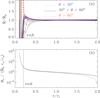Fig. 1. Radial dependence of (a) Ṁ for different latitude ranges, and (b) Mr (solid line) for Model A. The dotted line in (b) refers to the mass within the computational domain only, so it vanishes on r = rout.

whose average over θ and t, $⟨\dot{M}⟩={\int }_0^{\pi }{\int }_{t_0}^{t_0+T}\dot{M}\mathrm{d}tsin\theta \mathrm{d}\theta$, is close to the initial value Ṁ₀. This is not too surprising, but it should be emphasized that this is not enforced as a condition. The good agreement suggests that the open boundary condition at the bottom draws in a similar amount of mass at the inner boundary as what is lost at the outer boundary.

To get a sense of the radial mass distribution in our model, we plot in Fig. 1b the cumulative mass,

$$\begin{array}{c}\hfill M_r(r,\theta ,t)={\displaystyle {\int }_r^{\infty }4\pi r^{\prime 2}\overline{\rho }(r\prime ,\theta ,t)\mathrm{d}r\prime ,}\end{array}$$(28)

for different values of θ at t = 858. We see that the total mass at r = r_in is about 7000 mass units; one mass unit here is Ṁ₀r_c/c_s. The mass above the surface is about 10, so 99.9% of the total mass in the computational domain is contained in the stellar envelope in r_in ≤ r ≤ R. Thus, if no mass was replenished on the inner boundary, the time it would take to lose all mass at the initial rate would be τ_massloss = M/Ṁ = 7000.

We emphasize at this point that the full stellar mass is undetermined, because the value of Newton’s constant G never enters on its own. We could, in principle, constrain it by assuming, for example, that the density in the core is constant and equal to that at r = r_in. This would give for the minimal core mass M_core ≫ 36 000, which is five times the mass in the envelope. Using GM_core = 2, we find $G\ll 6\times {10}^{-5}{c_{\text{s}}}^3/{\dot{M}}_0$, which is satisfied by a large margin for the values quoted above. We stress, however, that this estimate was done only for illustrative purposes.

3.2. Oscillatory model at solar rotation rate

We focus on a simulation with the solar value of the angular velocity, that is, $\stackrel{\sim }{\mathrm{\Omega }}=0.2$ (Model A). In this case, the magnetic field is oscillatory, but in a rather nonlinear fashion; see Fig. 2, where we plot the time dependence of the three magnetic field components at one point in the wind. The ${\overline{B}}_r$ component is positive most of the time and much smoother than the ${\overline{B}}_{\theta }$ and ${\overline{B}}_{\varphi }$ components. The period T is about 41 time units. This corresponds to about 0.1 yr, which is short compared with the actual solar 22 year cycle, but still about five times longer than the cycle period in the model of Perri et al. (2020). Their parameters are otherwise comparable to ours: η_T ≈ 4 × 10¹⁴ cm² s⁻¹ in both models, Ṁ = 3 × 10⁻¹⁴ M_⊙ yr⁻¹ (a third of our value), an Alfvén radius of about two stellar radii, and a domain size of 20 solar radii (twice our value).

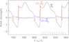Fig. 2. Time series of the three magnetic field components at one point for Model A. Here, ${\overline{B}}_{\theta }$ and ${\overline{B}}_{\varphi }$ are multiplied by 25 to make those components better visible. We note that all three components of $\overline{\mathit{B}}$ are asymmetric about zero. The 12 long tick marks on the lower abscissa show the times for which snapshots will be discussed later on.

3.3. Magnetic field geometry

In Fig. 3 we show a sequence of magnetic field visualizations at different times. To make the magnetic field in the outer parts better visible, we multiply B_ϕ by r². Here, we show the time span from $\stackrel{\sim }{t}=814$ to 858, covering just a little over a period. We overplot the surfaces where ${\overline{U}}_r$ is transalfvénic (solid white lines), that is, where ${\overline{U}}_r$ exceeds the Alfvén speed $v_{\text{A}}={({\overline{\mathit{B}}}^2/{\mu }_0\overline{\rho })}^{1/2}$. The surface is corrugated, but its mean radius is around 0.4 r_c. We also shows the surfaces where ${\overline{U}}_r$ is transmagnetosonic, that is, where ${\overline{U}}_r$ exceeds the fast magnetosonic speed c_ms (dashed white line), which obeys $c_{\text{ms}}^2=c_{\text{s}}{}^2+v_{\text{A}}{}^2$. The mean radius of the magnetosonic surface is close to r_c.

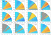Fig. 3. Color representation of r2Bϕ(r, θ) for different times for Model A. The nearly concentric red solid lines show the surfaces where ${\overline{U}}_r$ is transalfvénic and the red dashed ones show the surfaces where it is transmagnetosonic. The times correspond to the long tick marks of Fig. 2.

Butterfly diagrams of ${\overline{B}}_r(\theta ,t)$ and ${\overline{B}}_{\varphi }(\theta ,t)$ are shown in Fig. 4. The field in the wind does not show any migration in latitude, as is expected from models of the solar dynamo. Figure 5 shows only the inner part of the domain. We see regions with open and closed field lines at different times. However, there is no clear magnetic field migration that manifests itself in the Sun in a Maunder’s butterfly diagram of sunspot locations versus time and latitude.

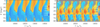Fig. 4. Butterfly diagrams of Br(r, θ) and Bϕ(r, θ) for Model A at r/rc = 1.9. Again the asymmetry of those components with respect to zero, which is different from the properties of the solar magnetic field.

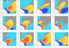Fig. 5. Similar to Fig. 3, but this time with a color representation of Bϕ(r, θ) showing only the region close to the center. Note the occurrence of V-shaped field lines during certain times at 822 ≤ t ≤ 834, and 846. The field shows radial outward migration during certain times: negative Bϕ at low latitudes for 814 ≤ t ≤ 826, and positive Bϕ at midlatitudes for 834 ≤ t ≤ 854.

It is interesting to note the appearance of V-shaped field lines in the panels for t = 822−834 and perhaps also for t = 846. This means that there are magnetic field lines in the wind that are not anchored in the star. This may be a bit surprising, but we have to remember that the magnetic field is time-dependent and the medium electrically conducting. The time-varying magnetic field can therefore induce toroidal currents in the stellar wind, which then produce poloidal field lines that are closed outside the star. This phenomenon may be similar to what is known as “switchbacks” in the solar wind (Bale et al. 2019; Squire et al. 2020).

3.4. Poynting flux

The wind carries with it not only mass, but also kinetic and magnetic energies. The latter is quantified by the mean Poynting flux,

$$\begin{array}{c}\hfill F_{\mathrm{Poy}}(r,t)={\displaystyle \oint }(\overline{\mathit{E}}\times \overline{\mathit{B}}/{\mu }_0)·\mathrm{d}\mathit{S},\end{array}$$(29)

where $\overline{\mathit{E}}={\eta }_{\text{T}}{\mu }_0\overline{\mathit{J}}-\alpha \overline{\mathit{B}}-\overline{\mathit{U}}\times \overline{\mathit{B}}$ is the mean electric field. The magnetic energy loss is then Ė_M = 4πr²F_Poy. In the steady state, ⟨Ė_M⟩ would be independent of r if there was no Ohmic dissipation and no conversion between kinetic and magnetic energies in the wind.

As a good estimate for the magnetic energy loss of the solar wind, Brandenburg et al. (2011) computed ${\dot{E}}_{\mathrm{M}}(r)\approx 4\pi r^2⟨({\overline{\mathit{B}}}^2/2{\mu }_0){\overline{U}}_r⟩$, which they found to be on the order of 10¹⁸ W and slowly decreasing with radius. Estimating the total magnetic energy content within the convection zone based on a mean field of 300 G over the convection zone of volume $4\pi (R^3-r_{\text{in}}^3)/3$, we find a time scale of about 10 years, which is comparable with the solar cycle period.

Figure 6 shows the latitudinal dependence of Ė_M at different times for Model A. It depends not only on latitude and time, but also somewhat on radius. There is a window at high latitudes where it is almost constant in θ, but the width of this window changes with time. It can have a width of over 45° (e.g., at t = 818 and 858), but it can also be almost nonexistent (e.g., at t = 842). Comparing with Fig. 3, we see that this window of nearly constant Ė_M corresponds to regions where the radial field in the wind ist mostly negative. The dips in Ė_M correspond to regions where the radial field is weak and changes sign. Near the equator, Ė_M shows a sharp drop for most times, except for t = 826. Again, comparing with Fig. 3, we see that nothing special happens near those dips, except that for t = 826 the field is a bit weaker. These dips are probably a consequence of the radial field reversal in the equatorial plane and the existence of a field component that is purely vertical to the equatorial plane, thus inhibiting the wind.

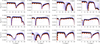Fig. 6. Latitudinal dependence of the magnetic energy loss at different times for Model A. Note the occurrence of a plateau for small values of θ for 814 ≤ t ≤ 830 and after t = 854.

Next, we look at the radial dependence of the kinetic and magnetic energy losses for different times and latitudes. The result is shown in Fig. 7, where we define compute them as

$$\begin{array}{cc}& {\dot{E}}_{\mathrm{K}}=4\pi r^2(\overline{\rho }{\overline{\mathit{U}}}^2/2)u_r,\hfill \end{array}$$(30)

$$\begin{array}{cc}& {\dot{E}}_{\mathrm{M}}=4\pi r^2({\overline{\mathit{B}}}^2/2{\mu }_0)u_r,\hfill \end{array}$$(31)

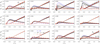Fig. 7. Radial dependence of ĖK and ĖM for different latitude ranges at different times for Model A. Note that ĖM has been multiplied by a factor of 20. ĖK shows only little variability and always increases radially outward, while ĖM has a maximum near the Alfvén surface at r/rc ≈ 0.4. The maxima are particularly high for 822 ≤ t ≤ 826.

respectively. It turns out that Ė_M is much smaller than Ė_M. To accommodate both quantities in the same plot, we have multiplied Ė_M by a factor of 20.

We see that Ė_K increases with radius. This is a peculiar feature of isothermal models which is absent both in isentropic models with constant specific entropy and in nonisentropic models with variable specific entropy; see Figs. 9.18 and 9.20 of Brandenburg (2003), respectively. This is mainly because in those models the sound speed decreases with radius in such a way that the Mach number still increases, just as in the isothermal models. Thus, the basic dynamics is similar in that the flow becomes supersonic. In isothermal models, where the sound speed is constant, this transition must always be accompanied by a radial increase of the wind speed. In this sense, a polytropic model would seem more realistic, but it would still ignore the internal energy or entropy equation, which would be even more important for making our models more realistic, as is discussed below; see Sect. 3.8.

We also see that for t = 826, when the field was a bit weaker further out in the wind (Fig. 3), the kinetic energy loss is particularly strong around the Alfvén surface; see Fig. 7. At other times, especially for t ≤ 842 ≤ 850, the kinetic energy loss is generally much weaker. Comparing again with Fig. 3, this corresponds to times when the radial field near the equator is strong.

In Fig. 8, we show Ė_M and Ė_K for r ≤ r_c as a semilogarithmic representation. We see that Ė_M ≈ Ė_K at r/r_c ≈ 0.4. The radial profiles of Ė_K are fairly independent of θ and t. This is because the wind is rather powerful and not much affected by rotation or magnetic fields, which are the main factors that provide non-spherically symmetric contributions to the system.

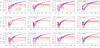Fig. 8. Similar to Fig. 7, for a semilogarithmic representation, without having rescaled ĖM. Blue (red) lines indicate kinetic (magnetic) energy losses. Note that ĖM ≈ ĖK near the Alfvén surface at r/rc ≈ 0.4, which is marked by a vertical line.

It is interesting to note that Ė_M(r) has a maximum at r ≈ r_c/2. This radius is a certain distance above the stellar surface and still below the critical point. This radius coincides with the Alfvén radius; see Fig. 3. This is the point where most of the star’s magnetic energy has been deposited into the wind. In the Sun, we expect that this energy depositions occurs in the corona. One may tentatively associate the location of the maximum of Ė_M(r) with some representation of the star’s corona, although it is unclear whether there is any relation to the real corona of the Sun.

At large radii, r ≫ r_c, the magnetic energy loss declines slowly with radius. Such a decline has also been seen for the solar wind (Brandenburg et al. 2011). In the Sun, it may be connected with the conversion of magnetic energy into heat.

3.5. Angular momentum flux

There are no sinks or sources to the angular momentum density, $\overline{\rho }{\varpi }^2\mathrm{\Omega }$, and it therefore satisfies a conservation equation of the form (Mestel 1968, 1999)

$$\begin{array}{c}\hfill \frac{\partial }{\partial t}\left(\overline{\rho }{\varpi }^2\mathrm{\Omega }\right)=-\mathbf{\nabla }·{\mathit{F}}^{\mathrm{AM}},\end{array}$$(32)

where

$$\begin{array}{c}\hfill {\mathit{F}}^{\mathrm{AM}}=\overline{\rho }{\varpi }^2\mathrm{\Omega }\overline{\mathit{U}}-\varpi {\overline{B}}_{\varphi }\overline{\mathit{B}}/{\mu }_0-\overline{\rho }{\nu }_{\mathrm{T}}{\varpi }^2\mathbf{\nabla }\mathrm{\Omega }\end{array}$$(33)

is the angular momentum flux. Analogously to the energy loss, the expression for the angular momentum loss is $\dot{J}=4\pi r^2{F}_r^{\mathrm{AM}}$, which is shown in Fig. 9 for 1.5 ≤ r/r_c ≤ 2 for the kinetic, magnetic, and viscous contributions, ${\dot{J}}_{\mathrm{K}}$, ${\dot{J}}_{\mathrm{M}}$, and ${\dot{J}}_{\nu }$, respectively. We see that the angular momentum flux is highly structured, with positive and negative contributions at different latitudes and times. At these radii, the kinetic term proportional to ${\overline{U}}_{\varphi }{\overline{U}}_r$ dominates over the magnetic term proportional to ${\overline{B}}_{\varphi }{\overline{B}}_r$, and the turbulent viscous term is negligible.

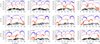Fig. 9. Latitudinal dependence of the angular momentum loss $\dot{J}(r,\theta ,t)$ for 1.5 ≤ r/rc ≤ 2 at different times for Model A. The blue (red) lines refer to kinetic (magnetic) contributions, and the black lines denote the turbulent viscous contribution. Positive (negative) values are shown as solid (dotted) lines. Note the strong latitudinal variability of $\dot{J}$.

The strongly negative contributions to the angular momentum flux are unexpected and may be connected with the time dependence of the solution. It may be of interest to study angular momentum fluxes along magnetic field lines; see the work of Pantolmos & Matt (2017), who compare flow speeds along different field lines. For our unsteady wind solutions, this procedure may no longer be particularly advantageous. However, to get some idea about the latitudes contributing to the negative angular momentum flux, we show in Fig. 10 the radial dependence of the time- and latitude-averaged profiles of $\dot{J}$ separately for the cones θ < 70° (away from the equator) and θ ≥ 70° (around the equator). We see that negative angular momentum fluxes dominate and originate mainly from regions away from the equator. Nevertheless, in the range 0.2 ≤ r/r_c ≤ 0.6, ${\dot{J}}_{\mathrm{K}}$ and ${\dot{J}}_{\mathrm{M}}$ can be of comparable magnitude, as is expected from the theory of Weber & Davis (1967). This range agrees well with the Alfvén radius; see Fig. 3.

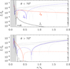Fig. 10. Time averaged radial profiles of latitudinally averaged $\dot{J}$ for θ < 70° (upper panel) and θ > 70° (lower panel). The blue (red) lines refer to kinetic (magnetic) contributions, and the black lines denote the turbulent viscous contribution. Positive (negative) values are shown as solid (dotted) lines. The kinetic contributions from different times are shown as gray lines. The gray background on the left indicates the location of the stellar envelope.

To understand the variability of Ω and the occurrence of negative values at certain times, we show in Fig. 11 angular velocity contours superimposed on a color representation of ${\overline{U}}_r(r,\theta )$. Interestingly, Ω is often negative over an extended range of mid-latitudes. As we have seen above, this is chiefly responsible for the inward angular momentum transport discussed above. This could be related to our rather primitive modeling of the hydrodynamics inside the star, which lacks realistic differential rotation, for example. We return to this question briefly in the conclusions. We also note that ${\overline{U}}_r(r,\theta )$ shows clear latitudinal variations. The occurrence of regions with negative angular momentum transport is interesting in view of the recent discovery of fast wind episodes observed with Parker Solar Probe at certain longitudes (Finley et al. 2020, 2021). Our model is of course axisymmetric and cannot address longitudinal variations, but it reminds us that negative angular momentum transport is not impossible.

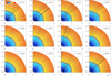Fig. 11. Angular velocity contours superimposed on a color representation of ${\overline{U}}_r(r,\theta )$ for Model A. Positive (negative) values of Ω are shown as solid (dotted) black contours. Note the extended region at midlatitudes were Ω < 0.

We should point out that $\dot{J}$ is given here in standard units where Ṁ = c_s = 1. Therefore, Fig. 9 can be directly interpreted as a plot of the mean-field (MF) analogue of the Shakura & Sunyaev (1973) parameter,

$$\begin{array}{c}\hfill {\alpha }_{\mathrm{SS}}^{\mathrm{MF}}=(\overline{\rho }{\overline{U}}_r{\overline{U}}_{\varphi }-{\overline{B}}_r{\overline{B}}_{\varphi }/{\mu }_0)/c_{\mathrm{s}}^2.\end{array}$$(34)

Here, the superscript MF indicates that this expression is applied to the two-dimensional mean fields rather than to the fluctuations, as in the usual turbulent case. This parameter is also frequently used in solar wind studies (see Eq. (2) of Finley et al. 2019); see also Keppens & Goedbloed (1999), Réville et al. (2015), and Pantolmos & Matt (2017) for earlier two-dimensional stellar wind models.

The angular momentum in the dynamo zone is J_* ≈ 68 in our units. Owing to cancelation, it is difficult to determine reliable values of $\dot{J}$ and ${\alpha }_{\mathrm{SS}}^{\mathrm{MF}}$, but for the purpose of a preliminary assessment, it suffices to estimate $\dot{J}\approx 0.01$. As we discuss below in more detail, there can be certain periods where $\dot{J}$ can even be negative. This then implies spindown or spinup at a rate τ_spin ≈ 7000, which is indeed similar to the value of τ_massloss quoted in Sect. 2.5. It may well be that ${\alpha }_{\mathrm{SS}}^{\mathrm{MF}}$ is much less than 0.01. This would then imply an even larger value of τ_spindown.

3.6. Resulting dynamo parameters

In our model, differential rotation is automatically established as a result of magnetic braking. Since our turbulent viscosity is assumed to be purely isotropic, differential rotation can only result from the torque on the star established by the magnetized wind (Mestel 1968). This leads to a nearly constant angular momentum per unit mass, that is, ϖ²Ω ≈ const. The contours of constant angular velocity tend to approach a pattern that is close to cylindrical, as will be discussed below in the context of rapid rotation. Given that Ω ∝ ϖ⁻², the angular velocity difference between the r_in and R is $\mathrm{\Delta }\mathrm{\Omega }=(1-r_{\text{in}}^2/R^2){\mathrm{\Omega }}_0=0.75{\mathrm{\Omega }}_0$. Therefore, we have for the second dynamo parameter in Eq. (20) the values C_Ω = 75, 375, and 3750 for $\stackrel{\sim }{\mathrm{\Omega }}=0.2$, 1, and 10, respectively. The first dynamo parameter in Eq. (20) is C_α = 125, where we have used ${\stackrel{\sim }{\alpha }}_0\equiv {\alpha }_0/c_{\text{s}}=0.05$ for Model A, and η_T = 8 × 10⁻⁵r_cc_s.

3.7. Rapid rotation

The study of models at rapid rotation is motivated by the interest in understanding the evolution of magnetic activity of young stars, that is, before they have slowed down to the solar rotation rate. For us, there is also another motivation in that all our models were of α² type, that is, the Ω effect was weak and C_Ω was not much larger than C_α, as required for an αΩ dynamo (Brandenburg & Subramanian 2005). To increase C_Ω, the rotation rate could be increased. Another possibility is to lower C_α. However, to prevent the dynamo from decaying, one would need to decrease η_T even further, but this is computationally difficult.

For rapid rotation, the magnetic field lines and contours of the toroidal magnetic field are much more concentrated to the bottom of the dynamo region, r ≈ r_in. At faster rotation, the contours become more cylindrical. This is an effect of the Taylor–Proudman theorem and results generally in small variations along the rotation axis.

The Taylor–Proudman theorem applies primarily to the angular velocity contours. This can be seen by writing the relevant part of the $\overline{\mathit{U}}·\mathbf{\nabla }\overline{\mathit{U}}$ nonlinearity of Eq. (2) in the form

$$\begin{array}{c}\hfill \widehat{\mathit{\varphi }}·\mathbf{\nabla }\times {(-\overline{\mathit{U}}·\mathbf{\nabla }\overline{\mathit{U}})}_{\mathrm{p}}=\varpi \frac{\partial }{\partial z}{\mathrm{\Omega }}^2+\dots ,\end{array}$$(35)

where $\mathrm{\Omega }={\overline{U}}_{\varphi }/\varpi$ is the local angular velocity, and the dots indicate the presence of other terms not relevant here. In Fig. 12a we show contours of Ω together with a color-coded representation of ${\overline{U}}_r$. We see that the Ω contours are already strongly cylindrical for $\stackrel{\sim }{\mathrm{\Omega }}=1$. As we increase the value of $\stackrel{\sim }{\mathrm{\Omega }}$ to 10, the cylindrical contours begin to extent much further out along the rotation axis; see Fig. 12b.

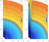Fig. 12. Angular velocity contours superimposed on a color representation of ${\overline{U}}_r(r,\theta )$ for Model B (a) with $\stackrel{\sim }{\mathrm{\Omega }}=1$ and Model C (b) with $\stackrel{\sim }{\mathrm{\Omega }}=10$. The nearly concentric red solid lines show the surfaces where ${\overline{U}}_r$ is transalfvénic and the red dashed ones show the surfaces where it is transmagnetosonic.

For $\stackrel{\sim }{\mathrm{\Omega }}=10$, the radial velocity develops a marked indentation inside of what is known as the inner tangent cylinder where

$$\begin{array}{c}\hfill \varpi \ge r_{\mathrm{in}}(\mathrm{inner}\mathrm{tangent}\mathrm{cylinder});\end{array}$$(36)

see Fig. 12b. Here the outflow is suppressed and supersonic flows occur only for z ≥ 2r_c ≈ r_out, that is, near the outer boundary of the computational domain. For $\stackrel{\sim }{\mathrm{\Omega }}=1$, by comparison, the contours of ${\overline{U}}_r(r,\theta )$ are almost perfectly spherically symmetric – much more so than even for the case with $\stackrel{\sim }{\mathrm{\Omega }}=0.2$; cf. Fig. 11. Similar results have also been found by Washimi & Shibata (1993) in their rotating models where a central dipole magnetic field was assumed.

It turns out that our models are now no longer oscillatory and are thus still not of αΩ type, contrary to what was originally hoped for. Visualizations of the toroidal and poloidal fields for Models B and C are shown in Figs. 13 and 14, respectively. The fields are strong only inside the star, where the dynamo is active. Outside the star, the field is much weaker and not visible in our graphical representation, but it is never vanishing.

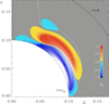Fig. 13. Magnetic field lines superimposed on a color representation of ${\overline{B}}_{\varphi }(r,\theta )$ for Model B with $\stackrel{\sim }{\mathrm{\Omega }}=1$. Strong fields only occur near r = rin; the weak-field regions elsewhere cannot be seen.

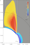Fig. 14. Similar to Fig. 13, but for Model C with $\stackrel{\sim }{\mathrm{\Omega }}=10$. Stronger fields now extend along the axis outside the star.

To discuss the nonoscillatory nature of these two models, it is useful to consider the dynamo parameters C_α and C_Ω. We find C_α = 125 and C_Ω = 3750 for η_T = ν_T = 8 × 10⁻⁵; see Table 1. To get an idea about the latitudinal variation of the magnetic field in the wind, the plot Ė_M as a function of θ for different radii. The result is shown in Fig. 15. It turns out that the magnetic activity is confined to a narrow cone with an opening angle of about 15°.

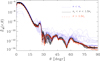Fig. 15. Latitudinal dependence of ĖM for different radius ranges for Model B. Note that ĖM is large only near the axis.

Noticeable magnetic energy losses are found only near the rotation axis. As a function of radius, similarly to the case of slow rotation, Ė_M(r) has a maximum somewhere in R < r < r_c, which is where the Alfvén point lies. Furthermore, Model B has a much smaller magnetic energy loss at large radii than Model A.

The model shows similarities with earlier simulations of outflows emanating from stellar accretion disk dynamos (von Rekowski et al. 2003; von Rekowski & Brandenburg 2004), but there the opening angle was closer to 30°. In the present simulations, the opening angle is essentially zero. It corresponds to a cylinder in which most of the magnetic fields are ejected, although the flow speed here is strongly reduced.

For these rapidly rotating models, we expect significant outward angular momentum transport. To demonstrate this in more detail, we show in Fig. 16 the radial profiles of the latitudinally averaged $\dot{J}$ for Models A–C for the kinetic, magnetic, and viscous contributions, just as we did in Fig. 10. Since Models B and C are steady, time averaging is only needed for Model A.

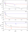Fig. 16. Radial profiles of the latitudinally averaged $\dot{J}$ for Models A–C in panels a–c. The blue (red) lines refer to kinetic (magnetic) contributions, and the black lines denote the turbulent viscous contribution. Positive (negative) values are shown as solid (dotted) lines. The total (kinetic, magnetic, and viscous) angular momentum transport is dominated by the kinetic contribution, except for Model A, where the magnetic contribution is rather strong, but negative in the outer parts.

Figure 16 shows that in Models B and C, the angular momentum transport is outward and $\dot{J}$ is independent of r throughout most of the wind. For Model A, however, the time-averaged angular momentum transport becomes negative some distance away from the Alfvén point. Furthermore, $\dot{J}$ is more than ten times larger in Model C than in the ten times more slowly rotating Model B. For Model B, the viscous contribution exceeds the magnetic one at all radii, while in Model C, the magnetic contribution exceeds the viscous one for r/r_c > 1.5. Inside the star, the angular momentum transport is negative and caused by a strong poleward circulation. The viscous contribution is also rather strong, but positive.

3.8. Comparison of the plasma betas for our models

We have seen that in Model A with the slowest rotation, the angular momentum flux was occasionally inward, especially at midlatitudes. We then considered Models B and C with faster rotation in the hope that not only the outward angular momentum flux would be outward, but also that the dynamo in the star would be in the αΩ regime. We found that the angular momentum flux was then indeed outward, but the dynamo was still in the α² regime. In the introduction, we did already emphasize that the lack of a cool photosphere just beneath the corona was ignored. This makes it generally very difficult to reach low plasma betas, which we define as

$$\begin{array}{c}\hfill \beta =2\rho c_{\mathrm{s}}^2/{\mathit{B}}^2.\end{array}$$(37)

In Fig. 17, we plot the radial dependencies of the minimum value of β, β_min, for Models A–C. We see that the largest values of β_min occur for Model B with an intermediate angular velocity. Increasing the angular velocity further (Model C) increases the field strength and does therefore also lead to a smaller value of β_min. The smallest values occur for Model A. This is mainly because Model A is the only model where the magnetic field in the wind is of comparable strength at all latitudes. For faster rotation, the field in the wind is strongly concentrated around the axis.

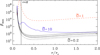Fig. 17. Radial dependence of the plasma β for Models A (dotted black lines), B (dashed red line), and C (solid blue line).

Let us now return to the potential role of the photosphere. The photosphere of a star is the region where it cools and loses specific entropy. Everywhere else in the wind, the specific entropy does not change much, and therefore the potential enthalpy must be approximately constant (von Rekowski et al. 2003). The potential enthalpy is defined as H = h + Φ, where h = c_pT is the specific enthalpy with c_p being the specific heat at constant pressure and T the temperature, and Φ = −GM/r is the potential energy. Hydrostatic equilibrium requires that

$$\begin{array}{c}\hfill 0=-\mathbf{\nabla }H+h\mathbf{\nabla }s/c_{\mathrm{p}},\end{array}$$(38)

where s is the specific entropy. For the corona, this implies T = GM/rc_p ≈ 2 × 10⁶ K, which is realistic and agrees also with our model. Toward the photosphere, T decreases abruptly because of surface cooling, and therefore the density increases abruptly. Thus, the density would then be much larger than what was possible in our models. This, in turn, would allow us to reach much larger field strengths and therefore smaller plasma betas.

Another important consequence of having larger densities in the stellar envelope would be that the angular velocity at the stellar surface would always be in the prograde direction. In our present models, this is not always the case, as can be seen from Fig. 18, where we show the radial and azimuthal velocities at the stellar surface. We see that the local rotational velocity is there occasionally in the retrograde direction, especially near the equator.

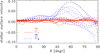Fig. 18. ${\overline{U}}_r$ (red solid lines) and ${\overline{U}}_{\varphi }$ (blue dashed lines) at the stellar surface at r = R as a function of colatitude for the same times as in Fig. 10. ${\overline{U}}_r$ is usually positive, but $|{\overline{U}}_{\varphi }|$ is much larger and most of the time in the prograde direction, but sometimes it is retrograde, which is a consequence of the low moment of inertia of the stellar envelope in our model.

4. Conclusions

Our work has shown that a simplified realization of a dynamo with a stellar wind can easily be treated self-consistently in one and the same model, provided certain compromises are being made. The assumption of an isothermal equation of state has simplified matters conceptionally. Relaxing this restriction would allow us to include the energy deposition in the corona and to model the effects of a sharp density drop at the stellar surface. This might require a significant increase in resolution near the surface, which in turn requires the use of a nonuniform mesh. Another restriction has been the use of a relatively large turbulent magnetic diffusivity and viscosity. This was mainly needed to resolve shocks that develop within the wind. Those typically emerged in response to rapid changes in the magnetic field. This could probably be avoided by allowing for an additional shock viscosity, but this has been avoided in the present work. On the other hand, the angular momentum flux associated with turbulent viscosity was already negligible, so its presence may not have caused any artifacts.

Future work might involve the inclusion of a Λ effect (Rüdiger 1980, 1989), which would allow for the development of differential rotation in the stellar envelope. Without including the effects of stellar winds, such models with combined α and Λ effects were studied by Brandenburg et al. (1990, 1991), who found significant alignment of the Ω contours with the rotation axis unless the baroclinic term was also included (Brandenburg et al. 1992). But this may change when their boundary condition on r = R is replaced by a continuous transition to the solar exterior; see Warnecke et al. (2013) for spherical convection simulations with a simplified representation of a stellar corona.

The inclusion of the Λ effect might allow us to model the stellar dynamo more realistically. It would be interesting to see how this affects the angular momentum transport and whether it could help in producing predominantly outward angular momentum transport in cases of slow rotation. It might then allow us to study dynamos in the αΩ regime. This has not been possible in the present model for reasons that are not entirely clear, because the value of C_Ω was thought to be already large enough. There could have been other side effects arising from the coupling to the outflow that are not yet fully understood. Nevertheless, it is interesting to note that the inward angular momentum transport occurs even in the Sun within fast-wind regions at certain longitudes; see Finley et al. (2020, 2021).

Another important aspect requiring further attention is the study of angular momentum losses from mean-field stresses. Our work has shown that the angular momentum loss can be quantified in terms of a nondimensional Shakura–Sunyaev parameter. This is a somewhat unusual concept in the context of stellar winds, but it may help putting the theories of turbulent stellar winds and accretion disks on a common footing.

Acknowledgments

We thank the referee for many useful remarks and suggestions that have significantly improved the manuscript. This work was supported in part through the Erasmus+ Programme of the European Union (P.J.) and the Swedish Research Council, grant 2019-04234 (A.B.). We acknowledge the allocation of computing resources provided by the Swedish National Allocations Committee at the Center for Parallel Computers at the Royal Institute of Technology in Stockholm.

References

All Tables

All Figures

	Fig. 1. Radial dependence of (a) Ṁ for different latitude ranges, and (b) Mr (solid line) for Model A. The dotted line in (b) refers to the mass within the computational domain only, so it vanishes on r = rout.
In the text

Fig. 2. Time series of the three magnetic field components at one point for Model A. Here, ${\overline{B}}_{\theta }$ and ${\overline{B}}_{\varphi }$ are multiplied by 25 to make those components better visible. We note that all three components of $\overline{\mathit{B}}$ are asymmetric about zero. The 12 long tick marks on the lower abscissa show the times for which snapshots will be discussed later on.

In the text

	Fig. 3. Color representation of r2Bϕ(r, θ) for different times for Model A. The nearly concentric red solid lines show the surfaces where ${\overline{U}}_r$ is transalfvénic and the red dashed ones show the surfaces where it is transmagnetosonic. The times correspond to the long tick marks of Fig. 2.
In the text

	Fig. 4. Butterfly diagrams of Br(r, θ) and Bϕ(r, θ) for Model A at r/rc = 1.9. Again the asymmetry of those components with respect to zero, which is different from the properties of the solar magnetic field.
In the text

	Fig. 5. Similar to Fig. 3, but this time with a color representation of Bϕ(r, θ) showing only the region close to the center. Note the occurrence of V-shaped field lines during certain times at 822 ≤ t ≤ 834, and 846. The field shows radial outward migration during certain times: negative Bϕ at low latitudes for 814 ≤ t ≤ 826, and positive Bϕ at midlatitudes for 834 ≤ t ≤ 854.
In the text

	Fig. 6. Latitudinal dependence of the magnetic energy loss at different times for Model A. Note the occurrence of a plateau for small values of θ for 814 ≤ t ≤ 830 and after t = 854.
In the text

	Fig. 7. Radial dependence of ĖK and ĖM for different latitude ranges at different times for Model A. Note that ĖM has been multiplied by a factor of 20. ĖK shows only little variability and always increases radially outward, while ĖM has a maximum near the Alfvén surface at r/rc ≈ 0.4. The maxima are particularly high for 822 ≤ t ≤ 826.
In the text

	Fig. 8. Similar to Fig. 7, for a semilogarithmic representation, without having rescaled ĖM. Blue (red) lines indicate kinetic (magnetic) energy losses. Note that ĖM ≈ ĖK near the Alfvén surface at r/rc ≈ 0.4, which is marked by a vertical line.
In the text

	Fig. 9. Latitudinal dependence of the angular momentum loss $\dot{J}(r,\theta ,t)$ for 1.5 ≤ r/rc ≤ 2 at different times for Model A. The blue (red) lines refer to kinetic (magnetic) contributions, and the black lines denote the turbulent viscous contribution. Positive (negative) values are shown as solid (dotted) lines. Note the strong latitudinal variability of $\dot{J}$.
In the text

Fig. 10. Time averaged radial profiles of latitudinally averaged $\dot{J}$ for θ < 70° (upper panel) and θ > 70° (lower panel). The blue (red) lines refer to kinetic (magnetic) contributions, and the black lines denote the turbulent viscous contribution. Positive (negative) values are shown as solid (dotted) lines. The kinetic contributions from different times are shown as gray lines. The gray background on the left indicates the location of the stellar envelope.

In the text

	Fig. 11. Angular velocity contours superimposed on a color representation of ${\overline{U}}_r(r,\theta )$ for Model A. Positive (negative) values of Ω are shown as solid (dotted) black contours. Note the extended region at midlatitudes were Ω < 0.
In the text

	Fig. 12. Angular velocity contours superimposed on a color representation of ${\overline{U}}_r(r,\theta )$ for Model B (a) with $\stackrel{\sim }{\mathrm{\Omega }}=1$ and Model C (b) with $\stackrel{\sim }{\mathrm{\Omega }}=10$. The nearly concentric red solid lines show the surfaces where ${\overline{U}}_r$ is transalfvénic and the red dashed ones show the surfaces where it is transmagnetosonic.
In the text

	Fig. 13. Magnetic field lines superimposed on a color representation of ${\overline{B}}_{\varphi }(r,\theta )$ for Model B with $\stackrel{\sim }{\mathrm{\Omega }}=1$. Strong fields only occur near r = rin; the weak-field regions elsewhere cannot be seen.
In the text

	Fig. 14. Similar to Fig. 13, but for Model C with $\stackrel{\sim }{\mathrm{\Omega }}=10$. Stronger fields now extend along the axis outside the star.
In the text

	Fig. 15. Latitudinal dependence of ĖM for different radius ranges for Model B. Note that ĖM is large only near the axis.
In the text

Fig. 16. Radial profiles of the latitudinally averaged $\dot{J}$ for Models A–C in panels a–c. The blue (red) lines refer to kinetic (magnetic) contributions, and the black lines denote the turbulent viscous contribution. Positive (negative) values are shown as solid (dotted) lines. The total (kinetic, magnetic, and viscous) angular momentum transport is dominated by the kinetic contribution, except for Model A, where the magnetic contribution is rather strong, but negative in the outer parts.

In the text

	Fig. 17. Radial dependence of the plasma β for Models A (dotted black lines), B (dashed red line), and C (solid blue line).
In the text

Fig. 18. ${\overline{U}}_r$ (red solid lines) and ${\overline{U}}_{\varphi }$ (blue dashed lines) at the stellar surface at r = R as a function of colatitude for the same times as in Fig. 10. ${\overline{U}}_r$ is usually positive, but $|{\overline{U}}_{\varphi }|$ is much larger and most of the time in the prograde direction, but sometimes it is retrograde, which is a consequence of the low moment of inertia of the stellar envelope in our model.

In the text

References

- Bale, S. D., Badman, S. T., Bonnell, J. W., et al. 2019, Nature, 576, 237 [Google Scholar]
- Biermann, L. 1951, Z. Astrophys., 29, 274 [NASA ADS] [Google Scholar]
- Brandenburg, A. 2003, in Advances in Nonlinear Dynamos, The Fluid Mechanics of Astrophysics and Geophysics, eds. A. Ferriz-Mas, & M. Núñez (London and New York: Taylor & Francis), 9 [Google Scholar]
- Brandenburg, A., & Subramanian, K. 2005, Phys. Rep., 417, 1 [Google Scholar]
- Brandenburg, A., Moss, D., Rüdiger, G., & Tuominen, I. 1990, Sol. Phys., 128, 243251 [Google Scholar]
- Brandenburg, A., Moss, D., Rüdiger, G., & Tuominen, I. 1991, Geophys. Astrophys. Fluid Dyn., 61, 179 [Google Scholar]
- Brandenburg, A., Moss, D., & Tuominen, I. 1992, A&A, 265, 328 [NASA ADS] [Google Scholar]
- Brandenburg, A., Subramanian, K., Balogh, A., & Goldstein, M. L. 2011, ApJ, 734, 9 [Google Scholar]
- Chamberlain, J. W. 1960, ApJ, 131, 47 [Google Scholar]
- Cole, E., Brandenburg, A., Käpylä, P. J., & Käpylä, M. J. 2016, A&A, 593, A134 [NASA ADS] [CrossRef] [EDP Sciences] [Google Scholar]
- Del Sordo, F., Guerrero, G., & Brandenburg, A. 2013, MNRAS, 429, 1686 [Google Scholar]
- Finley, A. J., Hewitt, A. L., Matt, S. P., et al. 2019, ApJ, 885, L30 [Google Scholar]
- Finley, A. J., Matt, S. P., Réville, V., et al. 2020, ApJ, 902, L4 [Google Scholar]
- Finley, A. J., McManus, M. D., Matt, S. P., et al. 2021, A&A, in press, https://doi.org/10.1051/0004-6361/202039288 [Google Scholar]
- Frank, J., King, A. R., & Raine, D. J. 1992, Accretion Power in Astrophysics (Cambridge: Cambridge Univ. Press) [Google Scholar]
- Gastine, T., Yadav, R. K., Morin, J., Reiners, A., & Wicht, J. 2014, MNRAS, 438, L76 [Google Scholar]
- Jabbari, S., Brandenburg, A., Kleeorin, N., Mitra, D., & Rogachevskii, I. 2015, ApJ, 805, 166 [Google Scholar]
- Jakab, J., & Brandenburg, A. 2020, https://doi.org/10.5281/zenodo.4284439 [Google Scholar]
- Käpylä, P. J., Käpylä, M. J., & Brandenburg, A. 2014, A&A, 570, A43 [NASA ADS] [CrossRef] [EDP Sciences] [Google Scholar]
- Keppens, R., & Goedbloed, J. P. 1999, A&A, 343, 251 [NASA ADS] [Google Scholar]
- Krause, F., & Rädler, K.-H. 1980, Mean-field Magnetohydrodynamics and Dynamo Theory (Oxford: Pergamon Press) [Google Scholar]
- Malkus, W. V. R., & Proctor, M. R. E. 1975, J. Fluid Mech., 67, 417 [Google Scholar]
- Mestel, L. 1968, MNRAS, 138, 359 [Google Scholar]
- Mestel, L. 1999, Stellar Magnetism (Oxford: Clarendon Press) [Google Scholar]
- Metcalfe, T. S., & van Saders, J. 2017, Sol. Phys., 292, 126 [Google Scholar]
- Mitra, D., Moss, D., Tavakol, R., & Brandenburg, A. 2011, A&A, 526, A138 [Google Scholar]
- Parker, E. N. 1958, ApJ, 128, 664 [Google Scholar]
- Pantolmos, G., & Matt, S. P. 2017, ApJ, 849, 83 [Google Scholar]
- Pencil Code Collaboration (Brandenburg, A., et al.) 2018, https://doi.org/10.5281/zenodo.2315093 [Google Scholar]
- Pencil Code Collaboration (Brandenburg, A., et al.) 2020, J. Open Source Softw., 5, 2684 [Google Scholar]
- Perri, B., Brun, A. S., Réville, V., & Strugarek, A. 2018, J. Plasma Phys., 84, 765840501 [Google Scholar]
- Perri, B., Brun, A. S., Réville, V., & Strugarek, A. 2020, in Magnetic Field Evolution in Solar-type Stars, IAUS 354: Solar and Stellar Magnetic Fields: Origins and Manifestations, eds. A. Kosovichev, K. Strassmeier, & M. Jardine, Proc. IAU Symp., 354, 215 [Google Scholar]
- Pinto, R. F., Brun, A. S., Jouve, L., & Grappin, R. 2011, ApJ, 737, 72 [Google Scholar]
- Réville, V., Brun, A. S., Matt, S. P., Strugarek, A., & Pinto, R. F. 2015, ApJ, 798, 116 [NASA ADS] [CrossRef] [Google Scholar]
- Roberts, P. H. 1972, Philos. Trans. R. Soc. A, 272, 663 [Google Scholar]
- Rüdiger, G. 1980, Geophys. Astrophys. Fluid Dyn., 16, 239 [NASA ADS] [CrossRef] [Google Scholar]
- Rüdiger, G. 1989, Differential Rotation and Stellar Convection: Sun and Solar-type Stars (New York: Gordon & Breach) [Google Scholar]
- See, V., Matt, S. P., Finley, A. J., et al. 2019, ApJ, 886, 120 [Google Scholar]
- Shakura, N. I., & Sunyaev, R. A. 1973, A&A, 24, 337 [NASA ADS] [Google Scholar]
- Shore, S. N. 1992, An Introduction to Astrophysical Hydrodynamics (San Diego: Academic Press) [Google Scholar]
- Squire, J., Chandran, B. D. G., & Meyrand, R. 2020, ApJ, 891, 2 [Google Scholar]
- Stix, M. 1974, A&A, 37, 121 [Google Scholar]
- van Saders, J. L., Ceillier, T., Metcalfe, T. S., et al. 2016, Nature, 529, 181 [NASA ADS] [CrossRef] [PubMed] [Google Scholar]
- von Rekowski, B., & Brandenburg, A. 2004, A&A, 420, 17 [NASA ADS] [CrossRef] [EDP Sciences] [Google Scholar]
- von Rekowski, B., Brandenburg, A., Dobler, W., & Shukurov, A. 2003, A&A, 398, 825 [NASA ADS] [CrossRef] [EDP Sciences] [Google Scholar]
- Warnecke, J., Käpylä, P. J., Mantere, M. J., & Brandenburg, A. 2013, ApJ, 778, 141 [Google Scholar]
- Washimi, H., & Shibata, S. 1993, MNRAS, 262, 936 [Google Scholar]
- Weber, E. J., & Davis, L., Jr. 1967, ApJ, 148, 217 [NASA ADS] [CrossRef] [Google Scholar]