| Issue |
A&A
Volume 646, February 2021
|
|
|---|---|---|
| Article Number | A103 | |
| Number of page(s) | 18 | |
| Section | Interstellar and circumstellar matter | |
| DOI | https://doi.org/10.1051/0004-6361/202039074 | |
| Published online | 15 February 2021 | |
Physical characterization of S169: a prototypical IR bubble associated with the massive star-forming region IRAS 12326-6245
1
Instituto de Astrofísica de La Plata (UNLP - CONICET),
La Plata, Argentina
e-mail: This email address is being protected from spambots. You need JavaScript enabled to view it.
2
Instituto de Astronomía y Física del Espacio (UBA, CONICET),
CC 67, Suc. 28,
1428
Buenos Aires, Argentina
3
Departamento de Astronomía, Universidad de Chile,
Casilla 36,
Santiago de Chile,
Chile
4
Observatório do Valongo, Universidade Federal do Rio de Janeiro,
Ladeira Pedro Antônio, 43,
Rio de Janeiro
20080-090, Brazil
5
Facultad de Ciencias Astronómicas y Geofísicas, Universidad Nacional de La Plata,
Paseo del Bosque s/n,
1900
La Plata, Argentina
6
Instituto Argentino de Radioastronomía (CCT-La Plata, CONICET; CICPBA),
C.C. No. 5,
1894
Villa Elisa, Argentina
Received:
31
July
2020
Accepted:
3
December
2020
Abstract
Aims. With the aim of studying the physical properties of Galactic IR bubbles and to explore their impact in massive star formation, we present a study of the IR bubble S169, associated with the massive star forming region IRAS 12326-6245.
Methods. We used CO (2–1),13CO (2–1), C18O (2–1), HCN (3–2), and HCO+ (3–2) line data obtained with the APEX telescope using the on-the-fly full sampling technique to study the properties of the molecular gas in the nebula and the IRAS source. To analyze the properties and distribution of the dust, we made use of images obtained from the IRAC-GLIMPSE, Herschel, and ATLASGAL archives. The properties of the ionized gas in the nebula were studied using radio continuum and Hα images obtained from the SUMSS survey and SuperCOSMOS database, respectively. In our search for stellar and protostellar objects in the region, we used point source calalogs obtained from the MSX, WISE, GLIMPSE, 2MASS, AAVSO, ASCC-2.5V3, and GAIA databases.
Results. The new APEX observations allowed us to identify three molecular components, each one associated with different regions of the nebula, namely: at −39 km s−1 (component A), −25 km s−1 (component B), and −17 km s−1 (component C). Component A is shown to be the most dense and clumpy. Six molecular condensations (MC1 to MC6) were identified in this component, with MC3 (the densest and more massive one) being the molecular counterpart of IRAS 12326-6245. For this source, we estimated an H2 column density up to 8 × 1023 cm−2. An LTE analysis of the high density tracer lines HCO+ (3–2) and HCN (3–2) on this source, assuming 50 and 150 K, respectively, indicates column densities of N(HCO+) = (5.2 ± 0.1) × 1013 cm−2 and N(HCN) = (1.9 ± 0.5) × 1014 cm−2. To explain the morphology and velocity of components A, B, and C, we propose a simple model consisting of a partially complete semisphere-like structure expanding at ~12 km s−1. The introduction of this model has led to a discussion about the distance to both S169 and IRAS 12326-6245, which was estimated to be ~2 kpc. Several candidate YSOs were identified, projected mostly onto the molecular condensations MC3, MC4, and MC5, which indicates that the star-formation process is very active at the borders of the nebula. A comparison between observable and modeled parameters was not enough to discern whether the collect-and-collapse mechanism is acting at the edge of S169. However, other processes such as radiative-driven implosion or even a combination of both mechanisms, namely, collect-and-collapse and radiative-driven implosion, could be acting simultaneously in the region.
Key words: ISM: bubbles / HII regions / ISM: molecules / ISM: kinematics and dynamics
Member of the Carrera del Investigador Científico of CONICET, Argentina.
© ESO 2021
1 Introduction
Massive stars modify the interstellar medium (ISM), where they are born through their stellar winds and UV photons, creating interstellar bubbles and HII regions. These nebulae are detected in the optical and radio continuum ranges, showing the presence of ionized gas, and at infrared (IR), millimeter, and submillimeter wavelengths, indicating the presence of both dust (at different temperatures) and molecules.
Milky Way surveys at IR wavelengths have provided a plethora of examples of bubbles/HII regions, where their physical properties can be obtained on pc/sub-pc scales. Making use of the 8.0 μm Spitzer-GLIMPSE survey, Benjamin et al. (2003) and Churchwell et al. (2006, 2007) identified more than 600 candidates for interstellar IR dust bubbles between Galactic longitudes of −60° to 60°. Follow-up observations of the stellar and prestellar populations around some of these bubbles have begun to link them with sites of recent triggered massive star formation (e.g., Zavagno et al. 2006; Watson et al. 2008; Deharveng et al. 2008, 2009; Samal et al. 2014; Kendrew et al. 2016; Duronea et al. 2017). These kinds of studies provide important insights into the evolution of interstellar bubbles, the characteristics of the interstellar medium where they evolve, the role of massive stars on favoring or suppressing new generations of stars, and the physical conditions under which massive stars may be induced to form.
As part of a project aimed at characterizing and studying the physical properties of Galactic IR bubbles and their surroundings, and to better understand their influence in massive star formation, we selected a southern field containing S169 (Churchwell et al. 2006), which is a prototypical IR bubble-shaped nebula of about 8 arcmin in diameter, centered at RA, Dec (J2000) = (12h 35m 29s. 2, −62°58′03. ′′8). Figure 1 shows a composite image of S169 in 8.0 and 5.8 μm (IRAC-GLIMPSE) and the Hα (superCOSMOS) emissions. The presence of emission in the 8-μm band, mostly dominated by the emission of polycyclic aromatic hydrocarbons molecules (PAHs) at 7.7 and 8.6 μm, indicates the existence of a photodissociation region (PDR) probably created by a nearby stellar source. Since PAHs molecules are destroyed inside the ionized gas of an HII region (Povich et al. 2007), but fluorescing when irradiated with weak ultraviolet radiation, they indicate the limits of the ionization front and delineate the boundaries of the bubble nebula, tracing the distribution of the parental molecular gas in which S169 is developing. This scenario is also supported by the presence of Hα emission at the center of the bubble nebula. A distinctive feature in the emission of S169 is the presence of two bright borders at the southern region of the IR nebula, which are discernible in Fig. 1 in yellow tonalities. The spatial distribution of the IR emission gives a good hint of the distribution of the molecular gas and the location of the densest regions, very likely associated with the two bright borders described before. As can be seen from Fig. 1, the IR emission at 8.0 μm toward the west of the cavity is much weaker and composed of a faint arc-like filament approximately at RA = 12h 35m 10s.
The nebula S169 is placed near the IR source IRAS 12326-6245, which has characteristics of a young stellar object (YSO), according tothe photometric criteria from Junkes et al. (1992). Substantial evidence suggests that IRAS 12326-6245 is a dense molecular core where massive star formation is taking place, namely: (a) this source was observed in the CS(2–1) line at a velocity of −39.4 km s−1 (Bronfman et al. 1996; Osterloh et al. 1997). It was also observed by Zinchenko et al. (2000) in several lines of HNCO at frequencies between 290 and 806 GHz. This indicates undoubtedly the existence of dense molecular gas associated with the source; (b) emission from dense dust has been previously detected at 1.2 mm as a compact source (Faúndez et al. 2004; Hill et al. 2005; Miettinen et al. 2006). The source is also a strong emitter at 870 μm (Dedes et al. 2011; König et al. 2017; see Fig. 1); (c) CH3 OH maser emission, a common phenomenon in massive star forming regions, was reported by Caswell (2009) at a velocity of −39.8 km s−1. OH and H2O maser emission was also detected at the source (Caswell 1998; MacLeod et al. 1998); (d) a variety of complex organic molecules have been detected in the source (Araya et al. 2005; Dedes et al. 2011). These kinds of molecules are mostly formed in the surface of dust grains and later evaporate into the gas phase. This is characteristic of “hot molecular cores” (HMC; Kurtz et al. 2000), which are better known to be associated with early stages of massive star formation; (e) molecular line maps indicate the presence of a very powerful bipolar outflow at the center of the source (Henning et al. 2000).
In this work, we present a complete multifrequency analysis of the ISM around S169 using high spatial resolution molecular observations, which are necessary to establish the excitation conditions in the molecular environs, as well as to estimate their physical properties and to investigate the kinematics of the region. The analysis of the molecular observations are complemented with an analysis of a multifrequency archival dataset, which altogether contribute to our understanding of the impact of stellar feedback and how the ionized gas interacts with its molecular environment. We also investigate the status of the star-formation processes in the region. In that context, the proximity between S169 and IRAS 12326-6245 is crucial for the analysis since it will allow us to better understand the high-mass star-formation process around IR dust bubbles. An analysis of dense molecular line tracers and submillimeter emission in IRAS 12326-6245 is also presented.
The source IRAS 12326-6245 is believed to be placed at a distance of 4.4 kpc. Such distance was first estimated by Osterloh et al. (1997) and consistently adopted afterwards by several authors (e.g., Henning et al. 2000; Faúndez et al. 2004; Dedes et al. 2011). The distance to IRAS 12326-6245 is also matter of some debate in this work.
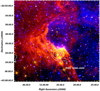 |
Fig. 1 Composite image of S169 and its environs showing the (IRAC-GLIMPSE) emissions at 8.0 (red) and 5.8 μm (green). The superCOSMOS Hα emission is in blue. White contours depict the continuum emission at 870 μm (ATLASGAL) arising from IRAS 12326-6245. |
Observational parameters for the observed transitions.
2 Observations and databases
2.1 Molecular observations
The molecular observations presented in this paper were made in December 2016 with the Atacama Pathfinder EXperiment1 (APEX) telescope (Güsten et al. 2006) at Llano de Chajnantor (Chilean Andes). As the front end for the observations, we used the APEX-1receiver of the Swedish Heterodyne Facility Instrument (SHeFI; Vassilev et al. 2008). The back end for all observationswas the eXtended bandwidth Fast Fourier Transform Spectrometer2 (XFFTS2), with a 2.5 GHz bandwidth divided into 32 768 channels. The observed transitions and basic observational parameters are summarized in Table 1. Calibration was done by the chopper-wheel technique and the output intensity scale given by the system is TA, which represents the antenna temperature corrected for atmospheric attenuation. The observed intensities were converted to the main-beam brightness temperature scale by Tmb = TA/ηmb, where ηmb is the main beam efficiency. For the APEX-1 receiver we adopted ηmb = 0.75.
Observations were made using the on-the-fly (OTF) mode with a step size of 10′′ (full sampling) in two orthogonal scan directions along RA and Dec (J2000). For the lines CO (2–1), 13 CO (2–1), and C18 O (2–1) the observed region was of ~14′ × 14′ in size centered on RA, Dec (J2000) = (12h 35m 44s, −63°00′08′′). For the lines HCN (3–2) and HCO+ (3–2) the observed region was ~4′ × 4′ in size centered on the position of the source IRAS 12326-6245 at RA, Dec (J2000) = (12h 35m 33s, −63°02′56′′). The data reduction was carried out with the CLASS90 package of the IRAM GILDAS software2.
2.2 Archival data
Infrared data
(a) Images of ATLASGAL at 870 μm (345 GHz) (Schuller et al. 2009). This survey covers the inner Galactic plane, l = 300° to 60°, |b| ≤ 1.°5, with the root mean square (rms) noise in the range of 0.05–0.07 Jy beam−1. The beam size at 870 μm is 19. ′′ 2. (b) Images from the Herschel3 Infrared GALactic (Hi-GAL) plane survey key program (Molinari et al. 2010). We used images from the photometric array camera and spectrometer (PACS) survey at 70 and 100 μm, with FWHM of 5. ′′5 and 11′′, respectively,and from the spectral and photometric imaging receiver (SPIRE) at 350 μm with a FHWM of 25′′. (c) Images from Spitzer at 5.8 and 8.0 μm from the Galactic Legacy Infrared Mid-Plane Survey Extraordinaire (Spitzer-GLIMPSE, Benjamin et al. 2003), retrieved from the Spitzer Science Center4. The images have a spatial resolution of ~2′′.
Radio continuum data
Mosaics obtained from the Sydney University Molonglo Sky Survey5 (SUMSS; Bock et al. 1999). This widefield radio imaging survey covers the southern sky at 843 MHz. The resolution is 43′′ × 43′′cosec(δ) and the rms noise level is ~1 mJy beam−1.
Hi data
Data cubes from the Southern Galactic Plane Survey (SGPS; McClure-Griffiths et al. 2005). This survey includes the regions limited by Galactic longitude 253° ≤ l ≤ 358° (SGPS-1) and 5° ≤ l ≤ 20° (SGPS-2) and Galactic latitude |b| ≤ 1. °5. Interferometric observations obtained with the Australia Telescope Compact Array (ATCA) are combined with single dish data from the 64 m Parkes radiotelescope. The final products have an angular resolution of ~2′ and a rms sensitivity of ~1 mJy beam−1.
Narrow band Hα data
Retrieved from the SuperCOSMOS Hα Survey6 (SHS). The images have a spatial resolution of ~1″ (Parker et al. 2005).
To investigate ionizing stars candidates and YSO candidates in the region of the nebula, we made use of the IRAS Point Source Catalog7 (Beichman et al. 1988), the MSX Infrared Point Source Catalog8 (Egan et al. 2003), the WISE All-Sky Source Catalog9 (Wright et al. 2010), the GLIMPSE point source catalog10 (Benjamin et al. 2003), the Two Micron All Sky Survey (2MASS)11 (Skrutskie et al. 2006), the American Association of Variable Star Observers (AAVSO) Photometric All-Sky SurveyA (APASS)12 (Henden et al. 2010), the ASCC-2.5 V3: All-sky Compiled Catalog of 2.5 million stars (Kharchenko & Roeser 2009), and the Astrometric catalog GAIA Data Release 2 13 (DR2; Gaia Collaboration 2016, 2018).
3 Molecular and dust emission
3.1 Emission of CO and its isotopologs
Figure 2 portrays the total averaged spectra of CO (2–1), 13 CO (2–1), and C18 O (2–1) in a region of ~14′ × 14′ in a positionthat is approximately at the center of the bubble nebula. The CO emission clearly depicts a strong narrow velocity component peaking at approximately −39 km s−1 and two weaker broad velocity components peaking at approximately −25 km s−1 and approximately −17 km s−1. For the sake of the analysis, these components will be hereafter referred to as component A, component B, and component C, respectively.
The peak velocity of component A, which is very likely dominated by the emission of IRAS 12326-6245, is almost coincident with the peak velocity of reported non-masing and masing emission lines towards the IRAS source (Bronfman et al. 1996; Zinchenko et al. 2000; Henning et al. 2000; Dedes et al. 2011; Araya et al. 2005; Caswell 1998, 2009; MacLeod et al. 1998). This component is also detected in 13 CO and C18 O emissions, which indicates that it is composed of high density molecular gas. Components B and C, on the other hand, are barely detected in the 13 CO emission and not detected in the C18O emission. As opposed to the case of the velocity of component A, neither masing nor non-masing emission lines were reported for IRAS 12326-6245 at the velocity of components B and C.
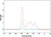 |
Fig. 2 Total averaged spectra of CO (2–1) (red), 13CO (2–1) (green), and C18 O (2–1) (blue) obtained within a region of ~14′ × 14′ centered on RA, Dec (J2000) = (12h 35m 44s, −63°00′08′′). |
3.2 Component A
In Fig. 3, we show the spatial distribution of the CO (2–1), 13 CO (2–1), and C18 O (2–1) lines in the velocity interval from approximately −42 to −37 km s−1. As expected according to the IR emission distribution (see Fig. 1), the bulk of the molecular emission appears concentrated toward the eastern and southern borders of the IR nebula, with no significant molecular emission detected toward the western and northeastern regions. The morphology and location of component A, Hα emission (see Fig. 1), and radio continuum emission (see Sect. 4) suggest that the ionized gas is expanding against the molecular cloud in the eastern and southern borders. The molecular emission at the southern border of the bubble seems to be tracing the densest areas, which are probably sculpted by the action of the HII region. The morphology and location of component A with respect to the near IR emission is similar to many other in Galactic IR bubbles found in the literature (e.g., Zavagno et al. 2006; Deharveng et al. 2008, 2009; Anderson et al. 2015; Liu et al. 2015; Cappa et al. 2016; Duronea et al. 2017; Devine et al. 2018). For a better visualization and comparison with the IR emission, in panel a of Fig. 4 we show the emission of 13 CO (2–1) of component A superimposed on the IRAC-GLIMPSE emissions at 8.0 and 5.8 μm.
From Fig. 3, it can also be seen that the CO emission of component A is more extended than that of 13 CO and C18 O. This indicates that 13 CO and C18 O lines, optically thinner than that of CO (see below), are actually tracing the distribution of the densest molecular gas surrounding the bubble nebula. In order to perform a more detailed analysis of the dense molecular gas in component A, we have roughly identified six molecular condensations in the 13 CO (2–1) emission using the C18 O (2–1) emission (which traces the denser gas) as a reference. The identification was done using the 1.5 K km s−1 contour level in the 13 CO (2–1) emission. The condensations are labeled in Fig. 3 as MC1, MC2, MC3, MC4, MC5, and MC6. These condensations are the places where star formation is likely to be taking place (see Sect. 5). In panels b to i of Fig. 4, we show the channel maps of 13 CO in the velocity range from −36.7 to −42.5 km s−1 in intervals of 0.7 km s−1. In order to compare the molecular emission distribution with the warm and cold dust emission, the 13 CO emission was superimposed on the 8.0 and 5.8 μm (IRAC-GLIMPSE) and the 870 μm (ATLASGAL) maps. Figure 4 shows that MC3, located at RA, Dec (J2000) = (12h 35m 35s, −63°02′25′′), is the only molecular condensation that is present in the entire velocity range. The position and size of MC3 perfectly match with those of the bright spot seen at 870 μm. This condensation certainly represents the carbon monoxide counterpart of IRAS 12326-6245, which reveals the physical association between S169 and the IRAS source. In the velocity interval from −36.7 to −38.2 km s−1 condensation MC1 becomes noticeable, reaching its peak temperature in the velocity interval from −38.9 to −39.6 km s−1, close to a 8.0 μm source seen at RA, Dec (J2000) = (12h 35m 24s, −63°05′42′′). It can be detected till a velocity of −40.4 km s−1. For the case of condensation MC2, it can be first noticed in the velocity interval from −36.7 to −38.9 km s−1, where its emission merges with MC1. Its peak emission is observed in the velocity range from −37.4 to −38.2 km s−1 and is coincident with another 8.0 μm source seen at RA, Dec (J2000) = (12h 35m 29s, −63°04′25′′). Condensation MC4 becomes detectable in the velocity interval from −36.7 to −37.4 km s−1, reaching to its maximum peak emission in the velocity interval from −38.2 to −38.9 km s−1. It can be noticed till a velocity of −39.6 km s−1 although its emission appears blended with MC2. Regarding condensations MC5 and MC6, they become detectable in the velocity range from −36.7 to −37.4 km s−1. Their emission distribution is quite irregular and achieve their peak temperatures in the velocity range from −38.2 to −38.9 km s−1. Condensation MC4 is detectable till a velocity of −39.6 km s−1, while MC5 till a velocity of −40.4 km s−1.
Figure 4 also shows a strong morphological correlation between the brightest parts of the PDR (described in Sect. 1) and the molecular condensations MC3, MC4, and MC5, especially at velocities between –38.2 and –38.9 km s−1. In particular, it is noticeable how the bright emission feature detected at 5.8 and 8.0 μm borders the area of MC3, which are likely to be exposed to stellar radiation.
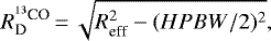
To estimate the physical properties of the 13CO condensations, we obtained six 13CO emission maps (not shown here) integrated in the velocity interval in which each condensation is detected. The deconvolved effective radius of the condensations derived from the 13 CO line,  , is calculated as:
 (1)
(1)
where Reff is the effective radii of the condensation (Reff =  ), being Acond the area of the condensation, and HPBW is the half-power beam width of the instrument. To estimate
  and other parameters, we adopted a distance of 2.03
 kpc (see Sect. 6.2). Then we obtained the effective radii of 0.40, 0.27, 0.94, 0.49, 0.75, and 0.86 pc for MC1, MC2, MC3, MC4, MC5, and MC6, respectively.
Assuming that all rotational levels are thermalized with the same excitation temperature (LTE) and that the emission is optically thick, we derived the excitation temperature of each molecular condensation, Texc, from the CO (2–1) line using
![Mathematical equation: \begin{equation*} T_{\textrm{peak}}\,{=}\,T_{12}^*\left[\left(e^{\frac{T_{12}^*} {T_{\textrm{exc}}}}-1\right)^{-1} -\left(e^{\frac{T_{12}^*} {T_{\textrm{bg}}}}-1\right)^{-1}\right],\end{equation*}](/articles/aa/full_html/2021/02/aa39074-20/aa39074-20-eq6.png) (2)
(2)
where  = hν12∕k, being ν12 the frequency of the 12CO(2–1) line, and Tbg = 2.7 K. To obtain the peak main beam temperatureof the CO (2–1), 13CO (2–1), and C18O (2–1) lines (Tpeak), we used Gaussian fits over the spectra profiles obtained integrating in the direction of the peak emission of the 13 CO condensations (in all the cases coincident with those of the C18O emission) over an area equivalent to the area of the beam. It is worth to point out that a single Gaussian component was considered for MC3, which shows self-absorption in the spectrum of CO (2–1) at the velocity of the peak emission of 13 CO (2–1) and C18 O (2–1) (Henning et al. 2000; Dedes et al. 2011). Excitation temperatures derived with Eq. (2) are then 21.3 K, 33.8 K, 47.8 K, 21.2 K, and 16.0 K, and 16.8 K for MC1, MC2, MC3, MC4, MC5, and MC6, respectively.
The optical depths (τ) of the 13CO (2–1) and C18 O (2–1) lines, denoted in the next equations as τ13 and τ18, respectively,were obtained assuming that the excitation temperature is the same for CO (2–1), 13 CO (2–1), and C18 O (2–1), and using the expressions
![Mathematical equation: \begin{equation*} \tau^{13}\,{=}\,{-}\textrm{ln}\left[1-\frac{T_{\textrm{peak}} {^{13}\textrm{CO}}}{T_{13}^*} \left[\left(e^{\frac{T_{13}^*} {T_{\textrm{exc}}}}-1 \right)^{-1}-\left(e^{\frac{T_{13}^*} {T_{\textrm{bg}}}}-1\right)^{-1}\right]^{-1}\right]\end{equation*}](/articles/aa/full_html/2021/02/aa39074-20/aa39074-20-eq8.png) (3)
(3)
and
![Mathematical equation: \begin{equation*} \tau^{18}\,{=}\,{-}\textrm{ln}\left[1-\frac{T_{\textrm{peak}} {C^{18}\textrm{O}}}{T_{18}^*} \left[\left(e^{\frac{T_{18}^*} {T_{\textrm{exc}}}}-1 \right)^{-1}-\left(e^{\frac{T_{18}^*} {T_{\textrm{bg}}}}-1\right)^{-1}\right]^{-1}\right],\end{equation*}](/articles/aa/full_html/2021/02/aa39074-20/aa39074-20-eq9.png) (4)
(4)
where  = hν13∕k,
  = hν18∕k, with ν13 and ν18 the frequencies of the 13CO (2–1) and C18 O (2–1) lines, respectively. We can also estimate the optical depth of the CO(2–1) line from the 13 CO(2–1) line using
![Mathematical equation: \begin{equation*} \tau^{12} \,{=}\,\ \left[\frac{\nu^{13}}{\nu^{12}} \right]^2\ \,{\times}\, \left[\frac{\Delta {v}^{13}} {\Delta {v}^{12}} \right]\ \,{\times}\, \left[\frac{\textrm{CO}}{^{13}\textrm{CO}} \right]\ \tau^{13},\end{equation*}](/articles/aa/full_html/2021/02/aa39074-20/aa39074-20-eq12.png) (5)
(5)
where CO/13CO is the isotope ratio (assumed to be ~62; Langer & Penzias 1993); Δv13 and Δv12 are defined as the full width half maximum (FWHM) of the spectra of the 13 CO and CO lines, respectively, which are derived by using a single Gaussian fitting (FWHM = 2 ×  × σgauss).
In LTE, the 13CO and C18 O column densities can be estimated from the 13CO (2–1) and C18 O (2–1) line using
![Mathematical equation: \begin{equation*} N({^{13}\textrm{CO}})\,{=}\,3.23\,{\times}\, 10^{14} \left[\frac{e^{ \frac{T_{13}^*}{T_{\textrm{exc}}} }}{1 -e^{- \frac{T_{13}^*}{T_{\textrm{exc}}} } }\right] T_{\textrm{exc}} \int \tau^{13}\ \textrm{d}v \ \ \textrm{ (cm$^{-2}$)}\end{equation*}](/articles/aa/full_html/2021/02/aa39074-20/aa39074-20-eq14.png) (6)
(6)
and
![Mathematical equation: \begin{equation*} N({\textrm{C}^{18}\textrm{O}})\,{=}\,3.21\,{\times}\, 10^{14} \left[\frac{e^{ \frac{T_{18}^*}{T_{\textrm{exc}}} }}{1 -e^{- \frac{T_{18}^*}{T_{\textrm{exc}}} } }\right] T_{\textrm{exc}} \int \tau^{18}\ \textrm{d}v \ \ \textrm{ (cm$^{-2}$)}.\end{equation*}](/articles/aa/full_html/2021/02/aa39074-20/aa39074-20-eq15.png) (7)
(7)
The integral in Eqs. (6) and (7) can be approximated by
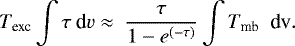 (8)
(8)
This approximation helps to eliminate to some extent optical depth effects and is good within 15% for τ < 2 (Rohlfs & Wilson 2004). Bearing in mind the values of τ13 obtained, the approximation is appropriate for our region. Estimations of the H2 column density, N(H2), were obtained from both the 13CO and C18 O column densities, and adopting abundances X[13CO] = 7.1 × 10⁵ and X[C18O] = 5.9 × 10⁶ (Frerking et al. 1982). For the optical depth and column density, we estimated uncertainties of about 20 and 25%, respectively, arising mostly from calibration uncertainties of about 20% (Dumke & Mac-Auliffe 2010).
The total hydrogen mass of each clump was calculated using
 (9)
(9)
where msun is the solar mass (~2 × 1033 g), μ is the mean molecular weight, which is assumed to be equal to 2.76 after allowing for a relative helium abundance of 25% by mass (Yamaguchi et al. 1999), mH is the hydrogen atom mass (~1.67 × 10⁻²⁴ g), Ω is the solid angle of the 13 CO emission expressed in sr, d is the adopted distance expressed in cm, and N(H2) is the H2 column density obtained from  . Uncertainties in molecular masses are about 60%, and originate mainly from a distance uncertainty of about 30% (see Sect. 6.2). The derived physical parameters are presented in Table 2.
In order to perform a study of the molecular gas in IRAS 12326-6245, we also present an analysis for MC3 using the high-density tracer lines HCN (3–2) and HCO+ (3–2). In Fig. 5, we show the emission of these lines in the velocity intervals from −47.6 to −29.2 km s−1 and −44.8 to −32.5 km s−1, respectively. Their emissions show a good morphological correspondence with that at 870 μm (see Fig. 4) and seem to be delineating an obscured region in the 8.0 and 5.8 μm emissions. They are certainly the HCN and HCO+ counterparts of the molecular condensation MC3. In order to estimate the HCN and HCO+ column densities, we used LTE models numerically approximated with the Markov chain Monte Carlo (MCMC) method (Foreman-Mackey et al. 2013). The lines in LTE were simulated and compared with the observations (e.g., Comito et al. 2005; Möller et al. 2017). The solutions presented were obtained from the averaged spectra considering different offsets since the individual solutions for each one of them were similar. That is a consequence of the homogeneous emission traced by the species analyzed here. In Fig. 5, we show the average spectra (in antenna temperature) of HCN (3–2) and HCO+ (3–2). The results presented here were obtained by taking into account those reported in IRAS 12326-6245 by Dedes et al. (2011), who assumed temperature values of 150 and 50 K for the gas conditions of species in an apparent hot core region and extended envelope, respectively. For the sake of the analysis, we also included the optically thin lines of 13 CO (2–1) and C18 O (2–1). Then, assuming an excitation temperatureof Texc = 50 K for the HCO+ (3–2) line, we obtained a column density of N(HCO+) = (5.2 ± 0.1) × 1013 cm−2. For the 13CO (2–1) and C18 O (2–1) lines, also adopting Texc = 50 K, we obtained N(13CO) = (2.01 ± 0.04) × 1017 cm−2 and N(C18O) = (3.9 ± 0.1) × 1016 cm−2. For the case of the HCN (3–2) line, LTE models suggest a physical condition related with the hot core region. Based on the hypothesis stating that Texc = 150 K, we derived N(HCN) = (1.9 ± 0.5) × 1014 cm−2. Concerning the uncertainties, the results presented here are approximations that should be considered (at least) within the calibration uncertainty since several assumptions were adopted for single transitions. In order to inspect the quality of the fits, in Fig. 5 we also exhibit the residuals after subtracting the emission lines from their LTE models.
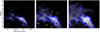 |
Fig. 3 Spatial distribution of the C18O(2–1) emission (left panel), 13CO(2–1) emission (middle panel), and CO(2–1) emission (right panel) in the velocity interval from approximately −42 to –37 km s−1 (component A). In the left panel, the contours are 0.35 (~3 rms), 0.7, 1.15, 2, 3, 5, and 7 K km s−1. In the middle panel the contour levels are 0.5 (~6 rms), 1, 1.5, 2, 2.5, 3, 4, 5, 7, 9, 11, 13, and 15 K km s−1. In the right panel the contour levels are 1.5 (~20 rms), 2, 2.5, 3, 4, 5, 6, 8, 10, 14, 18, 22, and 26 K km s−1 (Tmb). Identified molecular condensations are indicated in yellow over the 13CO (2–1) emission. |
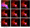 |
Fig. 4 Panel a: emission distribution of the 13CO(2–1) line in the total velocity range from –37 to –42 km s−1 (white contours and blue color scale) superimposed on the IRAC-GLIMPSE images at 8.0 and 5.8 μm (red and green color scales, respectively). The contours levels are the same than those shown in the middle panel of Fig. 3. Panels b to i: channel maps of the 13 CO (2–1) line emission in velocity intervals of 0.7 km s−1 (white contours) in the velocity range from –36.7 to –42.5 km s−1 superimposed on the 8.0 and 5.8 μm (IRAC-GLIMPSE) emissions (red and green color scales) and 870 μm ATLASGAL emission (blue color scale) inside the 3 rms limit. Contours levels are 0.9 (~5.5 rms), 2.6, 4.4, 6.2, 7.9, 10, 12, 16, and 20 K km s−1. The velocityinterval is indicated in the top right corner of each panel. |
Observed parameters obtained from the emission lines and physical properties derived for the molecular condensations MC1 to MC6.
3.3 Components B and C
As mentioned in Sect. 3.1, two weaker broad velocity molecular components peaking approximately at −25 km s−1 (component B) and −17 km s−1 (component C) were also detected in S169. These components are hardly detected in the 13 CO emission and not detected at all in the C18O emission, which certainly indicates that they are mostly composed by low-density gas. In order to analyze their spatial distribution, we constructed two CO emission maps integrated in the velocity intervals from −28.9 to −18.9 km s−1 (component B) and from−18.2 to −12.7 km s−1 (component C). They are shown in Fig. 6 superimposed onto the 8.0 and 5.8 μm emissions. For the case of component B, three molecular features are seen projected towards different regions of the nebula. The brightest feature (hereafter, feature 1) is seen approximately centered at RA, Dec (J2000) = (12h 36m 34s, −62°55′13′′) perfectly delineating the northeastern and northern borders of the IR nebula. As can be seen from the figure, the brightest regions of the molecular gas appear projected onto the faintest regions of the IR emission, which suggests that a PDR was formed over the surface of feature 1 (viewed from the side). Another feature is seen centered approximately at RA, Dec (J2000) = (12h 36m 40s, −63°06′00′′) (feature 2). This feature appears bordering the southeastern edge of the nebula, also projected onto the faintest regions of the IR nebula. The third feature is seen projected along the center of the nebula approximately at Dec = −62°58′00′′ and is still noticeable at more negative velocities. Since this feature shows no morphological correspondence with any region of the IR nebula, a physical link with S169 cannot be suggested. Probably, it is an unconnected molecular structure located behind the nebula since no absorption features can be noticed along the brightest regions of the IR emission. Regarding component C, only one molecular structure (feature 3) stands out, peaking approximately at RA, Dec (J2000) = (12h 35m 05s, −62°58′00′′). This feature shows a good morphological correspondence with the faint IR arclike filament seen at the western section of the nebula at RA = 12h 35m 10s. This correspondence is also well-displayed in Fig. 10. Another structure has been noted at the northeastern region of the nebula, however it represents the remains of feature 1 at slightly more positive velocities.
Since no discernible emission of the 13CO (2–1) line is detected for features 1, 2, and 3, in order to estimate their column density and mass, we use the relation between the H2 integrated column density and the CO integrated emission:
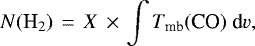 (10)
(10)
where X is an empirical factor that has been shown to be roughly constant for the 12 CO(1–0) line in Galactic molecular clouds and lies in the range of (1–3) × 1020 cm−2 (K km s−1)−1, as estimatedby the virial theorem and γ-ray emission (Bloemen et al. 1986; Solomon et al. 1987; Digel et al. 1996; Strong & Mattox 1996). In this paper, we adopt X = 1.6 × 1020 cm−2 (K km s−1)−1 (Hunter et al. 1997). The integrated emission ∫ Tmb(CO) dv was calculated adopting an area determined by the first contour level indicated in Fig. 6. For the column density, we estimated an uncertainty of about 50%, arising mostly from the factor X and calibration uncertainties. The mass of the features were then estimated using Eq. (9). The obtained parameters are shown in Table 3. It is worthwhile to point out that the area and mass obtained for features 1 and 2 are likely lower limits since these features seem to be part of a larger structure (extending beyond the area covered in our APEX observations), which probably corresponds to the parental molecular cloud in which the IR bubble was formed.
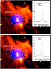 |
Fig. 5 Upper panel: spectral line and LTE model of the HCN (3–2) line obtained from LTE-MCMC calculations assuming Texc = 150 K (see text), with a resulting density of N = (1.9 ± 0.5) × 1014 cm−2. The blue line indicates the residual obtained from the subtraction between the observation and LTE model. In colors: spatial distribution of the HCN (3–2) emission in the velocity interval from −47.6 to −29.2 km s−1 (color blue and white contours) superimposed on the IRAC 8 and 5.8 μm emissions (red and green colors). Lower panel: same as above for the HCO+ (3–2) line, assuming Texc = 50 K, with a resulting density of N = (5.2 ± 0.1) × 1013 cm−2. The HCO+ (3–2) emission distribution is in the velocity interval from −44.8 to −32.5 km s−1. The contour levels for the HCN (3–2) are 0.25 (~5 rms), 0.85, 2.2, and 4.0 K km s−1; and for the HCO+ (3–2) line, they are 0.28(~5 rms), 0.8, 2.4, and 5 K km s−1 |
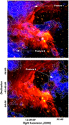 |
Fig. 6 Upper panel: spatial distribution of the CO emission (blue color scale and white contours) in the velocity interval from −28.9 km s−1 to −18.9 km s−1 (component B) superimposed on the IRAC 8 μm and 5.8 μm emissions (red and green color scales). The contour levels start from 0.95 K km s−1 (~9 rms) in stepsof 0.5 K km s−1. Lower panel: spatial distribution of the CO emission in the velocity interval from −18.2 to −12.7 km s−1 (component C). The contour levels start from 0.85 K km s−1 (~7 rms) in stepsof 0.4 K km s−1. |
Physical properties estimated for the CO feature 1, feature 2, and feature 3.
3.4 Submillimeter dust emission
In the upper panel of Fig. 7, we present a three-color composite image of S169 as seen by Herschel images. The 70 and 160 μm emissions (red and green color scales, respectively) underline the emission of the warmer dust close to the ionized gas. As can be seen from the figure, the emission at 70 μm has a good morphological correspondence with the IRAC 8 μm emission (black contours), although the latter exhibits a sharper edge towards the center of the nebula (see also Fig. 1), which is likely due to the destruction of the PAH molecules by the ionization front. The 70 μm emission, in contrast, is more diffuse (partly because of the lower angular resolution) and extends towards the center of the nebula, which indicates that it is also tracing the warm dust that still remains mixed with the ionized gas. The same feature can be observed in the IRAC-GLIMPSE 24 μm emission (not shown here). The 350 μm emission (blue color scale) seems to be underlining the emission from the dust in the outer parts of the nebula. It is very likely that the emission distribution at this wavelength is mostly tracing the distribution of the cold dust immersed in the parental molecular cloud placed at the eastern border of the nebula, which is partially disclosed by features 1 and 2 (see Fig. 6).
To study the distribution of the dust temperature in the nebula, we constructed a temperature map from the ratio of the observed fluxes in two Herschel bands. Since a high level of radiative feedback from powering massive stars is usually observed in HII regions/IR bubbles, it is reasonable to assume that the molecular gas and dust are not too cold. Then we used the ratio of the 70 versus 160 μm maps, which are better suited to measure color temperatures up to ~80 K. Furthermore, the angular resolution of the temperature map obtained using these bands is the highest resolution achievable from the Herschel maps. The 70 μm map was smoothed down to the angular resolution of the 160 μm data. Then the temperature map was constructed as the inverse function of the ratio 70–160 μm maps that is,  . Assuming a dust emissivity following a power law of κν ∝νβ, with β as the spectral index of the thermal dust emission (assumed to be β = 2), in the optically thin thermal dust emission regime, f(T) takes the parametric form:
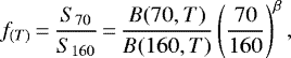 (11)
(11)
where B(70, T) and B(160, T) make up the blackbody Planck function for a temperature T at wavelengths 70 and 160 μm, respectively. The assumption that the emission is optically thin is further justified from the derived column densities in the nebula (see Preibisch et al. 2012 for details). From the obtained map (middle panel of Fig. 7), dust temperatures between ~20 and 30 K can be discerned. These temperatures are commonly observed in the closest regions of IR bubble nebulae (e.g., Anderson et al. 2012; Duronea et al. 2015; Figueira et al. 2017). Warmer dust is seen in the region of the denser molecular condensations (MC1, MC2, MC3, and MC4) and the border of the PDR, particularly on two spots at RA, Dec (J2000) = (12h 35m 24s, −63°00′56′′) and RA, Dec (J2000) = (12h 35m 35s, −63°02′29′′) where the temperature achieves ~30 K. The first spot is coincident with a bright rim placed over the southern region of the PDR and a peak in the radio continuum emission (see Fig. 8 in Sect. 4), which suggests external heating of the dust. The second spot is coincident with the molecular condensation MC3 (IRAS12326-6245) which is very likely to indicate that the dust is also internally heated. Not surprisingly, lower temperatures (12–18 K) are seen in the region of feature 3 and behind the PDR, coincident with the position of features 1 and 2.
With the temperature map, we converted the surface brightness map at 160 μm into a beam averaged column density map using (Hildebrand 1983):
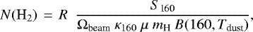 (12)
(12)
where Ωbeam is the beam solid angle (π  / 4 ln 2), R is the gas-to-dust ratio (assumed to be 100), and κ160 is the dust opacity per unit mass at 160 μm assumed to be 40.5 cm2 g−1 (Ossenkopf & Henning 1994). The resulting map (presented in the lower panel of Fig. 7) gives an overall view of the density distribution in the whole region of the nebula. Clearly, denser regions are observed behind the PDR in the region of component A, especially towards IRAS12326-6245, where the column density achieves peak values up to ~4 × 1022 cm−2.
As shown in Figs. 1 and 4, the source IRAS 12326-6245 is very bright in the continuum emission at 870 μm (no emission at this wavelength is detected above the 3 rms limit outside the IRAS source). The emission at 870 μm is usually optically thin and dominated by the thermal emission from dust contained in dense material (e.g., dense molecular cores or filaments). Then we used the image of ATLASGAL to more confidently derive the beam averaged density in IRAS 12326-6245 using Eq. (12). For the calculations, we adopted κ870 = 1.85 cm2 g−1, a value that is representative for relatively dense molecular clouds (Ossenkopf & Henning 1994; Henning et al. 1995) and Tdust = 30 K and we obtained a column density of N(H2) = 8.2 × 1023 cm−2. This value is almost two orders of magnitude higher than that observed in the column density map obtained with the emission at 160 μm, which might indicate that the emission is optically thick at that wavelength. Furthermore, the temperature used to derive N(H2) in IRAS 12326-6245 (30 K) might have been underestimated since, as mentioned above, its emission at 160 μm might not be optically thin at such high density. This could led to an overestimation of the column density in the IRAS source. The column density obtained from the 870 μm emission is also somewhat higher than those derived for MC3 in Sect. 3.2 from the 13 CO (2–1) and C18 O (2–1) emissions. We do keep in mind, however, that the column density values derived from continuum IR and carbon monoxide emissions are strongly dependent on the adopted abundances (dust and carbon monoxide-to H2).
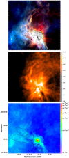 |
Fig. 7 Upper panel: three-color composite image of S169: Herschel PACS 70 and 160 μm emission are in red and green, respectively. Herschel SPIRE 350 μm emission is in blue. Black contours underline de IRAC-GLIMPSE 8 μm emission at 35, 55, 75, 105, 150, 170, 300, and 500 MJy sr−1. Middle panel: dust temperature map derived from the 70 and 160 μm emission. The color temperature scale is on the right. Lower panel: column density map obtained from the 160 μm emission. Dashed black contours indicate the location of molecular concentrations MC1 to MC6 for orientation. |
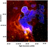 |
Fig. 8 Radio continuum emission distribution at 843 MHz (blue color and white contours), superimposed on the 8 and 5.8 μm emission (red and green color). Contours levels are 3.1 (~3 rms), 4.5, 6.3, 7.6, 12, 20, 30, 40, 100, 200, 300, and 400 mJy beam−1. |
4 Ionized gas
In Fig. 8, we show the radio continuum emission map at 843 MHz overlaid on the 8.0 and 5.8 μm emissions. Three bright structures stand out in the direction of the nebula. The brightest one (S843 = 985 mJy), which does not have a discerniblecounterpart in the Hα emission, is observed towards the norther border of the nebula at RA, Dec (J2000) = (12h 35m 39s, −62°54′26′′). Using a radio continuum image from the SGPS (not shown here), we found that this compact source has an integrated flux density of S1384 = 0.63 mJy. Since the spectral index turns out to be α = −0.9, we conclude that this source is extragalactic and will not be taken into further consideration.
An arc-shaped structure can be discerned towards the center of the nebula, which may be described by two main components: (i) a southern bright component with its outer edge closely delineating the PDR depicted by the 8.0 μm emission; and (ii) a weaker tail about 5′-long extending from the northern end of the previous component towards the northwest. A number of artifacts in the radio continuum emission areobviously produced by sidelobes and grating rings from the bright extragalactic source, such as a void at RA, Dec (J2000) ≈ (12h 35m 45s, −62°56′33′′) and two radial strips connecting the compact source and the weak tail. Hence, we believe that the morphology of the arc-shaped structure is probably distorted in the region closer to the extragalactic source. However, the morphology of the unaffected part (southernmost component) suggests that the ionized gas traced by the radio continuum emission is likely to be expanding against component A and features 1 and 2, supporting the same conclusion derived in Sect. 1 based on the Hα emission.
Using the integrated radio continuum flux obtained for the whole arc-shaped structure (i.e., the southern bright component and weaker tail), S843 = 308 mJy, we obtained its electron density and ionized mass using (Panagia & Walmsley 1978):
 (13)
(13)
and
 (14)
(14)
where Te is the electron temperature (assumed to be 1 × 10⁴ K) in units of 104 K, θR is the angular radius of the source in arc minutes (assumed to be 4′), b(ν, Te) = 1 + 0.3195 × log(Te/ 104 K) – 0.213 × log(ν/1 GHz), d is in kpc, and Y is the abundance ratio by number of He+ to H+. Then we obtained ne = 15 cm−3 and Mion = 17 M⊙. It is worthwhile pointing out that the presence of the extragalactic source projected on S169 prevents the estimation of the whole radio continuum emission related to the structure.
The number of ionizing Lyman continuum photons needed to sustain the current level of ionization in the arc-shaped structure can be calculated using (Chaisson 1976):
 (15)
(15)
where Te is in units of 104 K, S843 is in Jy, ν is in GHz, and d is in kpc. Then, in considering distance uncertainties, we obtained for this source a range of NLyc = 0.5–2.0 × 1047 s−1. We keep in mind that these values are likely lower limits since about 25–50% of the UV photons are absorbed by interstellar dust in the HII region (Inoue 2001). Furthermore, Watson et al. (2008), on the basis of studies of several bubbles, concluded that NLyc estimated with this method is lower than expected by about a factor of 2. Then for the arc-shaped structure, we estimate a range of NLyc ≈ (1–4) × 1047 s−1. Adopting ionizing photon rates extracted from Martins et al. (2005), we estimate the spectral type of the ionizing star of S169 to be at most O9.5V. Alternatively, a handful of later B-type stars could also be responsible for powering the HII region. The third structure detected in the 843 MHz emission is a small bright spot discernible in the southern region of the nebula at RA, Dec (J2000) = (12h 35m 35s, −63°02′29′′), which is certainly the radio continuum counterpart of IRAS 12326-6245. Using the flux density obtained for this source (S843 = 12 mJy), we obtained ne = 70 cm−3, Mion = 0.3 M⊙, and NLyc = (0.4–1.4) × 1046 s−1. It is worthwhile pointing out that for the previous estimations, we assumed optically thin emission at 843 MHz; since that assumption cannot be verified, estimations obtained with the Eqs. (13)–(15) should be taken as the lower limits. In fact, for the case of the radio continuum emission associated with IRAS 12326-6245, Dedes et al. (2011) used cm observations obtained by Urquhart et al. (2007) to derive a Lyman continuum flux of 8.2 × 1048 s−1, which is almost three orders of magnitude larger than the value obtained with Eq. (15) for the source.
In a broad sense, the distribution of the ionized gas inside the cavity suggests an electron density gradient, with the densest material near the border of the IR nebula. This configuration suggests that the nebula is bounded by density to the west, and bounded by ionization to the east, north, and south. Furthermore, the structure detected to the west of the nebula along RA ~12h 34m 44s, which appears connected with the eastern arc-shaped structure within the 3 rms emission limit, might be indicative of a “champagne-flow” scenario (Tenorio-Tagle 1979).
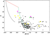 |
Fig. 9 Color magnitude diagram of stars searched in a region centered in S169. Black dots are young spectral type stars with different reddening values (see text in Sect. 5). Magenta, green, and yellow crosses represent the O9V, B1V, and B2V (or later) stars, all of them ionizing candidate stars displayed with the same colors in Fig. 10. Green and black curves represent the MS shifted according to the distance modulus adopted with and without reddening, respectively. Red line indicates the normal reddening path (Rv = 3.1). |
5 Stellar and protostellar content in the nebula
5.1 Ionizing star candidates
With the aim of identifying possible ionizing stars in the nebula, we first inspected IR catalogs in a region of ~7′ in radius centered on RA, Dec (J2000) ≈ (12h 35m 28s, −62°58′04′′). Making use of GLIMPSE data, we identified Class III candidates, which are usually referred to as main-sequence (MS) young stars using color-color diagrams (Allen et al. 2004). Then we cross-correlated these sources with sources selected from the 2MASS catalog with photometric uncertainty, Ks < 0.05 mag (Ducati et al. 2001), and we obtained ~600 Class III sources with reliable JHK photometry.Since none of these sources were found to have spectral classification, we used the parameter QNIR = (J−H) − 1.7(H−Ks) following Borissova et al. (2011) to separate sources between early (O–B) MS stars (−0.1 < QNIR <0.15) and stars that reveal IR excess (QNIR < –0.1) and are likely preMS stars or YSOs, or both. Then we obtained 60 MS candidates.
Next, we inspected visual catalogs in the same region. A search in the APASS and ASCC-2.5 V3 catalogs yielded 228 and 10 sources, respectively, both with V and B magnitudes. We also carried out a search in the astrometric catalog Gaia DR2 of more than 6000 sources with parallax data in the region of S169. Thereafter, we cross-correlated all sources found with the APASS, Gaia DR2, and ASCC-2.5 catalogs, obtaining only 90 sources in common between the first two catalogs, which includes the 10 sources of the ASCC-2.5 catalog. We then estimated the distance of visual sources employing the color-magnitude (B−V vs. V) diagram (see Fig. 9), calibrated with the optical (BV) (Schmidt-Kaler Th. 1982) to adjust the theoretical MS by a distance of ~2 kpc (see Sect. 6.2) and color excess E(B−V) = 0.8 magnitudes. Thus, we were able to identify the stars with photometric distance close to the nebula. Among these sources, only 19 had distances between 1.7 and 2.3 kpc that were estimated from the parallax catalog from Gaia.
In the next step, we cross-correlated the 60 MS candidates obtained from the IR data with the sources previously studied with a color magnitude diagram and we found 47 sources in common. In order to better determine their spectral types, we inspected their loci in a (J−H) vs. (H−K) diagram adopting the MS calibration given by Schmidt-Kaler (Th. 1982), Cousins (1978), and Koornneef (1983), the absorption ratios (rx = Ax∕Av) given by Rieke & Lebofsky (1985), van der Hulst curve 15, and the color transformations from 2MASS to Koorneef data of Carpenter et al. (2001).
Finally, we kept only those stars that are projected onto the cavity of the bubble (~3′ in radius centered on RA, Dec (J2000) ≈ (12h 35m 28s, −62°58′04′′)). This yielded only 10 sources with spectral types O9 (2 sources), B1 (1 source) and B2 or later (7 sources), all of them probable MS stars; it is worthwhile pointing out that only 5 of these sources belong to the group of 19 sources with distances between 1.7 and 2.3 kpc obtained from Gaia. The positions of these sources in the MC diagram and in the cavity are shown in Figs. 9 and 10, respectively.
5.2 Identification of candidate YSOs
Making use of the MSX, WISE and Spitzer point source catalogs, we look for the primary tracers of stellar formation activity onto the molecular clouds related to S169.
To thisaim, MSX sources were selected satisfying a flux quality Q > 1 in the four bands. WISE sources with photometric flux uncertainties >0.2 mag and signal-to-noise ratio (S/N) < 7 in the W1, W2, W3, and W4 bands, were rejected. Finally, we kept Spitzer sources with photometric uncertainties <0.2 mag in the four IRAC bands. Then, within a 14′ box centered at RA, Dec (J2000) = (12h 35m 44s, −63°00′08′′), we found a total of 2 MSX, 400 WISE, and 810 Spitzer sources fulfilling the selection criteria mentioned above. To identify candidate YSOs we adopted the classification scheme described in Lumsden et al. (2002), Koenig et al. (2012), and Gutermuth et al. (2009) for the MSX, WISE, and Spitzer sources, respectively. Several sources were found to qualify the above criteria, which are listed in Table A.1. The table presents the designation of the sources, their coordinates, flux densities, information concerning the type of the protostellar object, matching with another source in the table, and coincidence with a molecular or IR structure.
Among the MSX sources, we found one MYSO candidate, which coincides with the center of IRAS 12326-6245, and one CHII region candidate, which coincides with a WISE Class II candidate (see below). Before attempting to identify the candidate YSOs from the listed WISE and Spitzer sources, we selected the non-YSO sources with excess infrared emission, such as PAH emitting galaxies, broad line active galactic nuclei (AGNs), unresolved knots of shock emission, and PAH emission features. Then, a total of 89 and 51 WISE and Spitzer sources, respectively, were dropped from the lists. Among the remaining 311 WISE and 759 Spitzer sources, 12 (5 WISE and 7 Spitzer) were identified as Class I sources (i.e., sources with IR emission arising mainly from a dense infalling envelope, including flat spectrum objects) and 60 (43 WISE and 17 Spitzer) as Class II sources (i.e., preMS stars with optically thick disks).
The location of the identified candidate YSOs is shown in Fig. 10, where the 8.0 and 5.8 μm emissions together with the emissionof both the 13CO and CO structures (i.e, component A and features 1, 2, and 3) are also displayed. As expected, the bulk of the candidate YSOs are seen projected onto the densest molecular gas (component A). A noticeable feature is the concentration of sources along the two brightest PDR areas which, as mentioned in Sect. 3.2, delineates the borders of the molecular condensations. Namely, the WISE sources #5, #23, #24, #25, #27, #28, #29, #30, #32, and #35 to #47, seem to be related to the PDR closer to the ionized gas bordering the molecular emission of MC3 and MC4 (noted as (+) in the last column of Table A.1), while WISE sources #7, #18, #19, #20, #21, #22, and #26, and Spitzer sources #54, #65, #67, #68, and #69 lie along the PDR that lies farther away from the ionized gas and related to the densest parts of MC3, MC4, and MC5 (noted as (*) in Table A.1). Not surprisingly, another appreciable concentration of candidate YSOs, namely WISE sources #3, #6, #10, #11, #12, and #13, Spitzer sources #58, #59, #60, #66, and #71, and MSX sources #1 and #2 can be noticed in the region of the molecular concentration MC3.
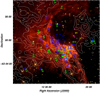 |
Fig. 10 MSX, WISE, and Spitzer candidate YSOs projected onto the IRAC-GLIMPSE image at 8.0 and 5.8 μm. Cyan diamonds indicate the MSX sources, blue circles and blue squares indicate WISE Class I and Class II sources, respectively, and green circles and green squares indicate the Spitzer Class I and Class II sources, respectively. The numerical references of YSOs are based on those from Table A.1. The size of the symbols do not necessary match the angular size of the sources. Ionizing candidate stars identified in Sect 5.1 are also indicated by crosses in magenta (O9V), green (B1V), and yellow (B2V or later). White contours indicate the 13 CO emission of component A (first contour level ~8 rms) and theCO emission of feature 1 (first contour level ~13 rms), feature 2 (first contour level ~12 rms), and feature 3 (first contour level ~10 rms). |
6 Discussion
6.1 A model for S169 and its molecular environment
Since IR bubbles are believed to be born within dense molecular clouds, the classical scenario predicts that, in a uniform medium, the molecular gas around the bubble should expand spherically. Under that assumption, a molecular shell with a central velocity V0 and an expansion velocity Vexp should depict in a position-position diagram a “disk-ring” pattern when observed at different velocities. At V0 (corresponding to the systemic velocity of the bubble), the shell should attain its maximum diameter; whereas, at extreme velocities (either negative or positive with respectto V0), the molecular emission should resemble a disk. At intermediate velocities, the radius of the ring shrinks as the extreme velocity is approached. Although these features were never observed all together in the molecular gas around IR bubbles, the behavior of the molecular gas around S169 certainly clashes with that of the classical IR bubble model.
In order to address the observed characteristics of the molecular gas associated with S169, we present a simple model taking into account its morphology, relative position with respect to the IR and Hα emissions and the velocity intervals as constraints. Needless to say, we assume that component A, feature 1, feature 2, and feature 3 are physically associated with S169, a well-grounded conclusion given their good morphological correspondence with the IR nebula.
Hence, we propose that component A and features 1, 2, and 3 could be explained in terms of an expanding, partially complete semispherical structure. A simple sketch is presented in Fig. 11, where the right ascension axis is indicated for the sake of clarity (the declination axis is then perpendicular to the sketch, increasing towards the reader). The expansion of the molecular gas is then revealed by the velocity of the different molecular structures. The molecular gas approaching in the direction of Earth is depicted by the molecular structure at more negative velocity (component A) with an approaching velocity of Vappr ≈ −39 km s−1, while the molecular gas receding is depicted by the structure at more positive velocity (feature 3) with a receding velocity of Vrec ≈ −17 km s−1. Molecular structures at intermediate velocities (features 1 and 2) thus represent the molecular gas at V0 ≈ −25 km s−1 expanding approximately in perpendicular directions with respect to the direction of Earth. A glance at Fig. 6 suggests that the expansion velocity of features 1 and 2 might have components in the direction of the declination axis, which is positive for the case of feature 1 and negative for the case of feature 2 (this cannot be depicted in the two-dimension sketch presented in Fig. 11).
Therefore, with this simple model we are able to explain not only the morphology and kinematics of the molecular gas, but also the characteristics of the ionized gas (traced by the radio continuum emission), which seems to be expanding against the molecular gas towards the east, north, and south, while it is expanding freely to the west, probably in a sort of a champagne-flow effect.
According to the model, a rough estimation of the expansion velocity of the molecular gas around S169 may be simply obtained by:
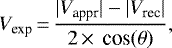 (16)
(16)
with θ as the angle between the line of sight and the direction of Vexp of component A and feature 2. Based on the morphology of the IR nebula, a conservative value θ = 25° can be adopted, and the obtained expansion velocity turns out to be Vexp ~12 km s−1. Having the expansion velocity, the dynamical age of the nebula, tdyn, can be derived considering a radius of 2.3 ± 0.8 pc (~4′ at a distance of 2.03 kpc), which turns out to be in the range of (1.2–2.6) × 105 yr.
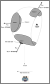 |
Fig. 11 Simple sketch of the proposed model to explain the morphology and velocity of the molecular gas associated with S169. The right ascension axis, as visualized by the observer, is indicated as reference (the declination axis is perpendicular to the planeof the sketch, increasing towards the reader). |
6.2 Distance to S169 and IRAS 12326-6245
As noted in Sect. 1, the adopted distance in the literature for IRAS 12326-6245 is 4.4 kpc. This value was first estimated by Osterloh et al. (1997), who performed a study of a number of southern IRAS sources using IR continuum and millimeter line data. The authors adopted distances that were taken from the literature where possible (either directly or by kinematic and spatial association with another source of known distance). Otherwise, kinematical distances were determined using the central velocity of the CS(2–1) or CO(2–1) emission lines and the Galactic rotation curve of Clemens (1985). For the case of IRAS 12326-6245, a kinematical distance could not be determined by the authors since the central velocity of the CS and CO lines (−39.4 km s−1 and −39.7 km s−1, respectively) are forbidden according to the Galactic rotation model. Then the authors adopted for IRAS 12326-6245 the distance to the source IRAS 1283-6128 (4.4 kpc), which is kinematically close to within 0.5 km s−1 as well as spatially to within 2°.
In Sect. 3.1, we offer a confirmation of the physical association between S169 and IRAS 12326-6245. Furthermore, according to the model proposed in Sect. 6.1, the source IRAS12326-6245 (embedded in component A) is expanding at a velocity coarsely estimated as Vexp ~ 12 km s−1 with respect to the systemic velocity of the bubble (V0 ≈−25 km s−1). Assuming that our model is well-suited to explain the characteristics of the molecular gas around the bubble nebula, this leads to the unavoidable conclusion that the velocity reported in the literature for IRAS 12326-6245 (approximately −39 km s−1) does not represent the velocity of the ISM in the surroundings of both, the IRAS source and S169. This is understandable considering that previous studies of IRAS 12326-6245 were not performed in the whole context of the nebula S169, but rather focused only on the IRAS source. Instead, we believe that the velocity of features 1 and 2 (approximately −25 km s−1), corresponding approximately to the systemic velocity of the bubble nebula, is more suitable for determining the kinematical distance for both, S169 and IRAS 12326-6245. Furthermore, in a study of the rotation curve in the Southern Galaxy, Alvarez et al. (1990) found an excess anomally of +12.2 km s−1 in the terminal velocities in the Galactic longitude range between l = 280 and l = 312, with respect to the trend in the rest of the IV Galactic quadrant. This excess includes the region studied here since we have our source at Galactic coordinates (l, b) = (301.134, –0.225). Next, by adopting a velocity of −25 km s−1, and using the rotation curve of Reid et al. (2014) with the Monte Carlo method14 (see Wenger et al. 2018 for details) and a conservative velocity uncertainty of 1 km s−1, two kinematical distances are obtained, namely: a near kinematical distance of 2.03 kpc, and a far kinematical distance of 6.59
 kpc.
kpc.
To resolve the twofold ambiguity in kinematic distance, we made use of the HI data from the SGPS constructing absorption profiles towards the bright southern component of the radio continuum arc-shaped feature and, for comparison, towards the extragalactic source (see Sect. 4). The radio continuum data were convolved to a beam of 2′ to make them compatible with the resolution of the HI data. The expected off-source profile was computed using a bilinear interpolation method as described in Reynoso et al. (2017). The results are shown in Fig. 12. From the emission spectra, the tangent point lies at approximately − 50 km s−1 (indicated with red vertical lines in Fig. 12), while emission at the outer Galaxy is observed as far as approximately 110 km s−1. The extragalactic source (right panel) exhibits, as expected, absorption features up to approximately − 45 km s−1, coincident with the tangent point within a few km s−1, a difference that can be ascribed to the ISM turbulence. Another clear absorption feature at approximately 110 km s−1 confirms the extragalactic nature of this source. In contrast, the profile corresponding to the arc-shaped feature (left panel) displays the last significant absorption feature at about approximately − 30 km s−1. Considering the absence of absorption in a gap of about 20 km s−1 between this velocity and the tangent point, it is very unlikely that S169 is located at the far side of the Solar circle. Based on these results, we conclude that the near kinematical distance (2.03 kpc) is the most adequate for S169. The detection of Hα emission at the center of the nebula (see Fig. 1), which is likely the optical counterpart of the ionized nebula, gives more support to this conclusion since the absorption that could be produced by the ISM along the far kinematical distance (~6.6 kpc) would make the Hα emission much fainter or even undetectable. Furthermore, the whole molecular cloud that contains IRAS 12326-6245 has been identified to be in the near side of the Carina Spiral Arm by Cohen et al. (1985).
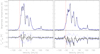 |
Fig. 12 Left panel: HI emission/absorption profile towards the bright southern component of the radio continuum arc-shaped feature. Right panel: same for the extragalactic source at the north of the nebula. The error envelopes are plotted withblue dotted lines. Vertical red lines indicate the velocity of the tangent point. |
6.3 Possible triggered star formation
The spatial distribution of the candidate YSOs along the borders of the IR nebula and the densest part of the molecular gas (see Sect. 5.2) is indicative of a triggered star-forming process such as collect-and-collapse (C&C; Elmegreen & Lada 1977) or radiative driven implosion (RDI; Lefloch & Lazareff 1994) might be acting on the nebula.
In order to test the C&C mechanism, we use the classical model of Whitworth et al. (1994) for expanding HII regions. Then, we estimated the fragmentation time, tfrag, and the radius of the HII region when the fragmentation occurs, Rfrag, as:
 (17)
(17)
 (18)
(18)
with a0.2 as the isothermal sound speed in the compressed layer in units of 0.2 km s−1 (as∕0.2 km s−1), n3 the surrounding homogeneous infinite medium into which the HII region expands, in units of 103 cm−3 (n0 ∕103 cm−3), and N49 the number of ionizing Lyman continuum photons, in units of 1049 s−1 ( /1049 s−1). We adopt as = 0.2 km s−1 for the collected layer (likely a lower limit since both turbulence and extra heating from intense subLyman continuum photons leaking from the HII region could increase this value) and
  = 2.5 × 1047 s−1 (see Sect. 4). To estimate the initial density, n0, we averaged the total mass of the molecular gas around S169 (~(7.4 ± 4.4) × 103 M⊙) over a sphere of 2.3 ± 0.8 pc in radius, which yields a density in the range of n0 = (0.35–12) × 103 cm−3. Thus, we obtain tfrag in the range between 0.5 and 2.2 Myr and Rfrag between 1.1 and 7.4 pc.
A comparison between Rfrag and the present radius of the nebula suggests (within errors) that the C&C process maybe acting in S169. On the contrary, the estimated fragmentation time is higher than the tdyn derived for the region in Sect. 6.1. Thus, there is no conclusive evidence to support that protostellar objects at the borders of S169 could have been formed as a result of the C&C mechanism. We ought to keep in mind, however, that the model of Whitworth et al. (1994) is valid for evolution of the HII regions only in a uniform molecular environment, which is certainly not the case with S169.
Regarding the possibility that the RDI process is taking place in certain regions of the nebula, a more detailed study is required, with better angular resolutions of both the molecular and radio continuum data. Nevertheless, we can clearly conclude that the presence of the intense PDR emission detected as a bright rim of the densest molecular feature suggests that the RDI process could be responsible for the formation of some candidate YSOs. In fact, an alternative scenario for the star formation in S 169 could be that proposed by Walch et al. (2015), which considers the action of massive stars on a fractal molecular cloud resulting in a hybrid mechanism that combines elements of C&C and RDI and which has the capability to generate shell structures with dense clumps within them. If this were the case for S169, the denser region where IRAS 12326-6245 is located could be explained by considering an initial non-uniform molecular cloud with a significant increase in density and, thus, the RDI process could be the main action responsible for the formation of the candidate YSOs located behind this border and, in particular, for the IR source.
7 Summary
As part of a broader project aimed at characterizing and studying the physical properties of Galactic IR bubbles and their surroundings, we present a multiwavelength analysis of the southern IR dust bubble S169 associated with the massive star forming core IRAS 12326-6245. To analyze the characteristics of the molecular gas in the whole nebula, we use CO (2–1), 13 CO (2–1), C18 O (2–1) line data, while for the IRAS source we also use HCN (3–2), and HCO+ (3–2) data, all obtained with the APEX telescope. To study the characteristics of the dust and ionized gas, as well as to investigate the presence of stellar and protostellar objects in the nebula, we use archival data.
The analysis of the CO (2–1), 13CO (2–1), and C18O (2–1) data allows us to identify the molecular gas linked to the nebula. We report three molecular components at approximately −39, −25, and −17 km s−1 (components A, B, and C), which are morphologically correlated with different regions of the IR nebula. The component at −39 km s−1 (component A) is associated with the brightest part of the IR nebula (at the southern region) and is the only one detected in 13 CO (2–1) and C18 O (2–1) emissions. For this component, we have identified six molecular condensations (namely MC1, MC2, MC3, MC4, MC5, and MC6) based on the 13 CO and C18 O emissions. These condensations have masses between ~90 and 5500 M⊙, and H2 column densities between ~6 × 10²¹ and 1 × 1023 cm−2. The densestone (MC3) is the molecular counterpart of IRAS 12326-6245, which demonstrates the physicalassociation between the nebula and the IRAS source. An LTE analysis of the HCO+ (3–2) and HCN (3–2) lines on this source, assuming 50 and 150 K, respectively, indicates column densities of N(HCO+) = (5.2 ± 0.1) × 1013 cm−2 and N(HCN) = (1.9 ± 0.5) × 1014 cm−2. For this condensation, an H2 column density up to ~8 × 1023 cm−2 is obtained from the emissionat 870 μm.
The molecular components at −25 and −17 km s−1 (components B and C) seem to be associated with the faintest and more external regions of the IR nebula. Unlike component A, components B and C are not detected in 13CO and C18O emissions, which indicates that they are composed of low-density gas. This can be confirmed from Herschel images at 70, 160, and 350 μm.
With the purpose of explaining the spatial distribution and velocity of components A, B, and C, we propose a very simple model, which consists of a partially complete semisphere structure expanding at ~12 km s−1. According to the model, component A represents the molecular gas approaching at a velocity of −39 km s−1, while component C (feature 3) the molecular gas receding at a velocity of −17 km s−1. The systemic velocity of the molecular gas associated with the bubble is then −25 km s−1, which is the velocity of component B (features 1 and 2). The distribution in the radio continuum emission at 843 MHz suggests an HII region bounded by ionization to the east, north and south, and by density to the west. This appears to be in line with the model proposed for the molecular gas. The model proposed for the molecular gas brings an additional discussion about the distance of IRAS 12326-6245 (and consequently S169) since the radial velocity adopted in the literature for the IRAS source (approximately −39 km s−1) would not be representative of the velocity of the ISM in its surroundings. Instead, we believe that the systemic velocity of the bubble (–25 km s−1) is more adequate for determining its kinematical distance. Then, using the Galactic rotation model and HI absorption profiles, we determine a kinematical distance of 2.03 kpc for S169 and IRAS 12326-6245.
Using point source catalogs, we identify10 ionizing stars candidates projected onto the cavity. They have spectral types between O9V and B2, which are necessary to sustain the current level of ionization of the HII region. We also identify a number of candidate YSOs projected mostly onto component A, more precisely: MC3, MC4, and MC5, confirming that active star formation has developed along the borders of the bubble. After comparing the fragmentation time and fragmentation radius with the age and current radius of the nebula, we cannot assert that the C&C process is acting in the collected layers of gas at the edge of the bubble. We do keep in mind, however, the limitations of the models applied to S169 and the possibility thatother triggering star-forming processes, such as RDI or a combination of both, RDI and C&C, could be acting in the region.
In summary, the infrared bubble S169 is a relatively young HII region that has profoundly affected its surroundings, creating a molecular shell that continues to possess a large expanding motion and where several condensations host candidate protostellar objects in their dense interiors, with the source IRAS 12326-6245 standing out as the most striking among them.
Acknowledgements
We would like to thank the anonymous referee for his/her helpful comments and suggestions that led to the improvement of this paper. N.U.D and M.A.C acknowledge support from UNLP, PPID G005 and CONICET grant PIP 112−201701−00507 (Argentina).L.B. and R.F. acknowledges support from CONICYT project Basal AFB-170002. E.M. acknowledges support from the Brazilian agency CNPq (grant 150465/2019-0). L.A.S acknowledges support from UNLP PPID G005 grant. S.C., L.A.S. and E.M.R. are partially funded by CONICET grant PIP 112-201701-00604 (Argentina).
Appendix A Identified candidate YSOs
YSO candidates obtained from MSX, WISE, and Spitzer catalogs.
References
- Allen, L. E., Calvet, N., D’Alessio, P., et al. 2004, ApJS, 154, 363 [NASA ADS] [CrossRef] [Google Scholar]
- Alvarez, H., May, J., & Bronfman, L. 1990, ApJ, 348, 495 [NASA ADS] [CrossRef] [Google Scholar]
- Anderson, L. D., Zavagno, A., Deharveng, L., et al. 2012, A&A, 542, A10 [NASA ADS] [CrossRef] [EDP Sciences] [Google Scholar]
- Anderson, L. D., Deharveng, L., Zavagno, A., et al. 2015, ApJ, 800, 101 [NASA ADS] [CrossRef] [Google Scholar]
- Araya, E., Hofner, P., Kurtz, S., Bronfman, L., & DeDeo, S. 2005, ApJS, 157, 279 [NASA ADS] [CrossRef] [Google Scholar]
- Beichman, C. A., Neugebauer, G., Habing, H. J., Clegg, P. E., & Chester, T. J., eds. 1988, Infrared astronomical satellite (IRAS) catalogs and atlases, (Singapore: IRAS) 1 [Google Scholar]
- Benjamin, R. A., Churchwell, E., Babler, B. L., et al. 2003, PASP, 115, 953 [NASA ADS] [CrossRef] [Google Scholar]
- Bloemen, J. B. G. M., Strong, A. W., Mayer-Hasselwander, H. A., et al. 1986, A&A, 154, 25 [NASA ADS] [Google Scholar]
- Bock, D. C. J., Large, M. I., & Sadler, E. M. 1999, AJ, 117, 1578 [NASA ADS] [CrossRef] [Google Scholar]
- Borissova, J., Bonatto, C., Kurtev, R., et al. 2011, A&A, 532, A131 [NASA ADS] [CrossRef] [EDP Sciences] [Google Scholar]
- Bronfman, L., Nyman, L. A., & May, J. 1996, A&AS, 115, 81 [Google Scholar]
- Cappa, C. E., Duronea, N., Firpo, V., et al. 2016, A&A, 585, A30 [NASA ADS] [CrossRef] [EDP Sciences] [Google Scholar]
- Carpenter, J. M., Hillenbrand, L. A., & Skrutskie, M. F. 2001, AJ, 121, 3160 [NASA ADS] [CrossRef] [Google Scholar]
- Caswell, J. L. 1998, MNRAS, 297, 215 [NASA ADS] [CrossRef] [Google Scholar]
- Caswell, J. L. 2009, PASA, 26, 454 [NASA ADS] [CrossRef] [Google Scholar]
- Chaisson, E. J. 1976, in Frontiers of Astrophysics, ed. E. H. Avrett (Berlin: Springer), 259 [Google Scholar]
- Churchwell, E., Povich, M. S., Allen, D., et al. 2006, ApJ, 649, 759 [NASA ADS] [CrossRef] [Google Scholar]
- Churchwell, E., Watson, D. F., Povich, M. S., et al. 2007, ApJ, 670, 428 [NASA ADS] [CrossRef] [Google Scholar]
- Clemens, D. P. 1985, ApJ, 295, 422 [NASA ADS] [CrossRef] [Google Scholar]
- Cohen, R. S., Grabelsky, D. A., May, J., et al. 1985, ApJ, 290, L15 [NASA ADS] [CrossRef] [Google Scholar]
- Comito, C., Schilke, P., Phillips, T. G., et al. 2005, ApJS, 156, 127 [NASA ADS] [CrossRef] [Google Scholar]
- Cousins, A. W. J. 1978, The Observatory, 98, 54 [NASA ADS] [Google Scholar]
- Dedes, C., Leurini, S., Wyrowski, F., et al. 2011, A&A, 526, A59 [NASA ADS] [CrossRef] [EDP Sciences] [Google Scholar]
- Deharveng, L., Lefloch, B., Kurtz, S., et al. 2008, A&A, 482, 585 [NASA ADS] [CrossRef] [EDP Sciences] [Google Scholar]
- Deharveng, L., Zavagno, A., Schuller, F., et al. 2009, A&A, 496, 177 [NASA ADS] [CrossRef] [EDP Sciences] [Google Scholar]
- Devine, K., Mori, J., Watson, C., Trujillo, L., & Hicks, M. 2018, ApJ, 861, 117 [CrossRef] [Google Scholar]
- Digel, S. W., Grenier, I. A., Heithausen, A., Hunter, S. D., & Thaddeus, P. 1996, ApJ, 463, 609 [NASA ADS] [CrossRef] [Google Scholar]
- Ducati, J. R., Bevilacqua, C. M., Rembold, S. r. B., & Ribeiro, D. 2001, ApJ, 558, 309 [NASA ADS] [CrossRef] [Google Scholar]
- Dumke, M., & Mac-Auliffe, F. 2010, SPIE Conf. Ser. 7737, 77371J [Google Scholar]
- Duronea, N. U., Cappa, C. E., Bronfman, L., et al. 2017, A&A, 606, A8 [NASA ADS] [CrossRef] [EDP Sciences] [Google Scholar]
- Duronea, N. U., Vasquez, J., Gómez, L., et al. 2015, A&A, 582, A2 [NASA ADS] [CrossRef] [EDP Sciences] [Google Scholar]
- Egan, M. P., Price, S. D., & Kraemer, K. E. 2003, BAAS, 35, 1301 [NASA ADS] [Google Scholar]
- Elmegreen, B. G., & Lada, C. J. 1977, ApJ, 214, 725 [NASA ADS] [CrossRef] [Google Scholar]
- Faúndez, S., Bronfman, L., Garay, G., et al. 2004, A&A, 426, 97 [NASA ADS] [CrossRef] [EDP Sciences] [Google Scholar]
- Figueira, M., Zavagno, A., Deharveng, L., et al. 2017, A&A, 600, A93 [NASA ADS] [CrossRef] [EDP Sciences] [Google Scholar]
- Foreman-Mackey, D., Hogg, D. W., Lang, D., & Goodman, J. 2013, PASP, 125, 306 [Google Scholar]
- Frerking, M. A., Langer, W. D., & Wilson, R. W. 1982, ApJ, 262, 590 [NASA ADS] [CrossRef] [Google Scholar]
- Gaia Collaboration (Prusti, T., et al.) 2016, A&A, 595, A1 [NASA ADS] [CrossRef] [EDP Sciences] [Google Scholar]
- Gaia Collaboration (Brown, A. G. A., et al.) 2018, A&A, 616, A1 [NASA ADS] [CrossRef] [EDP Sciences] [Google Scholar]
- Güsten, R., Nyman, L. Å., Schilke, P., et al. 2006, A&A, 454, L13 [NASA ADS] [CrossRef] [EDP Sciences] [Google Scholar]
- Gutermuth, R. A., Megeath, S. T., Myers, P. C., et al. 2009, ApJS, 184, 18 [NASA ADS] [CrossRef] [Google Scholar]
- Henden, A. A., Terrell, D., Welch, D., & Smith, T. C. 2010, BAAS, 42, 470.11 [Google Scholar]
- Henning, T., Michel, B., & Stognienko, R. 1995, Planet. Space Sci., 43, 1333 [NASA ADS] [CrossRef] [Google Scholar]
- Henning, T., Lapinov, A., Schreyer, K., Stecklum, B., & Zinchenko, I. 2000, A&A, 364, 613 [NASA ADS] [Google Scholar]
- Hildebrand, R. H. 1983, QJRAS, 24, 267 [NASA ADS] [Google Scholar]
- Hill, T., Burton, M. G., Minier, V., et al. 2005, MNRAS, 363, 405 [NASA ADS] [CrossRef] [Google Scholar]
- Hunter, S. D., Bertsch, D. L., Catelli, J. R., et al. 1997, ApJ, 481, 205 [NASA ADS] [CrossRef] [Google Scholar]
- Inoue, A. K. 2001, AJ, 122, 1788 [NASA ADS] [CrossRef] [Google Scholar]
- Junkes, N., Fuerst, E., & Reich, W. 1992, A&A, 261, 289 [Google Scholar]
- Kendrew, S., Beuther, H., Simpson, R., et al. 2016, ApJ, 825, 142 [NASA ADS] [CrossRef] [Google Scholar]
- Kharchenko, N. V., & Roeser, S. 2009, VizieR Online Data Catalog: I/280B [Google Scholar]
- Koenig, X. P., Leisawitz, D. T., Benford, D. J., et al. 2012, ApJ, 744, 130 [NASA ADS] [CrossRef] [Google Scholar]
- König, C., Urquhart, J. S., Csengeri, T., et al. 2017, A&A, 599, A139 [NASA ADS] [CrossRef] [EDP Sciences] [Google Scholar]
- Koornneef, J. 1983, A&A, 128, 84 [NASA ADS] [Google Scholar]
- Kurtz, S., Cesaroni, R., Churchwell, E., Hofner, P., & Walmsley, C. M. 2000, in Protostars and Planets IV, ed. V. Mannings, A. P. Boss, & S. S. Russell (Tucson: University of Arizona Press), 299 [Google Scholar]
- Langer, W. D., & Penzias, A. A. 1993, ApJ, 408, 539 [NASA ADS] [CrossRef] [Google Scholar]
- Lefloch, B., & Lazareff, B. 1994, A&A, 289, 559 [NASA ADS] [Google Scholar]
- Liu, H.-L., Wu, Y., Li, J., et al. 2015, ApJ, 798, 30 [NASA ADS] [CrossRef] [Google Scholar]
- Lumsden, S. L., Hoare, M. G., Oudmaijer, R. D., & Richards, D. 2002, MNRAS, 336, 621 [NASA ADS] [CrossRef] [Google Scholar]
- MacLeod, G. C., Scalise, E. J., Saedt, S., Galt, J. A., & Gaylard, M. J. 1998, AJ, 116, 1897 [NASA ADS] [CrossRef] [Google Scholar]
- Martins, F., Schaerer, D., & Hillier, D. J. 2005, A&A, 436, 1049 [NASA ADS] [CrossRef] [EDP Sciences] [Google Scholar]
- McClure-Griffiths, N. M., Dickey, J. M., Gaensler, B. M., et al. 2005, ApJS, 158, 178 [NASA ADS] [CrossRef] [Google Scholar]
- Miettinen, O., Harju, J., Haikala, L. K., & Pomrén, C. 2006, A&A, 460, 721 [NASA ADS] [CrossRef] [EDP Sciences] [Google Scholar]
- Molinari, S., Swinyard, B., Bally, J., et al. 2010, A&A, 518, L100 [NASA ADS] [CrossRef] [EDP Sciences] [Google Scholar]
- Möller, T., Endres, C., & Schilke, P. 2017, A&A, 598, A7 [NASA ADS] [CrossRef] [EDP Sciences] [Google Scholar]
- Ossenkopf, V.,& Henning, T. 1994, A&A, 291, 943 [Google Scholar]
- Osterloh, M., Henning, T., & Launhardt, R. 1997, ApJS, 110, 71 [NASA ADS] [CrossRef] [Google Scholar]
- Panagia, N., & Walmsley, C. M. 1978, A&A, 70, 411 [NASA ADS] [Google Scholar]
- Parker, Q. A., Phillipps, S., Pierce, M. J., et al. 2005, MNRAS, 362, 689 [NASA ADS] [CrossRef] [Google Scholar]
- Povich, M. S., Stone, J. M., Churchwell, E., et al. 2007, ApJ, 660, 346 [Google Scholar]
- Preibisch, T., Roccatagliata, V., Gaczkowski, B., & Ratzka, T. 2012, A&A, 541, A132 [NASA ADS] [CrossRef] [EDP Sciences] [Google Scholar]
- Reid, M. J., Menten, K. M., Brunthaler, A., et al. 2014, ApJ, 783, 130 [Google Scholar]
- Reynoso, E. M., Cichowolski, S., & Walsh, A. J. 2017, MNRAS, 464, 3029 [Google Scholar]
- Rieke, G. H., & Lebofsky, M. J. 1985, ApJ, 288, 618 [Google Scholar]
- Rohlfs, K., & Wilson, T. L. 2004, Tools of radio astronomy (Berlin: Springer) [Google Scholar]
- Samal, M. R., Zavagno, A., Deharveng, L., et al. 2014, A&A, 566, A122 [NASA ADS] [CrossRef] [EDP Sciences] [Google Scholar]
- Schmidt-Kaler. Th. 1982, in Landolt-Bornstein New Series, Group VI, eds. K. Schaifers, & H. H. Voigt (Berlin: Springer-Verlag), 2b [Google Scholar]
- Schuller, F., Menten, K. M., Contreras, Y., et al. 2009, A&A, 504, 415 [NASA ADS] [CrossRef] [EDP Sciences] [Google Scholar]
- Skrutskie, M. F., Cutri, R. M., Stiening, R., et al. 2006, AJ, 131, 1163 [NASA ADS] [CrossRef] [Google Scholar]
- Solomon, P. M., Rivolo, A. R., Barrett, J., & Yahil, A. 1987, ApJ, 319, 730 [Google Scholar]
- Strong, A. W., & Mattox, J. R. 1996, A&A, 308, L21 [NASA ADS] [Google Scholar]
- Tenorio-Tagle, G. 1979, A&A, 71, 59 [NASA ADS] [Google Scholar]
- Urquhart, J. S., Busfield, A. L., Hoare, M. G., et al. 2007, A&A, 461, 11 [NASA ADS] [CrossRef] [EDP Sciences] [Google Scholar]
- Vassilev, V., Meledin, D., Lapkin, I., et al. 2008, A&A, 490, 1157 [NASA ADS] [CrossRef] [EDP Sciences] [Google Scholar]
- Walch, S., Whitworth, A. P., Bisbas, T. G., Hubber, D. A., & Wünsch, R. 2015, MNRAS, 452, 2794 [Google Scholar]
- Watson, C., Povich, M. S., Churchwell, E. B., et al. 2008, ApJ, 681, 1341 [Google Scholar]
- Wenger, T. V., Balser, D. S., Anderson, L. D., & Bania, T. M. 2018, ApJ, 856, 52 [Google Scholar]
- Whitworth, A. P., Bhattal, A. S., Chapman, S. J., Disney, M. J., & Turner, J. A. 1994, MNRAS, 268, 291 [NASA ADS] [CrossRef] [Google Scholar]
- Wright, E. L., Eisenhardt, P. R. M., Mainzer, A. K., et al. 2010, AJ, 140, 1868 [Google Scholar]
- Yamaguchi, R., Akira, M., & Yasuo, F. 1999, in Star Formation 1999, ed. T. Nakamoto (Cambridge: Cambridge University Press), 383 [Google Scholar]
- Zavagno, A., Deharveng, L., Comerón, F., et al. 2006, A&A, 446, 171 [NASA ADS] [CrossRef] [EDP Sciences] [Google Scholar]
- Zinchenko, I., Henkel, C., & Mao, R. Q. 2000, A&A, 361, 1079 [NASA ADS] [Google Scholar]
This publication is based on data acquired with the Atacama Pathfinder Experiment (APEX) under program ID C-098.F-9701. APEX is a collaboration between the Max-Planck-Institut fur Radioastronomie, the European Southern Observatory, and the Onsala Space Observatory.
Herschel is an ESA space observatory with science instruments provided by European-led Principal Investigator consortia and with important participation from NASA (http://www.cosmos.esa.int/web/herschel/science-archive).
All Tables
Observed parameters obtained from the emission lines and physical properties derived for the molecular condensations MC1 to MC6.
All Figures
|
Fig. 1 Composite image of S169 and its environs showing the (IRAC-GLIMPSE) emissions at 8.0 (red) and 5.8 μm (green). The superCOSMOS Hα emission is in blue. White contours depict the continuum emission at 870 μm (ATLASGAL) arising from IRAS 12326-6245. |
| In the text | |
|
Fig. 2 Total averaged spectra of CO (2–1) (red), 13CO (2–1) (green), and C18 O (2–1) (blue) obtained within a region of ~14′ × 14′ centered on RA, Dec (J2000) = (12h 35m 44s, −63°00′08′′). |
| In the text | |
|
Fig. 3 Spatial distribution of the C18O(2–1) emission (left panel), 13CO(2–1) emission (middle panel), and CO(2–1) emission (right panel) in the velocity interval from approximately −42 to –37 km s−1 (component A). In the left panel, the contours are 0.35 (~3 rms), 0.7, 1.15, 2, 3, 5, and 7 K km s−1. In the middle panel the contour levels are 0.5 (~6 rms), 1, 1.5, 2, 2.5, 3, 4, 5, 7, 9, 11, 13, and 15 K km s−1. In the right panel the contour levels are 1.5 (~20 rms), 2, 2.5, 3, 4, 5, 6, 8, 10, 14, 18, 22, and 26 K km s−1 (Tmb). Identified molecular condensations are indicated in yellow over the 13CO (2–1) emission. |
| In the text | |
|
Fig. 4 Panel a: emission distribution of the 13CO(2–1) line in the total velocity range from –37 to –42 km s−1 (white contours and blue color scale) superimposed on the IRAC-GLIMPSE images at 8.0 and 5.8 μm (red and green color scales, respectively). The contours levels are the same than those shown in the middle panel of Fig. 3. Panels b to i: channel maps of the 13 CO (2–1) line emission in velocity intervals of 0.7 km s−1 (white contours) in the velocity range from –36.7 to –42.5 km s−1 superimposed on the 8.0 and 5.8 μm (IRAC-GLIMPSE) emissions (red and green color scales) and 870 μm ATLASGAL emission (blue color scale) inside the 3 rms limit. Contours levels are 0.9 (~5.5 rms), 2.6, 4.4, 6.2, 7.9, 10, 12, 16, and 20 K km s−1. The velocityinterval is indicated in the top right corner of each panel. |
| In the text | |
|
Fig. 5 Upper panel: spectral line and LTE model of the HCN (3–2) line obtained from LTE-MCMC calculations assuming Texc = 150 K (see text), with a resulting density of N = (1.9 ± 0.5) × 1014 cm−2. The blue line indicates the residual obtained from the subtraction between the observation and LTE model. In colors: spatial distribution of the HCN (3–2) emission in the velocity interval from −47.6 to −29.2 km s−1 (color blue and white contours) superimposed on the IRAC 8 and 5.8 μm emissions (red and green colors). Lower panel: same as above for the HCO+ (3–2) line, assuming Texc = 50 K, with a resulting density of N = (5.2 ± 0.1) × 1013 cm−2. The HCO+ (3–2) emission distribution is in the velocity interval from −44.8 to −32.5 km s−1. The contour levels for the HCN (3–2) are 0.25 (~5 rms), 0.85, 2.2, and 4.0 K km s−1; and for the HCO+ (3–2) line, they are 0.28(~5 rms), 0.8, 2.4, and 5 K km s−1 |
| In the text | |
|
Fig. 6 Upper panel: spatial distribution of the CO emission (blue color scale and white contours) in the velocity interval from −28.9 km s−1 to −18.9 km s−1 (component B) superimposed on the IRAC 8 μm and 5.8 μm emissions (red and green color scales). The contour levels start from 0.95 K km s−1 (~9 rms) in stepsof 0.5 K km s−1. Lower panel: spatial distribution of the CO emission in the velocity interval from −18.2 to −12.7 km s−1 (component C). The contour levels start from 0.85 K km s−1 (~7 rms) in stepsof 0.4 K km s−1. |
| In the text | |
|
Fig. 7 Upper panel: three-color composite image of S169: Herschel PACS 70 and 160 μm emission are in red and green, respectively. Herschel SPIRE 350 μm emission is in blue. Black contours underline de IRAC-GLIMPSE 8 μm emission at 35, 55, 75, 105, 150, 170, 300, and 500 MJy sr−1. Middle panel: dust temperature map derived from the 70 and 160 μm emission. The color temperature scale is on the right. Lower panel: column density map obtained from the 160 μm emission. Dashed black contours indicate the location of molecular concentrations MC1 to MC6 for orientation. |
| In the text | |
|
Fig. 8 Radio continuum emission distribution at 843 MHz (blue color and white contours), superimposed on the 8 and 5.8 μm emission (red and green color). Contours levels are 3.1 (~3 rms), 4.5, 6.3, 7.6, 12, 20, 30, 40, 100, 200, 300, and 400 mJy beam−1. |
| In the text | |
|
Fig. 9 Color magnitude diagram of stars searched in a region centered in S169. Black dots are young spectral type stars with different reddening values (see text in Sect. 5). Magenta, green, and yellow crosses represent the O9V, B1V, and B2V (or later) stars, all of them ionizing candidate stars displayed with the same colors in Fig. 10. Green and black curves represent the MS shifted according to the distance modulus adopted with and without reddening, respectively. Red line indicates the normal reddening path (Rv = 3.1). |
| In the text | |
|
Fig. 10 MSX, WISE, and Spitzer candidate YSOs projected onto the IRAC-GLIMPSE image at 8.0 and 5.8 μm. Cyan diamonds indicate the MSX sources, blue circles and blue squares indicate WISE Class I and Class II sources, respectively, and green circles and green squares indicate the Spitzer Class I and Class II sources, respectively. The numerical references of YSOs are based on those from Table A.1. The size of the symbols do not necessary match the angular size of the sources. Ionizing candidate stars identified in Sect 5.1 are also indicated by crosses in magenta (O9V), green (B1V), and yellow (B2V or later). White contours indicate the 13 CO emission of component A (first contour level ~8 rms) and theCO emission of feature 1 (first contour level ~13 rms), feature 2 (first contour level ~12 rms), and feature 3 (first contour level ~10 rms). |
| In the text | |
|
Fig. 11 Simple sketch of the proposed model to explain the morphology and velocity of the molecular gas associated with S169. The right ascension axis, as visualized by the observer, is indicated as reference (the declination axis is perpendicular to the planeof the sketch, increasing towards the reader). |
| In the text | |
|
Fig. 12 Left panel: HI emission/absorption profile towards the bright southern component of the radio continuum arc-shaped feature. Right panel: same for the extragalactic source at the north of the nebula. The error envelopes are plotted withblue dotted lines. Vertical red lines indicate the velocity of the tangent point. |
| In the text | |
Current usage metrics show cumulative count of Article Views (full-text article views including HTML views, PDF and ePub downloads, according to the available data) and Abstracts Views on Vision4Press platform.
Data correspond to usage on the plateform after 2015. The current usage metrics is available 48-96 hours after online publication and is updated daily on week days.
Initial download of the metrics may take a while.