| Issue |
A&A
Volume 645, January 2021
|
|
|---|---|---|
| Article Number | A133 | |
| Number of page(s) | 18 | |
| Section | Cosmology (including clusters of galaxies) | |
| DOI | https://doi.org/10.1051/0004-6361/202038207 | |
| Published online | 26 January 2021 | |
Diagnosing the interstellar medium of galaxies with far-infrared emission lines
I. The [C II] 158 μm line at z ∼ 0
1
Kapteyn Astronomical Institute, University of Groningen, Landleven 12, 9747 AD Groningen, The Netherlands
e-mail: This email address is being protected from spambots. You need JavaScript enabled to view it.
2
SRON Netherlands Institute for Space Research, Landleven 12, 9747 AD Groningen, The Netherlands
3
Lorentz Institute for Theoretical Physics, Leiden University, 2333 CA Leiden, The Netherlands
Received:
20
April
2020
Accepted:
24
November
2020
Abstract
Context. Atomic fine structure lines have been detected in the local Universe and at high redshifts over the past decades. The [C II] emission line at 158 μm is an important observable as it provides constraints on the interstellar medium (ISM) cooling processes.
Aims. We develop a physically motivated framework to simulate the production of far-infrared line emission from galaxies in a cosmological context. This first paper sets out our methodology and describes its first application: simulating the [C II] 158 μm line emission in the local Universe.
Methods. We combine the output from EAGLE cosmological hydrodynamical simulations with a multi-phase model of the ISM. Gas particles are divided into three phases: dense molecular gas, neutral atomic gas, and diffuse ionised gas (DIG). We estimate the [C II] line emission from the three phases using a set of CLOUDY cooling tables.
Results. Our results agree with previous findings regarding the contribution of these three ISM phases to the [C II] emission. Our model shows good agreement with the observed L[C II–star formation rate (SFR) relation in the local Universe within 0.4 dex scatter.
Conclusions. The fractional contribution to the [C II] line from different ISM phases depends on the total SFR and metallicity. The neutral gas phase dominates the [C II] emission in galaxies with SFR ∼ 0.01–1 M⊙ yr−1, but the ionised phase dominates at lower SFRs. Galaxies above solar metallicity exhibit lower L[C II/SFR ratios for the neutral phase. In comparison, the L[C II/SFR ratio in the DIG is stable when metallicity varies. We suggest that the reduced size of the neutral clouds, caused by increased SFRs, is the likely cause for the L[C II deficit at high infrared luminosities, although EAGLE simulations do not reach these luminosities at z = 0.
Key words: ISM: lines and bands / Galaxy: formation / Galaxy: evolution / ISM: clouds / evolution / methods: numerical
© ESO 2021
1. Introduction
Over the past decades, significant efforts to develop theoretical models have helped improve our knowledge of how galaxies form and evolve. Implementations of hydrodynamical simulations (e.g.,, Vogelsberger et al. 2014; Hopkins et al. 2014; Schaye et al. 2015; Pillepich et al. 2018) and semi-analytic models (e.g., Somerville & Primack 1999; Cole et al. 2000; Croton et al. 2006) have provided fundamental insights. Most models can now roughly reproduce the observed specific star formation rate (SFR) and mimic the scenario where more massive galaxies formed their stars earlier than lower mass galaxies, an effect known as ‘downsizing’ (Cowie et al. 1996; Pérez-González et al. 2008; Haines et al. 2017). These implementations agree, within a factor of three, with physical properties of galaxies and, in recent years, have begun to converge regarding physical interpretations (Somerville & Davé 2015).
One critical question, tackled by several works in recent years (see e.g., Nagamine et al. 2006; Vallini et al. 2013, 2015; Katz et al. 2017, 2019; Pallottini et al. 2017a,b; Olsen et al. 2015, 2017; Lupi & Bovino 2020; Lupi et al. 2020; Moriwaki et al. 2018; Arata et al. 2020), is how to include the cooling processes of the interstellar medium (ISM) in galactic theoretical models beginning from early epochs. Unfortunately, there is still no single model capable of reproducing all the observational data across all of cosmic history. The balance of gas heating and cooling in the ISM environment (which affects physical properties such as temperature and density) is central to theoretical models. Owing to observational constraints, our ISM knowledge mainly comes from our Galaxy and its nearby cosmic neighbourhood, where cold atomic clouds (cold neutral medium, CNM), diffuse warm neutral and ionised emission (WNM and WIM), and H II regions are distinguishable (e.g., Hollenbach & Tielens 1999; Wolfire et al. 1995, 2003; Kaufman et al. 1999).
Far-infrared (FIR) emission line observations of nearby galaxies that trace these phases of the ISM (Díaz-Santos et al. 2017; Herrera-Camus et al. 2018a) are an important tool for understanding ISM cooling processes and their relation with the SFR, especially in cool gas where permitted lines of hydrogen cannot be excited (< 104 K). However, the current resolution of (most) instruments limits the capability to provide spatially resolved line observations of high-redshift galaxies as in nearby galaxies. There are a few exceptions: Gas an dust clouds can be observed at high redshifts using high spatial resolution with ALMA (e.g., Oteo et al. 2017) or using gravitational lensing (Dessauges-Zavadsky et al. 2019). Extrapolating observations from the local Universe is not a good option as the ISM phases are likely to be different at earlier times. For example, gas-phase metallicities change with redshift, which will have an impact on the ISM phases (Bialy & Sternberg 2019). The growing body of FIR line observations at high-redshift has so far mainly been interpreted based on empirical relations. For example, the L[C II–SFR relations obtained by De Looze et al. (2014) are used to interpret high-redshift galaxies (Inoue et al. 2016; Pentericci et al. 2016; Knudsen et al. 2016). However, over the last few years, new high redshift observations have begun to use emission models to interpret the observations of these lines (e.g., Maiolino et al. 2015; Carniani et al. 2017; Bakx et al. 2020; Bethermin et al. 2020).
Hydrodynamical simulations represent one of the most promising methods to avoid this extrapolation from the local Universe to high redshifts. These simulations can predict the interplay between dark matter and baryons in the large-scale structure and the final properties of galaxies (Dayal & Ferrara 2018). However, this method is computationally expensive if all the relevant physics are considered. Limitations in spatial resolutions and simulation techniques have to be taken into account in the sub-grid physics in different box sizes (see Dayal & Ferrara 2018, their Table 1). Fortunately, zoom-in techniques are starting to bridge the gap between individual stellar and galactic scales, which help to model the general ISM (Somerville & Davé 2015). Therefore, hydrodynamical simulations can help us to predict emission lines at different cosmic epochs and characterise the ISM at different cosmic times (Pallottini et al. 2017a).
The [C II] 158 μm emission line is one of the brightest emission lines in the FIR. Its luminosity is equivalent to values around 1% of the FIR luminosity of galaxies (e.g., Stacey et al. 1991; Brauher et al. 2008). It is an easily observed line that traces various phases of the ISM where gas is exposed to energies above the carbon ionisation potential (11.3 eV compared to 13.6 eV for hydrogen). [C II] can be considered as a robust cooling line (in the range of 20–8000 K) of the ISM, acting as a thermostat (Gong et al. 2012; Goldsmith et al. 2012; Olsen et al. 2015).
Nevertheless, [C II] is difficult to interpret, as it arises from diverse environments: CNM, WNM and WIM. In addition, at higher FIR luminosities, the luminosity of [C II] over the FIR luminosity increases at a lower rate, an effect known as the ‘[C II] deficit’ (e.g., Díaz-Santos et al. 2017, who also observed deficits in other emission lines). These problems do not limit the capacity of [C II] for tracing SFR in local luminous infrared galaxies (e.g., Malhotra et al. 2001; Stacey et al. 2010; Díaz-Santos et al. 2013; Herrera-Camus et al. 2015; Díaz-Santos et al. 2017), but a complete understanding of the origin of the deficit is necessary in order to use this line as a SFR indicator in high-redshift galaxies (De Looze et al. 2011; Gullberg et al. 2015; Spilker et al. 2016). Currently, dependencies on metallicities and radiation fields (radiative feedback) seem to be the most probable regulators of the [C II] line luminosity in theoretical (e.g., Malhotra et al. 2001; Muñoz & Oh 2016; Narayanan & Krumholz 2017; Vallini et al. 2017; Ferrara et al. 2019) and observational (Stacey et al. 2010; Díaz-Santos et al. 2017; Herrera-Camus et al. 2018a) studies.
The goal of this paper is to present a model for the ISM [C II] line emission and show its applications in the local Universe (z = 0). We implement this model of FIR line emission to comprehend the ISM physical conditions in galaxies with line properties. We use z = 0 as a benchmark, as locally we have the best observational constraints that cover a diverse range of galaxies in different environments. Our first target is the [C II] 158 μm line at z = 0, for which we assume contributions from the atomic, molecular, and ionised ISM phases to obtain a model of the [C II] emission in galaxies. We model the emission of [C II] by post-processing hydrodynamical simulations from the Evolution and Assembly of GaLaxies and their Environments (EAGLE) project (Schaye et al. 2015; Crain et al. 2015) with a physically motivated model of the ISM. We use CLOUDY (Ferland et al. 1998, 2013, 2017) cooling tables (Ploeckinger & Schaye 2020) to predict line emission to help us constrain different ISM phases in galactic environments. Throughout this paper, we assume the ΛCDM cosmology from Planck results (Planck Collaboration XVI 2014) (Ω = 0.307, ΩΛ = 0.693, H0 = 67.7 km s−1 Mpc−1 and σ8 = 0.8288).
In this paper, we first give an overview of the methods we use to predict the emission lines (Sect. 2). Then, we verify that our results agree with observations of local galaxies in terms of physical parameters and scaling relations (Sect. 3). After that, we discuss the difference between our findings and other papers. (Sect. 4), and finally, we present our conclusions (Sect. 5).
2. Methodology
In the next sections, we describe the sets of simulations we use (Sect. 2.1), the model to characterise the multi-phase structure of the ISM (Sect. 2.2), and the estimation of line luminosity using CLOUDY cooling tables (Sect. 2.3).
2.1. The EAGLE simulations
EAGLE (Schaye et al. 2015; Crain et al. 2015) consists of several cosmological hydrodynamical simulations, run in an N-body smoothed particle hydrodynamics (SPH) code. Briefly, EAGLE adopts a pressure-entropy parameterisation using the description of Hopkins (2013). The simulations include radiative cooling and photo-electric heating (Wiersma et al. 2009a), star formation (Schaye & Dalla Vecchia 2008), stellar evolution and mass loss (Wiersma et al. 2009b), black hole growth (Springel et al. 2005; Rosas-Guevara et al. 2015), and feedback from star formation and active galactic nuclei (AGN; Dalla Vecchia & Schaye 2012).
This work uses three simulations of different sizes and resolutions from EAGLE: REF-L0025N0376, REF-L0100N1504, and RECAL-L0025N0752. Table 1 presents their main characteristics. We use these simulations to compare the implemented model when using different box-sizes and resolutions. Variations in terms of box-size are analysed when comparing the REF-L0100N1504 and REF-L0025N0376 simulations. Variations in terms of resolution are analysed when comparing the REF-L0025N0376 and RECAL-L0025N0752. EAGLE simulations calibrate the physical parameters of the sub-grid routines to reproduce the observed galaxy stellar mass functions at z ≈ 0 (GSMF; Schaye et al. 2015). The sub-grid parameters of the high-resolution, small-box simulation RECAL-L0025N0752 were re-calibrated to account for the increased resolution (Schaye et al. 2015; Crain et al. 2015). REF-L0100N1504 and RECAL-L0025N0752 are similar in terms of ‘weak convergence’, which means numerical results converge in different simulations after re-calibrating the sub-grid parameters (Furlong et al. 2015; Schaye et al. 2015).
EAGLE simulations used in this work.
We selected our sample of galaxies from the EAGLE database (McAlpine et al. 2016) similarly to the study of Thob et al. (2019). We focussed on ‘central’ galaxies, sub-halos containing the particle with the lowest value of the gravitational potential, instead of ‘satellite’ galaxies, to avoid environmental influence on the morphology and kinematics of the galaxies. We used galaxies with at least 300 star particles within 30 pkpc (proper kpc) from the centre of the potential. For REF-L0100N1504, the top 5000 most-gas-massive galaxies are selected to cover the range of gas mass that REF-L0025N0376 cannot cover. Simulated galaxies are retrieved from the SPH data (The EAGLE team 2017) by using FOF (Friends-of-Friends) and SUBFIND algorithms (Springel et al. 2001; Dolag et al. 2009) in the dark matter halos. In the last column of Table 1, we present the total number of galaxies used to calculate line luminosities with our model in each of the simulations.
2.2. The multi-phase ISM model
In this section, we describe the model for the multi-phase ISM using gas and star SPH particles in terms of the simulation properties (Sect. 2.2.1) and three different ISM environments: dense molecular clouds (Sect. 2.2.2), neutral atomic gas (Sect. 2.2.2), and diffuse ionised gas (DIG, Sect. 2.2.3).
2.2.1. Gas and star particle properties
We selected SPH particles inside a volume of radius 30 pkpc to ensure that the derived parameters in our modelling are similar to those in the EAGLE database1 for each galaxy. In Table 2, we present the symbol and the properties from the particle data that we use for the modelling. In addition, we obtained the IDs for the particles and their position to study their spatial distribution.
Physical properties used from the EAGLE data for stars and gas particles.
We retrieved physical parameters from the gas in each of the SPH particles before dividing these SPH into neutral and ionised gas phases. We calculated the total hydrogen number density as
 (1)
(1)
with mH the hydrogen mass, ρ the density and XH the SPH weighted hydrogen abundance. EAGLE imposes a pressure floor expressed as a polytropic equation-of-state as P ≥ Plim(ρ/ρlim)γlim, where γlim = 4/3, Plim, and ρlim are constants (∼ 1.2 × 10⁻¹³ Ba and ∼ 2.23 × 10⁻²⁵g cm−3, Schaye & Dalla Vecchia 2008; The EAGLE team 2017). A temperature threshold is then obtained from Plim = ρlimTlim/(μmH), where μ ≈ 1.23 is the mean molecular weight of the neutral gas. For gas particles limited by the pressure floor, the temperature Tlim is an effective temperature, including unresolved processes in addition to the thermal temperature. We therefore constrain TSPH at n(H) > 0.1 cm−3 to 8000 K, which is typical of the warm ISM (WNM and WIM).
We followed Rahmati et al. (2013) to calculate the fraction of neutral hydrogen η = n(H I)/n(H) given by the ionisation equilibrium n(H I)ΓTot = αAnen(H II) as
 (2)
(2)
where αA is the Case A recombination rate, ΓTot is the total ionisation rate, and ne, n(H I), and n(H II) are the number densities of electrons, neutral hydrogen and ionised hydrogen, respectively. To solve this equilibrium, we used αA from Hui & Gnedin (1997),
![Mathematical equation: $$ \begin{aligned} \displaystyle \alpha _{\rm A} = 1.269 \times 10^{-13} \frac{\lambda ^{1.503}}{\left[ 1 + \left( \frac{\lambda }{0.522} \right)^{0.47}\right]^{1.923}} \mathrm{cm} ^{3}\, \mathrm{s} ^{-1}, \end{aligned} $$](/articles/aa/full_html/2021/01/aa38207-20/aa38207-20-eq3.gif) (3)
(3)
where λ = 2TTR/T, with TTR = 157 807 K, is the ionisation threshold for H I, and T is the gas temperature. ΓTot can be defined as
 (4)
(4)
where ΓPhot is the photo-ionisation rate, and ΓCol is the collisional ionisation rate. ΓCol was calculated following Theuns et al. (1998) as
 (5)
(5)
where
 (6)
(6)
Rearranging Eq. (2) with Eqs. (3)–(6) as
 (7)
(7)
we obtained the neutral fraction η for a given density n(H), temperature T and photo-ionisation rate. With η, we calculated the total neutral mass associated with the neutral phase as mneutral = η × mSPH and at the same time we defined the total ionised gas mass as mionised = mSPH − mneutral.
We took the background interstellar radiation field (ISRF) over the SPH particle due to star formation into account as another important parameter. For this, we assumed that gas in the disk is self-gravitating and obeys the Kennicutt-Schmidt (KS) star-formation law (Schaye & Dalla Vecchia 2008). We calculated the Jeans length as
 (8)
(8)
 (9)
(9)
where cs is the effective sound speed (Schaye & Dalla Vecchia 2008; Schaye 2001), and γ = 5/3 is the adiabatic index (different from the polytropic index γlim). The total pressure for the SPH particle (entropy-weighted, The EAGLE team 2017) is defined as
 (10)
(10)
where E is the entropy. Then the SFR density is
 (11)
(11)
where the KS law exponent is n = 1.4, G is the gravitational constant, the gas fraction fg is assumed to be unity and the absolute star-formation efficiency is A = 1.515 × 10⁻⁴ M⊙ yr−1 kpc−2 (Schaye & Dalla Vecchia 2008; The EAGLE team 2017). The SFR surface density is defined from Eqs. (8) and (11) as ΣSFR = ρSFRLJ. Following Lagos et al. (2015), we determined the background ISRF in units of the Habing radiation field (G0 = 1.6 × 10⁻³ erg cm−2 s−1Habing 1968) as
 (12)
(12)
where ΣSFR, MW = 0.001 M⊙ yr−1 kpc−2 is the value of the SFR surface density in the solar neighbourhood (Bonatto & Bica 2011).
We calculated the ISRF coming directly from the local stars close to the gas particles (inside the smoothing length h of the gas particle) following the procedure described by Olsen et al. (2017). We used the information from starburst99 (Leitherer et al. 2014) stellar models with a mass of 104 M⊙ to obtain a grid of models at different metallicities2 and ages3 for the star particles. A Kroupa initial mass function (IMF) was adopted from starburst99 although the EAGLE simulations used a different IMF (Chabrier); the expected differences in the FUV luminosities (LFUV) are negligible (< 2%) in these range of parameters (Olsen et al. 2017). From these stellar models, we obtained the respective LFUV (calculated as the average luminosity between 912 and 2066 Å, 6 − 13.6 eV) for each metallicity and age. Then we interpolated these values to estimate the LFUV for each of the star particles in the galaxy.
The local radiation field is then defined as
 (13)
(13)
where |rgas − r*, i| is the distance between the gas and star particles, m*, i is the stellar mass and LFUV, i the value of the FUV luminosity for each star particle. We then defined the total ISRF hitting the outer part of the neutral cloud as
 (14)
(14)
where we have normalised the value of  by G0, MW (i.e.
  ), using G0, MW = 9.6 × 10⁻⁴ erg cm−2 s−1 (Seon et al. 2011). Typical values for G0, cloud are in the range ∼0.1–108. The low ranges (∼0.1) are regions where the gas particles are only affected by G0, bkg, while at high ranges (∼108) G0, loc is dominant as the stars particles are very close to the gas particles.
2.2.2. Neutral clouds
Following the work of Olsen et al. (2015), we identified two phases in the environments of the neutral gas clouds that we analyse in this work, the dense molecular gas and the neutral atomic gas. To determine the properties of these phases, the neutral mass mneutral is divided into the neutral clouds by sampling the mass function as observed in the Galactic disk and Local Group:
 (15)
(15)
with β = 1.8 (Blitz et al. 2007). We applied a lower cut on the mass of 104 M⊙ and an upper cut of 106 M⊙ (Narayanan et al. 2008a,b). The remaining gas below the lower limit of 104 M⊙ is discarded and so it goes to the ionised mass (mionised); in general this is below 1% of the mass. The neutral clouds were randomly distributed within 0.5h, with the radial displacement scaling inversely with mcloud, to conserve the mass distribution in the galaxy. Changing this radial distribution limit (0.5h) affects the final luminosities minimally.
We used the entropy to obtain the external pressure (Eq. (10)) and to calculate the radius of the neutral cloud (Rcloud). We took the relative contributions by the cosmic-ray (CR) and magnetic pressure into account, where α0 = 0.4 and β0 = 0.25 following Elmegreen (1989):
 (16)
(16)
Rcloud is then obtained following the virial theorem from a pressure normalised mass-size relation as (Field et al. 2011; Hughes et al. 2013; Faesi et al. 2018)
 (17)
(17)
resulting in sizes of Rcloud ≈ 1–300 pc (Sect. 2.4). For the density inside the neutral cloud, we used a gas distribution described by a Plummer profile:
 (18)
(18)
with Rp = 0.1 Rcloud. Adopting this density profile ensures a finite central density. In addition, Popping et al. (2019) showed that this profile is better at reproducing the [C II] luminosity in galaxies from z = 0 to z = 6 compared to other distributions (power law, logotropic and constant density profiles). With these values, we described the structure for the neutral clouds. In addition, the neutral clouds inherit some physical parameters (e.g., Z,  , XC among others) from the SPH particle.
The [C II] emission arises from within the neutral clouds except from the inner core region, which is shielded from FUV radiation. We calculated the radius where the abundances of C and C+ are equal (RCI) and assumed that all the atoms inside this radius are neutral, so the emission of [C II] in that region is zero. We followed the steps described in Olsen et al. (2015), who used the approach of Röllig et al. (2006) with the following reactions for the formation and destruction of C+:
 (19)
(19)
 (20)
(20)
 (21)
(21)
We solved RCI with the equation
![Mathematical equation: $$ \begin{aligned} 5.13 \times 10^{-10}\, s^{-1} \chi G_{\mathrm{0,cloud} } = n(\mathrm{H} )(R_{\mathrm{CI} }) \left[ a_C X_C + 0.5 k_C \right] \end{aligned} $$](/articles/aa/full_html/2021/01/aa38207-20/aa38207-20-eq25.gif) (22)
(22)
with
 (23)
(23)
where the left-hand side of Eq. (22) is C+ formation (Eq. (19)) and the right-hand side is C+ destruction (Eqs. (20) and (21)). We used the same constants as Olsen et al. (2015) for the recombination and radiative association rate coefficients: aC = 3 × 10⁻¹¹ cm3 s−1 and kC = 8 × 10⁻¹⁶ cm3 s−1 (Pelupessy & Papadopoulos 2009). The normalisation constant (5.13 × 10⁻¹⁰ s−1) comes from the ionisation rate in the photo-dissociation region (PDR) model by Röllig et al. (2006). In the integral, the isotropic radiation field is accounted by μ = 1/cos θ, where θ is the angle between the Poynting vector and the normal direction. The visual extinction correspondingly is defined as AV(RCI) = 0.724σdustZ′⟨n(H)⟩Rcloud ln(Rcloud/RCI) (Pelupessy & Papadopoulos 2009), where σdust = 4.9 × 10⁻²² cm2 is the FUV dust absorption cross section (Mezger et al. 1982), Z′ is the mean metallicity of the galaxy and ⟨n(H)⟩ is the average density inside the neutral cloud. The difference in the opacity between visual and FUV light is set to ξFUV = 3.02 (Röllig et al. 2006). The carbon abundance relative to hydrogen XC comes from the carbon mass fraction of the parent SPH particle. For simplicity, Röllig et al. (2006) assumed that the density of electrons is similar to that of carbon to obtain Eq. (22).
As these calculations are computationally expensive, we created a grid of four variables to solve for RCI, using the following ranges: 4 ≤ log(mcloud[M⊙]) ≤ 6, 18.5 ≤ log(Rcloud[cm]) ≤ 21, −1.5 ≤ log(G0, cloud) ≤ 8 and −7 ≤ log(XC) ≤ − 1.5, all in steps of 0.125 dex. With this grid of ∼1.2 million points, we obtained a solution for RCI for each neutral cloud.
To differentiate neutral atomic gas and dense molecular gas, we needed to define a radius at which molecular hydrogen dominates. We calculated the molecular H2 fraction following Gnedin & Kravtsov (2011) as
 (24)
(24)
where
 (25)
(25)
![Mathematical equation: $$ \begin{aligned} &\Lambda = \ln { \left[ 1 + g D_{\mathrm{MW} }^{3/7} \left( U_{\mathrm{MW} }/15 \right)^{4/7} \right]}, \end{aligned} $$](/articles/aa/full_html/2021/01/aa38207-20/aa38207-20-eq29.gif) (26)
(26)
 (27)
(27)
 (28)
(28)
 (29)
(29)
![Mathematical equation: $$ \begin{aligned} D_* = 1.5 \times 10^{-3} \ln { \left[ 1 + \left( 3 U_{\mathrm{MW} } \right)^{1.7} \right] }, \end{aligned} $$](/articles/aa/full_html/2021/01/aa38207-20/aa38207-20-eq33.gif) (30)
(30)
the metallicity of gas in solar units is DMW = Zgas/Z⊙, and the local UV background is UMW = SFR/SFRMW. Then the molecular fraction can be used for determining the radius at which the transition from atomic to molecular H occurs (RH2) in a Plummer profile (Eq. (18)):
 (31)
(31)
This information helped us to calculate the density and temperature at RH2 in the dense molecular gas and neutral atomic gas regions.
2.2.3. Diffuse ionised gas
For the diffuse ionised gas (DIG), we followed a slightly different approach than that used by Olsen et al. (2015, 2017), where they assumed a DIG cloud with a radius equal to the smoothing length (h). We wanted to avoid dependency on the simulation’s resolution and overproduction of DIG in SPH particles with very large h (≳5 kpc in 100 Mpc boxes, Sect. 2.4). We instead calibrated our models with the estimated luminosity of [N II] lines at 122 and 205 μm emitted almost entirely from the ionised medium. By comparing these lines it is possible to deduce the fractions of the ionised gas (Croxall et al. 2017). For example [N II] at 122 μm is associated with the DIG rather than with a compact H II region (Cormier et al. 2012).
To calibrate the DIG fraction in the [C II] line, we created a distribution of radii of the DIG (RDIG) assuming an isothermal sphere with uniform density. We assumed that the distribution function behaves as a smoothed broken power law for RDIG:
![Mathematical equation: $$ \begin{aligned} p(R_{\mathrm{DIG} })= \left( \frac{R_{\mathrm{DIG} }}{R_{\rm b}} \right)^{-\alpha _1} \left\{ \frac{1}{2} \left[ 1+ \left( \frac{R_{\mathrm{DIG} }}{R_{\rm b}} \right)^{1/\Delta } \right] \right\} ^{( \alpha _1 - \alpha _2 ) \Delta }, \end{aligned} $$](/articles/aa/full_html/2021/01/aa38207-20/aa38207-20-eq35.gif) (32)
(32)
where Rb is the break radius, α1 is the power law index for RDIG ≪ Rb, α2 is the power law index for RDIG ≫ Rb and Δ is the smoothness parameter. We created a grid of different values as described in Table 3 for the parameters in Eq. (32). We fixed the Δ parameter to 0.1 to achieve a distribution with a smooth peak. We estimated the line luminosity for the given grid of values in a random sample (20%) of galaxies from REF-L0100N1504. We only used REF-L0100N1504 for the DIG calibration as the small simulation boxes do not contain enough galaxies to compare with the observational sample.
We used observational data from Fernández-Ontiveros et al. (2016) to calibrate the contribution of the DIG. We used the L[N II]122–SFR, L[N II]205–SFR and L[N II]122/L[N II]205–SFR relations to compare the observational and simulated samples. We considered only cases with a SFR inside the values that the selected simulation could achieve (−2.8 < log(SFR) < 1.7), for a total of 69 observed galaxies. The two datasets (observational and simulated) were binned by SFR into identical bins. We calculated the mean and standard deviation in each bin to compare them using a chi-square (χ2) test. We noticed that χ2 values were not significantly affected by the α parameters, so we selected α1 = −2.0 and α2 = 1.0, assuming that the DIG size is larger than the neutral clouds. We found that the Rb value that minimises the χ2 is Rb ≈ 900 pc.
In Fig. 1 we present the L[N II]–SFR relations at z = 0 from the simulations used in this work compared with the sample of galaxies with [N II] used in the DIG calibration from Fernández-Ontiveros et al. (2016). We recover the same trend of the observed [N II] line luminosities with REF-L0100N1504. The DIG calibration shows a good agreement for simulations with the same resolutions (REF-L0100N1504 and REF-L0025N0376) but RECAL-L0025N0752 is off by less than 1 dex, which is related to the re-calibration (see discussion in Sect. 4.4).
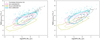 |
Fig. 1. L[N II]122–SFR (left) and L[N II]205–SFR (right) relations for the three simulations used (REF-L0025N0376, RECAL-L0025N0752, and REF-L0100N1504) and the observational sample used for the DIG calibration from Fernández-Ontiveros et al. (2016) (grey dots). The smoothed contours show where 90% (solid) and 50% (dashed) of the galaxies from the respective simulations lie. The remaining 10% of galaxies are represented as dots using the same colours. |
We randomly sampled the DIG radii using Eq. (32) for each galaxy. We used the assigned DIG radii and the ionised mass (mionised) to calculate the density of this ISM phase for each SPH particle. These lead us to densities ranging from around 10−6 to 3 cm−3 for the DIG (due to the limits in CLOUDY cooling tables, Table 4), with a peak at 10−2 cm−3 (see results in Sect. 2.4).
Sampling of gas properties in the CLOUDY grid used in this work.
2.3. Line luminosity prediction
We predicted line luminosities with the help of CLOUDY v17.01 (Ferland et al. 2017), using a set of cooling tables presented by Ploeckinger & Schaye (2020). CLOUDY is a 1D spectral synthesis code that predicts atomic and molecular line intensities in different environments using an escape probability formalism. Here we describe briefly the important aspects of the cooling tables used.
An equally spaced grid was used in the dimensions redshift z, gas temperature log T, metallicity log Z, and gas density log n(H), as presented in Table 4. In this work, we only made use of the redshift bin at z = 0. The importance of using the redshift as a parameter resides on the non-negligible effect on the line emissivity from the cosmic microwave background (CMB). The spin temperature of the [C II] emission is similar to the CMB temperature at high redshift in low density environments (WNM), affecting the [C II] emission. In contrast, at high densities (CNM) the spin temperatures are larger, so the [C II] emission is not affected (Vallini et al. 2015; Pallottini et al. 2017a; Lagache et al. 2018; Olsen et al. 2018a). However, for this study at z = 0, the CMB is not important.
CLOUDY is used to propagate the incident radiation in a plane-parallel gas until the column density Nsh is reached. For gas with temperatures of T ≤ 103 K the shielding column Nsh is assumed to be equal to one half of the Jeans column density
![Mathematical equation: $$ \begin{aligned} \log N_{\rm J} [\mathrm{cm} ^{-2}] = 19.44 + 0.5 \times \left( \log n(\mathrm{H} ) [\mathrm{cm} ^{-3}] + \log T [\mathrm{K} ] \right) \end{aligned} $$](/articles/aa/full_html/2021/01/aa38207-20/aa38207-20-eq36.gif) (33)
(33)
to model the shielding from the edge to the centre of a self-gravitating gas cloud with an extent equal to the Jeans length λJ. For higher temperatures, the column density of the self-shielding gas asymptotically approaches that of the optically thin gas and a maximum column density of Nmax = 1024 cm−2 and a maximum length scale of lmax = 100 kpc are imposed.
For the radiation field, redshift-dependent contributions from the CMB and UV background (Faucher-Giguère 2020) are applied. In addition, the ISRF (‘table ism’ in CLOUDY) and cosmic rays (CR), scaled to solar neighbourhood values, are added depending on the column density. Solar abundances are assumed, with the abundance ratios modified by dust depletion following Jenkins (2009). Primordial abundances are also calculated (when log Z/Z⊙ = −50) using Planck Collaboration XIII (2016) primordial values for helium (not used in this work).
The ‘Orion’ grain distribution (from CLOUDY) is used to take into account other physical effects from dust (e.g., photoelectric heating and charge and collisional processes) by assuming a dust-to-gas ratio dependent on the metallicity and column density (assuming log NH[cm−2] = 20.56 from the gas surface density in the solar neighbourhood, Lagos et al. 2015). Furthermore, polycyclic aromatic hydrocarbons (PAHs) are included but quantum heating is disabled (no ‘qheat’). The large (i.e. more detailed) H2 model in Cloudy is used and the CR photo-dissociation rate is re-scaled to match the UMIST database4 values (see also Shaw et al. 2020).
The two cooling tables we used in this work, ideal for cosmological simulations, have the ISRF and CR rate values reduced by 1 dex relative to the MW values (Black 1987; Indriolo et al. 2007) to better match the observations of the transition between atomic and molecular hydrogen (Ploeckinger & Schaye 2020). In other words, physical parameters decrease: the SFR surface density ΣSFR decreases from 10−3 M⊙ yr−1 kpc−2 to 10−4 M⊙ yr−1 kpc−2, and the CR hydrogen ionisation rate log ζ decreases from −15.7 s−1 to −16.7 s−1. The first table includes self-shielding and the second table is the optically thin counterpart (1-zone unattenuated cloud) of the first table5. The latter provides us with the emissivities of the DIG, approximating this phase as optically thin. We sample and limit the grids to the values presented in Table 4.
We used thermal equilibrium temperatures, where cooling is equal to heating, which depend mainly on two variables n(H) and Z. The temperatures of the gas phases were then obtained with a linear interpolation of the grid with density and metallicity (as other parameters like ISRF or CR depend on these) for the neutral atomic gas, dense molecular gas and DIG phases. This assumption is probably incorrect for the DIG, as ionised regions could be outside thermal equilibrium, because DIG gas can have higher temperatures, but temperature values ≈104 K are commonly assumed when modelling ionised regions (e.g., Haffner et al. 2009; Vandenbroucke & Wood 2019; Ferrara et al. 2019; Ploeckinger & Schaye 2020). For atomic and molecular gas, thermal equilibrium is commonly used in PDR models (Tielens & Hollenbach 1985; Hollenbach & Tielens 1999).
The [C II] line luminosity is then computed from the integral of the [C II] emissivity, Λ[C#x202F;II], interpolated from the CLOUDY cooling table as described above, through the equation
![Mathematical equation: $$ \begin{aligned} L_{\mathrm{[} {\text{ C}}{\small { {\text{II}}}}]} = \int \Lambda _{\rm [{\text{C}}{\small {{\text{II}}}}] } dV = 4 \pi \int _{R_1}^{R_2} \Lambda _{\rm [{\text{C}}{\small {{\text{II}}}}] } R^2 \mathrm{d}R. \end{aligned} $$](/articles/aa/full_html/2021/01/aa38207-20/aa38207-20-eq37.gif) (34)
(34)
The limits of the integral are defined by the three components of the ISM model, DIG, atomic gas and molecular gas; therefore, R1 = 0 and R2 = RDIG for the DIG, R1 = RH2 and R2 = Rcloud for the atomic gas and R1 = RCI and R2 = RH2 for the molecular gas. Ten shells are used to estimate the luminosities for the atomic gas and molecular gas where we assumed that the density follows a Plummer profile (Eq. (18)). In the case of the DIG, one shell is used because we assume a homogeneous density distribution.
2.4. Summary and verification
To summarise, we illustrate the path from the EAGLE simulations (Sect. 2.1) to the total luminosity of [C II] (Sect. 2.3) in Fig. 2. First, we selected a sample of galaxies from the EAGLE database and retrieved the gas and star particle data of the sample. Second, we calculated physical properties such as density and neutral fraction for the gas particles. Local ISRF was calculated with starburst99 models derived from star particles, while background ISFR came from the SFR surface density. The neutral gas mass and the ISRF were used to create the neutral cloud structures inside galaxies, while the ionised gas mass is used to create the DIG. After calibration with the [N II] lines for the DIG, we obtained the luminosity of [C II] line for each phase using CLOUDY cooling tables (Ploeckinger & Schaye 2020). Finally, we calculated the total [C II] luminosity in a galaxy with the contributions from the three ISM phases combined.
 |
Fig. 2. Flowchart of the sub-grid procedures applied to the SPH simulation to simulate line emission in post-processing. For each EAGLE simulation, we obtain the galaxy information from the database and we use the star and gas particle data to implement the ISM model. Next, we calculate physical properties in each phase to obtain the neutral clouds and DIG structures. We use CLOUDY cooling tables (Ploeckinger & Schaye 2020) to get the line luminosity for [C II]. We first calculate L[C II],DIG and then calibrate the ionised gas using the predicted luminosities of the [N II] lines. We then obtain the total line luminosity from the luminosities of the different ISM phases. The dashed lines connect the gas environment to the ingredients of the model. |
We plot the distribution of the sizes for the neutral clouds and DIG (described in Sect. 2.2) in Fig. 3. The values for RH2 show that the molecular regions are in general smaller than RCI. As the neutral clouds are modelled with a Plummer profile (Eq. (31)), the molecular fraction will be restricted to the centre of the neutral clouds at around one pc, so the emission coming from these regions will be less than the atomic gas emission in most cases. In cases where RH2 is very small (fH2 near zero and RCI > RH2), the atomic phase will dominate between Rcloud and RCI. For the case when the shielding is efficient (fH2 ≫ 0), the atomic gas goes from Rcloud to RH2 and the molecular goes from RH2 to RCI. Therefore, RCI is the dominant internal bound for the atomic region in most cases. We sketch these radii in the different neutral clouds in Fig. 2.
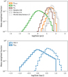 |
Fig. 3. Mean mass-weighted distribution of the sizes of the ISM phases for RECAL-L0025N0752. Upper panel: radii defining the limits of the phases inside the neutral clouds: Rcloud, RH2 and RCI. We compare with sizes of MW clouds (solid and dashed grey lines, Murray 2011; Miville-Deschênes et al. 2017) and local Universe clouds (Bolatto et al. 2008, dotted grey lines). Lower Panel: assumed mean mass-weighted distribution of the radii of the DIG using the smoothing length h (dashed) or Eq. (32) (solid) to define RDIG. |
Typical sizes for these neutral clouds (∼0.5 − 200 pc) agree with observed values in the MW (e.g., Murray 2011; Miville-Deschênes et al. 2017) and in the local Universe (e.g., Bolatto et al. 2008), as presented in the upper panel of Fig. 3. In the case of the DIG, we compared two different cases, using the smoothing length h or Eq. (32). When using h, the DIG sizes can go up to ∼20 kpc, which is the size of some galaxies in the simulations, while with RDIG from Eq. (32), sizes are between 100 pc and 10 kpc with a peak at around 0.9 kpc. Again, in Fig. 2 we sketch, as an example, the DIG as a volumetric region around the neutral clouds.
In Fig. 4 we show the densities and temperatures obtained with the gas particles for the different ISM phases, as well as the initial SPH gas and density from the simulation. Most of the initial gas density fills the area above 104 K and below ∼0.1 cm−3, while the remaining initial gas is distributed along the equation-of-state threshold imposed by EAGLE. The initial gas distribution in the temperature-density plane shows how important it is to implement a physically motivated model for the different ISM phases where EAGLE is incapable of reaching. With our model, the DIG density runs from the lowest density (10−6) to ∼3 cm−3 with a peak around 0.01 cm−3, the atomic density runs from 10−1 to 103.5 cm3 with a peak at 1 cm−3, and the molecular gas density runs from 10 cm−3 to 106 cm−3 with a peak at 105 cm−3. For the temperatures, the DIG range is between 103.2 K and 104.9 K, with a peak around 104 K, in the atomic the temperatures vary from 101 K and 104 K with two peaks around 60 K and 5000 K, and the molecular gas temperature is constrained to a small region between 10 to 300 K due to the H2 heating processes.
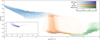 |
Fig. 4. Temperature vs density for the three ISM phases in the RECAL-L0025N0752 galaxies. Each phase is represented with a normalised relative frequency between 0.1% and 100%. We observe that each phase is located in a specific region of the temperature vs density plane. The DIG (blue) is characterised by high temperatures (log T[K]≳3.5) and low densities (log n(H)[cm−3]≲ − 1), atomic gas (orange) by intermediate densities (−1 ≲ log n(H)[cm−3]≲3) with a bridge between high temperatures (log T[K]≈3.5) and low temperatures (log T[K]≈1.4) and molecular gas (green) by high densities (log n(H)[cm−3]≳3) and a range of very low temperatures (log T[K]≈1.1) to intermediate temperatures (log T[K]≈2.5) due to H2 heating processes (Bialy & Sternberg 2019). The temperature-density relation of the original SPH gas particles (inset plot) is shown in purple to demonstrate the need to use a more detailed ISM model when predicting FIR line strengths from these simulations. |
Comparing Fig. 4 with recent simulations of individual local-like galaxies (MW and M51) from Tress et al. (2020a,b), we find similar locations for the atomic gas phases and thermal stable regimes (T ∼ 100 K and T ∼ 104 K). Molecular regions are located in the same regime (T ∼ 20 K and n(H) > 102 cm−3) as well as diffuse ionised gas (T ∼ 104 K and n(H) < 1 cm−3). The only difference is on the step transition we have between the thermal stable regimes. With our CLOUDY grids, the temperatures change from 104 K to 100 K over less than one order of magnitude in density, while Tress et al. (2020a,b) results show a smooth transition that covers two orders of magnitude in density. This transition depends on the assumed metallicity and radiation field (Bialy & Sternberg 2019). Therefore, the difference between our results and Tress et al. (2020a,b) may be related to different implementations in terms of numerical methods and chemical evolution, affecting the ISRF and metallicity.
3. Results
3.1. Contributions of ISM phases to [C II] emission
Various studies report that the atomic phase dominates the fractional contribution of L[C II] in the MW and the local Universe (Pineda et al. 2014; Cormier et al. 2019; Abdullah & Tielens 2020). For example, Cormier et al. (2019) calculate the physical parameters of the Herschel Dwarf Galaxy Survey (HDGS) sample with a mix of two models, for low and high ionisations. They assume that only the dense H II model (high ionisation) produces an atomic gas phase. In terms of their atomic gas fraction there is an average increase in their sample from ∼0.2 to ∼0.5 when log(SFR) [M⊙ yr−1] changes from ∼ − 3 to ∼0. Pineda et al. (2014) calculated the ISM contributions in the MW galactic plane where molecular, atomic, and ionised gas, contribute to 25%, 55%, and 20% of the [C II] luminosity, respectively. However, the contribution of the DIG phase is difficult to estimate accurately. For example, the DIG phase can be more vertically extended in disk galaxies such as the MW, which can cause a difference in the estimated DIG contribution from 4% to 20% as noted by Pineda et al. (2013, 2014). Finally, Abdullah & Tielens (2020) studied the Orion-Eridanus super-bubble and found that the surfaces of molecular clouds, mostly atomic gas, are the main contributors (80%) to the [C II] emission.
We separate the contributions from different ISM phases to L[C II as a function of SFR. We present the median fractional contribution (the luminosity contribution of a given phase to the total luminosity of the galaxy) of these ISM phases in Fig. 5 for the three simulations we have used. These results show the fractional contribution of each of the ISM phases presented in Fig. 5 varies with the simulation used and the total SFR of the galaxy.
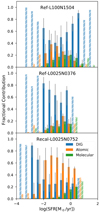 |
Fig. 5. Fractional contributions of the ISM phases to the total L[C II for REF-L0100N1504 (top panel), REF-L0025N0376 (middle panel), and RECAL-L0025N0752 (bottom panel) simulations. Shaded, white-diagonal-striped bars indicate bins with fewer than ten galaxies. The grey lines show the range between the 25th and 75th percentiles. Colours are the same as in Fig. 4. |
We see a general agreement in terms of qualitative trends among the three simulations in Fig. 5. In all simulations, the fractional contributions from the neutral phases increase with increasing SFR, especially for the molecular phase. On the other hand, the DIG fractional contribution decreases with increasing SFR and then flattens, or increases again for REF-L0100N1504. However, the three simulations also exhibit some differences in quantitative terms. The relatively small differences between the two intermediate simulations, REF-L0025N0376 and REF-L0100N1504, are due to sampling noise as the two simulations only differ in size. In particular, the larger box simulation provides a better sampling of the brighter and rarer galaxy population with higher SFRs. The differences between the intermediate and high-resolution simulations are much larger and are due to the GSMF re-calibration, which changes the feedback parameters in the simulation (Schaye et al. 2015). This re-calibration leads to different intrinsic characteristics for the galaxies between the simulations: The stellar feedback produces more outflows of metal-enriched material in RECAL-L0025N0752 (compared to REF-L0100N1504 and REF-L0025N0376), reducing the total metallicity in these galaxies (Schaye et al. 2015; De Rossi et al. 2017). In addition, the effect of AGN feedback is important for changing the metallicities of high-mass galaxies, as pointed out by De Rossi et al. (2017). Changes in metallicity are responsible for the differences in the L[C II estimates between these simulations.
We can compare the fractional contributions in RECAL-L0025N0752 with observational studies where most of the [C II] comes from the atomic phase instead of the DIG. In RECAL-L0025N0752 the atomic phase becomes increasingly more important with increasing SFR like in Cormier et al. (2019), with smaller contributions from the dense molecular gas and the DIG. However, in this work we do not model the H II regions, so our results are not entirely comparable with Cormier et al. (2019). Assuming a log(SFR) [M⊙ yr−1] ∼ 0 for the MW (Robitaille & Whitney 2010), the ISM contributions from RECAL-L0025N0752 at this SFR are  %,
%,  % and
% and  % for the molecular, atomic and ionised gas, similar to the fractions presented by Pineda et al. (2014). Similar results are found in nearby dwarf galaxies (Fahrion et al. 2017; Cormier et al. 2019) and spiral galaxies (Abdullah et al. 2017). Thus, results from RECAL-L0025N0752 agree well with observations in the local Universe.
3.2. The [C II] –SFR relation
In this section, we compare the well-known relation between L[C II and SFR in galaxies (De Looze et al. 2014) with that obtained with our model. As we mentioned before (Sect. 1), [C II] luminosity can be used as a SFR indicator (e.g., Stacey et al. 1991, 2010; Malhotra et al. 2001). However, at higher IR luminosities the [C II] luminosities are lower than expected, this effect is known as the ‘[C II] deficit’. Various reasons has been proposed (Muñoz & Oh 2016; Narayanan & Krumholz 2017; Smith et al. 2017; Díaz-Santos et al. 2017; Ferrara et al. 2019) pointing mainly to local conditions of the interstellar gas as the drivers of this deficit, such as the intensity of the radiation field, metallicity or gas density. However, the impact from other physical parameters such as dust temperatures (Pineda et al. 2018) or the AGN (Herrera-Camus et al. 2018a) are still not clear. In Fig. 6 we see the [C II] deficit when we compare the observational sample with the power law derived by De Looze et al. (2014): at higher SFR ≳10 M⊙ yr−1 the slope with L[C II is less steep than at low SFR ≲10 M⊙ yr−1 (FIR luminosities ≲1011 L⊙). The L[C II–SFR relation is complex and a simple power law (like the one implemented by De Looze et al. (2014)) cannot describe it (Ferrara et al. 2019). This trend is also observed in other FIR lines as presented by Díaz-Santos et al. (2017).
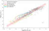 |
Fig. 6. L[C II–SFR relation for the three simulations used in this work (REF-L0025N0376, RECAL-L0025N0752, and REF-L0100N1504) presented as contour maps (pink, olive and cyan, respectively) and an observational sample of local galaxies (grey dots, briefly described in Appendix A). The contours shows where 90% (solid) and 50% (dashed) of the galaxies of the respective simulations fall in the relation. The sample of local galaxies is a compilation of different surveys containing main sequence galaxies (Brauher et al. 2008, ISO Compendium), starburst galaxies (Díaz-Santos et al. 2013, 2017, GOALS), dwarf galaxies (Cormier et al. 2015, 2019, HDGS), star-forming, AGN and LIRG galaxies (Herrera-Camus et al. 2018b,a, SHINING), dusty main sequence galaxies (Hughes et al. 2017, VALES) and intermediate-stellar-mass galaxies (Accurso et al. 2017, xCOLD GASS). We present the mean error from the observational samples in the bottom-right corner of the plot. The dashed red line is the power law derived by De Looze et al. (2014) for the relation at z = 0, with the shaded red region representing the 1σ scatter. |
The L[C II–SFR relation we inferred from the ISM model is presented in Fig. 6 and compared with selected samples of observed galaxies in the local Universe. We briefly describe the observational samples that we compare to in this paper in Appendix A. The multi-phase ISM model we have implemented in this work reproduces the observed galaxy distribution in the L[C II–SFR relation from De Looze et al. (2014, entire sample) and Pineda et al. (2014). In the range − 3.5 < log(SFR) [M⊙ yr−1] < 3, 77% of RECAL-L0025N0752 galaxies are inside the 1σ dispersion of the De Looze et al. (2014) relation. For the intermediate-resolution simulations (REF-L0025N0376 and REF-L0100N1504), only 47–60% of galaxies are inside the 1σ dispersion. If we compare with the 2σ dispersion around the De Looze et al. (2014) relation, we find 83, 95 and 96% of the galaxies inside the dispersion for REF-L0025N0376, REF-L0100N1504 and RECAL-L0025N0752, respectively. The dispersion (1σ) of the simulations (around 0.4 dex) is comparable to the De Looze et al. (2014) relation (0.42 dex). The typical statistical uncertainty in the observed SFR (L[C II) is around 10% (5%) but can go up to 40% (35%) in some cases (e.g., Cormier et al. 2015; Villanueva et al. 2017; Díaz-Santos et al. 2017).
The simulations underestimate the abundance of star-forming galaxies (1 − 10 M⊙ yr−1) in the local Universe due to the AGN feedback implementations used by EAGLE (Katsianis et al. 2017). In addition, the relatively small volume and physical prescriptions of the simulations (e.g., the IMF, lack of starburst galaxies and sub-grid physics) limit the comparison with luminous IR galaxies (e.g., (U)LIRGs) with SFR above 10 M⊙ yr−1 (Wang et al. 2019). Thus, the results of this work are mainly for galaxies with SFRs below 10 M⊙ yr−1. However, caution is need when comparing theoretical results with observational measurements as there could be important systematic differences. For example, the SFRs in EAGLE are computed from the KS law (Schaye & Dalla Vecchia 2008), while observational measurements of SFRs are normally based on IR luminosity.
Overall, Figs. 5 and 6 imply that in our simulated galaxies, the dominant phase of L[C II depends on the star-formation activity of the galaxy and the impact on each of the ISM phases can explain the shape of the L[C II–SFR relation (see discussions in Sects. 4.1 and 4.2). Although the simulations do not go to SFR ∼ 100 M⊙ yr−1, we can study the variations and trends of the physical parameters, which can provide some insights into the [C II] deficit (Sect. 4.2).
3.3. Pressure and metallicity dependence
To understand the origin of the L[C II–SFR relation, it is important to study how this relation varies as a function of other physical parameters. In this section, we study its dependence on pressure and metallicity.
We plot the L[C II/SFR ratio as a function of pressure in Fig. 7. We combine the three simulations. We bin the pressure and L[C II/SFR values with bin sizes determined using Knuth’s rule (Knuth 2006), which selects the simplest model that best describes the data by maximising the posterior probability for the number of bins. We colour-code the hexagonal bins by SFR in the range −2.5 < log(SFR) [M⊙ yr−1]< 1. We obtain similar results as Popping et al. (2019): At fixed SFR, the ratio of L[C II/SFR decreases with increasing pressure. This trend is expected as the mass-size relation of the neutral clouds in the model (Eq. (17)) depends on the pressure. At high pressure, the cloud is smaller and the emission region from the [C II] neutral phase decreases. We discuss the neutral cloud size dependency in Sect. 4.2.
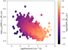 |
Fig. 7. L[C II/SFR ratio as a function of pressure, colour-coded by SFR. We present the mean value of SFR for each bin for the galaxies in the three simulations assuming they represent the same population. Pressure is anti-correlated with the L[C II/SFR ratio, in agreement with the result presented by Popping et al. (2019). We have confirmed that the trends do not depend on the specific simulation used. |
We used observational metallicity (12 + log(O/H)) values from the HDGS (Cormier et al. 2019), xCOLD GASS (Accurso et al. 2017) and VALES samples (taken from Zanella et al. 2018; Hughes et al. 2017). We converted LIR to SFR as described by Kennicutt & Evans (2012). As presented by Kewley & Ellison (2008), there is a large difference in the type of 12 + log(O/H) calibration used, in some cases up to 0.7 dex in log(O/H). For example, VALES and xCOLD GASS samples use the calibration from Pettini & Pagel (2004), while the HDGS sample uses a compilation of metallicities (Rémy-Ruyer et al. 2013). In this work, we do not calibrate the observations to a single metallicity calibration. In EAGLE, gas metallicity is defined as the fraction of the gas mass in elements heavier than helium. We use a solar metallicity of 12 + log(O/H) = 8.69 or Z = 0.0134 (Asplund et al. 2009) to compare EAGLE and observational values.
We show the variation of the L[C II/SFR ratio with metallicity for the three simulations in Fig. 8. There is no clear trend in the observational data, as we only have a few data points. The L[C II/SFR ratio in the simulations show a strong dependence on the mean gas metallicity values. Galaxies in REF-L0025N0376 and REF-L0100N1504 are located at higher values from the L[C II/SFR ratio compared to RECAL-L0025N0752 (as in Fig. 6), due to a higher contribution of the DIG phase (see discussion in Sect. 4.4). There is a decrease in the L[C II/SFR ratio from low metallicities up to 3 Z⊙ in galaxies in RECAL-L0025N0752. The total number of observed galaxies and simulated galaxies in the low-metallicity regime (below ∼0.2 Z⊙) is not enough to establish a clear trend between metallicity and L[C II/SFR as presented by Vallini et al. (2015) and Lupi & Bovino (2020), where there is an increase in the L[C II/SFR ratio with metallicity.
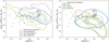 |
Fig. 8. L[C II/SFR ratio as a function of metallicity. Left panel: simulations compared with observed galaxies. Contours show where 90% (solid) and 50% (dashed) of the galaxies of the respective simulation lie. Right panel: the different ISM phases (DIG, atomic and molecular) in REF-L0100N1504. For the atomic phase, the L[C II/SFR increases with decreasing metallicity. For the molecular phase, it also decreases with increasing metallicity but plateaus at ∼1 Z⊙. For the DIG phase, it remains more or less constant. |
For metallicities higher than solar, we see a clear reduction in the L[C II/SFR ratio in REF-L0100N1504; therefore, we plot in the right panel of Fig. 8 the different ISM phases in REF-L0100N1504 as a function of metallicity. For the atomic phase, the L[C II/SFR ratio decreases with increasing metallicity. For the molecular phase, the ratio is more or less flat below solar metallicity, and then decreases with increasing metallicity above solar metallicity. On the other hand, the DIG is flat in the L[C II/SFR ratio at all metallicities. The decrease in the L[C II/SFR ratio at high metallicities can make a significant impact on the observed total L[C II when the atomic and molecular phases dominate L[C II. This probably results from higher radiation fields in metal-rich galaxies, which reduce the sizes of the neutral clouds, as proposed by Narayanan & Krumholz (2017). We find that galaxies with high metallicity have average neutral cloud sizes ∼30% smaller than metal-poor galaxies. We discuss this further in Sect. 4.
3.4. Spatial distributions
Finally, we check the spatial distribution of the ISM fractional contributions inside the galaxies. We calculate the distance between each phase to the centre of the potential in each galaxy. We scale the distance using the half-mass radius (R50) for all galaxies in REF-L0100N1504 from the EAGLE Database. We present the fractional contribution of the ISM phases against the distance from the centre in units of R50 in Fig. 9. These radial distributions of the fractional contributions to L[C II show that atomic gas dominates the luminosity contribution at the centres of the galaxies. The molecular phase never dominates, but the contribution peaks at r/R50 ≈ 0.5, while in the outskirts the DIG dominates.
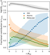 |
Fig. 9. Median radial distribution (diamonds) of the radiation field (grey) in the neutral clouds (upper panel) and the fractional ISM phase contributions (lower panel) for galaxies in REF-L0100N1504. There is a peak of neutral atomic gas contribution in the centre, the DIG contribution dominates beyond three times the half-mass radius (R50) of the galaxies, and the dense molecular gas contribution peaks around 0.5R50 and then decreases slowly. The peak of the radiation field is similar to the one of the dense molecular gas. Shaded colour shows the coverage between the 25th and 75th percentiles. |
The atomic and molecular phases are confined to the galaxy centres compared with the DIG. Atomic gas always dominates below R50, while the DIG median is nearly always lower than the molecular contribution within ∼R50. The DIG could be significant when L[C II is measured in observations of unresolved galaxies. As we show in Fig. 5, the contribution of each phase also depends on the SFR of the galaxy. At high SFR, the molecular fraction increases while the atomic contribution decreases. In the same way, the DIG dominates at low SFR, which will lead to a different radial distribution in less actively star-forming galaxies. However, we expect a similar trend where the fractional contributions of atomic and molecular gas peak at the centres of the galaxies and the DIG dominates in the outskirts.
4. Discussion
4.1. The role of the DIG in the [C II] emission of galaxies
One of the main conclusions we can draw from the ISM model implemented in this work is the role that the DIG plays in the production of L[C II. We show that the fractional contribution of each major ISM phase depends on the total SFR of the galaxy and the simulation used in Fig. 5. Intermediate-resolution simulations seem to overestimate the DIG contribution, while RECAL-L0025N0752 is consistent with previous studies in the local Universe (e.g., Pineda et al. 2014; Narayanan & Krumholz 2017; Croxall et al. 2017; Cormier et al. 2019; Lupi & Bovino 2020), where most of the [C II] emission arises from neutral phases (atomic and molecular). Figure 5 shows that when RECAL-L0025N0752 is used, the neutral phases dominate the L[C II fractional contribution, from around 60% at SFR ≈ 10−1 M⊙ yr−1 to 80% at SFR ≈ 10 M⊙ yr−1. Similar results are obtained when we look only at the inner parts of galaxies, inside R50 (Fig. 9). In galaxy centres, the total atomic contribution is ∼70% and the molecular contribution is ∼20%, while at R50 the atomic contribution is ∼45% and the molecular contribution is ∼30%.
The DIG is the dominant phase at metallicities above solar (∼70% of L[C II), at R50 ≳ 3, and in the low-SFR regime (< 10−2 M⊙ yr−1) in all three simulations. The L[C II],DIG/SFR ratio is more or less constant as a function of metallicity for the DIG phase (Fig. 8), in contrast to the atomic and molecular contributions, where the ratio is reduced drastically above solar metallicity. Below 1/3 Z⊙ the atomic gas is the dominant component in all three simulations (up to 90% at Z/Z⊙ = 0.03), while the contribution of the dense molecular gas peaks near to solar metallicity. Thus the DIG is the dominant contributor to L[C II in high-metallicity galaxies. These results support the trend presented by other works (Croxall et al. 2017; Cormier et al. 2019), where the fractional contribution of the DIG increases at high metallicities.
The radial position where the fractional contribution of the DIG is high corresponds to the outskirts of galaxies (Fig. 9). This agrees visually with the expected DIG location from Erroz-Ferrer et al. (2019, see their Appendix A), who estimated the location of the DIG regions, following a threshold value for the Hα emission (diffuse Hα emission), mainly in the outskirts of local star-forming galaxies. Although they do not compare Hα with [C II] emission, it is interesting to note the resemblance with another SFR tracer. This suggests that it could be possible to measure the DIG contribution in the outskirts of galaxies by measuring the [C II] flux, just like Hα emission. Croxall et al. (2017) and Sutter et al. (2019) found fractional contributions of DIG below 40% in resolved regions of galaxies, which coincide with our results inside the half-mass radii of galaxies (2–6 kpc). However, the results of Croxall et al. (2017) and Sutter et al. (2019) come mostly from regions within 0.25R256, limiting the interpretation of these studies on the spatial distribution of the DIG phase.
In an analytical study, Popping et al. (2019) assume a constant density for diffuse gas. When Popping et al. (2019) reduce the density of the diffuse gas, the total [C II] luminosity is more affected (up to 0.5 dex with respect to their fiducial model) at log(SFR) [M⊙ yr−1]< 0 than at log(SFR) [M⊙ yr−1]> 0 (their Fig. 15). This result is consistent with the trends found in our work. When the DIG dominates at low SFRs, even small changes in the DIG composition can affect the total [C II] luminosity. However, the assumption of a constant density for diffuse gas and other differences in the ISM models, limits a direct comparison of the DIG dependency on L[C II.
Our results show that, in metal-rich galaxies and where the SFR is low, the DIG could play a dominant role in producing the L[C II. Ignoring these contributions at different SFRs can introduce a bias in the line emission estimations (Croxall et al. 2017). Detailed resolved observations of local galaxies and their outskirts will be essential to improve the calibration of the DIG fraction. At the same time, observations of galaxies with low SFR will also be important.
4.2. Variations in the L[C II]–SFR relation
As mentioned in Sects. 1 and 3.2, one problem of using L[C II as a SFR indicator is that the L[C II–SFR relation is complex. A single power law cannot describe the relation accurately and variations are present due to changes in contribution from different ISM phases (Sects. 3.1 and 4.1) and the [C II] deficit, where the slope of L[C II with respect to FIR luminosity is less steep at high infrared luminosities.
A natural mechanism for the [C II] deficit was presented by Narayanan & Krumholz (2017), where the increase in the molecular fraction of the gas reduces the efficiency of [C II] emission due to the shrinking size of atomic gas in galaxies with high SFR. In Fig. 10, we present the average radius of the atomic region (Ratomic) in the simulated galaxies with respect to the total SFR, colour-coded by the average strength of the radiation field incident on the neutral cloud ( ). The plot shows a gradual decrease in the effective atomic radius with SFR, which can be related to
  . Ratomic shrinks because the sizes of the neutral clouds are reduced with increasing SFR, while RH2 increases. This explains the trends observed in Fig. 5, where the molecular fractional contribution rises after the peak contribution of the atomic gas.
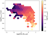 |
Fig. 10. Average radius of the atomic region (Ratomic) in all simulations (assuming they represent the same population) with respect to SFR, colour-coded by |


This result is not surprising as the SFR in the EAGLE simulations is determined by the pressure in the galaxy, and at the same time, pressure constrains the size of the neutral cloud, so these results reflect those of Narayanan & Krumholz (2017). Unfortunately, the evolution of Ratomic cannot be tested at higher SFR for the local Universe in EAGLE (Katsianis et al. 2017), but Ratomic is expected to decrease for systems with higher SFR.
Another claim related to the variations in the L[C II–SFR relation is that L[C II may not be a robust SFR indicator when intense radiation fields are present, such as in starburst galaxies (Herrera-Camus et al. 2018a; Ferrara et al. 2019). We test this hypothesis, following Herrera-Camus et al. (2018a), by calculating the specific star formation rate (sSFR = SFR/M⋆) for the galaxies in the simulations and normalising with the value derived for the main-sequence (MS) sSFR from Speagle et al. (2014). Figure 11 shows the L[C II/SFR ratio with respect to ΔMS. This result is similar to that presented by Herrera-Camus et al. (2018a, their Fig. 6) but lacking the starburst outliers (ΔMS ≳ 20), which are not reproduced by EAGLE. The Ratomic reduction and the decrease in L[C II/SFR ratio at higher ΔMS show that the strength of the radiation field can be a major factor in the observed variations in the L[C II–SFR relation.
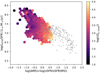 |
Fig. 11. L[C II/SFR ratio as a function of ΔMS for the three simulations (assuming they represent the same population), colour-coded by |

Díaz-Santos et al. (2017) show that less prominent [C II] deficits are related to higher [C II] fractional contributions coming from the neutral atomic phase. In Sutter et al. (2019) the main contributor to L[C II is found to be the neutral phase, which shows a less prominent [C II] deficit compared to the ionised phase. These results agree with those presented in this work. When the fractional contribution to L[C II from the atomic phase is small, the deficit is more prominent. The [C II] atomic phase contribution decreases at the same time that the total [C II] luminosity decreases. Thus the neutral phase is responsible for the deficit, as we have shown in this work.
However, when Sutter et al. (2019) consider only the ionised component, the [C II] deficit is more prominent compared to the neutral phases. This result is different from what we found in this work, where the [C II] luminosity from the DIG component does not decrease at the higher luminosities (logSFR ≈ 0.8 ∼ log LTIR ≈ 10.75 ) tested in this work. The methods used to calculate the ionised component may explain the differences between this work and Sutter et al. (2019). The Sutter et al. (2019) calculations come from directly scaling the [N II] 205 μM line deficit, while we calibrate the ionised component taking the two nitrogen emission lines and the SFR into account. The role that metallicity plays in the variation of the L[C II–SFR relation may also explain the differences. The sample of galaxies used by Sutter et al. (2019) has, in general, metallicities below solar. Our results (Fig. 8) show that in this range the atomic neutral phase dominates and the DIG contributes less at lower metallicities. In other words, this difference could be due to selection bias.
Smith et al. (2017) found a correlation between increased metallicity and deeper L[C II deficits in high-luminosity infrared galaxies. In our case, at higher metallicities, the atomic and molecular gas contributions to the L[C II seem to be more affected than the DIG contribution (Fig. 8), showing more prominent L[C II deficits. At values below solar metallicity, the structure of the ISM changes, especially the transition from WNM-to-CNM (Bialy & Sternberg 2019). In this work, at Z⊙< 1 the DIG seems to be deficient in producing [C II] compared to the atomic gas, but the DIG total contribution is always stable. As discussed in the previous paragraph, galaxies in the work by Sutter et al. (2019) and Díaz-Santos et al. (2017) are biased towards metallicities below solar, where atomic phases dominate L[C II.
The contribution of a given phase to the variations in L[C II–SFR relation depends on the star-formation regulation, due to AGN or star-formation feedback, and metallicity, and these are the keys to understanding the variations observed in line observations. However, we keep in mind that the observed variations in the L[C II–SFR relation can come from selection effects and other biases, such as galaxy brightness, where starburst systems are more easily observed due to their luminosity (Katz et al. 2019). Nonetheless, trends in theoretical models are also dependent on the assumed parameters to estimate line emission (e.g., Olsen et al. 2015, 2017; Vallini et al. 2013, 2015, 2017; Lagache et al. 2018; Cormier et al. 2019; Katz et al. 2019; Popping et al. 2019). We discuss the caveats of our choices in the following section.
4.3. Caveats on our predictions
4.3.1. Model assumptions
Our findings may be limited by the assumptions we made in Sect. 2.2. We use the model presented by Olsen et al. (2015, 2017) as a basis. However, we have important differences: We calculate the fraction of neutral hydrogen following Rahmati et al. (2013), we change the density distribution in the neutral clouds to a Plummer profile following Popping et al. (2019) and we calibrate the DIG using [N II] emission lines. The main weakness of our model is its geometric simplicity. The model is based on patches of gas (SPH particles) with assumed constant physical parameters, such as the metallicity, which limits comparisons with real galaxies, where the different ISM phases are entangled with each other (Olsen et al. 2018b). Recent observational results (Dessauges-Zavadsky et al. 2019) have shown that the neutral cloud mass function (Eq. (15)) is only valid in the local Universe but not at different redshifts, where neutral clouds could be more massive (higher surface densities). Fortunately, even though this simple approach does not take all galactic physics into account, the models reproduce observed relations in galaxies in the local Universe.
Olsen et al. (2018a) apply a geometrical correction to their predicted intensities because of the assumed spherical clouds in the model compared with the computed plane-parallel geometry coming from CLOUDY. We do not implement this correction because the effect of this correction is much smaller than the general scatter presented in Fig. 6; therefore, the computational effort of applying the correction is not justified.
4.3.2. DIG calibration
We calibrate the DIG emission (Sect. 2.2.3) to account for the luminosity coming from this ISM phase in the [C II] line. This approach is biased towards the physical properties of the observations used in the calibration, for example luminous galaxies. At the same time, the assumed distribution function for RDIG (Eq. (32)) is not entirely physically motivated, as we do not know the actual distribution of this ISM phase in different types of galaxies. As we show in Fig. 5, this calibration can affect the DIG contribution of the [C II] line. The spatial distribution presented in Fig. 9 could also be affected by the uncertainty of RDIG. With smaller (bigger) RDIG the density of the ionised clouds will increase (decrease), the gas becomes less (more) diffuse, thus the total luminosity coming from the DIG will increase (decrease) as well. However, the assumptions used in this work can give us insights into the general behaviour of the DIG (see the discussion in Sect. 4.4). Different physical assumptions for the DIG could be applied to the simulations, but most of them only assume the distribution of the ionised gas in disky galaxies (e.g., Haffner et al. 2009; Vandenbroucke & Wood 2019, and references therein). Models with reliably calibrated DIG properties would be very important to understand diagnostic line emissions in galaxy evolution (Kewley et al. 2019), and more observations focusing on this ISM phase are required, such as the GBT Diffuse Ionised Gas Survey7.
In this work, we present luminosity predictions coming from [C II] emission line with calibrated emission from [N II] emission lines, which is ideal in terms of modelling (Olsen et al. 2018b), as other lines can help to constrain the physical properties in the models to improve emission line predictions (Popping et al. 2019). We plan to study the local Universe and at high redshift with more FIR emission lines in future works.
4.4. Choice of simulation
The findings of this work may be somewhat limited by the selection of a given EAGLE simulation to estimate the line emission. For example, large cosmological volumes (L > 50 cMpc) provide a more representative range of environments in galaxies compared to small boxes (Schaye et al. 2015; Furlong et al. 2015). In addition, the efficiency of feedback must be calibrated (e.g., with the GSMF) in large hydrodynamical simulations where the ISM scales are unresolved, and therefore calibration is required to make valid predictions for observables (Schaye et al. 2015; Naab & Ostriker 2017).
We have presented results from three simulations (REF-L0025N0376, RECAL-L0025N0752, and REF-L0100N1504) to test the effects of the box size and resolution on the predictions. We presented some of these comparisons in Figs. 5–8. In terms of the simulated box size (REF-L0025N0376 vs REF-L0100N1504), the predictions are very similar, and only the total number, typical masses and SFR of galaxies change. As remarked above, EAGLE does not contain many galaxies with SFR > 1 M⊙ yr−1 at z = 0 due to the specific implementations (Katsianis et al. 2017; Wang et al. 2019); therefore, with EAGLE simulations we can predict line emissions for normal star-forming galaxies at z = 0, but not starburst-like systems.
The trends in Figs. 6 and 8 show that L[C II is always lower for RECAL-L0025N0752 galaxies. These lower values are due to the GSMF re-calibration. De Rossi et al. (2017) noted that the increase in the resolution for these simulations (REF-L0100N1504 to RECAL-L0025N0752) can affect some features but the fundamental metallicity scaling relations are not altered. Therefore, boxes re-calibrated to the GSMF are a good starting point to predicting emission lines as metallicity scaling relations holds. From our comparison with observations (Sect. 3.1), we expect that the observed galaxies in the local Universe behave as in RECAL-L0025N0752, where the atomic gas dominates at SFR values higher than 0.01 M⊙ yr−1.
REF-L0100N1504 provides (statistical) clues on how the fractional contribution of the ISM phases changes. Predicted luminosities from REF-L0100N1504 and REF-L0025N0376 are overestimated compared with observed galaxies, which are well reproduced by RECAL-L0025N0752. This conclusion can also be seen from the right panel of Fig. 8, where a reduction of the contribution from atomic and molecular phases in L[C II increases the dominance of the DIG phase. To summarise, RECAL-L0025N0752 gives us the best predictions in terms of reproducing observed local galaxies and REF-L0100N1504 gives us larger sample sizes for statistical studies.
As RECAL-L0025N0752 does not reproduce the large number of galaxies needed for some statistical studies, we suggest that the best way to compare our simulations to observations is a mix between REF-L0100N1504 and RECAL-L0025N0752 to observe the global behaviour of the emission lines, as we do in Figs. 10 and 11. This gives us a better idea of the contribution of the different ISM phases to the line emission.
5. Summary and conclusions
In this work, we have post-processed SPH EAGLE simulations using a multi-phase ISM model and then predicted the luminosity of [C II] emission at 158 μm with CLOUDY. We set out to determine the fractional contributions of the different ISM phases to the [C II] line and the effect of these phases on the L[C II–SFR relation. We use three sets of simulations (REF-L0025N0376, RECAL-L0025N0752, and REF-L0100N1504) with two CLOUDY cooling tables for shielded and optically thin regimes (Ploeckinger & Schaye 2020) to characterise ISM composition in terms of dense molecular gas, neutral atomic gas, and diffuse ionised gas (DIG). We validate our model by comparing with observations of local galaxies. Our main conclusions are the following:
-
We find a dependence of the fractional contribution of the different ISM phases to L[C II on the total SFR and metallicity. Our model agrees with previous works where the [C II] emission comes mainly from neutral ISM regions in observed galaxies. However, this could be a selection bias in the observations towards galaxies with metallicities below solar.
-
In systems where the SFR is low, the DIG plays a dominant role in producing L[C II. Additional resolved observations of local galaxies with low SFRs and their outskirts will be essential to improve the calibration of the DIG fraction in other emission lines (van der Tak et al. 2018).
-
The model for the ISM we have implemented in this work reproduces the observed L[C II–SFR relation in local galaxies, although this result depends on calibrating the DIG with [N II] emission lines.
-
Star-formation regulation and metallicity dependence of the different ISM phases could be responsible for the variations observed in L[C II at high infrared luminosities, based on the dependence on ΔMS and average Rcloud. Further investigations are needed to verify if this result holds at higher redshifts.
-
The use of large boxes (box-size ≳100 cMpc) and high-resolution simulations (mass resolution ≲105 M⊙) is key to correctly predict emission lines in different types of galaxies.
In the future, we will take black hole particles (especially the SMBH) into account, which will alter the radiation field in the centres of the galaxies. We will use a random sample of galaxies from the simulations to estimate other fine structure lines. We plan to compare predictions in high-redshift systems with observational results, such as those presented by Le Fèvre et al. (2020) and Neeleman et al. (2019) with a large8 number of observed galaxies, using for example ΔMS.
We adopted the Geneva stellar models (Schaller et al. 1992) with standard mass loss.
The star formation time t* is used to calculate the age of the stars (i.e. lookback time).
The optically thick and optically thin tables are the UVB_dust1_CR1_G1_shield1 and UVB_dust1_CR1_G1_shield0 in Ploeckinger & Schaye (2020), respectively.
1/8 of the D25 standard diameter, the B-band isophotal radius at 25 mag arcsec−2 (de Vaucouleurs et al. 1991; Paturel et al. 1991; Prugniel & Heraudeau 1998).
Acknowledgments
The authors thank Rodrigo Herrera-Camus for providing the data from the SHINING survey. We acknowledge the anonymous referee for a careful reading of the manuscript and very helpful questions and comments. We acknowledge the Virgo Consortium for making their simulation data available. The EAGLE simulations were performed using the DiRAC-2 facility at Durham, managed by the ICC, and the PRACE facility Curie based in France at TGCC, CEA, Bruyères-le-Châtel. This research made use of Astropy, a community-developed core Python package for Astronomy (Astropy Collaboration 2013, 2018). We would like to thank the Center for Information Technology of the University of Groningen for their support and for providing access to the Peregrine high performance computing cluster.
References
- Abdullah, A., & Tielens, A. G. G. M. 2020, A&A, 639, A110 [CrossRef] [EDP Sciences] [Google Scholar]
- Abdullah, A., Brandl, B. R., Groves, B., et al. 2017, ApJ, 842, 4 [NASA ADS] [CrossRef] [Google Scholar]
- Accurso, G., Saintonge, A., Catinella, B., et al. 2017, MNRAS, 470, 4750 [NASA ADS] [Google Scholar]
- Arata, S., Yajima, H., Nagamine, K., Abe, M., & Khochfar, S. 2020, MNRAS, 498, 5541 [NASA ADS] [CrossRef] [Google Scholar]
- Asplund, M., Grevesse, N., Sauval, A. J., & Scott, P. 2009, ARA&A, 47, 481 [NASA ADS] [CrossRef] [Google Scholar]
- Astropy Collaboration (Robitaille, T. P., et al.) 2013, A&A, 558, A33 [NASA ADS] [CrossRef] [EDP Sciences] [Google Scholar]
- Astropy Collaboration (Price-Whelan, A. M., et al.) 2018, AJ, 156, 123 [Google Scholar]
- Bakx, T. J. L. C., Tamura, Y., Hashimoto, T., et al. 2020, MNRAS, 493, 4294 [NASA ADS] [CrossRef] [Google Scholar]
- Bethermin, M., Fudamoto, Y., Ginolfi, M., et al. 2020, A&A, 643, A2 [CrossRef] [EDP Sciences] [Google Scholar]
- Bialy, S., & Sternberg, A. 2019, ApJ, 881, 160 [NASA ADS] [CrossRef] [Google Scholar]
- Black, J. H. 1987, in Heating and Cooling of the Interstellar Gas, eds. D. J. Hollenbach, J. Thronson, & A. Harley, 134, 731 [Google Scholar]
- Blitz, L., Fukui, Y., Kawamura, A., et al. 2007, in Protostars and Planets V, eds. B. Reipurth, D. Jewitt, K. Keil, et al., 81 [Google Scholar]
- Bolatto, A. D., Leroy, A. K., Rosolowsky, E., Walter, F., & Blitz, L. 2008, ApJ, 686, 948 [NASA ADS] [CrossRef] [Google Scholar]
- Bonatto, C., & Bica, E. 2011, MNRAS, 415, 2827 [NASA ADS] [CrossRef] [Google Scholar]
- Brauher, J. R., Dale, D. A., & Helou, G. 2008, ApJS, 178, 280 [NASA ADS] [CrossRef] [Google Scholar]
- Carniani, S., Maiolino, R., Pallottini, A., et al. 2017, A&A, 605, A42 [NASA ADS] [CrossRef] [EDP Sciences] [Google Scholar]
- Cole, S., Lacey, C. G., Baugh, C. M., & Frenk, C. S. 2000, MNRAS, 319, 168 [NASA ADS] [CrossRef] [Google Scholar]
- Cormier, D., Lebouteiller, V., Madden, S. C., et al. 2012, A&A, 548, A20 [NASA ADS] [CrossRef] [EDP Sciences] [Google Scholar]
- Cormier, D., Madden, S. C., Lebouteiller, V., et al. 2015, A&A, 578, A53 [NASA ADS] [CrossRef] [EDP Sciences] [Google Scholar]
- Cormier, D., Abel, N. P., Hony, S., et al. 2019, A&A, 626, A23 [NASA ADS] [CrossRef] [EDP Sciences] [Google Scholar]
- Cowie, L. L., Songaila, A., Hu, E. M., & Cohen, J. G. 1996, AJ, 112, 839 [Google Scholar]
- Crain, R. A., Schaye, J., Bower, R. G., et al. 2015, MNRAS, 450, 1937 [NASA ADS] [CrossRef] [Google Scholar]
- Croton, D. J., Springel, V., White, S. D. M., et al. 2006, MNRAS, 365, 11 [NASA ADS] [CrossRef] [Google Scholar]
- Croxall, K. V., Smith, J. D., Pellegrini, E., et al. 2017, ApJ, 845, 96 [NASA ADS] [CrossRef] [Google Scholar]
- Dalla Vecchia, C., & Schaye, J. 2012, MNRAS, 426, 140 [NASA ADS] [CrossRef] [Google Scholar]
- Dayal, P., & Ferrara, A. 2018, Phys. Rep., 780, 1 [NASA ADS] [CrossRef] [Google Scholar]
- De Looze, I., Baes, M., Bendo, G. J., Cortese, L., & Fritz, J. 2011, MNRAS, 416, 2712 [Google Scholar]
- De Looze, I., Cormier, D., Lebouteiller, V., et al. 2014, A&A, 568, A62 [NASA ADS] [CrossRef] [EDP Sciences] [Google Scholar]
- De Rossi, M. E., Bower, R. G., Font, A. S., Schaye, J., & Theuns, T. 2017, MNRAS, 472, 3354 [NASA ADS] [CrossRef] [Google Scholar]
- de Vaucouleurs, G., de Vaucouleurs, A., Corwin, H. G. J. et al. 1991, Third Reference Catalogue of Bright Galaxies (New York: Springer) [Google Scholar]
- Dessauges-Zavadsky, M., Richard, J., Combes, F., et al. 2019, Nat. Astron., 3, 1114 [CrossRef] [Google Scholar]
- Díaz-Santos, T., Armus, L., Charmandaris, V., et al. 2013, ApJ, 774, 68 [NASA ADS] [CrossRef] [Google Scholar]
- Díaz-Santos, T., Armus, L., Charmandaris, V., et al. 2017, ApJ, 846, 32 [Google Scholar]
- Dolag, K., Borgani, S., Murante, G., & Springel, V. 2009, MNRAS, 399, 497 [Google Scholar]
- Elmegreen, B. G. 1989, ApJ, 344, 306 [NASA ADS] [CrossRef] [Google Scholar]
- Erroz-Ferrer, S., Carollo, C. M., den Brok, M., et al. 2019, MNRAS, 484, 5009 [NASA ADS] [CrossRef] [Google Scholar]
- Faesi, C. M., Lada, C. J., & Forbrich, J. 2018, ApJ, 857, 19 [NASA ADS] [CrossRef] [Google Scholar]
- Fahrion, K., Cormier, D., Bigiel, F., et al. 2017, A&A, 599, A9 [NASA ADS] [CrossRef] [EDP Sciences] [Google Scholar]
- Faucher-Giguère, C.-A. 2020, MNRAS, 493, 1614 [CrossRef] [Google Scholar]
- Ferland, G. J., Korista, K. T., Verner, D. A., et al. 1998, PASP, 110, 761 [Google Scholar]
- Ferland, G. J., Porter, R. L., van Hoof, P. A. M., et al. 2013, Rev. Mex. Astron. Astrofis., 49, 137 [Google Scholar]
- Ferland, G. J., Chatzikos, M., Guzmán, F., et al. 2017, Rev. Mex. Astron. Astrofis., 53, 385 [NASA ADS] [Google Scholar]
- Fernández-Ontiveros, J. A., Spinoglio, L., Pereira-Santaella, M., et al. 2016, ApJS, 226, 19 [NASA ADS] [CrossRef] [Google Scholar]
- Ferrara, A., Vallini, L., Pallottini, A., et al. 2019, MNRAS, 489, 1 [NASA ADS] [CrossRef] [Google Scholar]
- Field, G. B., Blackman, E. G., & Keto, E. R. 2011, MNRAS, 416, 710 [NASA ADS] [Google Scholar]
- Furlong, M., Bower, R. G., Theuns, T., et al. 2015, MNRAS, 450, 4486 [Google Scholar]
- Gnedin, N. Y., & Kravtsov, A. V. 2011, ApJ, 728, 88 [NASA ADS] [CrossRef] [MathSciNet] [Google Scholar]
- Goldsmith, P. F., Langer, W. D., Pineda, J. L., & Velusamy, T. 2012, ApJS, 203, 13 [Google Scholar]
- Gong, Y., Cooray, A., Silva, M., et al. 2012, ApJ, 745, 49 [NASA ADS] [CrossRef] [Google Scholar]
- Gullberg, B., De Breuck, C., Vieira, J. D., et al. 2015, MNRAS, 449, 2883 [Google Scholar]
- Habing, H. J. 1968, Bull. Astron. Inst. Netherlands, 19, 421 [Google Scholar]
- Haffner, L. M., Dettmar, R. J., Beckman, J. E., et al. 2009, Rev. Mod. Phys., 81, 969 [NASA ADS] [CrossRef] [Google Scholar]
- Haines, C. P., Iovino, A., Krywult, J., et al. 2017, A&A, 605, A4 [NASA ADS] [CrossRef] [EDP Sciences] [Google Scholar]
- Herrera-Camus, R., Bolatto, A. D., Wolfire, M. G., et al. 2015, ApJ, 800, 1 [Google Scholar]
- Herrera-Camus, R., Sturm, E., Graciá-Carpio, J., et al. 2018a, ApJ, 861, 95 [Google Scholar]
- Herrera-Camus, R., Sturm, E., Graciá-Carpio, J., et al. 2018b, ApJ, 861, 94 [NASA ADS] [CrossRef] [Google Scholar]
- Hollenbach, D. J., & Tielens, A. G. G. M. 1999, Rev. Mod. Phys., 71, 173 [Google Scholar]
- Hopkins, P. F. 2013, MNRAS, 428, 2840 [NASA ADS] [CrossRef] [Google Scholar]
- Hopkins, P. F., Kereš, D., Oñorbe, J., et al. 2014, MNRAS, 445, 581 [NASA ADS] [CrossRef] [Google Scholar]
- Hughes, A., Meidt, S. E., Colombo, D., et al. 2013, ApJ, 779, 46 [NASA ADS] [CrossRef] [EDP Sciences] [Google Scholar]
- Hughes, T. M., Ibar, E., Villanueva, V., et al. 2017, A&A, 602, A49 [NASA ADS] [CrossRef] [EDP Sciences] [Google Scholar]
- Hui, L., & Gnedin, N. Y. 1997, MNRAS, 292, 27 [Google Scholar]
- Indriolo, N., Geballe, T. R., Oka, T., & McCall, B. J. 2007, ApJ, 671, 1736 [NASA ADS] [CrossRef] [Google Scholar]
- Inoue, A. K., Tamura, Y., Matsuo, H., et al. 2016, Science, 352, 1559 [NASA ADS] [CrossRef] [Google Scholar]
- Jenkins, E. B. 2009, ApJ, 700, 1299 [NASA ADS] [CrossRef] [Google Scholar]
- Katsianis, A., Blanc, G., Lagos, C. P., et al. 2017, MNRAS, 472, 919 [NASA ADS] [CrossRef] [Google Scholar]
- Katz, H., Kimm, T., Sijacki, D., & Haehnelt, M. G. 2017, MNRAS, 468, 4831 [NASA ADS] [CrossRef] [Google Scholar]
- Katz, H., Galligan, T. P., Kimm, T., et al. 2019, MNRAS, 487, 5902 [NASA ADS] [CrossRef] [Google Scholar]
- Kaufman, M. J., Wolfire, M. G., Hollenbach, D. J., & Luhman, M. L. 1999, ApJ, 527, 795 [Google Scholar]
- Kennicutt, R. C., & Evans, N. J. 2012, ARA&A, 50, 531 [NASA ADS] [CrossRef] [Google Scholar]
- Kewley, L. J., & Ellison, S. L. 2008, ApJ, 681, 1183 [Google Scholar]
- Kewley, L. J., Nicholls, D. C., & Sutherland, R. S. 2019, ARA&A, 57, 511 [Google Scholar]
- Knudsen, K. K., Richard, J., Kneib, J.-P., et al. 2016, MNRAS, 462, L6 [NASA ADS] [CrossRef] [Google Scholar]
- Knuth, K. H. 2006, ArXiv e-prints [arXiv:physics/0605197] [Google Scholar]
- Lagache, G., Cousin, M., & Chatzikos, M. 2018, A&A, 609, A130 [NASA ADS] [CrossRef] [EDP Sciences] [Google Scholar]
- Lagos, C. d. P., Crain, R. A., Schaye, J., et al. 2015, MNRAS, 452, 3815 [CrossRef] [Google Scholar]
- Le Fèvre, O., Béthermin, M., Faisst, A., et al. 2020, A&A, 643, A1 [CrossRef] [EDP Sciences] [Google Scholar]
- Leitherer, C., Ekström, S., Meynet, G., et al. 2014, ApJS, 212, 14 [NASA ADS] [CrossRef] [Google Scholar]
- Lupi, A., & Bovino, S. 2020, MNRAS, 492, 2818 [Google Scholar]
- Lupi, A., Pallottini, A., Ferrara, A., et al. 2020, MNRAS, 496, 5160 [Google Scholar]
- Maiolino, R., Carniani, S., Fontana, A., et al. 2015, MNRAS, 452, 54 [NASA ADS] [CrossRef] [Google Scholar]
- Malhotra, S., Kaufman, M. J., Hollenbach, D., et al. 2001, ApJ, 561, 766 [Google Scholar]
- McAlpine, S., Helly, J. C., Schaller, M., et al. 2016, Astron. Comput., 15, 72 [NASA ADS] [CrossRef] [Google Scholar]
- Mezger, P. G., Mathis, J. S., & Panagia, N. 1982, A&A, 105, 372 [NASA ADS] [Google Scholar]
- Miville-Deschênes, M.-A., Murray, N., & Lee, E. J. 2017, ApJ, 834, 57 [NASA ADS] [CrossRef] [Google Scholar]
- Moriwaki, K., Yoshida, N., Shimizu, I., et al. 2018, MNRAS, 481, L84 [NASA ADS] [CrossRef] [Google Scholar]
- Muñoz, J. A., & Oh, S. P. 2016, MNRAS, 463, 2085 [NASA ADS] [CrossRef] [Google Scholar]
- Murray, N. 2011, ApJ, 729, 133 [NASA ADS] [CrossRef] [Google Scholar]
- Naab, T., & Ostriker, J. P. 2017, ARA&A, 55, 59 [Google Scholar]
- Nagamine, K., Wolfe, A. M., & Hernquist, L. 2006, ApJ, 647, 60 [NASA ADS] [CrossRef] [Google Scholar]
- Narayanan, D., Cox, T. J., Kelly, B., et al. 2008a, ApJS, 176, 331 [NASA ADS] [CrossRef] [Google Scholar]
- Narayanan, D., Cox, T. J., Shirley, Y., et al. 2008b, ApJ, 684, 996 [NASA ADS] [CrossRef] [Google Scholar]
- Narayanan, D., & Krumholz, M. R. 2017, MNRAS, 467, 50 [NASA ADS] [CrossRef] [Google Scholar]
- Neeleman, M., Bañados, E., Walter, F., et al. 2019, ApJ, 882, 10 [NASA ADS] [CrossRef] [Google Scholar]
- Olsen, K. P., Greve, T. R., Narayanan, D., et al. 2015, ApJ, 814, 76 [CrossRef] [Google Scholar]
- Olsen, K., Greve, T. R., Narayanan, D., et al. 2017, ApJ, 846, 105 [NASA ADS] [CrossRef] [Google Scholar]
- Olsen, K., Greve, T. R., Narayanan, D., et al. 2018a, ApJ, 857, 148 [NASA ADS] [CrossRef] [Google Scholar]
- Olsen, K., Pallottini, A., Wofford, A., et al. 2018b, Galaxies, 6, 100 [NASA ADS] [CrossRef] [Google Scholar]
- Oteo, I., Zwaan, M. A., Ivison, R. J., Smail, I., & Biggs, A. D. 2017, ApJ, 837, 182 [NASA ADS] [CrossRef] [Google Scholar]
- Pallottini, A., Ferrara, A., Bovino, S., et al. 2017a, MNRAS, 471, 4128 [NASA ADS] [CrossRef] [Google Scholar]
- Pallottini, A., Ferrara, A., Gallerani, S., et al. 2017b, MNRAS, 465, 2540 [NASA ADS] [CrossRef] [Google Scholar]
- Paturel, G., Fouqué, P., Buta, R., & Garcia, A. M. 1991, A&A, 243, 319 [Google Scholar]
- Pelupessy, F. I., & Papadopoulos, P. P. 2009, ApJ, 707, 954 [NASA ADS] [CrossRef] [Google Scholar]
- Pentericci, L., Carniani, S., Castellano, M., et al. 2016, ApJ, 829, L11 [NASA ADS] [CrossRef] [Google Scholar]
- Pérez-González, P. G., Rieke, G. H., Villar, V., et al. 2008, ApJ, 675, 234 [NASA ADS] [CrossRef] [Google Scholar]
- Pettini, M., & Pagel, B. E. J. 2004, MNRAS, 348, L59 [NASA ADS] [CrossRef] [Google Scholar]
- Pillepich, A., Springel, V., Nelson, D., et al. 2018, MNRAS, 473, 4077 [Google Scholar]
- Pineda, J. L., Langer, W. D., Velusamy, T., & Goldsmith, P. F. 2013, A&A, 554, A103 [NASA ADS] [CrossRef] [EDP Sciences] [Google Scholar]
- Pineda, J. L., Langer, W. D., & Goldsmith, P. F. 2014, A&A, 570, A121 [NASA ADS] [CrossRef] [EDP Sciences] [Google Scholar]
- Pineda, J. L., Fischer, C., Kapala, M., et al. 2018, ApJ, 869, L30 [CrossRef] [Google Scholar]
- Planck Collaboration I. 2014, A&A, 571, A1 [NASA ADS] [CrossRef] [EDP Sciences] [Google Scholar]
- Planck Collaboration XVI. 2014, A&A, 571, A16 [NASA ADS] [CrossRef] [EDP Sciences] [Google Scholar]
- Planck Collaboration XIII. 2016, A&A, 594, A13 [NASA ADS] [CrossRef] [EDP Sciences] [Google Scholar]
- Ploeckinger, S., & Schaye, J. 2020, MNRAS, 497, 4857 [CrossRef] [Google Scholar]
- Popping, G., Narayanan, D., Somerville, R. S., Faisst, A. L., & Krumholz, M. R. 2019, MNRAS, 482, 4906 [Google Scholar]
- Prugniel, P., & Heraudeau, P. 1998, A&AS, 128, 299 [NASA ADS] [CrossRef] [EDP Sciences] [Google Scholar]
- Rahmati, A., Pawlik, A. H., Raičević, M., & Schaye, J. 2013, MNRAS, 430, 2427 [NASA ADS] [CrossRef] [Google Scholar]
- Rémy-Ruyer, A., Madden, S. C., Galliano, F., et al. 2013, A&A, 557, A95 [NASA ADS] [CrossRef] [EDP Sciences] [Google Scholar]
- Robitaille, T. P., & Whitney, B. A. 2010, ApJ, 710, L11 [NASA ADS] [CrossRef] [Google Scholar]
- Röllig, M., Ossenkopf, V., Jeyakumar, S., Stutzki, J., & Sternberg, A. 2006, A&A, 451, 917 [NASA ADS] [CrossRef] [EDP Sciences] [Google Scholar]
- Rosas-Guevara, Y. M., Bower, R. G., Schaye, J., et al. 2015, MNRAS, 454, 1038 [CrossRef] [Google Scholar]
- Saintonge, A., Catinella, B., Cortese, L., et al. 2016, MNRAS, 462, 1749 [Google Scholar]
- Schaller, G., Schaerer, D., Meynet, G., & Maeder, A. 1992, A&AS, 96, 269 [Google Scholar]
- Schaye, J. 2001, ApJ, 559, 507 [NASA ADS] [CrossRef] [Google Scholar]
- Schaye, J., & Dalla Vecchia, C. 2008, MNRAS, 383, 1210 [NASA ADS] [CrossRef] [EDP Sciences] [Google Scholar]
- Schaye, J., Crain, R. A., Bower, R. G., et al. 2015, MNRAS, 446, 521 [Google Scholar]
- Seon, K.-I., Edelstein, J., Korpela, E., et al. 2011, ApJS, 196, 15 [NASA ADS] [CrossRef] [Google Scholar]
- Shaw, G., Ferland, G. J., & Ploeckinger, S. 2020, Res. Notes Am. Astron. Soc., 4, 78 [CrossRef] [Google Scholar]
- Smith, J. D. T., Croxall, K., Draine, B., et al. 2017, ApJ, 834, 5 [NASA ADS] [CrossRef] [Google Scholar]
- Somerville, R. S., & Davé, R. 2015, ARA&A, 53, 51 [Google Scholar]
- Somerville, R. S., & Primack, J. R. 1999, MNRAS, 310, 1087 [CrossRef] [Google Scholar]
- Speagle, J. S., Steinhardt, C. L., Capak, P. L., & Silverman, J. D. 2014, ApJS, 214, 15 [NASA ADS] [CrossRef] [Google Scholar]
- Spilker, J. S., Marrone, D. P., Aravena, M., et al. 2016, ApJ, 826, 112 [NASA ADS] [CrossRef] [Google Scholar]
- Springel, V., White, S. D. M., Tormen, G., & Kauffmann, G. 2001, MNRAS, 328, 726 [Google Scholar]
- Springel, V., Di Matteo, T., & Hernquist, L. 2005, MNRAS, 361, 776 [Google Scholar]
- Stacey, G. J., Geis, N., Genzel, R., et al. 1991, ApJ, 373, 423 [NASA ADS] [CrossRef] [Google Scholar]
- Stacey, G. J., Hailey-Dunsheath, S., Ferkinhoff, C., et al. 2010, ApJ, 724, 957 [NASA ADS] [CrossRef] [Google Scholar]
- Sutter, J., Dale, D. A., Croxall, K. V., et al. 2019, ApJ, 886, 60 [NASA ADS] [CrossRef] [Google Scholar]
- The EAGLE team 2017, ArXiv e-prints [arXiv:1706.09899] [Google Scholar]
- Theuns, T., Leonard, A., Efstathiou, G., Pearce, F. R., & Thomas, P. A. 1998, MNRAS, 301, 478 [NASA ADS] [CrossRef] [Google Scholar]
- Thob, A. C. R., Crain, R. A., McCarthy, I. G., et al. 2019, MNRAS, 485, 972 [Google Scholar]
- Tielens, A. G. G. M., & Hollenbach, D. 1985, ApJ, 291, 722 [NASA ADS] [CrossRef] [Google Scholar]
- Tress, R. G., Smith, R. J., Sormani, M. C., et al. 2020a, MNRAS, 492, 2973 [Google Scholar]
- Tress, R. G., Sormani, M. C., Glover, S. C. O., et al. 2020b, MNRAS, 499, 4455 [CrossRef] [Google Scholar]
- Vallini, L., Gallerani, S., Ferrara, A., & Baek, S. 2013, MNRAS, 433, 1567 [NASA ADS] [CrossRef] [Google Scholar]
- Vallini, L., Gallerani, S., Ferrara, A., Pallottini, A., & Yue, B. 2015, ApJ, 813, 36 [NASA ADS] [CrossRef] [Google Scholar]
- Vallini, L., Ferrara, A., Pallottini, A., & Gallerani, S. 2017, MNRAS, 467, 1300 [NASA ADS] [Google Scholar]
- van der Tak, F. F. S., Madden, S. C., Roelfsema, P., et al. 2018, PASA, 35, e002 [NASA ADS] [CrossRef] [Google Scholar]
- Vandenbroucke, B., & Wood, K. 2019, MNRAS, 488, 1977 [NASA ADS] [CrossRef] [Google Scholar]
- Villanueva, V., Ibar, E., Hughes, T. M., et al. 2017, MNRAS, 470, 3775 [NASA ADS] [CrossRef] [Google Scholar]
- Vogelsberger, M., Genel, S., Springel, V., et al. 2014, MNRAS, 444, 1518 [NASA ADS] [CrossRef] [Google Scholar]
- Wang, L., Pearson, W. J., Cowley, W., et al. 2019, A&A, 624, A98 [CrossRef] [EDP Sciences] [Google Scholar]
- Wiersma, R. P. C., Schaye, J., & Smith, B. D. 2009a, MNRAS, 393, 99 [NASA ADS] [CrossRef] [Google Scholar]
- Wiersma, R. P. C., Schaye, J., Theuns, T., Dalla Vecchia, C., & Tornatore, L. 2009b, MNRAS, 399, 574 [NASA ADS] [CrossRef] [Google Scholar]
- Wolfire, M. G., Hollenbach, D., McKee, C. F., Tielens, A. G. G. M., & Bakes, E. L. O. 1995, ApJ, 443, 152 [Google Scholar]
- Wolfire, M. G., McKee, C. F., Hollenbach, D., & Tielens, A. G. G. M. 2003, ApJ, 587, 278 [NASA ADS] [CrossRef] [Google Scholar]
- Zanella, A., Daddi, E., Magdis, G., et al. 2018, MNRAS, 481, 1976 [Google Scholar]
Appendix A: Comments on archival Data
To complement and verify our model in the local Universe, we use archival data from different samples of observed galaxies where the [C II] luminosity is available. In cases where it is possible, we recalculate the luminosities and SFRs with the same cosmology used in this work (Planck Collaboration I 2014). We use the literature samples from (a) the ISO compendium (Brauher et al. 2008) of main-sequence galaxies; (b) xCOLD GASS (Accurso et al. 2017), composed of intermediate-stellar-mass galaxies; (c) GOALS (Díaz-Santos et al. 2013, 2017), composed of LIRGS observed with Spitzer and Herschel; (d) SHINING (Herrera-Camus et al. 2018a), composed of nearby star-forming galaxies, AGNs, and LIRGs observed with Herschel; (e) VALES (Hughes et al. 2017), composed of dusty main-sequence star-forming galaxies observed with ALMA; and (f) the Herschel Dwarf Galaxy Survey (HDGS, Cormier et al. 2015, 2019). For the ISO compendium: We ignore close galaxies (below 1 Mpc), we use the median for the line flux in galaxies with more than one measure in the [C II] line, and the infrared luminosity was calculated with the 60 and 100 μm from the IRAS flux as described by Brauher et al. (2008). In most of the literature samples we have calculated the SFR from the IR luminosity as described by Kennicutt & Evans (2012). We use the SFRs from Villanueva et al. (2017) and Saintonge et al. (2016) for VALES and xCOLD GASS samples, respectively.
We compare these literature samples with our SFR and L[C II estimates in Fig. A.1. We notice that galaxies in RECAL-L0025N0752 follow similar trend as the dwarf galaxies from Cormier et al. (2019) while REF-L0100N1504 is similar to most of the intermediate stellar mass galaxies from Accurso et al. (2017). Both simulations reproduce main sequence galaxies (Brauher et al. 2008) as well as some galaxies from other samples (e.g., Hughes et al. 2017; Herrera-Camus et al. 2018a). LIRGS galaxies (Díaz-Santos et al. 2017; Herrera-Camus et al. 2018a) are representative of the [C II] deficit, but unfortunately, are not recovered by EAGLE (see Sect. 3.2 and Fig. 6 to compare with the deficit).
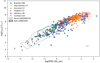 |
Fig. A.1. L[C II–SFR relation for the observational sample of local galaxies and two simulations used in this work (RECAL-L0025N0752, REF-L0100N1504) presented as contour maps (grey and black). The contours shows where 95% of the galaxies of the respective simulations fall in the relation. We present the mean error from the observational samples in the bottom-right corner of the plot. |
Additionally, we use [N II] observational data from Fernández-Ontiveros et al. (2016) to calibrate the DIG. We describe the procedure in Sect. 2.2.3 and in Fig. 1 we show the simulated and observed L[N II]–SFR relation for the lines at 122 and 205 μm.
All Tables
All Figures
|
Fig. 1. L[N II]122–SFR (left) and L[N II]205–SFR (right) relations for the three simulations used (REF-L0025N0376, RECAL-L0025N0752, and REF-L0100N1504) and the observational sample used for the DIG calibration from Fernández-Ontiveros et al. (2016) (grey dots). The smoothed contours show where 90% (solid) and 50% (dashed) of the galaxies from the respective simulations lie. The remaining 10% of galaxies are represented as dots using the same colours. |
| In the text | |
|
Fig. 2. Flowchart of the sub-grid procedures applied to the SPH simulation to simulate line emission in post-processing. For each EAGLE simulation, we obtain the galaxy information from the database and we use the star and gas particle data to implement the ISM model. Next, we calculate physical properties in each phase to obtain the neutral clouds and DIG structures. We use CLOUDY cooling tables (Ploeckinger & Schaye 2020) to get the line luminosity for [C II]. We first calculate L[C II],DIG and then calibrate the ionised gas using the predicted luminosities of the [N II] lines. We then obtain the total line luminosity from the luminosities of the different ISM phases. The dashed lines connect the gas environment to the ingredients of the model. |
| In the text | |
|
Fig. 3. Mean mass-weighted distribution of the sizes of the ISM phases for RECAL-L0025N0752. Upper panel: radii defining the limits of the phases inside the neutral clouds: Rcloud, RH2 and RCI. We compare with sizes of MW clouds (solid and dashed grey lines, Murray 2011; Miville-Deschênes et al. 2017) and local Universe clouds (Bolatto et al. 2008, dotted grey lines). Lower Panel: assumed mean mass-weighted distribution of the radii of the DIG using the smoothing length h (dashed) or Eq. (32) (solid) to define RDIG. |
| In the text | |
|
Fig. 4. Temperature vs density for the three ISM phases in the RECAL-L0025N0752 galaxies. Each phase is represented with a normalised relative frequency between 0.1% and 100%. We observe that each phase is located in a specific region of the temperature vs density plane. The DIG (blue) is characterised by high temperatures (log T[K]≳3.5) and low densities (log n(H)[cm−3]≲ − 1), atomic gas (orange) by intermediate densities (−1 ≲ log n(H)[cm−3]≲3) with a bridge between high temperatures (log T[K]≈3.5) and low temperatures (log T[K]≈1.4) and molecular gas (green) by high densities (log n(H)[cm−3]≳3) and a range of very low temperatures (log T[K]≈1.1) to intermediate temperatures (log T[K]≈2.5) due to H2 heating processes (Bialy & Sternberg 2019). The temperature-density relation of the original SPH gas particles (inset plot) is shown in purple to demonstrate the need to use a more detailed ISM model when predicting FIR line strengths from these simulations. |
| In the text | |
|
Fig. 5. Fractional contributions of the ISM phases to the total L[C II for REF-L0100N1504 (top panel), REF-L0025N0376 (middle panel), and RECAL-L0025N0752 (bottom panel) simulations. Shaded, white-diagonal-striped bars indicate bins with fewer than ten galaxies. The grey lines show the range between the 25th and 75th percentiles. Colours are the same as in Fig. 4. |
| In the text | |
|
Fig. 6. L[C II–SFR relation for the three simulations used in this work (REF-L0025N0376, RECAL-L0025N0752, and REF-L0100N1504) presented as contour maps (pink, olive and cyan, respectively) and an observational sample of local galaxies (grey dots, briefly described in Appendix A). The contours shows where 90% (solid) and 50% (dashed) of the galaxies of the respective simulations fall in the relation. The sample of local galaxies is a compilation of different surveys containing main sequence galaxies (Brauher et al. 2008, ISO Compendium), starburst galaxies (Díaz-Santos et al. 2013, 2017, GOALS), dwarf galaxies (Cormier et al. 2015, 2019, HDGS), star-forming, AGN and LIRG galaxies (Herrera-Camus et al. 2018b,a, SHINING), dusty main sequence galaxies (Hughes et al. 2017, VALES) and intermediate-stellar-mass galaxies (Accurso et al. 2017, xCOLD GASS). We present the mean error from the observational samples in the bottom-right corner of the plot. The dashed red line is the power law derived by De Looze et al. (2014) for the relation at z = 0, with the shaded red region representing the 1σ scatter. |
| In the text | |
|
Fig. 7. L[C II/SFR ratio as a function of pressure, colour-coded by SFR. We present the mean value of SFR for each bin for the galaxies in the three simulations assuming they represent the same population. Pressure is anti-correlated with the L[C II/SFR ratio, in agreement with the result presented by Popping et al. (2019). We have confirmed that the trends do not depend on the specific simulation used. |
| In the text | |
|
Fig. 8. L[C II/SFR ratio as a function of metallicity. Left panel: simulations compared with observed galaxies. Contours show where 90% (solid) and 50% (dashed) of the galaxies of the respective simulation lie. Right panel: the different ISM phases (DIG, atomic and molecular) in REF-L0100N1504. For the atomic phase, the L[C II/SFR increases with decreasing metallicity. For the molecular phase, it also decreases with increasing metallicity but plateaus at ∼1 Z⊙. For the DIG phase, it remains more or less constant. |
| In the text | |
|
Fig. 9. Median radial distribution (diamonds) of the radiation field (grey) in the neutral clouds (upper panel) and the fractional ISM phase contributions (lower panel) for galaxies in REF-L0100N1504. There is a peak of neutral atomic gas contribution in the centre, the DIG contribution dominates beyond three times the half-mass radius (R50) of the galaxies, and the dense molecular gas contribution peaks around 0.5R50 and then decreases slowly. The peak of the radiation field is similar to the one of the dense molecular gas. Shaded colour shows the coverage between the 25th and 75th percentiles. |
| In the text | |
|
Fig. 10. Average radius of the atomic region (Ratomic) in all simulations (assuming they represent the same population) with respect to SFR, colour-coded by |
| In the text | |
|
Fig. 11. L[C II/SFR ratio as a function of ΔMS for the three simulations (assuming they represent the same population), colour-coded by |
| In the text | |
|
Fig. A.1. L[C II–SFR relation for the observational sample of local galaxies and two simulations used in this work (RECAL-L0025N0752, REF-L0100N1504) presented as contour maps (grey and black). The contours shows where 95% of the galaxies of the respective simulations fall in the relation. We present the mean error from the observational samples in the bottom-right corner of the plot. |
| In the text | |
Current usage metrics show cumulative count of Article Views (full-text article views including HTML views, PDF and ePub downloads, according to the available data) and Abstracts Views on Vision4Press platform.
Data correspond to usage on the plateform after 2015. The current usage metrics is available 48-96 hours after online publication and is updated daily on week days.
Initial download of the metrics may take a while.