| Issue |
A&A
Volume 698, June 2025
|
|
|---|---|---|
| Article Number | A236 | |
| Number of page(s) | 19 | |
| Section | Cosmology (including clusters of galaxies) | |
| DOI | https://doi.org/10.1051/0004-6361/202553981 | |
| Published online | 17 June 2025 | |
Modeling submillimeter galaxies in cosmological simulations: Contribution to the cosmic star formation density and predictions for future surveys
1
Universidad Andrés Bello, Facultad de Ciencias Exactas, Departamento de Física y Astronomía, Instituto de Astrofísica, Fernández Concha 700, Las Condes, Santiago RM, Chile
2
Departamento de Física, Universidad Técnica Federico Santa María, Avenida Vicuña Mackenna 3939, San Joaquín, Santiago, Chile
3
Department of Physics and Astronomy, Purdue University, 525 Northwestern Avenue, West Lafayette, IN 47907, USA
4
Department of Astronomy, University of Massachusetts, Amherst, MA 01003, USA
5
Leiden Observatory, Leiden University, PO Box 9513 2300 RA Leiden, The Netherlands
6
Lorentz Institute for Theoretical Physics, Leiden University, PO box 9506 2300 RA Leiden, The Netherlands
7
Physics and Astronomy Department, Rutgers, The State University, Piscataway, NJ 08854, USA
8
Department of Physics and Astronomy, Seoul National University, 1 Gwanak-ro, Gwanak-gu, Seoul 08826, Republic of Korea
9
SNU Astronomy Research Center, Seoul National University, 1 Gwanak-ro, Gwanak-gu, Seoul 08826, Republic of Korea
10
Australian Astronomical Optics – Macquarie University, 105 Delhi Road, North Ryde, NSW 2113, Australia
11
Korea Astronomy and Space Science Institute, 776 Daedeokdae-ro, Yuseong-gu, Daejeon 34055, Republic of Korea
12
Korea Institute for Advanced Study, 85 Hoegi-ro, Dongdaemun-gu Seoul 02455, Republic of Korea
13
Instituto de Astronomía Teórica y Experimental (IATE), CONICET-UNC, Laprida 854, X500BGR Córdoba, Argentina
⋆ Corresponding authors: This email address is being protected from spambots. You need JavaScript enabled to view it.
; This email address is being protected from spambots. You need JavaScript enabled to view it.
Received:
31
January
2025
Accepted:
21
April
2025
Abstract
Context. Submillimeter galaxies (SMGs) constitute a key population of bright star-forming galaxies at high-redshift. These galaxies challenge galaxy formation models, particularly regarding the reproduction of their observed number counts and redshift distributions. Furthermore, although SMGs contribute significantly to the cosmic star formation rate density (SFRD), their precise role remains uncertain. Upcoming surveys, such as the Ultra Deep Survey with the TolTEC camera, are expected to offer valuable insights into SMG properties and their broader impact in the Universe.
Aims. Robust modeling of SMGs in a cosmological representative volume is necessary to investigate their nature in preparation for next-generation submillimeter surveys. Here, we test different parametric models for SMGs in large-volume hydrodynamical simulations, assess their contribution to the SFRD, and build expectations for future submillimeter surveys.
Methods. We implement and test parametric relations derived from radiative transfer calculations across three cosmological simulation suites: EAGLE, IllustrisTNG, and FLAMINGO. We place particular emphasis on the FLAMINGO simulations due to their large volume and robust statistical sampling of SMGs. Based on the model that best reproduces observational number counts, we forecast submillimeter fluxes within the simulations, analyze the properties of SMGs, and evaluate their evolution over cosmic time.
Results. Our results show that the FLAMINGO simulation reproduces the observed redshift distribution and source number counts of SMGs without requiring a top-heavy initial mass function. On the other hand, the EAGLE and IllustrisTNG simulations show a deficit of bright SMGs. We find that SMGs with S850 > 1 mJy contribute up to ∼27% of the cosmic SFRD at z ∼ 2.6 in the FLAMINGO simulation, which is consistent with recent observations. Flux density functions reveal a rise in SMG abundance from z = 6 to z = 2.5 that is followed by a sharp decline in the number of brighter SMGs from z = 2.5 to z = 0. Leveraging the SMG population in FLAMINGO, we forecast that the TolTEC UDS will detect ∼80 000 sources over 0.8 deg2 at 1.1 mm (at the 4σ detection limit), capturing about 50% of the cosmic SFRD at z ∼ 2.5.
Key words: galaxies: evolution / galaxies: formation / galaxies: high-redshift / infrared: galaxies / submillimeter: galaxies
© The Authors 2025
 Open Access article, published by EDP Sciences, under the terms of the Creative Commons Attribution License (https://creativecommons.org/licenses/by/4.0), which permits unrestricted use, distribution, and reproduction in any medium, provided the original work is properly cited.
This article is published in open access under the Subscribe to Open model. This email address is being protected from spambots. You need JavaScript enabled to view it. to support open access publication.
1. Introduction
Submillimeter galaxies (SMGs), also known as dusty star-forming galaxies, are a class of galaxies that predominantly emit in the submillimeter range of the electromagnetic spectrum. SMGs are typically observed at redshifts z ≃ 2 − 3 and are considered the high-redshift counterparts of ultraluminous infrared galaxies. They are among the most intensely star-forming galaxies in the Universe, with star formation rates (SFRs) often exceeding 100 − 1000 solar masses per year (e.g., Barger et al. 1998, 2012; Chapman et al. 2005; Hezaveh et al. 2013).
The high SFR and dusty environment of SMGs make them an important probe to better understand galaxy formation and evolution (e.g., Smail et al. 1997; Barger et al. 1998). Different reports have suggested that the presence of abundant cold molecular gas and interactions or mergers between galaxies fuel the intense star formation in SMGs. Furthermore, the dense interstellar medium (ISM) found in SMGs, combined with the dust presence, protects molecular gas from ionizing radiation, thus promoting efficient cooling and star formation (Casey et al. 2014). This has been evidenced, for instance, by interferometric observations of CO in SMGs at z ≈ 1 − 4 that show high molecular gas content (∼ 5 × 10¹⁰ M⊙ ) within the central 2 kpc (Greve et al. 2005; Bothwell et al. 2013). The CO velocity gradient of ≈500 − 800 km s−1 suggests that SMGs are merging galaxies or rotating disks (Greve et al. 2005; Tacconi et al. 2008; Hodge et al. 2012, 2019). Notably, this large amount of molecular gas fuels star formation in SMGs for 20 − 100 Myr (Greve et al. 2005; Yang et al. 2017; McAlpine et al. 2019).
Submillimeter galaxies account for a significant part of the cosmic SFR density (SFRD) at high redshift (z = 2 − 3) and contribute to the cosmic infrared background (Chapman et al. 2003, 2005; Dunlop et al. 2017; Michałowski et al. 2017; Smith et al. 2017). SMGs lie at the high-mass end of the star-forming main sequence (SFMS) of galaxies or above it, with a median SFR of ∼300 M⊙/yr and median stellar mass of ∼ 1011 M⊙ (da Cunha et al. 2015; Michałowski et al. 2017; Miettinen et al. 2017). At the same SFR, the host halos of SMGs at high redshift (z ≳ 2) are more massive than the host halos at low redshift (z ≲ 2) (Magliocchetti et al. 2013; Wilkinson et al. 2017). The typically high-mass halos of SMGs (∼ 1013 M⊙; Chen et al. 2016; Lim et al. 2020) are thought be the progenitors of present day massive elliptical galaxies (Simpson et al. 2014; Toft et al. 2014; Wilkinson et al. 2017; Gómez-Guijarro et al. 2018; Valentino et al. 2020; Nandi et al. 2021).
A key feature that makes SMGs significant targets to study at high redshifts, is their nearly constant flux density as a function of redshift from z = 0.5 to z = 10 at submillimeter wavelengths, which allows the detection of more distant galaxies compared to optical bandwidths (Blain 1997). Furthermore, the strong clustering of SMGs at z = 2 − 3 suggests that they are good tracers of large and dense structures at high redshift (Blain et al. 2004; Hickox et al. 2012; Wilkinson et al. 2017), making them potential protocluster tracers (Zhang et al. 2022).
In the past three decades, significant progress has been made in understanding the nature of SMGs using observational surveys and theoretical models. From the observational side, surveys from single-dish telescopes contributing in this direction are SCUBA (Smail et al. 1997; Hughes et al. 1998; Chapman et al. 2005; Coppin et al. 2006), SCUBA-2 (Geach et al. 2017; Simpson et al. 2019; Hyun et al. 2023), the Large APEX BOlometer CAmera (LABOCA: Siringo et al. 2009; Weiß et al. 2009), and AzTEC (Scott et al. 2008; Hatsukade et al. 2011). However, their detailed studies are still poorly understood due to difficulties in optical counterpart identification, spectroscopic redshift measurements, and modeling of their observed characteristics (e.g., high SFRs, source number counts, redshift distributions, and multiplicity, among others). On the other hand, the high angular resolution, ≈1.5 arcsec full width at half maximum (FWHM), of interferometric telescopes such as the IRAM Plateau de Bure Interferometer (PdBI), the Sub-Millimeter Array (SMA), and the Atacama Large Millimeter Array (ALMA) has enabled more detailed studies of the SMG population. However, interferometric telescopes map small areas in the sky, which limits the capabilities of mapping a large statistical sample of the SMG population. In this context, the forthcoming TolTEC camera (Wilson et al. 2020) at the 50-m Large Millimeter Telescope (Hughes et al. 2020) will provide new insights into dust-obscured star-forming galaxies. With mapping speeds exceeding 2 deg2/mJy2/h and a high angular resolution (5 arcsec FWHM), it will enable the execution of two public legacy surveys at 1.1 mm, 1.4 mm, and 2.0 mm wavelengths: the 0.8 deg2 Ultra Deep Survey (UDS) and the 40−60 deg2 Large Scale Survey (LSS).
Theoretical modeling of SMGs encompasses different methodologies. One approach uses dark matter-only simulations and semi-analytical models (SAMs) or semi-empirical relationships (e.g., Baugh et al. 2005; Somerville et al. 2012; Muñoz Arancibia et al. 2015; Safarzadeh et al. 2017; Lagos et al. 2020; Araya-Araya et al. 2024; Nava-Moreno et al. 2024). This approach has proven to be an exceptional resource due to its substantial datasets and suitability to study the large-scale distribution of SMGs. On the other hand, hydrodynamical simulations are complementary to SAMs and semi-empirical models, as they can reproduce the internal structures of galaxies in a self-consistent way. To model SMGs, some authors post-process snapshots from hydrodynamical simulations with dust radiative transfer (RT) codes (e.g., Narayanan et al. 2009; Hayward et al. 2012; Lovell et al. 2021, 2022; Cochrane et al. 2023; McAlpine et al. 2019), while others use an analytical formalism (e.g., Fardal et al. 2001; Davé et al. 2010; Shimizu et al. 2012). In addition, high-resolution hydrodynamical simulations of isolated and/or interacting galaxies have been shown to be a great complement, as they have the advantage of better resolving the ISM, but they lack information of the cosmological environment (e.g., Chakrabarti et al. 2008; Narayanan et al. 2010; Hayward et al. 2011). Another alternative is to use parametric models derived from 3D dust RT calculations on idealized high-resolution simulations (e.g., Hayward et al. 2011, 2013; Cochrane et al. 2023). This method calculates the submillimeter flux density based on the SFR and dust mass of each simulated galaxy and has several advantages (see Hayward et al. 2021). It significantly reduces computational costs compared to RT modeling. Furthermore, it can be implemented in large-volume cosmological hydrodynamical simulations where the mass and spatial resolution are too low to perform RT modeling.
All of these approaches have faced challenges in modeling and reproducing the observed source number counts along with the redshift distribution of SMGs. Furthermore, the blending of multiple SMGs, particularly from single-dish observational data, causes an overprediction in the number counts (as shown by, e.g., Karim et al. 2013; Danielson et al. 2017; Stach et al. 2018). Upcoming SMG surveys, such as the UDS and LSS with the TolTEC camera, will yield new observational data crucial for interpreting the nature and origins of these galaxies. In this context, investigating SMG modeling, especially the significance of subgrid physics, is pertinent.
In this work, we investigate the SMG population within three cosmological simulations, EAGLE, IllustrisTNG, and FLAMINGO, and we generate predictions for the upcoming TolTEC surveys. Our study is framed within the context of the One-hundred-deg2 DECam Imaging in Narrowbands (ODIN) survey, which maps large-scale structures and protocluster regions at z = 2.4, 3.1, and 4.5 using Lyα-emitting galaxies (LAEs; Lee et al. 2024; Andrews et al. 2025). This work focuses on the modeling of SMGs in cosmological simulations complementing the ODIN analysis. The role of SMGs as protocluster tracers, in comparison to LAEs, will be tested in future studies (Kumar et al., in prep.).
We begin our investigation by testing parametric models derived from RT calculations in the EAGLE cosmological simulation (Schaye et al. 2015; Crain et al. 2015; Camps et al. 2018), and we benchmark these models against a sample of 892 observational SMGs. We then apply the parametric models to the three cosmological simulations, comparing their predictions with observed redshift distributions and source number counts. Leveraging the large cosmological volume of the FLAMINGO simulation (Schaye et al. 2023; Kugel et al. 2023), we estimate the contribution of SMGs to the cosmic SFRD, examine the evolution of their flux density function, and provide forecasts for upcoming TolTEC surveys (Wilson et al. 2020).
This paper is organized as follows. In Section 2, we briefly describe the three state-of-the-art hydrodynamical simulations (EAGLE, IllustrisTNG, and FLAMINGO) used in this work. In Section 3, we detail the modeling of the SMG population in cosmological simulations and our tests on simulated and observed SMGs to choose a robust model. Section 4 presents our results along with a discussion showing redshift distributions, source number counts, the contribution to the cosmic SFRD, and the evolution of flux density functions. In Section 6, we discuss our predictions for TolTEC surveys. Finally, Section 7 provides a summary of the main results of this work.
2. Hydrodynamical simulations
In this work, we utilize three hydrodynamical cosmological simulations: EAGLE, IllusrisTNG, and FLAMINGO. The main focus of this paper is to use the cosmological representative volume of the FLAMINGO simulation for the modeling of SMGs. We briefly summarize the three simulations in this section.
2.1. EAGLE
The EAGLE simulation is a suite of cosmological hydrodynamical simulations from the Virgo Consortium1. All EAGLE simulations are executed using the GADGET3 code (Springel 2005) but with a new hydrodynamics solver and new subgrid prescriptions. The subgrid physics of EAGLE includes element-by-element radiative cooling and photo-heating for the 11 most important elements (H, He, C, N, O, Ne, Mg, Si, S, Ca, and Fe), metallicity-dependent star formation, stellar mass loss, supernovae, supermassive black holes, and AGN feedback. The EAGLE project and the detailed implementation of subgrid physics are described in Schaye et al. (2015) and Crain et al. (2015). These simulations are calibrated to reproduce observed galaxy sizes, the galaxy stellar mass function, and the black hole mass − stellar mass relation, all at z = 0. The EAGLE simulations use the Chabrier initial mass function (IMF) (Chabrier 2003).
The main EAGLE simulations comprise three cosmological boxes that have 25, 50, and 100 co-moving Mpc (cMpc) side lengths. The primary output of the simulations is stored in 29 snapshots starting from redshift z = 20 to z = 0. There are also 400 snapshots with a reduced number of properties (called snipshots) in the same redshift range. The halos (groups) and subhalos (galaxies) are respectively identified using the friends of friends (FOF) (Press & Davis 1982; Davis et al. 1985) and SUBFIND (Springel et al. 2001) algorithms. FOF is performed on dark matter particles only, while SUBFIND is performed on all the particles within halos to find gravitationally bound subhalos of particles. The data is publicly available through SQL query on the Virgo Consortium database website2 (for details, see McAlpine et al. 2016). Properties of galaxies, such as, stellar mass, half-mass radius, SFR, and metallicity are computed using particles within a 3D aperture of radius 30 physical kpc (pkpc).
We use the largest EAGLE box, which has a 100 cMpc side length, named RefL0100N1504 to validate our SMG population synthesis. It consists of 2 × 15043 particles with gas mass of 1.81 × 10⁶ M⊙ and dark matter mass of 9.7 × 10⁶ M⊙. Table 1 shows the cosmological parameters for the EAGLE simulation and describes our selection cuts imposed on the sample galaxies.
Cosmological parameters of different simulations and constraints on data used in this work.
2.2. IllustrisTNG
The IllustrisTNG simulation is a suite of magneto-hydrodynamical cosmological simulations. All IllustrisTNG simulations are performed using the moving-mesh code AREPO (Springel 2010) and run from redshift z = 127 to z = 0. These simulations include metal cooling, star formation, stellar evolution, chemical evolution (of H, He, C, N, O, Ne, Mg, Si, Fe), stellar feedback, supermassive black hole seeding, AGN feedback, and magnetic fields. The IllustrisTNG galaxy formation model is described in Weinberger et al. (2017) and Pillepich et al. (2018). These simulations are calibrated to match the stellar mass function, the stellar mass − stellar size relation, the stellar-to-halo mass relation, the black hole − galaxy mass relation, mass − metallicity relation, the gas fraction in massive groups all at z = 0, and the cosmic SFRD for z < 10. The IllustrisTNG simulations use the Chabrier IMF (Chabrier 2003).
The IllustrisTNG simulations include three cosmological boxes of approximately 300, 100, and 50 cMpc side lengths referred to as TNG300, TNG100, and TNG50, respectively. Here, TNG300 is the lowest-resolution box with the largest side length, and it is suitable for studying galaxy clustering, whereas TNG50 is the highest-resolution box with the smallest side length, so it is suitable for studying galaxy formation in detail. There are 100 snapshots stored for each simulation from z = 20 to z = 0. Similar to EAGLE, halos are searched using the FOF algorithm and subhalos are found using the SUBFIND algorithm. The merger trees are available from two algorithms, namely SUBLINK (Rodriguez-Gomez et al. 2015) and LHALOTREE (Springel et al. 2005). All data products are publicly available on the IllustrisTNG website3 (Nelson et al. 2019).
In this study, we utilize TNG100 and TNG300 galaxies. The total number of resolution elements in TNG100 is 2 × 18203, and in TNG300 it is 2 × 25003. TNG100 has dark matter and gas particle masses of, respectively, 7.5 × 10⁶ M⊙ and 1.4 × 10⁶ M⊙. On the other hand, TNG300 has dark matter and gas particle masses of, respectively, 5.9 × 10⁷ M⊙ and 1.1 × 10⁷ M⊙. Table 1 lists the cosmological parameters for the IllustrisTNG simulations and summarizes our selection cuts imposed on the sample galaxies.
2.3. FLAMINGO
The FLAMINGO simulation is a suite of large-volume hydrodynamical cosmological simulations of the Virgo Consortium. These simulations are performed with the SWIFT code (Schaller et al. 2024) starting from redshift z = 31 and run to z = 0. FLAMINGO uses some of the subgrid physics developed for the OWLS simulations (Schaye et al. 2010) and used by the EAGLE, such as star formation, stellar mass loss, stellar feedback, supermassive black holes, and AGN feedback, but with new cooling tables (Ploeckinger & Schaye 2020) and various other improvements. We refer the reader to the introductory paper (Schaye et al. 2023) for more details on the FLAMINGO simulations. The gas fraction in low-redshift galaxy clusters and the galaxy stellar mass function at z = 0 are used for calibration purposes. The FLAMINGO simulations use the Chabrier IMF (Chabrier 2003). These calibrations are performed using machine learning (Kugel et al. 2023) in contrast to traditional trial and error methods.
The fiducial FLAMINGO simulations comprise four boxes: three having 1 cGpc side length and one 2.8 cGpc. They are named L1_m8, L1_m9, L1_m10, and L2p8_m9 according to the box size (respectively 1, 1, 1, and 2.8 cGpc) and gas particle mass (respectively 1.34 × 10⁸ M⊙, 1.07 × 10⁹ M⊙, 8.56 × 10⁹ M⊙, and 1.07 × 10⁹ M⊙). L1_m8 and L2p8_m9 are the flagship simulations of the FLAMINGO project. Apart from the fiducial simulations, it also includes twelve variations for galaxy formation prescriptions in a 1 cGpc box: eight for different calibration data and four for different cosmologies. The simulations are stored in 79 snapshots between the redshifts z = 15 and z = 0. FLAMINGO uses VELOCIRAPTOR (Elahi et al. 2019) to implement the FOF algorithm on all particles (except neutrinos) in the configuration space for halo identification. Later, subhalos are identified again using the FOF algorithm on all the particles excluding neutrinos in the 6D phase space. The halos/subhalos are further processed using the Spherical Overdensity and Aperture Processor (SOAP, a tool developed for FLAMINGO) to compute various properties in 3D or projected apertures.
Table 1 lists the cosmological parameters for fiducial FLAMINGO simulations and our selection cuts imposed on the sample galaxies. We have imposed a higher stellar mass cut in FLAMINGO than for EAGLE and IllustrisTNG in order to consider only those galaxies which have at least ten stellar particles (down to which the observed stellar mass function is reproduced in Schaye et al. 2023). However, this choice of the stellar mass cut does not affect our results because most of the SMGs are massive objects (see Section 1 and Appendix A).
3. Modeling SMG flux density
Accurate modeling of the submillimeter flux densities of simulated galaxies requires full 3D dust RT calculations to be performed on the fly while the simulations are being run. However, performing these calculations during simulations is computationally very expensive. Thus, post-processing the output is a more preferred and widely accepted approach, particularly for simulations without a cold ISM, such as the ones studied here. RT calculations are relevant when we have a good resolution of the ISM. Cosmological simulations, specifically with large box sizes, lack a resolved ISM. In such cases, thanks to the minimal dependence of (sub)millimeter fluxes on the ISM geometry, semi-empirical and parametric relations based on the galaxy properties are well suited (see, e.g., Shimizu et al. 2012; Davé et al. 2010; Hayward et al. 2021).
The simulations we use in this study are fully hydrodynamical and do not have sufficiently resolved ISM. Thus, we opt to employ computationally less expensive parametric relations. The parametric relation reported in Hayward et al. (2011) have been revised by Hayward et al. (2013), Lovell et al. (2021) and Cochrane et al. (2023). The general parametric form of the submillimeter flux density at 850 μm is given by the following equation:
![Mathematical equation: $$ \begin{aligned} S_{850}\,[\mathrm{mJy} ] = {a} \left(\frac{SFR}{\mathrm{100\,{\mathrm{M}_{\odot }\,\mathrm{yr}^{-1}} }}\right)^b \left(\frac{M_{\mathrm{dust} }}{\mathrm{10^{8}\,{\mathrm{M}_{\odot }} }}\right)^c, \end{aligned} $$](/articles/aa/full_html/2025/06/aa53981-25/aa53981-25-eq1.gif) (1)
(1)
where “SFR” is the instantaneous SFR and Mdust is the dust mass. The indices a, b, and c are constants coming from fitting to the results of RT calculations. In Table 2, we list the values of these constants derived from RT calculations on different simulations. For the submillimeter flux density calculation, the instantaneous SFR is readily available for hydrodynamical simulations and the dust mass can be obtained from the metal mass assuming a constant dust-to-metal (DTM) ratio.
Here, we provide a concise comparison of the simulations and RT calculations performed in Hayward et al. 2013 (hereafter H13), Lovell et al. 2021 (hereafter L21) and Cochrane et al. 2023 (hereafter C23) to derive the parameters of Equation (1). H13 employed a setup of 38 isolated disk and merger simulations with a focus on galaxy-scale interactions. L21 used the large-scale cosmological simulation SIMBA in 100 Mpc/h side-length box (Davé et al. 2019). In contrast, C23 adopted eight central galaxies from high-resolution cosmological zoom-in simulation FIRE-2 (Hopkins et al. 2018). The key differences in these simulations lie in how they model dust evolution, stellar population, and supermassive black hole feedback. SIMBA (L21) incorporates a self-consistent dust model that tracks dust formation, growth, and destruction, while the simulation from H13 and FIRE-2 (C23) assumes a fixed DTM ratio of 0.4 at all redshifts. SIMBA (L21) predicts systematically higher dust masses than H13 and FIRE-2 (C23), which vary with metallicity (Li et al. 2019). SIMBA (L21) and FIRE-2 (C23) consider Chabrier (2003) IMF, whereas the simulations in H13 uses Kroupa (2001). In contrast to SIMBA (L21) and the simulation used in H13, FIRE-2 (C23) does not implement feedback from supermassive black hole evolution.
For RT calculations, H13 uses SUNRISE (Jonsson et al. 2010) with STARBURST99 (Leitherer et al. 1999) spectral energy distributions. L21 uses POWDERDAY (Narayanan et al. 2021) that incorporates cosmic microwave background, an important factor at high redshifts. They use the MILES empirical spectral library (Sánchez-Blázquez et al. 2006). On the other hand, C23 uses SKIRT (Camps & Baes 2015) with Bruzual & Charlot (2003) spectral energy distributions. H13, L21, and C23 assume IMFs consistent with their simulations. In their modeling, H13 includes emission from supermassive black holes using luminosity-dependent templates from Hopkins et al. (2007).
3.1. (Sub)millimeter population synthesis
In this section, we describe the implementation of parametric models for (sub)millimeter population synthesis. For this, we first compute the SFR and Mdust properties of each subhalo (i.e., galaxy). For the SFR calculation, a spherical aperture of 30 physical kpc centered on the subhalo is used, and the instantaneous SFRs of each star-forming gas cell within the aperture are summed. For dust mass we assume a fixed DTM mass ratio of 0.4 following observational estimates form Dwek (1998) and James et al. (2002). Further, we consider only cold star-forming gas cells for the metal mass calculation because thermal sputtering and collisions in the hot gas cells destroy dust grains (Draine & Salpeter 1979); McKinnon.etal.2016; Popping.etal.2017. By virtue of the star formation criterion, all the gas cells that are forming stars are cold and dense for the metal mass calculation. The sum of the metal mass in all the cold star-forming gas cells returns the total metal mass of the galaxy, which is converted into a dust mass using DTM = 0.4. The exact DTM ratio does not affect the measured flux densities significantly. Using DTM = 0.5 would increase the flux densities by only 11 − 13% for all the models listed in Table 2.
3.2. Choice of the parametric model
To choose the parametric model for (sub)millimeter galaxies population synthesis for further study, we test the predictions of the models listed in Table 2 for the EAGLE cosmological simulations, and for observational data in the following subsections.
3.2.1. Testing parametric models on the EAGLE simulation
First, we use the parametric relations listed in Table 2 on the EAGLE galaxies, where RT calculations are already available in the SCUBA 850 μm band for comparison. Camps et al. (2018) estimated the photometric fluxes for the EAGLE galaxies using the dust RT code SKIRT (Camps & Baes 2015). We download the EAGLE data from their database using the SQL query. We compile information on the star-forming gas mass, instantaneous SFR, star-forming gas metallicity, and SCUBA 850 flux density for all the snapshots available for the RefL0100N1504 simulation for galaxies with stellar mass greater than 108.5 M⊙.
Similar to the RT calculations for EAGLE (see Camps et al. 2018), we assume a fixed DTM ratio of 0.3 for this test and measure the S850 flux density for three sets of parameters listed in Table 2 and compare their results in Fig. 1. To incorporate the effect of uncertainties in the parameters of the fitted parametric relations, we apply a Gaussian scatter of 0.13 dex on the modeled submillimeter flux densities. We generate 100 realizations of flux densities by randomly applying this Gaussian scatter. In Fig. 1, the orange color shows the H13 relation, green shows the L21 relation, and pink shows the C23 relation. The RT calculations from the EAGLE data are shown in blue. The shaded regions around the measurements from three parametric relations represent 1σ uncertainties around the mean of 100 realizations of the flux densities.
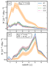 |
Fig. 1. Comparison of the S850 flux densities of the EAGLE galaxies calculated using the RT or the parametric relation given in Equation (1) with the parameter values listed in Table 2. Here, the solid blue color shows the RT results, dotted orange shows the results for the Hayward et al. (2013) relation (H13), dashed green the Lovell et al. (2021) relation (L21), and dash-dotted pink the Cochrane et al. (2023) relation (C23). The shaded regions represent 1σ uncertainties. Panels (a) and (b) show the evolution of the co-moving number density for, respectively submillimeter-bright galaxies (S850 > 1 mJy), and submillimeter-faint star-forming galaxies (S850 < 1 mJy, SFR > 80 M⊙/yr). The L21 and C23 relations exhibit very similar results and are consistent with the RT calculations. However, the H13 relation overestimates the submillimeter flux densities compared to RT. |
In Fig. 1a, we compare the number density of submillimeter-bright galaxies with S850> 1 mJy as a function of redshift. We find that the results from L21 and C23 are comparable to each other and also consistent with the RT calculations. On the other hand, the distribution from the H13 relation overpredicts the number of submillimeter-bright galaxies at all the redshifts reaching about 5 times the number density from the RT calculations at z ≈ 2. Similarly, in Fig. 1b, we compare the number density of galaxies with S850< 1 mJy, but forming stars at a rate greater than 80  . Again, we find good agreement between the results of using the L21 and C23 models as well as their consistency with RT calculations. In contrast, the H13 relation underpredicts submillimeter-faint star-forming galaxies.
A comparison of the parameter values in Table 2 shows that the main difference between the models is the normalization factor. This impacts directly on the number of galaxies exceeding the flux density of S850 > 1 mJy as seen in Fig. 1a. As expected, this also influences the number of submillimeter-faint star-forming galaxies as shown Fig. 1b.
Our tests and findings with the EAGLE simulation show that the S850 predictions using the L21 and C23 relations are remarkably closer to the RT calculation compared to the H13 relation. Since these parametric relations are derived using two independent sets of parameters (SFR and dust mass from simulations, and submillimeter flux from RT calculations), any difference in the predicted flux of a galaxy is indeed the result of the assumptions made during the RT calculations. The L21 and C23 relations predict very similar but lower fluxes than the H13 relation. Three differences in the models that could potentially affect the predicted flux densities are the assumed IMF, the contribution of supermassive black hole emission (or lack thereof), and the stellar spectral library. L21 and C23 assume the Chabrier (2003) IMF and do not consider the contribution of supermassive black holes, whereas H13 assumes the Kroupa (2001) IMF and includes emission from supermassive black holes. Finding the main cause of differences in the predictions of these parametric relations requires a detailed systematic analysis, which is outside the scope of this work.
3.2.2. Testing parametric models on observational data
After testing the parametric relations listed in Table 2 using the EAGLE cosmological simulations, we evaluate their predictions for real observational data. For this purpose, we searched for the archival data of (sub)millimeter galaxies where measured SFRs and dust masses are available. We use data from da Cunha et al. (2015), Dudzevičiūtė et al. (2020), and Hyun et al. (2023). The complete sample comprises 892 submillimeter galaxies: 99 from ALMA at 870 μm in the Extended Chandra Deep Field South (ECDF-S: da Cunha et al. 2015), 707 from ALMA at 870 μm in UKIRT Infrared Deep Sky Survey (UKIDSS) Ultra Deep Survey (UKIDSS-UDS: Dudzevičiūtė et al. 2020), and 86 from JCMT at 850 μm in the JWST Time-Domain Field (JWST-TDF) near the north ecliptic pole (Hyun et al. 2023). All these data use the MAGPHYS galaxy SED-fitting code (da Cunha et al. 2008; Battisti et al. 2019) to estimate SFRs and dust masses. We compiled observational flux densities, SFRs, and dust masses from above mentioned datasets for our analysis. The flux densities at 870 μm are scaled to 850 μm by multiplying by 1.09 assuming the modified black body relation following Equation (6) in Section 4.2.
In Fig. 2, we compare 850 μm flux densities obtained using the parametric relations listed in Table 2 with the observed flux densities at 850 μm. Here, blue boxes, orange circles, and green diamonds show H13, L21, and C23 predictions, respectively. Observed flux densities are shown on the x-axis, and modeled flux densities are shown on the y-axis. The uncertainties in the observed flux densities are obtained from the literature, while the errors in the modeled flux densities represent 16th and 84th percentiles from 10 000 flux density samples per object. These samples are generated by randomly selecting 10 000 values of SFR and dust mass within their observed uncertainty ranges. For the visual clarity of the correspondence, we have also shown the density contours for each relation using respective colors. The black solid line represents one-to-one relation between observed and modeled flux densities. It is clear that the H13 model better represents the observations than the L21 and C23 models for the whole flux density range. The L21 and C23 models underpredict the flux densities for brighter galaxies. This is the first analysis in which we have tested and compared the predictability of these models on observed fluxes.
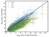 |
Fig. 2. Comparison of observed flux densities with flux densities predicted using the parametric relations listed in Table 2 and observed SFRs and dust masses. The boxes in blue, circles in orange, and diamonds in green respectively represent the H13, L21, and C23 relations. The black solid line is the line of equality for visual guidance. It is clear that H13 reproduces the observed fluxes better than the L21 and C23. (See Section 3.2.2 for more details). |
To conclude our test on observational data, we find that the H13 relation better reproduces observed flux densities for given observed SFRs and dust masses. However, the L21 and C23 underpredict for brighter galaxies. Our analysis shows that the L21 and C23 models predict similar flux densities, but lower than the H13 model. The L21 and C23 models work better for the EAGLE simulation, whereas H13 works better for observations. Hence, for the sake of completeness, we show our results using the L21 and H13 relations unless explicitly stated otherwise.
4. Results
In this section, we discuss our results from the TNG100, TNG300, and FLAMINGO simulations. We particularly focus on the new large-volume FLAMINGO simulations. For clarity, in the main text, we show results for the fiducial FLAMINGO simulation L1_m8, and refer to it as FLAMINGO unless explicitly stated otherwise. The FLAMINGO simulations with different box sizes and resolutions, different galaxy formation prescriptions, and cosmologies are discussed briefly in the appendices (see Appendices B and C). In this section, we present the redshift distributions, source number counts, contribution to SFRD, place on stellar mass−SFR plane, and flux density functions. We also compare our findings with the available observational data.
4.1. Redshift distribution
The redshift distribution of submillimeter galaxies provides relevant information on their assembly and peak activity. In this subsection, we focus on the shape of our predicted distributions. The submillimeter source number counts are discussed in the next subsection. In Fig. 3, we present the redshift distributions of submillimeter-bright galaxies (S850 > 3 mJy) for the FLAMINGO, TNG300, and TNG100 simulations in, respectively, blue, orange, and green colors. The top panel shows predictions using the L21 relation, and the bottom panel displays predictions assuming the H13 relation. The gray colors show the recent observational redshift distribution from Dudzevičiūtė et al. (2020) and Simpson et al. (2020). We have normalized all the distributions by the projected sky area and the redshift bin-sizes. At the bottom of each panel, we indicate the median values of each distribution with their respective colors using small vertical bars.
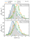 |
Fig. 3. Redshift distribution of submillimeter-bright galaxies with S850 > 3 mJy in the FLAMINGO (blue), TNG300 (orange), and TNG100 (green) simulations. The gray color histograms represent recent observational estimates from Dudzevičiūtė et al. (2020) [Dud+20], and Simpson et al. (2020) [Sim+20]. All the distributions have been re-scaled to match the height of the Dudzevičiūtė et al. (2020) distribution. The small bars at the bottom of each panel indicate the medians of the respective distributions. The top panel shows predictions assuming the L21 relation, while the bottom panel is for the H13 relation. Quantitatively, FLAMINGO better reproduces the observed distribution for the H13 relation (see Section 4.1 for more details). |
For comparison, we rescale all the distributions to match the height of the observed distribution reported in Dudzevičiūtė et al. (2020). This rescaling of the FLAMINGO, TNG300, TNG100 distributions, respectively, requires factors 3.7, 17.8, and 25.5 for the L21 relation and 0.8, 6.8, and 8.7 for the H13 relation. The Simpson et al. (2020) distribution requires a scaling factor of 4.7 to match the height of Dudzevičiūtė et al. (2020). We remind the reader that Dudzevičiūtė et al. (2020) carried out ALMA follow-up of 716 submillimeter galaxies with S850 > 3.6 mJy in a 0.96 deg2 sky area. Their final sample comprises 707 submillimeter galaxies with S870 > 0.6 mJy. On the other hand, Simpson et al. (2020) carried out ALMA follow-up of 183 submillimeter galaxies with S850 > 6.2 mJy in 1.6 deg2 area. Their final sample comprises 182 submillimeter galaxies with S870 > 0.7 mJy. The higher flux density selection threshold employed by Simpson et al. (2020) compared to Dudzevičiūtė et al. (2020) requires scaling their distribution by a factor of 4.7 to align it with the latter.
For the L21 relation, TNG100 and TNG300 show very similar distributions with a small irregularity in TNG100 at z ≈ 3.5 due to its relatively small box size for statistical sampling of bright SMGs. As compared to the observed distributions, both TNG100 and TNG300 peak at higher redshifts. The median redshifts of TNG100 and TNG300 are zmed = 3.28 ± 0.051 and 3.49 ± 0.001, respectively. On the other hand, the FLAMINGO simulation shows remarkable similarity with the shape of observed distributions having median redshift zmed = 2.45 ± 0.001. The median redshift for Dudzevičiūtė et al. (2020) is zmed = 2.61 ± 0.08 and the median redshift for Simpson et al. (2020) is zmed = 2.68 ± 0.06. In addition, the low- and high-redshift tails of the FLAMINGO simulation nicely trace the observed pattern. The small difference seen between the median redshifts of FLAMINGO and the observational data may be due to the effect of sample selection. There is evidence that the redshift distributions for galaxies selected at longer wavelengths and/or brighter flux density tend to peak at higher redshift (e.g., Pope et al. 2005; Brisbin et al. 2017; Lagos et al. 2020; Reuter et al. 2020). We discuss this further later in this section.
The TNG100 and TNG300 redshift distributions are very similar if instead of the L21 we use the H13 relation as shown in the bottom panel of Fig. 3, again with a small irregularity at z ≈ 3.5 in TNG100. However, compared with the predictions using the L21 relation, the predictions using H13 relation move slightly toward lower redshifts. The median redshifts for TNG100 and TNG300 drift to zmed = 2.90 ± 0.048 and 3.28 ± 0.112 respectively. Still, the overall distributions of TNG100 and TNG300 are far from the observed distributions. On the other hand, the median redshift for FLAMINGO changes to 2.35 ± 0.001. Though FLAMINGO shows a small shift toward low-redshift, its predictions are matching the observed distributions quite well.
As pointed out earlier, the median of the redshift distribution moves toward higher redshifts when we select brighter galaxies (Pope et al. 2005; Brisbin et al. 2017) or observe at longer wavelengths (Lagos et al. 2020; Reuter et al. 2020). The statistically representative volume of FLAMINGO (in particular) provides us with the opportunity to compare these observed trends with predicted distributions from parametric relations. To investigate the effect of the flux density cuts on the median values of the redshift distributions, we plot the median of redshifts as a function of the S850 flux density cut in Fig. 4 for FLAMINGO. The solid and dotted blue curves represent, respectively, predictions using the L21 and H13 relations. For comparison, we over-plot the observed data points in gray color compiled from various literature (Chapman et al. 2005; Pope et al. 2005; Wardlow et al. 2011; Casey et al. 2013; da Cunha et al. 2015; Danielson et al. 2017; Miettinen et al. 2017; Cowie et al. 2018; Dudzevičiūtė et al. 2020). For both the relations, there is a clear trend of increasing median redshift as we choose a larger flux density cut for selecting brighter galaxies. However, both trends flatten toward higher flux density cuts. Due to the limited observational data, we cannot verify this flattening. Future surveys with large sky coverage will allow us to test these predictions of the FLAMINGO simulation. Additionally, as seen in Fig. 3, the H13 relation predicts a lower or equal median redshift than the L21 relation at any given flux density cut. Given the range of uncertainties in the observations, both the L21 and H13 relations predict observed median redshift trend quite well.
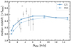 |
Fig. 4. Median of the redshift distributions of submillimeter galaxies as a function of the flux density cut in the FLAMINGO simulation. The solid blue curve represents the prediction using the L21 relation, and the dotted blue curve shows the prediction assuming the H13 relation. Gray color points represent observational estimates obtained from Chapman et al. (2005), Pope et al. (2005), Wardlow et al. (2011), Casey et al. (2013), da Cunha et al. (2015), Danielson et al. (2017), Miettinen et al. (2017), Cowie et al. (2018), Dudzevičiūtė et al. (2020). Both of the models show consistency with the observations and predict a negligible evolution in the median redshift for S850 > 8 mJy. |
4.2. Source number counts
Number counts represent the cumulative number count of (sub)millimeter sources per unit of projected area as a function of flux density. To obtain the source number counts for simulations, we use the method described in Hayward et al. (2013). The cumulative source number counts per unit deg2 at any given flux density Sλ is given by the following expression:
![Mathematical equation: $$ \begin{aligned} \frac{N ({>}S_\lambda )}{\mathrm{[deg^{2}]}} = \left(\frac{\pi }{180}\right)^{2} \int \frac{dN({>}S_\lambda )}{dV}\frac{dV}{d\Omega dz} dz, \end{aligned} $$](/articles/aa/full_html/2025/06/aa53981-25/aa53981-25-eq3.gif) (2)
(2)
where the co-moving volume element per unit solid angle (dΩ) per unit redshift interval (dz) is given as
 (3)
(3)
Here, the co-moving distance to redshift z is
 (4)
(4)
and the redshift-dependent Hubble parameter in a flat universe is
 (5)
(5)
In Equation (2), dN(> Sλ)/dV for any simulation snapshot is computed by diving the total number of sources brighter than Sλ by the co-moving volume of the simulation box. Then we perform a linear interpolation of dN(> Sλ)/dV between the snapshots when evaluating the integral in Equation (2).
In Fig. 5, we show predicted source number counts of submillimeter galaxies in the FLAMINGO (solid blue), TNG300 (dashed orange), TNG100 (dash-dotted green), and EAGLE (dotted pink) simulations. The shaded regions represent the 1σ scatter around the mean for 100 realizations as discussed for EAGLE in Section 3.2.1. The top panel shows the source number counts obtained using the L21 relation, and the bottom panel shows the same for the H13 relation. The gray color open circles and open boxes represent observed source number counts compiled from the literature. For clarity, we have grouped the observed data as JCMT (Casey et al. 2013; Geach et al. 2017; Zavala et al. 2017; Simpson et al. 2019; Shim et al. 2020; Garratt et al. 2023; Hyun et al. 2023; Zeng et al. 2024) and ALMA (Hatsukade et al. 2013; Karim et al. 2013; Simpson et al. 2015, 2020; Fujimoto et al. 2016; Hatsukade et al. 2018; Stach et al. 2018) depending on the observing facility used for these observation. We note that the observed flux density in any (sub)millimeter band SX (or Sλ) is scaled to match the S850 band assuming the following relation used in various publications (e.g., Dunne & Eales 2001; Simpson et al. 2019; Zeng et al. 2024):
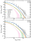 |
Fig. 5. Source number counts of submillimeter galaxies in the FLAMINGO (solid blue), TNG300 (dashed orange), TNG100 (dash-dotted green), and EAGLE (dotted pink) simulations. Shaded regions show 1σ errors for 100 realizations of the modeled submillimeter galaxy population, as discussed in Section 3.2.1. The top panel shows predictions using the L21 relation while the bottom panel uses the H13 relation. For comparison, we have overlaid observed source number counts in gray color, which are grouped as JCMT (Casey et al. 2013; Geach et al. 2017; Zavala et al. 2017; Simpson et al. 2019; Shim et al. 2020; Garratt et al. 2023; Hyun et al. 2023; Zeng et al. 2024) and ALMA (Hatsukade et al. 2013; Karim et al. 2013; Simpson et al. 2015, 2020; Fujimoto et al. 2016; Hatsukade et al. 2018; Stach et al. 2018) according to the observing facility used. We have scaled all the flux densities of ALMA bands to the S850 band assuming a modified black body. The FLAMINGO predicts the observed number counts quite well for the H13 relation. (See Section 4.2 for more detail). |
![Mathematical equation: $$ \begin{aligned} \frac{S_{850}}{S_{X}} = \left(\frac{\nu _{850}}{\nu _{X}}\right)^{\beta } \frac{B(\nu _{850}, T)}{B(\nu _{X}, T)} \approx \left(\frac{\nu _{850}}{\nu _{X}}\right)^{\beta + 2} = \left(\frac{\lambda _{X}\,[{\upmu \mathrm{m}}]}{850}\right)^{\beta + 2}. \end{aligned} $$](/articles/aa/full_html/2025/06/aa53981-25/aa53981-25-eq7.gif) (6)
(6)
This simple flux density conversion relation is the result of (sub)millimeter wavelengths being in the Rayleigh-Jeans region of the Planck function (B(ν, T)). Assuming β = 1.8 (Planck Collaboration XIX 2011), we calculate conversion factors 5.03 for 1.3 mm, 3.71 for 1.2 mm, 2.66 for 1.1 mm, and 1.09 for 870 μm.
None of the simulations reproduce the observed source number counts when using the L21 relation (see the top panel of Fig. 5). At 1 mJy, observational number counts are a factor of ∼100 higher than the EAGLE predictions. Although TNG100 and TNG300 show some improvement as compared to EAGLE, they are far from the observations. Toward the fainter end, the small drop in TNG300 compared to TNG100 is the result of the lower mass resolution of TNG300. There is an excess at bright end in TNG300 as compared to TNG100, showing the importance of a large box size to statistically represent the bright end of number counts. At 1 mJy, the observations are about an order of magnitude higher than the IllustrisTNG predictions. In contrast, FLAMINGO reproduces the observed number counts for S850 < 2 mJy relatively well.
All the source number count distributions shift upward and rightward when using the H13 relation (see the bottom panel of Fig. 5). Although EAGLE, TNG100, and TNG300 show an increase in the source number counts, they remain very discrepant with the observations. On the other hand, FLAMINGO reproduces the observed number counts quite well when using H13 relation. The small excess of observed submillimeter-bright sources relative to FLAMINGO is possibly the effect of multiple source blending as reported in resolved interferometric observations (see, Chen et al. 2013; Hodge et al. 2013; Karim et al. 2013).
Overall, the FLAMINGO simulation simultaneously reproduces the redshift distribution and source number counts of SMGs when using H13 relation. Also, the H13 relation performs better than L21 when applied to observations (see Fig. 2). Hence, it remains valuable for statistical comparison of the observed submillimeter universe with the simulated universe in FLAMINGO when modeled with the H13 relation.
4.3. Contribution to the cosmic SFRD
As (sub)millimeter galaxies are among the most star-forming objects in the universe, we would like to know their contribution to the total cosmic SFRD. To investigate this using FLAMINGO, TNG300, and TNG100 simulations, we plot their submillimeter SFRDs for submillimeter-bright galaxies with S850 > 1 mJy in the left column panels of Fig. 6 using solid blue, dashed orange, and dash-dotted green curves, respectively. Their total SFRDs are shown with dotted curves in respective colors. For comparison, we have also over-plotted the Madau & Dickinson (2014) fit to observations with dotted black color. The shaded regions around the SFRD of submillimeter galaxies represent 1σ scatter for 100 realization as discussed in Section 3.2.1. The top and bottom panels display the predictions for the L21 and H13 relations, respectively. For the total SFRD calculation, we have simply added the SFRs of all the subhalos identified in a given snapshot of the respective simulation. Using the FLAMINGO simulations, we verified that our total SFRD is identical to the SFRD measured on-the-fly using all the gas particles during simulation (as reported in Schaye et al. 2023). The open circles and boxes represent observational estimates for the SFRD of submillimeter galaxies brighter than 1 mJy from Swinbank et al. (2014) and Dudzevičiūtė et al. (2020), respectively. The total SFRD and the ratio of submillimeter to total SFRD of FLAMINGO show a small kink at z ≈ 2. This kink is only visible in the high-resolution model and absent in other FLAMINGO models (see, Figs. A, B, C). Presently, we do not have an explanation for this kink (see, Schaye et al. 2023).
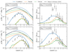 |
Fig. 6. Left column: Contribution of submillimeter galaxies with S850 > 1 mJy to the cosmic SFRD in the FLAMINGO (solid blue), TNG300 (dashed orange), and TNG100 (dash-dotted green) simulations. Dotted curves represent the total SFRD in corresponding colors. The dotted black color show the Madau & Dickinson (2014) fit to observations. The top panel shows predictions using the L21 relation, while the bottom panel using the H13 relation. The shaded regions around SFRD of submillimeter galaxies are 1σ uncertainty for 100 realizations. For comparison, we show submillimeter observations from Swinbank et al. (2014) and Dudzevičiūtė et al. (2020) using, respectively, open circles and boxes. Right column: Ratio of submillimeter to total SFRD corresponding to the left column. We use the Madau & Dickinson (2014) cosmic SFRD to estimate observational ratio. At peak activity, the submillimeter contribution in the FLAMINGO simulation is about 27% for the H13 Model. |
From the left column of Fig. 6 it is clear that FLAMINGO predicts significantly higher contribution of submillimeter-bright galaxies to the cosmic SFRD than TNG100 and TNG300. There is also a significant difference between the peak SFRD of the submillimeter galaxies; FLAMINGO peaks at a lower redshift (z ≈ 2.6) than IllustrisTNG (z ≈ 3.7). A similar shift is also evident for the total cosmic SFRD, which indeed is the reason for the shift in the redshift distribution of IllustrisTNG submillimeter galaxies toward higher redshifts, as seen in Fig. 3. Since the H13 relation predicts higher submillimeter flux densities than the L21 relation, we see a larger contribution of submillimeter galaxies when using the H13 relation as can be perceived from the comparison of the top and bottom panels. Additionally, the observed maximum contribution of submillimeter galaxies to the cosmic SFRD is better reproduced in FLAMINGO simulations when using the H13 relation (see the bottom-right panel in Fig. 6).
From the left panels of Fig. 6, it seems that the contributions of submillimeter galaxies in TNG100 and TNG300 simulations are consistent with each other. However, their total cosmic SFRDs differ significantly. The FLAMINGO simulations were not calibrated to the cosmic SFRD or any other z > 0 galaxy observations (Schaye et al. 2023), yet they show remarkable consistency with observation, particularly for z < 2. On the other hand, the IllustrisTNG simulations were calibrated to the cosmic SFRD for z < 10 (Pillepich et al. 2018), yet they disagree with the observations. For instance, TNG100 is consistent with observation for z > 3, but TNG300 has a lower SFRD in the whole redshift range. Therefore, to quantify the contribution of submillimeter galaxies to the cosmic SFRD, we calculate the ratio of the submillimeter SFRD to the total SFRD as shown in corresponding right column panels of Fig. 6. The maximum submillimeter contribution to cosmic SFRD in the FLAMINGO simulation reaches to ≈15% for the L21 relation and ≈27% for the H13 relation at redshift z = 2.6. However, the highest contribution of submillimeter galaxies to the cosmic SFRD in TNG300 reaches only ≈12% for the L21 relation and ≈18% for the H13 relation at redshift z = 3.7 which is about 2/3 of the FLAMINGO prediction. Further, the maximum submillimeter contribution to the cosmic SFRD in FLAMINGO reasonably matches with observational estimates when using the H13 relation. The TNG100 predicts an even lower contribution than TNG300. This comparison between TNG300 and TNG100 highlights the importance of a large box size for the statistical modeling of the submillimeter galaxy population in cosmological simulations. In Appendix A, we show the effect of box size for the FLAMINGO simulations, and confirm that a 1 Gpc box is large enough to robustly model submillimeter galaxy population.
4.4. Star formation rates and stellar masses
The submillimeter galaxies are characterized by their SFRs and dust mass content. For example, a highly star-forming galaxy with negligible dust content will produce a smaller (sub)millimeter flux than a galaxy with a low SFR but a large dust content. These effects can move SMGs on the SFR and stellar mass plane with the evolution of dust in the Universe. To investigate the evolution of SMGs on the SFR − stellar mass plane, in Fig. 7, we plot the median SFR and stellar mass relation of SMGs in the FLAMINGO simulation from z = 6 to z = 0.5. For a detailed study, we have grouped SMGs into four flux density ranges shown with yellow (1 ≤ S850/mJy < 2), orange (2 ≤ S850/mJy < 3), green (3 ≤ S850/mJy < 5), and pink (S850 > 5 mJy) color curves. The respective shaded regions around the median relations represent the 16–84th percentile range. The gray color maps in the background show the distribution of all the galaxies in FLAMINGO. Here, we have shown the SFRs and stellar masses within a spherical aperture of 30 pkpc radius, which is used for submillimeter flux density calculation in this work. Given the remarkable consistency of the H13 predictions with observations of the SMG population, we only show flux densities obtained from the H13 relation. For comparison, we over-plot observed fitting relations for the SFMS of all galaxies from Popesso et al. (2023) in red color.
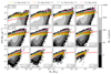 |
Fig. 7. Evolution of the median SFR−stellar mass relation in the FLAMINGO simulation from z = 6 to z = 0.5 for SMGs grouped into four flux density ranges shown with yellow (1 ≤ S850/mJy < 2), orange (2 ≤ S850/mJy < 3), green (3 ≤ S850/mJy < 5), and pink (S850 ≥ 5 mJy) color curves. Their respective shaded regions represent 16–84th percentiles. The background gray color maps show the distribution of all FLAMINGO galaxies. The red color curves display the fit to the observed SFMS of galaxies given in Popesso et al. (2023). Here, we have shown SFRs and stellar masses within spherical apertures of 30 pkpc, and flux densities using H13 model. At all redshifts, SMGs tend to fall on or above the SFMS of galaxies. Most of the z ≤ 1 or z > 6 SMGs are starburst galaxies. |
First, Fig. 7 shows that the FLAMINGO reproduces the SFMS from Popesso et al. (2023), between z = 5.0 − 0.5 with slight deviations at redshifts z > 5. If we now focus on the SMG population, we find that almost all the SMGs brighter than 3 mJy lie above the SFMS throughout the cosmic evolution. This suggests that the bright SMGs are always starburst galaxies On the other hand, majority of SMGs with 1 ≤ S850/mJy < 3 lie on the SFMS in the redshift interval z = 5.0 − 1.5, whereas they lie above SFMS for z ≤ 1 or z > 6, belonging to starburst galaxies. Our z ≤ 1 redshift results are consistent with Michałowski et al. (2017) who reported that all the z < 1 SCUBA2 SMGs above the SFMS. Moreover, the four groups of flux densities in Fig. 7 remain significantly distinct from z = 5.0 to z = 0.5, specifically for massive galaxies (M∗ > 2 × 10¹¹ M⊙). This indicates a strong correlation between (sub)millimeter flux density and SFR. However, this correlation weakens toward low-mass SMGs (M∗ < 2 × 10¹¹ M⊙) and for z > 5.0 SMGs, where we notice significant overlap among the four groups. Additionally, all the SMGs (indeed all galaxies) in FLAMINGO at z > 6.0 have stellar masses < 2 × 10¹¹ M⊙ (for brevity, z > 6.0 redshifts are not shown here).
At a given stellar mass, the median SFRs of the four SMG groups described in Fig. 7 slowly decrease with decreasing redshift. The high-redshift SMGs show higher SFRs than the low redshift SMGs for the same flux density. This is the effect of dust enrichment in the Universe, which counter-balances the flux density reduction due to the evolution of the SFR. Magliocchetti et al. (2013), Wilkinson et al. (2017) report downsizing of halos for a given SFR. From their analysis, they inferred that the host halos of SMGs at lower redshift have a lower mass than those at higher redshift for the same star formation activity. Our analysis does not appear to show such a downsizing effect (also see Lim et al. 2020). We found SMGs with a range of stellar masses for a given SFR, specifically SMGs with 1 ≤ S850/mJy < 3.
4.5. Comparison with previous works
Reproducing the observed properties of SMGs still represents a significant challenge for cosmological simulations. In terms of the number counts of SMGs, SAMs and hydrodynamical simulations have shown difficulties in modeling observational trends4. For instance, Baugh et al. (2005) used a top-heavy IMF and allowed starburst during minor and major mergers in GALFORM SAM to match the SMG number counts. More recent works using SAMs such as Lagos et al. (2019) (see also Safarzadeh et al. 2017) reproduce the faint end of the SMG number counts without invoking top-heavy IMF assumptions while overestimating the number of bright sources.
Likewise, cosmological hydrodynamical simulations tend to underpredict the submillimeter-bright sources. This effect has been attributed to the lack of abundant starbursts, discernible offset from the SFMS, choice of IMF, and small volume of the simulation box. However, numerous studies have shown good concordance with observations. In particular, Shimizu et al. (2012) reproduce the SMG number counts at S850 ∼ 5 − 10 mJy using a box of 100 Mpc/h side length. They assumed a simplified dust model with DTM = 0.5 and calculated the optical depth for UV continuum photons in a sphere. Fardal et al. (2001) modeled the submillimeter fluxes in their simulation using a parametric relation as a function of the temperature of the dust and the emissivity index. They showed a strong dependence of the SMG number counts on the assumed dust temperature and emissivity law. Also, Lovell et al. (2021) using 3D RT calculations on SIMBA galaxies report a good agreement on the shape of the number counts, while normalization is within −0.25 dex at S850 > 3 mJy.
In our study, we use parametric formulations derived from RT calculations from previous investigations (Hayward et al. 2013; Lovell et al. 2021; Cochrane et al. 2023) in hydrodynamical simulations to model the submillimeter flux, maintaining consistency with the RT calculations. Furthermore, we implement large cosmological boxes such as FLAMINGO, which reduce potential box-size effects. Implementing the same parametric formulation in EAGLE, TNG100, TNG300, and FLAMINGO and comparing the results of the number counts suggest that subgrid physics plays an important role in reproducing the observational number counts for SMGs.
The redshift distribution of the SMGs also shows a discrepancy between observations and cosmological simulations. Using 3D RT calculations, McAlpine et al. (2019) selected a sample of SMGs (S850 ≥ 1 mJy) from the EAGLE simulation where photometric fluxes of galaxies are measured. They find that, even when the number counts are underestimated, the median redshift of SMGs is z ≈ 2.5, in good agreement with the observations. Also, Lovell et al. (2021) show good agreement with the redshift distributions. Our results using parametric relations show that only FLAMINGO can reproduce the redshift distribution from observational data, while TNG100 and TNG300 are shifted to higher redshifts. This again indicates that the cosmic evolution of dust mass, star formation, and the role of subgrid physics in simulations can produce different results when modeling the SMG population. Interestingly, here we use the parametric model L21 obtained using SIMBA, which reproduces the number counts and the redshift distribution. When this model is implemented in other simulations, we find no agreement as good as they do. In contrast, H13 provides a better match with observational data.
5. Predictions for flux density functions
In this section, we use the submillimeter galaxies population in FLAMINGO simulation to predict their flux density functions at different redshifts. Fig. 8 shows the flux density functions from redshift z = 0.5 to 6.0 using the L21 model in the top panel and the H13 model in the bottom panel. At all flux densities shown here, the submillimeter population grows monotonically from z = 6.0 to z = 2.5 as is evident in the two panels. The number of brighter sources increases at higher rate than the fainter sources. For example, from redshift z = 6.0 to z = 2.5, the submillimeter population grows by about a factor of ∼10 at 0.1 mJy, and about a factor of ∼60 at 1 mJy. After the that bright submillimeter population depletes rapidly with decreasing redshift. This evolution of submillimeter population changes the shape of flux density function across cosmic time. The low-redshift flux density functions show prominent knee as compare to high-redshift flux density functions. Also, the location of the knee moves toward lower flux density side with decreasing redshift as clearly visible in two panels.
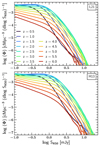 |
Fig. 8. Flux density functions of submillimeter galaxies in the FLAMINGO simulation for z = 0.5 − 6.0 redshift range. The top panel shows prediction using the L21 relation, and the bottom panel displays predictions assuming the H13 relation. The brighter sources increase at a higher rate than the fainter sources from z = 6.0 to z = 2.5, and this is followed by a rapid depletion of bright sources for z < 2.5. |
The increasing submillimeter population from z = 6.0 to z = 2.5 in both the panels is expected, given the dependency of modeled submillimeter flux on the SFR, which is strongly linked with the cosmic SFRD. For a quantitative characterization of this evolution, we fit the Schechter function defined as
 (7)
(7)
where ϕ* is the normalization parameter, S* is the characteristic flux density, and α is the slope parameter.
In Fig. 9, we show the redshift evolution of the Schechter function fitting parameters ϕ* (top panel), S* (middle panel), and α (bottom panel) for the flux density functions. The blue and orange lines with circles correspond to the fitting parameters for the L21 and H13 models, respectively, when the three parameters are left unconstrained. The lines with boxes show results when we arbitrarily fix S* = 1.5 mJy. We constrain the fits in the range of S850 = [0.1 − 25] mJy for the H13 and S850 = [0.1 − 25]/1.75 mJy for the L21 (since the H13 model predicts about a factor of 1.75 higher flux densities than the L21 model on average).
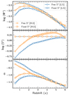 |
Fig. 9. Redshift evolution of the Schechter function fitting parameters for the flux density function shown in Fig. 8. The solid blue and dotted orange curves with circles respectively represent the fitting parameters for the L21 and H13 models. To exhibit the evolution of the flux density functions, we also show the fitting parameters for an arbitrarily fixed value of S* = 1.5 mJy using solid blue and dotted orange curves with boxes for the L21 and H13, respectively. The shaded regions around the curves represent fitting uncertainties. |
Qualitatively, the parameters of the Schechter function demonstrate comparable trends for both the L21 and H13 relations. We find that the normalization parameter ϕ* increases with decreasing redshift when all parameters are free during fitting. However, for a fixed value of S*, the normalization parameter increases until z ≈ 2 and then decreases indicating the growth of the SMG population, as evident from the flux density functions shown in Fig. 8. When we leave the characteristic flux density S* as a free parameter, it changes very slowly between z ≃ 6.0 − 2.5 and then decreases sharply with decreasing redshift for z < 2.5, an indication of the reduction in the submillimeter-bright population. A similar qualitative evolution has been reported for the infrared luminosity functions of galaxies (e.g., Gruppioni et al. 2013; Fujimoto et al. 2024; Traina et al. 2024). We find that the slope parameter α increases linearly with decreasing redshift for free S*, an indication of flattening toward faint-end flux density function as seen in Fig. 8. For a fixed S*, it increases until z = 2.0 and then decreases with decreasing redshift.
6. Predictions for the TolTEC UDS and LSS surveys
The remarkable good agreement between the predictions of the FLAMINGO simulation and observations of (sub)millimeter bright galaxies, particularly using the H13 relation, allows us to make predictions for upcoming observational surveys. In particular, the future TolTEC5 camera (Wilson et al. 2020) at the 50-m Large Millimeter Telescope (Hughes et al. 2020) will provide new insights into dust-obscured star-forming galaxies. Its high mapping speeds and high angular resolution will allow conducting two public legacy surveys at wavelengths of 1.1 mm, 1.4 mm, and 2.0 mm: the 0.8 deg2 UDS and the 40−60 deg2 LSS.
The UDS will reach an optimal depth of σ1.1 ≈ 0.025 mJy at 1.1 mm, σ1.4 ≈ 0.018 mJy at 1.4 mm, and σ2.0 ≈ 0.012 mJy at 2.0 mm, whereas the depth of LSS will be ten times shallower than UDS. Here we use our FLAMINGO submillimeter galaxies catalog to make predictions for the TolTEC UDS and LSS surveys. Although we provide preliminary predictions, we plan to expand our forecasts for the UDS and LSS surveys in a future study. For this analysis, we scale the flux densities at 850 μm to the TolTEC bands using Equation (6).
Fig. 10 shows the predicted redshift distributions, source number counts, SFRD of submillimeter galaxies, and ratio of submillimeter SFRD to cosmic SFRD for the TolTEC UDS survey above the 4σ detection threshold. For brevity, we only show the predictions assuming the H13 relation, as H13 reproduces the 850 μm observations quite well. The blue, orange, and green color curves represent, respectively, 1.1 mm, 1.4 mm, and 2.0 mm predictions. The vertical dashed lines in the top-right panel indicate the 4σ limits of the UDS survey, and the vertical dotted lines indicate the 4σ limits of the LSS survey. The yellow dashed curve in the bottom-left panel shows the total cosmic SFRD in the FLAMINGO simulation, and the black dashed curve represents Madau & Dickinson (2014) fit to the observations.
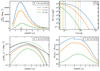 |
Fig. 10. TolTEC UDS survey predictions for redshift distributions (top-left panel), source number counts (top-right panel), SFRDs (bottom-left panel), and ratio of submillimeter SFRDs to the total cosmic SFRDs (bottom-right panel) using the H13 relation and the FLAMINGO simulation. The blue, orange and green curves respectively represent 1.1 mm, 1.4 mm, and 2.0 mm wavelength bands. Vertical dashed and dotted lines in top-right panel indicate the 4σ depths of the TolTEC UDS and LSS surveys, respectively. In the bottom-left panel, the green dotted curve is the total cosmic SFRD and solid curves are (sub)millimeter SFRDs of FLAMINGO, and the black dotted curve is the Madau & Dickinson (2014) fit to observations. The TolTEC 0.8 deg2 UDS survey at 1.1 mm is expected to observe ≈80 000 sources above the 4σ detection limit, which will contribute to about 50% of the cosmic SFRD at z ≈ 2.5. |
From the top-left panel of Fig. 10, we observe that the median values of the redshift distributions in the three TolTEC bands are between z ≈ 1.95 − 2.15. Due to survey depth limits, we expect that the 1.1 mm distribution will have a slightly lower median value than the 2.0 mm distribution because brighter (sub)millimeter galaxies tend to lie at higher redshifts (see Section 4.1). Studies suggest that 2 mm observations preferentially select high-redshift galaxies (Casey et al. 2021). However, our analysis shows only marginal difference between median redshifts of 1.1 mm and 2.0 mm distributions likely because we have modeled them by scaling 850 μm fluxes. The top-right panel of Fig. 10 shows the FLAMINGO predictions that the TolTEC UDS survey will observe about 13 000 galaxies at 2.0 mm, 51 200 galaxies at 1.4 mm, and 80 000 galaxies at 1.1 mm. Similarly, we expect that the TolTEC LSS survey will observe about 60 − 90 galaxies at 2.0 mm, 7500 − 11 300 galaxies at 1.4 mm, 73 000 − 109 400 galaxies at 1.1 mm. The bottom-left panel of Fig. 10 compares (sub)millimeter SFRDs for the three TolTEC bands with the total cosmic SFRD. Thebottom-right panel shows their relative contributions. At z ≈ 2.5, we expect that the TolTEC UDS survey will reveal about 20% of the total SFRD in the 2.0 mm band, 40% SFRD in the 1.4 mm band, and about 50% SFRD in the 1.1 mm band. We note that the contribution of submillimeter galaxies to cosmic SFRD in three bands is not mutually exclusive because all the galaxies observed in longer wavelength band will also be observed in shorter wavelength band. Our predictions can slightly be affected by the cosmic variance and multiple source blending.
7. Conclusions
In this work, we utilize three state-of-the-art cosmological hydrodynamical simulations (EAGLE, IllustrisTNG, and FLAMINGO) to model (sub)millimeter flux densities in galaxies, compare their properties with observations, and make predictions for the upcoming TolTEC surveys. We summarize our main results as follows.
-
We take advantage of the EAGLE RT calculations from Camps et al. (2018) to test the H13 (Hayward et al. 2013), L21 (Lovell et al. 2021), and C23 (Cochrane et al. 2023) parametric models for the SCUBA2_850 flux density measurement using the SFR and dust mass of galaxies. Furthermore, we test the predictions of these models on the observational sample of 892 SMGs compiled from the literature, where SFRs and dust masses are available. As shown in Table 2, the main difference between the parametric models is the normalization factor, which impacts the number of galaxies exceeding the flux density S850> 1 mJy. Our analysis shows that L21 and C23 models exhibit remarkable consistency with the EAGLE RT calculations, whereas the H13 model overestimates the flux densities when compared to the EAGLE RT results (see Fig. 1). In contrast, the H13 model reproduces the observed flux densities much better than L21 and C23, which tend to underpredict them (see Fig. 2). Based on these findings, we choose to continue our study with the H13 and L21 parametric models.
-
We find that the FLAMINGO simulation reproduces the shape and median of the observed redshift distribution of SMGs for H13 and L21 parametric models. On the other hand, the redshift distribution of SMGs in IllustrisTNG peaks at a higher redshift than observed for both parametric models (see Fig. 3). Interestingly, our results show that using the H13 model, the FLAMINGO simulation can reproduce the source number counts of SMGs from observations (see Fig. 5). This is not the case for the IllustrisTNG and EAGLE simulations, which underpredict the trend.
-
We find that the contribution of submillimeter-bright galaxies (S850 > 1 mJy) to the cosmic SFRD reaches about 27% at z = 2.6 in the FLAMINGO simulation. This finding is consistent with observational estimates (see, Swinbank et al. 2014; Dudzevičiūtė et al. 2020, and our Fig. 6).
-
All the SMGs with S850 > 3 mJy are starburst galaxies, and they lie above the SFMS of galaxies throughout cosmic evolution. The SMGs with 1 ≤ S850/mJy < 3 fall at the SFMS in the redshift interval z = 5.0 − 1.5 and above it for z ≤ 1 or z ≥ 6.0 (see Fig. 7). At all redshifts, the flux densities of high-mass SMGs (M∗ > 2 × 10¹¹ M⊙) show a strong correlation with their SFRs, while this correlation weakens for low-mass SMGs. In contrast to Magliocchetti et al. (2013), Wilkinson et al. (2017), for the same SFR, we do not find a downsizing effect in the FLAMINGO SMGs.
-
We use FLAMINGO to make predictions for the flux density function with redshift. Our results reveal a rise in SMG abundance from z = 6 to z = 2.5 (see Fig. 8). The Schechter function fits to the flux density functions for a fixed characteristic flux density (S*) show a linearly increasing slope parameter (α) from z = 6 to z = 2.5 and then decreasing. Between z = 2.5 − 0, we find that the depletion of SMGs accelerates with increasing flux density, indicating rapid fading of the brightest submillimeter phase (see Fig. 9).
-
We provide predictions for the upcoming TolTEC 0.8 deg2 UDS and 40−60 deg2 LSS surveys at the 4σ detection threshold. Our results suggest that the UDS survey will observe about 13 000 galaxies at 2.0 mm; 51 200 galaxies at 1.4 mm; and 80 000 galaxies at 1.1 mm. The UDS survey will observe a large fraction of low-mass SMGs. About 13 000 bright galaxies will be observed in three bands, thus providing a large sample for studying dust properties. On the other hand, the LSS survey will observe about 60 − 90 galaxies at 2.0 mm; 7500 − 11 300 galaxies at 1.4 mm; and 73 000 − 109 400 galaxies at 1.1 mm. Furthermore, the UDS survey will reveal (sub)millimeter galaxies that contribute about 50% to the cosmic SFRD at z ≈ 2.5 in 1.1 mm band (see Fig. 10).
This is the first study to reproduce the observed properties of submillimeter galaxies using the fully hydrodynamical cosmological simulation FLAMINGO, without invoking a top-heavy IMF. The SMG population we have modeled represents an observationally representative sample of SMGs. Therefore, it has several implications for upcoming submillimeter surveys and ongoing JWST observations of submillimeter galaxies. Further studies of SMGs in FLAMINGO complementing recent observations will provide deeper insights into their formation and evolution at high redshift.
An extensive comparison of previous works can be found in Lovell et al. 2021 (see their Figure 10).
Acknowledgments
We thank the anonymous reviewer for constructive suggestions on the manuscript. AK and MCA acknowledge support from ALMA fund with code 31220021 and from ANID BASAL project FB210003. ADMD thanks Fondecyt for financial support through the Fondecyt Regular 2021 grant 1210612. We thank CC Hayward, SM Stach, E van Kampen, P Camps, M Baes, R Cochrane, and I Smail for their comments and suggestions. HSH acknowledges the support of the National Research Foundation of Korea (NRF) grant funded by the Korea government (MSIT), NRF-2021R1A2C1094577, Samsung Electronic Co., Ltd. (Project Number IO220811-01945-01), and Hyunsong Educational & Cultural Foundation. J.L. is supported by the National Research Foundation of Korea (NRF-2021R1C1C2011626). We make use of Matplotlib (Hunter 2007), Numpy (Harris et al. 2020), Pandas (Wes McKinney 2010; The pandas development team 2020), Scipy (Virtanen et al. 2020), WebPlotDigitizer in this work. This work used the RAGNAR computing facility available at Universidad Andrés Bello. This work used the DiRAC@Durham facility managed by the Institute for Computational Cosmology on behalf of the STFC DiRAC HPC Facility (www.dirac.ac.uk). The equipment was funded by BEIS capital funding via STFC capital grants ST/P002293/1, ST/R002371/1 and ST/S002502/1, Durham University and STFC operations grant ST/R000832/1. DiRAC is part of the National e-Infrastructure. We acknowledge the Virgo Consortium for making their simulation data available. The EAGLE simulations were performed using the DiRAC-2 facility at Durham, managed by the ICC, and the PRACE facility Curie based in France at TGCC, CEA, Bruyères-le-Châtel. The IllustrisTNG simulations were undertaken with compute time awarded by the Gauss Centre for Supercomputing (GCS) under GCS Large-Scale Projects GCS-ILLU and GCS-DWAR on the GCS share of the supercomputer Hazel Hen at the High Performance Computing Center Stuttgart (HLRS), as well as on the machines of the Max Planck Computing and Data Facility (MPCDF) in Garching, Germany.
References
- Abbott, T. M. C., Aguena, M., Alarcon, A., et al. 2022, Phys. Rev. D, 105, 023520 [CrossRef] [Google Scholar]
- Amon, A., Robertson, N. C., Miyatake, H., et al. 2023, MNRAS, 518, 477 [Google Scholar]
- Andrews, M., Artale, M. C., Kumar, A., et al. 2025, A&A, in press, https://doi.org/10.1051/0004-6361/202452628 [Google Scholar]
- Araya-Araya, P., Cochrane, R. K., Hayward, C. C., et al. 2024, ApJ, 977, 204 [Google Scholar]
- Barger, A. J., Cowie, L. L., Sanders, D. B., et al. 1998, Nature, 394, 248 [Google Scholar]
- Barger, A. J., Wang, W. H., Cowie, L. L., et al. 2012, ApJ, 761, 89 [Google Scholar]
- Battisti, A. J., da Cunha, E., Grasha, K., et al. 2019, ApJ, 882, 61 [NASA ADS] [CrossRef] [Google Scholar]
- Baugh, C. M., Lacey, C. G., Frenk, C. S., et al. 2005, MNRAS, 356, 1191 [Google Scholar]
- Blain, A. W. 1997, MNRAS, 290, 553 [NASA ADS] [Google Scholar]
- Blain, A. W., Chapman, S. C., Smail, I., & Ivison, R. 2004, ApJ, 611, 725 [NASA ADS] [CrossRef] [Google Scholar]
- Bothwell, M. S., Smail, I., Chapman, S. C., et al. 2013, MNRAS, 429, 3047 [Google Scholar]
- Brisbin, D., Miettinen, O., Aravena, M., et al. 2017, A&A, 608, A15 [NASA ADS] [CrossRef] [EDP Sciences] [Google Scholar]
- Bruzual, G., & Charlot, S. 2003, MNRAS, 344, 1000 [NASA ADS] [CrossRef] [Google Scholar]
- Camps, P., & Baes, M. 2015, Astron. Comput., 9, 20 [Google Scholar]
- Camps, P., Trčka, A., Trayford, J., et al. 2018, ApJS, 234, 20 [NASA ADS] [CrossRef] [Google Scholar]
- Casey, C. M., Chen, C.-C., Cowie, L. L., et al. 2013, MNRAS, 436, 1919 [NASA ADS] [CrossRef] [Google Scholar]
- Casey, C. M., Narayanan, D., & Cooray, A. 2014, Phys. Rep., 541, 45 [Google Scholar]
- Casey, C. M., Zavala, J. A., Manning, S. M., et al. 2021, ApJ, 923, 215 [NASA ADS] [CrossRef] [Google Scholar]
- Chabrier, G. 2003, PASP, 115, 763 [Google Scholar]
- Chakrabarti, S., Fenner, Y., Cox, T. J., Hernquist, L., & Whitney, B. A. 2008, ApJ, 688, 972 [Google Scholar]
- Chapman, S. C., Blain, A. W., Ivison, R. J., & Smail, I. R. 2003, Nature, 422, 695 [NASA ADS] [CrossRef] [Google Scholar]
- Chapman, S. C., Blain, A. W., Smail, I., & Ivison, R. J. 2005, ApJ, 622, 772 [NASA ADS] [CrossRef] [Google Scholar]
- Chen, C.-C., Cowie, L. L., Barger, A. J., et al. 2013, ApJ, 776, 131 [Google Scholar]
- Chen, C.-C., Smail, I., Swinbank, A. M., et al. 2016, ApJ, 831, 91 [NASA ADS] [CrossRef] [Google Scholar]
- Cochrane, R. K., Hayward, C. C., Anglés-Alcázar, D., & Somerville, R. S. 2023, MNRAS, 518, 5522 [Google Scholar]
- Coppin, K., Chapin, E. L., Mortier, A. M. J., et al. 2006, MNRAS, 372, 1621 [Google Scholar]
- Cowie, L. L., González-López, J., Barger, A. J., et al. 2018, ApJ, 865, 106 [NASA ADS] [CrossRef] [Google Scholar]
- Crain, R. A., Schaye, J., Bower, R. G., et al. 2015, MNRAS, 450, 1937 [NASA ADS] [CrossRef] [Google Scholar]
- da Cunha, E., Charlot, S., & Elbaz, D. 2008, MNRAS, 388, 1595 [Google Scholar]
- da Cunha, E., Walter, F., Smail, I. R., et al. 2015, ApJ, 806, 110 [Google Scholar]
- Danielson, A. L. R., Swinbank, A. M., Smail, I., et al. 2017, ApJ, 840, 78 [NASA ADS] [CrossRef] [Google Scholar]
- Davé, R., Finlator, K., Oppenheimer, B. D., et al. 2010, MNRAS, 404, 1355 [NASA ADS] [Google Scholar]
- Davé, R., Anglés-Alcázar, D., Narayanan, D., et al. 2019, MNRAS, 486, 2827 [Google Scholar]
- Davis, M., Efstathiou, G., Frenk, C. S., & White, S. D. M. 1985, ApJ, 292, 371 [Google Scholar]
- Draine, B. T., & Salpeter, E. E. 1979, ApJ, 231, 77 [NASA ADS] [CrossRef] [Google Scholar]
- Dudzevičiūtė, U., Smail, I., Swinbank, A. M., et al. 2020, MNRAS, 494, 3828 [Google Scholar]
- Dunlop, J. S., McLure, R. J., Biggs, A. D., et al. 2017, MNRAS, 466, 861 [Google Scholar]
- Dunne, L., & Eales, S. A. 2001, MNRAS, 327, 697 [Google Scholar]
- Dwek, E. 1998, ApJ, 501, 643 [NASA ADS] [CrossRef] [Google Scholar]
- Elahi, P. J., Cañas, R., Poulton, R. J. J., et al. 2019, PASA, 36, e021 [NASA ADS] [CrossRef] [Google Scholar]
- Fardal, M. A., Katz, N., Weinberg, D. H., Davé, R., & Hernquist, L. 2001, arXiv e-prints [arXiv:astro-ph/0107290] [Google Scholar]
- Fujimoto, S., Ouchi, M., Ono, Y., et al. 2016, ApJS, 222, 1 [Google Scholar]
- Fujimoto, S., Kohno, K., Ouchi, M., et al. 2024, ApJS, 275, 36 [NASA ADS] [Google Scholar]
- Garratt, T. K., Geach, J. E., Tamura, Y., et al. 2023, MNRAS, 520, 3669 [Google Scholar]
- Geach, J. E., Dunlop, J. S., Halpern, M., et al. 2017, MNRAS, 465, 1789 [Google Scholar]
- Gómez-Guijarro, C., Toft, S., Karim, A., et al. 2018, ApJ, 856, 121 [Google Scholar]
- Greve, T. R., Bertoldi, F., Smail, I., et al. 2005, MNRAS, 359, 1165 [NASA ADS] [CrossRef] [Google Scholar]
- Gruppioni, C., Pozzi, F., Rodighiero, G., et al. 2013, MNRAS, 432, 23 [Google Scholar]
- Harris, C. R., Millman, K. J., van der Walt, S. J., et al. 2020, Nature, 585, 357 [NASA ADS] [CrossRef] [Google Scholar]
- Hatsukade, B., Kohno, K., Aretxaga, I., et al. 2011, MNRAS, 411, 102 [NASA ADS] [CrossRef] [Google Scholar]
- Hatsukade, B., Ohta, K., Seko, A., Yabe, K., & Akiyama, M. 2013, ApJ, 769, L27 [NASA ADS] [CrossRef] [Google Scholar]
- Hatsukade, B., Kohno, K., Yamaguchi, Y., et al. 2018, PASJ, 70, 105 [Google Scholar]
- Hayward, C. C., Kereš, D., Jonsson, P., et al. 2011, ApJ, 743, 159 [CrossRef] [Google Scholar]
- Hayward, C. C., Jonsson, P., Kereš, D., et al. 2012, MNRAS, 424, 951 [Google Scholar]
- Hayward, C. C., Narayanan, D., Kereš, D., et al. 2013, MNRAS, 428, 2529 [Google Scholar]
- Hayward, C. C., Sparre, M., Chapman, S. C., et al. 2021, MNRAS, 502, 2922 [Google Scholar]
- Hezaveh, Y. D., Marrone, D. P., Fassnacht, C. D., et al. 2013, ApJ, 767, 132 [NASA ADS] [CrossRef] [Google Scholar]
- Hickox, R. C., Wardlow, J. L., Smail, I., et al. 2012, MNRAS, 421, 284 [NASA ADS] [Google Scholar]
- Hodge, J. A., Carilli, C. L., Walter, F., et al. 2012, ApJ, 760, 11 [Google Scholar]
- Hodge, J. A., Karim, A., Smail, I., et al. 2013, ApJ, 768, 91 [Google Scholar]
- Hodge, J. A., Smail, I., Walter, F., et al. 2019, ApJ, 876, 130 [Google Scholar]
- Hopkins, P. F., Richards, G. T., & Hernquist, L. 2007, ApJ, 654, 731 [Google Scholar]
- Hopkins, P. F., Wetzel, A., Kereš, D., et al. 2018, MNRAS, 480, 800 [NASA ADS] [CrossRef] [Google Scholar]
- Hughes, D. H., Serjeant, S., Dunlop, J., et al. 1998, Nature, 394, 241 [Google Scholar]
- Hughes, D. H., Schloerb, F. P., Aretxaga, I., et al. 2020, in Ground-based and Airborne Telescopes VIII, eds. H. K. Marshall, J. Spyromilio, & T. Usuda, SPIE Conf. Ser., 11445, 1144522 [Google Scholar]
- Hunter, J. D. 2007, Comput. Sci. Eng., 9, 90 [NASA ADS] [CrossRef] [Google Scholar]
- Hyun, M., Im, M., Smail, I. R., et al. 2023, ApJS, 264, 19 [NASA ADS] [CrossRef] [Google Scholar]
- James, A., Dunne, L., Eales, S., & Edmunds, M. G. 2002, MNRAS, 335, 753 [CrossRef] [Google Scholar]
- Jonsson, P., Groves, B. A., & Cox, T. J. 2010, MNRAS, 403, 17 [NASA ADS] [CrossRef] [Google Scholar]
- Karim, A., Swinbank, A. M., Hodge, J. A., et al. 2013, MNRAS, 432, 2 [Google Scholar]
- Kroupa, P. 2001, MNRAS, 322, 231 [NASA ADS] [CrossRef] [Google Scholar]
- Kugel, R., Schaye, J., Schaller, M., et al. 2023, MNRAS, 526, 6103 [NASA ADS] [CrossRef] [Google Scholar]
- Lagos, C. d. P., Robotham, A. S. G., Trayford, J. W., et al. 2019, MNRAS, 489, 4196 [NASA ADS] [CrossRef] [Google Scholar]
- Lagos, C. d. P., da Cunha, E., Robotham, A. S. G., et al. 2020, MNRAS, 499, 1948 [CrossRef] [Google Scholar]
- Lee, K.-S., Gawiser, E., Park, C., et al. 2024, ApJ, 962, 36 [Google Scholar]
- Leitherer, C., Schaerer, D., Goldader, J. D., et al. 1999, ApJS, 123, 3 [Google Scholar]
- Li, Q., Narayanan, D., & Davé, R. 2019, MNRAS, 490, 1425 [CrossRef] [Google Scholar]
- Lim, C.-F., Chen, C.-C., Smail, I., et al. 2020, ApJ, 895, 104 [NASA ADS] [CrossRef] [Google Scholar]
- Lovell, C. C., Geach, J. E., Davé, R., Narayanan, D., & Li, Q. 2021, MNRAS, 502, 772 [NASA ADS] [CrossRef] [Google Scholar]
- Lovell, C. C., Geach, J. E., Davé, R., et al. 2022, MNRAS, 515, 3644 [CrossRef] [Google Scholar]
- Madau, P., & Dickinson, M. 2014, ARA&A, 52, 415 [Google Scholar]
- Magliocchetti, M., Popesso, P., Rosario, D., et al. 2013, MNRAS, 433, 127 [NASA ADS] [CrossRef] [Google Scholar]
- McAlpine, S., Helly, J. C., Schaller, M., et al. 2016, Astron. Comput., 15, 72 [NASA ADS] [CrossRef] [Google Scholar]
- McAlpine, S., Smail, I., Bower, R. G., et al. 2019, MNRAS, 488, 2440 [NASA ADS] [CrossRef] [Google Scholar]
- McKinney, W. 2010, in Proceedings of the 9th Python in Science Conference, eds. S. van der Walt, & J. Millman, 56 [Google Scholar]
- McKinnon, R., Torrey, P., & Vogelsberger, M. 2016, MNRAS, 457, 3775 [CrossRef] [Google Scholar]
- Michałowski, M. J., Dunlop, J. S., Koprowski, M. P., et al. 2017, MNRAS, 469, 492 [Google Scholar]
- Miettinen, O., Delvecchio, I., Smolčić, V., et al. 2017, A&A, 606, A17 [NASA ADS] [CrossRef] [EDP Sciences] [Google Scholar]
- Muñoz Arancibia, A. M., Navarrete, F. P., Padilla, N. D., et al. 2015, MNRAS, 446, 2291 [CrossRef] [Google Scholar]
- Nandi, S., Das, M., & Dwarakanath, K. S. 2021, MNRAS, 503, 5746 [NASA ADS] [CrossRef] [Google Scholar]
- Narayanan, D., Cox, T. J., Hayward, C. C., Younger, J. D., & Hernquist, L. 2009, MNRAS, 400, 1919 [Google Scholar]
- Narayanan, D., Hayward, C. C., Cox, T. J., et al. 2010, MNRAS, 401, 1613 [Google Scholar]
- Narayanan, D., Turk, M. J., Robitaille, T., et al. 2021, ApJS, 252, 12 [NASA ADS] [CrossRef] [Google Scholar]
- Nava-Moreno, N. A., Montaña, A., Aretxaga, I., et al. 2024, MNRAS, 531, 4900 [Google Scholar]
- Nelson, D., Springel, V., Pillepich, A., et al. 2019, Comput. Astrophys. Cosmol., 6, 2 [Google Scholar]
- Pillepich, A., Springel, V., Nelson, D., et al. 2018, MNRAS, 473, 4077 [Google Scholar]
- Planck Collaboration VI. 2020, A&A, 641, A6 [NASA ADS] [CrossRef] [EDP Sciences] [Google Scholar]
- Planck Collaboration XIX. 2011, A&A, 536, A19 [NASA ADS] [CrossRef] [EDP Sciences] [Google Scholar]
- Ploeckinger, S., & Schaye, J. 2020, MNRAS, 497, 4857 [CrossRef] [Google Scholar]
- Pope, A., Borys, C., Scott, D., et al. 2005, MNRAS, 358, 149 [NASA ADS] [CrossRef] [Google Scholar]
- Popesso, P., Concas, A., Cresci, G., et al. 2023, MNRAS, 519, 1526 [Google Scholar]
- Popping, G., Somerville, R. S., & Galametz, M. 2017, MNRAS, 471, 3152 [NASA ADS] [CrossRef] [Google Scholar]
- Press, W. H., & Davis, M. 1982, ApJ, 259, 449 [Google Scholar]
- Reuter, C., Vieira, J. D., Spilker, J. S., et al. 2020, ApJ, 902, 78 [NASA ADS] [CrossRef] [Google Scholar]
- Rodriguez-Gomez, V., Genel, S., Vogelsberger, M., et al. 2015, MNRAS, 449, 49 [Google Scholar]
- Safarzadeh, M., Lu, Y., & Hayward, C. C. 2017, MNRAS, 472, 2462 [NASA ADS] [CrossRef] [Google Scholar]
- Sánchez-Blázquez, P., Peletier, R. F., Jiménez-Vicente, J., et al. 2006, MNRAS, 371, 703 [Google Scholar]
- Schaller, M., Borrow, J., Draper, P. W., et al. 2024, MNRAS, 530, 2378 [NASA ADS] [CrossRef] [Google Scholar]
- Schaye, J., Dalla Vecchia, C., Booth, C. M., et al. 2010, MNRAS, 402, 1536 [Google Scholar]
- Schaye, J., Crain, R. A., Bower, R. G., et al. 2015, MNRAS, 446, 521 [Google Scholar]
- Schaye, J., Kugel, R., Schaller, M., et al. 2023, MNRAS, 526, 4978 [NASA ADS] [CrossRef] [Google Scholar]
- Scott, K. S., Austermann, J. E., Perera, T. A., et al. 2008, MNRAS, 385, 2225 [NASA ADS] [CrossRef] [Google Scholar]
- Shim, H., Kim, Y., Lee, D., et al. 2020, MNRAS, 498, 5065 [NASA ADS] [CrossRef] [Google Scholar]
- Shimizu, I., Yoshida, N., & Okamoto, T. 2012, MNRAS, 427, 2866 [Google Scholar]
- Simpson, J. M., Swinbank, A. M., Smail, I., et al. 2014, ApJ, 788, 125 [Google Scholar]
- Simpson, J. M., Smail, I., Swinbank, A. M., et al. 2015, ApJ, 807, 128 [Google Scholar]
- Simpson, J. M., Smail, I., Swinbank, A. M., et al. 2019, ApJ, 880, 43 [NASA ADS] [CrossRef] [Google Scholar]
- Simpson, J. M., Smail, I., Dudzevičiūtė, U., et al. 2020, MNRAS, 495, 3409 [Google Scholar]
- Siringo, G., Kreysa, E., Kovács, A., et al. 2009, A&A, 497, 945 [NASA ADS] [CrossRef] [EDP Sciences] [Google Scholar]
- Smail, I., Ivison, R. J., & Blain, A. W. 1997, ApJ, 490, L5 [NASA ADS] [CrossRef] [Google Scholar]
- Smith, D. J. B., Hayward, C. C., Jarvis, M. J., & Simpson, C. 2017, MNRAS, 471, 2453 [Google Scholar]
- Somerville, R. S., Gilmore, R. C., Primack, J. R., & Domínguez, A. 2012, MNRAS, 423, 1992 [NASA ADS] [CrossRef] [Google Scholar]
- Springel, V. 2005, MNRAS, 364, 1105 [Google Scholar]
- Springel, V. 2010, MNRAS, 401, 791 [Google Scholar]
- Springel, V., White, S. D. M., Tormen, G., & Kauffmann, G. 2001, MNRAS, 328, 726 [Google Scholar]
- Springel, V., White, S. D. M., Jenkins, A., et al. 2005, Nature, 435, 629 [Google Scholar]
- Stach, S. M., Smail, I., Swinbank, A. M., et al. 2018, ApJ, 860, 161 [Google Scholar]
- Swinbank, A. M., Simpson, J. M., Smail, I., et al. 2014, MNRAS, 438, 1267 [Google Scholar]
- Tacconi, L. J., Genzel, R., Smail, I., et al. 2008, ApJ, 680, 246 [Google Scholar]
- The pandas development team 2020, https://doi.org/10.5281/zenodo.3509134 [Google Scholar]
- Toft, S., Smolčić, V., Magnelli, B., et al. 2014, ApJ, 782, 68 [Google Scholar]
- Traina, A., Gruppioni, C., Delvecchio, I., et al. 2024, A&A, 681, A118 [NASA ADS] [CrossRef] [EDP Sciences] [Google Scholar]
- Valentino, F., Tanaka, M., Davidzon, I., et al. 2020, ApJ, 889, 93 [Google Scholar]
- Virtanen, P., Gommers, R., Oliphant, T. E., et al. 2020, Nat. Methods, 17, 261 [Google Scholar]
- Wardlow, J. L., Smail, I., Coppin, K. E. K., et al. 2011, MNRAS, 415, 1479 [Google Scholar]
- Weinberger, R., Springel, V., Hernquist, L., et al. 2017, MNRAS, 465, 3291 [Google Scholar]
- Weiß, A., Kovács, A., Coppin, K., et al. 2009, ApJ, 707, 1201 [Google Scholar]
- Wilkinson, A., Almaini, O., Chen, C.-C., et al. 2017, MNRAS, 464, 1380 [NASA ADS] [CrossRef] [Google Scholar]
- Wilson, G. W., Abi-Saad, S., Ade, P., et al. 2020, in Millimeter, Submillimeter, and Far-Infrared Detectors and Instrumentation for Astronomy X, eds. J. Zmuidzinas, & J.-R. Gao, SPIE Conf. Ser., 11453, 1145302 [Google Scholar]
- Yang, C., Omont, A., Beelen, A., et al. 2017, A&A, 608, A144 [NASA ADS] [CrossRef] [EDP Sciences] [Google Scholar]
- Zavala, J. A., Aretxaga, I., Geach, J. E., et al. 2017, MNRAS, 464, 3369 [NASA ADS] [CrossRef] [Google Scholar]
- Zeng, X., Ao, Y., & Zhang, Y. 2024, MNRAS, 528, 2964 [NASA ADS] [CrossRef] [Google Scholar]
- Zhang, Y., Zheng, X. Z., Shi, D. D., et al. 2022, MNRAS, 512, 4893 [NASA ADS] [CrossRef] [Google Scholar]
Appendix A: The effect of box size
This work particularly focuses on one of the FLAMINGO flagship simulations in a box with side length 1 cGpc (L1_m8). In this appendix, we investigate the effect of box size on our findings. For this purpose, we utilize two other FLAMINGO simulations: one in the same box size of 1 cGpc (L1_m9), and another in a larger box size of 2.8 cGpc (L2p8_m9). Both of these simulations have the same mass resolution, but have 8 times lower mass-resolution than the L1_m8 simulation. In Fig. A.1, we compare the redshift distributions, source number counts, SFRDs, and ratio of submillimeter-bright SFRDs to their cosmic SFRDs assuming the H13 model. Simulations L1_m8, L1_m9, and L2p8_m9 are respectively shown with blue, orange, and green colors. To visualize the importance of resolution on the source number counts toward the fainter end, we have over-plotted the observational data.
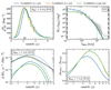 |
Fig. A.1. Comparison of the redshift distributions, source number counts, SFRDs, and ratio of submillimeter-bright SFRDs to cosmic SFRDs using the H13 relation for the three fiducial FLAMINGO simulations with different resolutions and box sizes. Simulations L1_m8, L1_m9, and L2p8_m9 are respectively shown with blue, orange, and green colors. The gray symbols in the top-right panel are observational data. The small bars at the bottom of top-left panel indicate the medians of the respective distributions. In the bottom-left panel, dotted curves are the cosmic SFRDs, solid curves are submillimeter-bright SFRDs, and the black dotted curve is the Madau & Dickinson (2014) fit to observations. The remarkable overlap between L1_m9 and L2p8_m9 shows that a 1 cGpc box side length is large enough for modeling the (sub)millimeter galaxy population. The top-right panel shows that higher resolution improves fainter end source number counts. |
All the panels of Fig. A.1 show remarkable consistency with increasing box size (the orange and green color curves are barely distinguishable). This confirms that the 1 cGpc side length box is sufficiently large to model the (sub)millimeter galaxy population in cosmological simulations. Further, increasing the resolution improves the source number counts toward the faint end while having only a marginal effect on the bright end, as is evident from the blue and orange curves in top-right panel. There is some effect of resolution on the submillimeter SRFD and cosmic SFRD and thus also on the redshift distribution. This is a consequence of the self-consistent evolution of FLAMINGO simulations which were not calibrated to the cosmic SFRD. The simulation with increased resolution (L1_m8) shows a higher cosmic SFRD for z > 2. However, this increase in the cosmic SFRD does not significantly increase the number of submillimeter-bright galaxies, as is evident from the redshift distribution in the top-left panel. This effect results in reducing the contribution of submillimeter galaxies to the cosmic SRFD compared to the other FLAMINGO simulations.
Appendix B: The effect of the galaxy formation prescription
To account for the systematic uncertainties in the observed stellar mass and cluster gas fractions, FLAMINGO includes eight variations of the galaxy formation prescriptions. These simulations with varying galaxy formation prescriptions are performed in a 1 cGpc box (for details see Schaye et al. 2023). In this appendix, we make use of these simulations to test the effect of the galaxy formation prescription on the submillimeter galaxy population. Fig B.1 shows the comparison of redshift distributions, source number counts, SFRDs, and ratio of submillimeter SFRDs to cosmic SFRDs assuming the H13 relation for the simulations with varying galaxy formation prescriptions. In Table B.1, we list the names of the simulations and calibration parameters which they are calibrated for. The AGN feedback particularly affects the cluster gas fraction, and SN feedback particularly affects galaxy stellar mass.
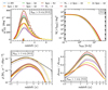 |
Fig. B.1. Same as in Fig. A.1 but comparing FLAMINGO simulations using different galaxy formation prescriptions. Galaxy formation prescription with strongest AGN predicts excess submillimeter-bright sources contributing higher to the cosmic SFRD than other galaxy formation prescriptions. |
Name of the simulations with varying galaxy formation prescriptions and the observed parameters used for calibration.
The top-left panel of Fig B.1 shows that the simulation with the lowest cluster gas fractions, which are mainly controlled by the AGN feedback, predicts the highest number of submillimeter sources brighter than 3 mJy. The low galaxy mass function models predict lower numbers of submillimeter-bright sources. Additionally, the cosmic SFRDs of low galaxy mass function models are lower, as is evident from the bottom-left panel. The ratio of submillimeter-bright SFRDs to cosmic SFRDs in the bottom-right panel clearly indicates that for the models using jet-like AGN feedback, submillimeter galaxies contribute the least to the cosmic SRFD. The predictions of low galaxy mass function models fall in between those of the low gas fraction models. On the other hand, the source number counts in top-right panel are marginally affected by the choice of galaxy formation prescription.
Appendix C: The effect of cosmology
Along with the fiducial cosmology, the four variations of cosmology in the FLAMINGO suite of simulations provide us with the opportunity to test the effect of cosmological parameters on the predicted submillimeter galaxies. Similar to the variations of galaxy formation prescriptions, the variations of cosmologies are also simulated in 1 cGpc boxes. Fig. C.1 illustrates the effect of variation in cosmology on the redshift distributions, source number counts, SFRDs, and ratio of submillimeter SFRDs to cosmic SFRDs assuming the H13 relation. For the cosmological parameters, we refer the reader to Table 4 in Schaye et al. (2023). Briefly, the Dark Energy Survey parameters (Abbott et al. 2022) are Fiducial cosmology (D3A), Planck collaboration parameters (Planck Collaboration VI 2020) with the minimum allowed neutrino mass are Planck cosmology, adjusted Planck collaboration parameters with the maximum allowed neutrino mass are PlanckNu0p24Var cosmology, fixed Planck collaboration parameters with the maximum allowed neutrino mass are PlanckNu0p24Fix cosmology, and Lensing cosmology parameters (Amon et al. 2023) are LS8 cosmology.
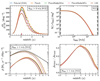 |
Fig. C.1. Same as in Fig. A.1 but comparing FLAMINGO simulations assuming different cosmological parameters. Predictions for all the cosmologies are quite consistent given their cosmic SFRDs. |
All the panels of Fig. C.1 display consistent predictions at low redshift, irrespective of the cosmology. Furthermore, the D3A and Planck cosmologies show similar predictions at all redshifts. The other cosmologies, which have lower values of σ8, predict reduced numbers of submillimeter-bright galaxies toward higher redshift, which is consistent with their relatively lower cosmic SFRDs. The ratio of the submillimeter-bright SFRD to cosmic SFRD in the bottom-right panel exhibits very similar contributions of submillimeter-bright galaxies to the cosmic SFRD for all the cosmologies.
All Tables
Cosmological parameters of different simulations and constraints on data used in this work.
Name of the simulations with varying galaxy formation prescriptions and the observed parameters used for calibration.
All Figures
|
Fig. 1. Comparison of the S850 flux densities of the EAGLE galaxies calculated using the RT or the parametric relation given in Equation (1) with the parameter values listed in Table 2. Here, the solid blue color shows the RT results, dotted orange shows the results for the Hayward et al. (2013) relation (H13), dashed green the Lovell et al. (2021) relation (L21), and dash-dotted pink the Cochrane et al. (2023) relation (C23). The shaded regions represent 1σ uncertainties. Panels (a) and (b) show the evolution of the co-moving number density for, respectively submillimeter-bright galaxies (S850 > 1 mJy), and submillimeter-faint star-forming galaxies (S850 < 1 mJy, SFR > 80 M⊙/yr). The L21 and C23 relations exhibit very similar results and are consistent with the RT calculations. However, the H13 relation overestimates the submillimeter flux densities compared to RT. |
| In the text | |
|
Fig. 2. Comparison of observed flux densities with flux densities predicted using the parametric relations listed in Table 2 and observed SFRs and dust masses. The boxes in blue, circles in orange, and diamonds in green respectively represent the H13, L21, and C23 relations. The black solid line is the line of equality for visual guidance. It is clear that H13 reproduces the observed fluxes better than the L21 and C23. (See Section 3.2.2 for more details). |
| In the text | |
|
Fig. 3. Redshift distribution of submillimeter-bright galaxies with S850 > 3 mJy in the FLAMINGO (blue), TNG300 (orange), and TNG100 (green) simulations. The gray color histograms represent recent observational estimates from Dudzevičiūtė et al. (2020) [Dud+20], and Simpson et al. (2020) [Sim+20]. All the distributions have been re-scaled to match the height of the Dudzevičiūtė et al. (2020) distribution. The small bars at the bottom of each panel indicate the medians of the respective distributions. The top panel shows predictions assuming the L21 relation, while the bottom panel is for the H13 relation. Quantitatively, FLAMINGO better reproduces the observed distribution for the H13 relation (see Section 4.1 for more details). |
| In the text | |
|
Fig. 4. Median of the redshift distributions of submillimeter galaxies as a function of the flux density cut in the FLAMINGO simulation. The solid blue curve represents the prediction using the L21 relation, and the dotted blue curve shows the prediction assuming the H13 relation. Gray color points represent observational estimates obtained from Chapman et al. (2005), Pope et al. (2005), Wardlow et al. (2011), Casey et al. (2013), da Cunha et al. (2015), Danielson et al. (2017), Miettinen et al. (2017), Cowie et al. (2018), Dudzevičiūtė et al. (2020). Both of the models show consistency with the observations and predict a negligible evolution in the median redshift for S850 > 8 mJy. |
| In the text | |
|
Fig. 5. Source number counts of submillimeter galaxies in the FLAMINGO (solid blue), TNG300 (dashed orange), TNG100 (dash-dotted green), and EAGLE (dotted pink) simulations. Shaded regions show 1σ errors for 100 realizations of the modeled submillimeter galaxy population, as discussed in Section 3.2.1. The top panel shows predictions using the L21 relation while the bottom panel uses the H13 relation. For comparison, we have overlaid observed source number counts in gray color, which are grouped as JCMT (Casey et al. 2013; Geach et al. 2017; Zavala et al. 2017; Simpson et al. 2019; Shim et al. 2020; Garratt et al. 2023; Hyun et al. 2023; Zeng et al. 2024) and ALMA (Hatsukade et al. 2013; Karim et al. 2013; Simpson et al. 2015, 2020; Fujimoto et al. 2016; Hatsukade et al. 2018; Stach et al. 2018) according to the observing facility used. We have scaled all the flux densities of ALMA bands to the S850 band assuming a modified black body. The FLAMINGO predicts the observed number counts quite well for the H13 relation. (See Section 4.2 for more detail). |
| In the text | |
|
Fig. 6. Left column: Contribution of submillimeter galaxies with S850 > 1 mJy to the cosmic SFRD in the FLAMINGO (solid blue), TNG300 (dashed orange), and TNG100 (dash-dotted green) simulations. Dotted curves represent the total SFRD in corresponding colors. The dotted black color show the Madau & Dickinson (2014) fit to observations. The top panel shows predictions using the L21 relation, while the bottom panel using the H13 relation. The shaded regions around SFRD of submillimeter galaxies are 1σ uncertainty for 100 realizations. For comparison, we show submillimeter observations from Swinbank et al. (2014) and Dudzevičiūtė et al. (2020) using, respectively, open circles and boxes. Right column: Ratio of submillimeter to total SFRD corresponding to the left column. We use the Madau & Dickinson (2014) cosmic SFRD to estimate observational ratio. At peak activity, the submillimeter contribution in the FLAMINGO simulation is about 27% for the H13 Model. |
| In the text | |
|
Fig. 7. Evolution of the median SFR−stellar mass relation in the FLAMINGO simulation from z = 6 to z = 0.5 for SMGs grouped into four flux density ranges shown with yellow (1 ≤ S850/mJy < 2), orange (2 ≤ S850/mJy < 3), green (3 ≤ S850/mJy < 5), and pink (S850 ≥ 5 mJy) color curves. Their respective shaded regions represent 16–84th percentiles. The background gray color maps show the distribution of all FLAMINGO galaxies. The red color curves display the fit to the observed SFMS of galaxies given in Popesso et al. (2023). Here, we have shown SFRs and stellar masses within spherical apertures of 30 pkpc, and flux densities using H13 model. At all redshifts, SMGs tend to fall on or above the SFMS of galaxies. Most of the z ≤ 1 or z > 6 SMGs are starburst galaxies. |
| In the text | |
|
Fig. 8. Flux density functions of submillimeter galaxies in the FLAMINGO simulation for z = 0.5 − 6.0 redshift range. The top panel shows prediction using the L21 relation, and the bottom panel displays predictions assuming the H13 relation. The brighter sources increase at a higher rate than the fainter sources from z = 6.0 to z = 2.5, and this is followed by a rapid depletion of bright sources for z < 2.5. |
| In the text | |
|
Fig. 9. Redshift evolution of the Schechter function fitting parameters for the flux density function shown in Fig. 8. The solid blue and dotted orange curves with circles respectively represent the fitting parameters for the L21 and H13 models. To exhibit the evolution of the flux density functions, we also show the fitting parameters for an arbitrarily fixed value of S* = 1.5 mJy using solid blue and dotted orange curves with boxes for the L21 and H13, respectively. The shaded regions around the curves represent fitting uncertainties. |
| In the text | |
|
Fig. 10. TolTEC UDS survey predictions for redshift distributions (top-left panel), source number counts (top-right panel), SFRDs (bottom-left panel), and ratio of submillimeter SFRDs to the total cosmic SFRDs (bottom-right panel) using the H13 relation and the FLAMINGO simulation. The blue, orange and green curves respectively represent 1.1 mm, 1.4 mm, and 2.0 mm wavelength bands. Vertical dashed and dotted lines in top-right panel indicate the 4σ depths of the TolTEC UDS and LSS surveys, respectively. In the bottom-left panel, the green dotted curve is the total cosmic SFRD and solid curves are (sub)millimeter SFRDs of FLAMINGO, and the black dotted curve is the Madau & Dickinson (2014) fit to observations. The TolTEC 0.8 deg2 UDS survey at 1.1 mm is expected to observe ≈80 000 sources above the 4σ detection limit, which will contribute to about 50% of the cosmic SFRD at z ≈ 2.5. |
| In the text | |
|
Fig. A.1. Comparison of the redshift distributions, source number counts, SFRDs, and ratio of submillimeter-bright SFRDs to cosmic SFRDs using the H13 relation for the three fiducial FLAMINGO simulations with different resolutions and box sizes. Simulations L1_m8, L1_m9, and L2p8_m9 are respectively shown with blue, orange, and green colors. The gray symbols in the top-right panel are observational data. The small bars at the bottom of top-left panel indicate the medians of the respective distributions. In the bottom-left panel, dotted curves are the cosmic SFRDs, solid curves are submillimeter-bright SFRDs, and the black dotted curve is the Madau & Dickinson (2014) fit to observations. The remarkable overlap between L1_m9 and L2p8_m9 shows that a 1 cGpc box side length is large enough for modeling the (sub)millimeter galaxy population. The top-right panel shows that higher resolution improves fainter end source number counts. |
| In the text | |
|
Fig. B.1. Same as in Fig. A.1 but comparing FLAMINGO simulations using different galaxy formation prescriptions. Galaxy formation prescription with strongest AGN predicts excess submillimeter-bright sources contributing higher to the cosmic SFRD than other galaxy formation prescriptions. |
| In the text | |
|
Fig. C.1. Same as in Fig. A.1 but comparing FLAMINGO simulations assuming different cosmological parameters. Predictions for all the cosmologies are quite consistent given their cosmic SFRDs. |
| In the text | |
Current usage metrics show cumulative count of Article Views (full-text article views including HTML views, PDF and ePub downloads, according to the available data) and Abstracts Views on Vision4Press platform.
Data correspond to usage on the plateform after 2015. The current usage metrics is available 48-96 hours after online publication and is updated daily on week days.
Initial download of the metrics may take a while.