Diagnosing the interstellar medium of galaxies with far-infrared emission lines

A. F. Ramos Padilla; L. Wang; F. F. S. van der Tak; S. C. Trager

doi:10.1051/0004-6361/202243358

Home

All issues

Volume 679 (November 2023)

A&A, 679 (2023) A131

Full HTML

Open Access

Issue		A&A Volume 679, November 2023


Article Number		A131
Number of page(s)		25
Section		Cosmology (including clusters of galaxies)
DOI		https://doi.org/10.1051/0004-6361/202243358
Published online		01 December 2023

A&A 679, A131 (2023)

II. [C II], [O I], [O III], [N II], and [N III] up to z = 6^⋆

A. F. Ramos Padilla¹^,2, L. Wang¹^,2, F. F. S. van der Tak¹^,2 and S. C. Trager¹

¹ Kapteyn Astronomical Institute, University of Groningen, Landleven 12, 9747 AD Groningen, The Netherlands
e-mail: l.wang@sron.nl
² SRON Netherlands Institute for Space Research, Landleven 12, 9747 AD Groningen, The Netherlands

Received: 18 February 2022
Accepted: 18 July 2023

Abstract

Context. Gas cooling processes in the interstellar medium (ISM) are key to understanding how star formation occurs in galaxies. Far-infrared (FIR) fine-structure emission lines can be used to infer gas conditions and trace different phases of the ISM.

Aims. We model eight of the most important FIR emission lines and explore their variation with star formation rate (SFR) out to z = 6 using cosmological hydrodynamical simulations. In addition, we study how different physical parameters, such as the interstellar radiation field (ISRF) and metallicity, impact the FIR lines and line ratios.

Methods. We implemented a physically motivated multi-phase model of the ISM by post-processing the EAGLE cosmological simulation and using CLOUDY look-up tables for line emissivities. In this model we included four phases of the ISM: dense molecular gas, neutral atomic gas, diffuse ionised gas (DIG), and H II regions.

Results. Our model shows reasonable agreement (to ∼0.5 dex) with the observed line luminosity–SFR relations up to z = 6 in the FIR lines analysed. For ease of comparison, we also provide linear fits to our model results. Our predictions also agree reasonably well with observations in diagnostic diagrams involving various FIR line ratios.

Conclusions. We find that [C II] is the best SFR tracer of the FIR lines even though it arises from multiple ISM phases, while [O III] and [N II] can be used to understand the DIG–H II balance in the ionised gas. In addition, line ratios such as [C II]/[O III] and [N II]/[O I] are useful for deriving parameters such as ISRF, metallicity, and specific SFR. These results can help interpret the observations of the FIR lines from the local Universe to high redshifts.

Key words: galaxies: ISM / galaxies: star formation / galaxies: high-redshift / ISM: lines and bands / ISM: structure / methods: numerical

^⋆

Full Tables B.1 and B.2 are available at the CDS via anonymous ftp to cdsarc.cds.unistra.fr (130.79.128.5) or via https://cdsarc.cds.unistra.fr/viz-bin/cat/J/A+A/679/A131

© The Authors 2023

Open Access article, published by EDP Sciences, under the terms of the Creative Commons Attribution License (https://creativecommons.org/licenses/by/4.0), which permits unrestricted use, distribution, and reproduction in any medium, provided the original work is properly cited.

This article is published in open access under the Subscribe to Open model. Subscribe to A&A to support open access publication.

1. Introduction

After the Universe was largely ionised (the period known as cosmic dawn at z ≲ 6–8), the composition of the gas and its cooling gradually changed, affecting the star formation processes in galaxies (Dayal & Ferrara 2018). Since then, star formation and black hole accretion co-evolved with cosmic time and shaped the evolution of galaxies (Madau & Dickinson 2014). The study of the interstellar medium (ISM) in the local Universe allows us to comprehend the current star formation processes, but the ISM gas cooling budget may not be the same at earlier epochs (Carilli & Walter 2013). Recent observations have opened new paths for understanding the ISM gas processes of local galaxies (e.g. Malhotra et al. 2001; De Looze et al. 2014; Cormier et al. 2015). However, the complete picture of how the ISM evolves over time and how its conditions are connected with star formation is not well understood.

Far-infrared (FIR) fine-structure emission lines (Table 1) are dominant in the gas cooling of the ISM and can help us understand star formation processes from a theoretical (e.g. Tielens & Hollenbach 1985; Goldsmith et al. 2012; Wolfire et al. 2022) and observational perspective (e.g. Ferkinhoff et al. 2010; Carilli & Walter 2013; Cormier et al. 2015; Díaz-Santos et al. 2017; Herrera-Camus et al. 2018a). These lines are less affected by dust extinction than optical lines and, at high redshift (hereafter high-z), are shifted to the (sub-)millimetre accessible to ground-based telescopes (Hodge & da Cunha 2020; Förster Schreiber & Wuyts 2020). Arguably, the most important ISM cooling line is [C II] at 158 μm, and traces different phases of the ISM: photodissociation regions (PDRs); H II regions; diffuse ionised gas (DIG), which is also known as the warm ionised medium (WIM; Haffner et al. 2009; Kewley et al. 2019); molecular clouds; and the cold and warm neutral media (CNM and WNM, respectively; Cormier et al. 2012; Croxall et al. 2017; Abdullah et al. 2017; Abdullah & Tielens 2020). The [C II] line is thus a very important cooling line in the range 20–8000 K, due to its low ionisation potential (11.3 eV compared to 13.6 eV for hydrogen: Gong et al. 2012; Goldsmith et al. 2012). Furthermore, it is easily observable, as its luminosity is ∼1% of the FIR luminosity of galaxies (e.g. Stacey et al. 1991; Brauher et al. 2008). Other important FIR lines include i) atomic oxygen ([O I]) at 63 and 145 μm, which traces the denser and warmer neutral ISM important for star formation (Malhotra et al. 2001; Goldsmith 2019); ii) ionised nitrogen ([N II]) at 122 and 205 μm, which traces the ionised medium from DIG and the H II regions (in the local Universe, Cormier et al. 2012; Goldsmith et al. 2015; Zhao et al. 2016a; Croxall et al. 2017; Langer et al. 2021, and at high-z, e.g. Pavesi et al. 2016); iii) [O III] at 52 and 88 μm, which traces H II regions around young stars (at high-z; Ferkinhoff et al. 2010; Inoue et al. 2014); and iv) [N III] at 57 μm, which also traces H II regions (Nagao et al. 2011). For many decades, the lack of suitable instruments has hampered observations of FIR lines in high-z galaxies (Inoue et al. 2014). Fortunately, observations with telescopes such as IRAM, CSO, Herschel, and ALMA have provided the first high-z detections of lines such as [C II], [N II], [O I], and [O III] (e.g. Maiolino et al. 2005; Ferkinhoff et al. 2010, 2011; Inoue et al. 2016; Uzgil et al. 2016). Moreover, recent line surveys such as ALPINE (Le Fèvre et al. 2020) and REBELS (Bouwens et al. 2022) are gathering data for larger samples of high-z galaxies, which are ideal for diagnosing ISM conditions over cosmic time.

Table 1.

FIR fine-structure emission lines studied in this work.

With these new observations, various tools can be used to derive the physical conditions in the ISM of high-z galaxies. The most common and accessible tool is the line ratio. For example, the [C II]/[N II] ratio has been used to constrain whether H II regions and PDRs contribute to the ISM (Decarli et al. 2014) and to estimate the amount of ionised gas in [C II] (Croxall et al. 2017). Another useful line ratio is [O III]/[C II], used to probe ionised and neutral gas (e.g. Harikane et al. 2020; Carniani et al. 2020). This ratio has the advantage that [O III] can be brighter than [C II] at redshifts around reionisation (Inoue et al. 2014, 2016) and can be observed efficiently with ALMA (Bouwens et al. 2022). Finally, [O III]/[N III] is used to estimate gas metallicities (Nagao et al. 2011; Herrera-Camus et al. 2018b), although other line ratios can also be used for this purpose (Fernández-Ontiveros et al. 2021).

A more sophisticated tool is the use of line predictions from simulations or analytical models. Simple models involve ratios between FIR lines and with respect to the total IR luminosity to infer physical conditions such as hydrogen density, far-ultraviolet (FUV) radiation flux, or stellar temperatures (e.g. Malhotra et al. 2001; Ferkinhoff et al. 2011). More complex models use magneto-radiation hydrodynamical simulations with different radiative transfer codes to predict line luminosities (e.g. Olsen et al. 2021; Katz et al. 2022; Pallottini et al. 2022, and references therein). Some focus on specific lines such as [C II], [O I], or [O III] in analytic models (Goldsmith 2019; Ferrara et al. 2019; Yang & Lidz 2020) and simulations (Moriwaki et al. 2018; Leung et al. 2020; Ramos Padilla et al. 2021), while others study interesting line ratios like [O III]/[C II] (Arata et al. 2020; Vallini et al. 2021). Efforts have also been made to model various FIR lines at different cosmic times (Vallini et al. 2013, 2015; Olsen et al. 2015, 2017, 2021; Popping et al. 2019; Sun et al. 2019; Katz et al. 2019, 2022; Pallottini et al. 2019; Yang et al. 2021a, 2022). However, these studies do not examine the lines in a consistent way in terms of redshift evolution from the local Universe to reionisation, due to computational constraints, or focus on certain cosmic epochs (with the exception of Popping et al. 2019, which modelled the [C II] line). To better understand the ISM condition and evolution, we need better models that can account for all of the main FIR lines at the same time across the redshift range of z = 0–6 in order to understand current observations in a consistent manner.

With this in mind, in this paper we aim to predict luminosities of the main FIR lines (listed in Table 1) in a cosmological context through post-processing cosmological hydrodynamical simulations using a sub-grid multi-phase ISM model and CLOUDY look-up tables for line emissivities. In Ramos Padilla et al. (2021, hereafter Paper I) we presented a physically motivated model of the ISM, based on physical (albeit simplified) assumptions rather than simply extrapolating empirical relations derived from (local) observations that may no longer apply in the high-redshift Universe. We modelled the FIR lines by post-processing the Evolution and Assembly of GaLaxies and their Environments (EAGLE) project (Schaye et al. 2015; Crain et al. 2015) and using CLOUDY (Ferland et al. 2017) cooling tables (Ploeckinger & Schaye 2020) to predict the contributions from different ISM phases including dense molecular gas, neutral atomic gas, and diffuse ionised gas. We validated the model by comparing it with observations of local galaxies. However, in Paper I we only presented results for [C II] and [N II] lines at z = 0, where we found that the fractional contributions from the different phases depend on physical parameters such as the star formation rate (SFR) and metallicity.

To properly account for the emission of the other FIR lines, in particular those that require high ionisation potentials, we need to add a new ISM phase to the baseline model presented in Paper I to represent dense ionised regions (i.e. H II regions). Another goal of this paper is to test the impact of various physical parameters on the FIR lines tracing different ISM phases. The structure of the paper is as follows. First, we briefly describe the relevant characteristics of the EAGLE simulation data and the main components of the sub-grid multi-phase ISM model that we developed to predict FIR lines (Sect. 2). Next, we present the FIR line predictions and compare them with observations from the local Universe out to z ∼ 6 (Sect. 3). We also explore in detail the contributions from different phases of the ISM to each of the lines modelled. In Sect. 4 we evaluate some FIR diagnostic diagrams used in various high-z studies. After that, we discuss the potential systematic uncertainties that can affect our predictions and the comparisons with observations (Sect. 5). Finally, we present our conclusions (Sect. 6). Throughout this paper, we assume the Lambda-cold dark matter (ΛCDM) cosmology from the Planck Collaboration XVI (2014) results (Ω_M = 0.307, Ω_Λ = 0.693, H₀ = 67.7 km s⁻¹ Mpc⁻¹, and σ₈ = 0.8288).

2. Methodology

In this section we first describe the sets of hydrodynamical simulations used in this work (Sect. 2.1). Then we briefly explain the initial model used to characterise the structure of the ISM (Sect. 2.2). Finally, we present in detail the addition of the H II regions as a new ISM phase (Sect. 2.3) in our model.

2.1. The EAGLE simulations

EAGLE (Schaye et al. 2015; Crain et al. 2015) is a suite of cosmological hydrodynamical simulations that were run using a modified version of GADGET-3 (Springel 2005), a smoothed-particle hydrodynamics (SPH) code. Briefly, EAGLE adopts a SPH pressure-entropy parametrisation following Hopkins (2013). The simulations include radiative cooling and photoelectric heating (Wiersma et al. 2009a), star formation (Schaye & Dalla Vecchia 2008), stellar evolution and mass loss (Wiersma et al. 2009b), black hole growth (Springel et al. 2005; Rosas-Guevara et al. 2015), and feedback from star formation and active galactic nuclei (AGN; Dalla Vecchia & Schaye 2012). The simulations provide the properties for gas, dark matter, stellar, and supermassive black hole SPH particles. For this work, based on the results from Paper I, we used two simulations from the EAGLE suite, REF-L0100N1504 and RECAL-L0025N0752, which are described in Table 2. We dropped REF-L0025N0376 because it has the same resolution as REF-L0100N1504, but a much smaller volume. The main differences between the two simulations are the box-size, 100 and 25 cMpc (comoving Mpc), respectively; the mass resolution, ∼10⁶ M_⊙ and 10⁵ M_⊙, respectively; and the calibration of the subgrid routines to reproduce the galaxy stellar mass function (GSMF; Schaye et al. 2015). The two simulations are similar in terms of weak convergence, which means the numerical results converge in different simulations after re-calibrating the sub-grid parameters (Furlong et al. 2015; Schaye et al. 2015).

Table 2.

EAGLE simulations used in this work.

In this study we retrieved the particle information (for star and gas) from the SPH data (The EAGLE team 2017) of the simulated galaxies identified using Friends-of-Friends (FoF) and SUBFIND algorithms (Springel et al. 2001; Dolag et al. 2009) in the dark matter halos. The sub-halos containing the particle with the lowest gravitational potential are called central galaxies. We focused on central galaxies with at least 300 star particles (i.e. stellar masses > ∼ 10⁸ M_⊙ and ∼10^8.5 M_⊙ for RECAL-L0025N0752 and REF-L0100N1504, respectively) within 30 pkpc (proper kpc) of the centre of the potential. We selected our simulated galaxy sample from the EAGLE database (McAlpine et al. 2016) between z = 0 and 6 in steps of Δz = 1, using a single snapshot closest in time at each redshift. The z = 6 cutoff was applied due to the availability of observational data and the number of galaxies recovered in EAGLE needed for statistical analyses and comparisons. For RECAL-L0025N0752 we selected all retrieved galaxies, while for REF-L0100N1504 we randomly selected up to 1000 galaxies in each redshift bin that fulfilled the previous conditions. In Table 2 we present the total number of galaxies per redshift slice in each of the simulations. To summarise, we selected a total of 8277 simulated galaxies between z = 0 and 6. For each galaxy, we modelled the eight FIR lines (Table 1) that trace different phases of the ISM.

2.2. The baseline multi-phase ISM model

To predict the lines, we used the ISM model presented in Paper I as a basis. With that model, we found a reasonable agreement with the observations when comparing the estimated [C II] line luminosity as a function of SFR at z = 0. In this subsection we briefly explain the baseline model presented in Paper I.

After selecting simulated galaxies from EAGLE, we retrieve and post-process the gas and star particle data. We calculate the total hydrogen number density as $n (H) = \frac{ρ X_{H}}{m_{H}}$ $n(\mathrm{H})=\frac{\rho X_{\mathrm{H}} }{m_{\mathrm{H}}}$ , with m_H the hydrogen mass, ρ the gas density, and X_H the SPH weighted hydrogen abundance at a given redshift for all gas particles. Then, the fraction of neutral hydrogen η = n(H I)/n(H) is estimated for all gas particles according to Rahmati et al. (2013), following the ionisation equilibrium n(H I)Γ_Tot = α_An_en(H II) as

$\begin{matrix} Γ_{Tot} = \frac{α_{A} {(1 - η)}^{2} n (H)}{η}, \end{matrix}$ $\begin{aligned} \displaystyle \Gamma _{\mathrm{Tot} } = \frac{\alpha _{\rm A} \left( 1 - \eta \right)^2 n(\mathrm{H} )}{\eta }, \end{aligned}$ (1)

where α_A is the Case A recombination rate; Γ_Tot is the total ionisation rate (i.e. the sum of the photoionisation rate and collisional ionisation rate; for more details, see Paper I); and n_e, n(H I), and n(H II) are the number densities of electrons, neutral hydrogen, and ionised hydrogen, respectively. After that we can derive the total neutral mass associated with the neutral phase as m_neutral = η × m_SPH and the total ionised gas mass as m_ionised = m_SPH − m_neutral.

The total interstellar radiation field (ISRF) impinging on the neutral clouds is defined as the sum of the background ISRF from the SFR surface density of the gas particles and the local ISRF from the star particles G_0, cloud = G_0, bkg + G_0, loc. For the background ISRF we use the definition from Lagos (2015) as

$\begin{matrix} G_{0, bkg} = G_{0, MW} \frac{Σ_{SFR}}{Σ_{SFR, MW}}, \end{matrix}$ $\begin{aligned} G_{\mathrm{0,bkg} }=G_{\mathrm{0,MW} } \frac{\Sigma _{\mathrm{SFR} }}{\Sigma _{\mathrm{SFR,MW} }}, \end{aligned}$ (2)

where G_0, MW = 9.6 × 10⁻⁴ erg cm⁻² s⁻¹ is the Galactic FUV field flux; Σ_SFR,MW = 0.001 M_⊙ yr⁻¹ kpc⁻² is the value of the SFR surface density in the solar neighbourhood (Bonatto & Bica 2011); and Σ_SFR is

$\begin{matrix} Σ_{SFR} = A ρ {(1 M_{⊙} / {pc}^{2})}^{- n} {(\frac{γ}{G} f_{g} P_{Tot})}^{(n - 1) / 2} \frac{c_{s}}{\sqrt{G ρ}}, \end{matrix}$ $\begin{aligned} \Sigma _{\mathrm{SFR} }=A \rho \left(1 {M_{\odot }}/\mathrm{pc} ^2 \right)^{-n} \left( \frac{\gamma }{G} f_{\rm g} P_{\mathrm{Tot} } \right)^{(n-1)/2} \frac{c_{\rm s}}{\sqrt{G \rho }}, \end{aligned}$ (3)

where the Kennicutt–Schmidt law exponent n = 1.4¹, G is the gravitational constant, the gas fraction f_g is assumed to be unity, P_Tot is the total pressure for the SPH particle, γ = 5/3 is the adiabatic index, c_s is the effective sound speed, and the absolute star formation efficiency is A = 1.515 × 10⁻⁴ M_⊙ yr⁻¹ kpc⁻² (The EAGLE team 2017). For the local ISRF we use the description in Olsen et al. (2017)

$\begin{matrix} \frac{G_{0, loc}}{erg {cm}^{- 2} s^{- 1}} = \sum_{| r_{gas} - r_{*, i} | < h} \frac{L_{FUV, i}}{4 π | r_{gas} - r_{*, i} |^{2}} \frac{m_{*, i}}{10^{4} M_{⊙}}, \end{matrix}$ $\begin{aligned} \displaystyle \frac{G_{\mathrm{0,loc} }}{\mathrm{erg} \, \mathrm{cm} ^{-2} \mathrm{s} ^{-1}} = \displaystyle \sum _{|r_{\mathrm{gas} }- r_{*,i}| < h} \frac{L_{\mathrm{FUV} ,i}}{4 \pi |r_{\mathrm{gas} }- r_{*,i}|^{2}} \frac{m_{*,i}}{10^{4} {M_{\odot }}}, \end{aligned}$ (4)

where |r_gas − r_*, i| is the distance between the gas and star particles, m_*, i is the stellar mass, and L_FUV, i is the value of the FUV luminosity for each star particle. In particular, L_FUV, i is estimated with starburst99 models (Leitherer et al. 2014) for star particles with a distance below the smoothing length of a given gas particle (as described in detail in Sect. 2.3).

The neutral gas mass and the ISRF are used to estimate the sizes of the neutral clouds, while the ionised mass is used to describe the diffuse ionised gas (DIG). The neutral mass m_neutral is further divided into neutral clouds by sampling the mass function as observed in the Galactic disc and Local Group

$\begin{matrix} \frac{d N}{d m_{cloud}} \propto m_{cloud}^{- β}, \end{matrix}$ $\begin{aligned} \frac{\mathrm{d}N}{\mathrm{d}m_{\mathrm{cloud} }} \propto m_{\mathrm{cloud} }^{-\beta }, \end{aligned}$ (5)

with β = 1.8 (Blitz et al. 2007). The neutral clouds are defined as concentric spheres with densities following a Plummer profile

$\begin{matrix} n (H) (R) = \frac{3 m_{cloud}}{4 π R_{p}^{3}} {(1 + \frac{R^{2}}{R_{p}^{2}})}^{- 5 / 2}, \end{matrix}$ $\begin{aligned} n(\mathrm{H} )(R) = \frac{3m_{\mathrm{cloud} }}{4\pi R_p^{3}} \left( 1+ \frac{R^2}{R_p^2} \right)^{-5/2}, \end{aligned}$ (6)

with R_p = 0.1R_cloud. Each ISM phase in the neutral cloud is defined by a different radius. The transition from atomic to molecular hydrogen defines the limit between the neutral atomic gas and the dense molecular gas (R_H₂), while the transition from ionised to neutral carbon defines the limit for the inner core region of the cloud that is completely shielded from FUV radiation (R_CI). This definition assumes that the inner core can only be traced by neutral species such as CO, and is therefore ignored in the estimation of the total luminosity of the FIR lines². The value of R_CI can be obtained by assuming equilibrium between the formation and destruction of C⁺, while R_H₂ can be obtained by determining the molecular fraction of the cloud.

On the other hand, the volumetric structure of the DIG is assumed to be spherical with a radius drawn from a smoothed broken power-law distribution

$\begin{matrix} p (R_{DIG}) = {(\frac{R_{DIG}}{R_{b}})}^{- α_{1}} {\frac{1}{2} [1 + {(\frac{R_{DIG}}{R_{b}})}^{1 / Δ}]}^{(α_{1} - α_{2}) Δ}, \end{matrix}$ $\begin{aligned} p(R_{\mathrm{DIG} })= \left( \frac{R_{\mathrm{DIG} }}{R_b} \right)^{-\alpha _1} \left\{ \frac{1}{2} \left[ 1+ \left( \frac{R_{\mathrm{DIG} }}{R_b} \right)^{1/\Delta } \right] \right\} ^{( \alpha _1 - \alpha _2 ) \Delta }, \end{aligned}$ (7)

where R_b is the break radius, α₁ is the power-law index for R_DIG ≪ R_b, α₂ is the power-law index for R_DIG ≫ R_b, and Δ is the smoothness parameter. These parameters are fixed by calibrating our predictions of the [N II] lines (at 122 and 205 μm) of 492 galaxies from REF-L0100N1504 and 200 galaxies from RECAL-L0025N0752 to the observations from Fernández-Ontiveros et al. (2016). In this paper we extend the observational dataset by combining Spinoglio et al. (2015), Fernández-Ontiveros et al. (2016), and Cormier et al. (2019; containing 8, 53, and 2 galaxies, respectively). The calibration was performed by first binning the observational and simulated datasets into identical SFR bins and then comparing the [N II] line luminosities in each bin. We calculated the mean and standard deviation in each bin and performed a chi-square (χ²) test. Finally, the parameter values that minimise χ² were selected. This led to DIG clouds with average sizes of ∼900 pc for RECAL-L0025N0752 galaxies and ∼2 kpc for REF-L0100N1504, which is around three times the maximum softening length of the original simulations.

After constructing the different phases of the ISM, we can then derive the total line luminosity as the sum of the contribution from each phase. Estimation of the luminosities for each phase is obtained by using CLOUDY (v17.01, Ferland et al. 2017) cooling tables of shielded and optically thin gas (Ploeckinger & Schaye 2020). In CLOUDY, the incident radiation is propagated in a plane-parallel gas until a certain column density is reached; depending on the column density, the ISRF and cosmic rays are properly scaled. The selected tables containing the line emissivities have an equally spaced grid for redshift z, metallicity log Z, and gas density log n(H) (with thermal equilibrium temperatures). For a given SPH particle, we can interpolate based on its density and metallicity to obtain the emissivity. Once we have the emissivities we can calculate the line luminosity as

$\begin{matrix} L_{line} = \int Λ_{line} d V = 4 π \int_{R_{1}}^{R_{2}} Λ_{line} R^{2} d R . \end{matrix}$ $\begin{aligned} L_{\mathrm{line} } = \int \Lambda _{\mathrm{line} } \mathrm{d}V = 4 \pi \int _{R_1}^{R_2} \Lambda _{\mathrm{line} } R^2 \mathrm{d}R. \end{aligned}$ (8)

with R₁ and R₂ being the radius of the estimated ISM phase (for a complete description of the model, see Sects. 2.2 and 2.3 in Paper I).

2.3. HII regions as a new ISM phase

The ISM model described above had to be improved to properly account for FIR lines such as [O III] and [N III], which require high ionisation potentials (35.1 and 29.6 eV, respectively), and originate in H II regions and other dense ionised regimes. Therefore, we added H II regions as a new phase to our ISM model. In Fig. 1 we schematically illustrate the path from the EAGLE simulations to the derivation of the total luminosity of the lines in the new model. The main differences between Paper I and this work include the refinement in the selected observed galaxies for the DIG calibration and the addition of the contribution to the line from H II regions, as explained below.

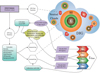Fig. 1.

Flowchart of our sub-grid procedures applied to the SPH to simulate FIR line emission in post-processing. This flowchart is similar to the one presented in Paper I; the main difference is the added H II regions as a new ISM phase. The dashed lines connect the gas and star environments to the ingredients of the model.

In Paper I we used starburst99 to calculate the ISRF from the stars close to gas particles (less than the smoothing length). Here we also used the spectrum from starburst99 to calculate the emission from H II regions. To generate this spectrum, we adopted the Geneva stellar models (Schaller et al. 1992) with standard mass loss for five metallicities (Z = 0.001, 0.004, 0.008, 0.020, and 0.040). We split starburst99 grid values in young (≤100 Myr) and old ages (> 100 Myr) to improve our estimations at younger ages. For young ages we estimated the parameters every 1 Myr, while for old ages we calculated 100 steps on a logarithmic scale up to 10 Gyr. We assumed a total stellar mass of 10⁴ M_⊙, with a Kroupa initial mass function (IMF). Therefore, to match the new mass resolution of 10⁴ M_⊙ from the starburst99 models, the original SPH star particles of the simulated galaxies were further divided into a number of ‘synthetic’ stellar clusters. The ages of the synthetic stellar clusters were drawn randomly from an exponential distribution, with the maximum age set to be the original ages of the parent SPH particles. This step was used to include younger stellar clusters that are not represented by a single age³. By doing this we avoided the poor sampling of star formation that can affect luminosity estimates, especially in H II regions.

We used a photoionisation model from CLOUDY to simulate the line emissivities of H II regions based on starburst99 spectra of their underlying stellar populations. We calculated the stellar atmospheres or spectral energy distributions (SEDs) in the photoionisation models for a given age, metallicity, and the ionising photon flux (Q). In this way the stellar age and metallicity from the star SPH particles were used to obtain Q coming from a stellar cluster from the starburst99 grids. Thus, we used these three physical parameters (age, metallicity, and Q) to construct spherical clouds where the emissivities depend only on them. The range of values for these parameters is presented in Table 3, totalling 25 200 grid points for all redshifts in this work.

Table 3.

Sampling of the properties of H II regions in the CLOUDY grid in this work.

In terms of the structure, we assumed a fixed density of ∼30 cm⁻³ to resemble classical H II regions similar to the Strömgren sphere, where densities are in the range of 10–100 cm⁻³ (Draine 2011). Choosing a higher or lower density affects the H II contribution to some lines, as described in Sect. 5. In ionisation balance the Strömgren radius is

$\begin{matrix} R_{Str} = {(\frac{3 Q}{4 π n {(H)}^{2} α_{B}})}^{1 / 3}, \end{matrix}$ $\begin{aligned} R_{\mathrm{Str} } = \left( \frac{3 Q}{4\pi \, n(\mathrm{H} )^{2}\, \alpha _{\rm B}} \right)^{1/3}, \end{aligned}$ (9)

where Q is the ionising photon flux in units of s⁻¹, n(H) is the total hydrogen number density in units of cm⁻³, and α_B is the Case B recombination rate coefficient.

These H II regions are radiation bound in terms of ionised hydrogen. Once the ratio of ionised hydrogen to the total hydrogen density drops below 5%, the calculation stops, which defines the outer radius. The inner radius was set to 1% of the expected Strömgren sphere radius (Eq. (9)), as in Yang & Lidz (2020), allowing us to obtain ultracompact H II regions, which can have sizes of ∼0.03 pc (Kurtz 2005). We calculated the emissivities without further iteration on the assumed density, which is adequate for clouds with densities typical of H II regions (Ferland 1996). For the rest of the configuration parameters in CLOUDY we used the same configuration used by Ploeckinger & Schaye (2020, Table C1), which is the same used for the optically thin and shielded gas grids (as described in Sect. 2.2).

The starburst99 outputs were also used to calculate the L_FUV and Q for each star SPH particle. Thus, the look-up luminosity tables from CLOUDY were used to interpolate the star SPH particles in terms of age, metallicity, and Q. As a result, we obtained the respective H II luminosity for each star particle for the FIR lines. This luminosity was then used as part of the total contribution of the ISM phases (DIG + neutral atomic gas + dense molecular gas + H II regions) for a given simulated galaxy.

3. Individual FIR line luminosities

In this section we present predictions for individual lines from our model and compare them with the observations. For each line we first examine how its luminosity varies as a function of SFR at different cosmic epochs. Our predictions of the line luminosity–SFR relation are then compared with observations collected and homogenised from previous studies (see Appendix A). Next, we investigate the contribution to the line luminosities from each of the ISM phases (i.e. the DIG, H II regions, neutral atomic and dense molecular gas). In this paper we mainly discuss the results of the five FIR lines, [C II] 158 μm, [O I] 63 μm, [N II] 205 μm, [O III] 88 μm, and [N III] 57 μm, as the other three lines (listed in Table 1) behave similarly to their above-mentioned pairs (e.g. [O III] at 52 μm is similar to [O III] at 88 μm). We have released all data in a Zenodo repository, as described in Appendix B.

3.1. [C II] 158 μm

3.1.1. The L_{[C II]}–SFR relationship

Arguably, the most important and brightest of the FIR lines is [C II] at 158 μm. This line exhibits a clear trend with SFR (e.g. Stacey et al. 1991, 2010; Brauher et al. 2008). Therefore, it is often used as a SFR tracer at different redshifts (e.g. De Looze et al. 2014; Herrera-Camus et al. 2015; Schaerer et al. 2020). In Fig. 2 we show the relationships between [C II] line luminosity (L_[C II]) and SFR for the seven redshift slices analysed in this work. We compare the predictions from the EAGLE simulations REF-L100N1504 and RECAL-L0025N0752 with predictions from other simulations (Olsen et al. 2015, 2018; Katz et al. 2022), semi-analytic models (Lagache et al. 2018; Popping et al. 2019) and empirical linear relationships derived from observations (De Looze et al. 2014; Schaerer et al. 2020). We also plot the linear relationships (derived independently for each redshift slice) that we infer from our model (see Appendix C) and extrapolate them (assumed to be linear) outside the dynamic range covered by the simulations, but within 10^−3.5M_⊙ yr⁻¹ < SFR < 10^3.5 M_⊙ yr⁻¹. With this extrapolation we can compare the observations with high SFR values that the simulations do not cover. This is necessary as high-z observations generally only include galaxies with very high SFR due to current sensitivity limits. In general, the agreement between our model predictions, observations, and other simulations/models is reasonable, considering the typical scatter of ∼0.4 dex (De Looze et al. 2014), especially at z = 0 and z = 6 where there are more observational constraints available. In Sect. 5, we present further discussions on issues such as simplifications in our sub-grid ISM model, limitations of the EAGLE simulation, and systematic effects in observations that could potentially have an impact on the comparison between model predictions and observational data for all lines modelled in this paper.

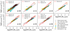Fig. 2.

SFR–L_[C II] relation for all redshift slices used in this work. The obtained relations from the EAGLE simulations REF-L100N1504 and RECAL-L0025N0752 are compared with predictions from other simulations (Olsen et al. 2015, 2018; Katz et al. 2022), semi-analytic models (Lagache et al. 2018; Popping et al. 2019), and linear relations derived from observations (De Looze et al. 2014; Schaerer et al. 2020). The linear relations inferred from our models are shown as black solid lines over the dynamic range covered by the simulations and extrapolated (assumed to be linear) to lower and higher SFRs as black dotted lines, with the grey shaded area representing the 1σ error. Collections of observational data (Appendix A) are plotted as grey squares for detections and as grey triangles for upper limits. For lensed galaxies the symbols are plotted in orange, and the upper limits that affect both the SFR and luminosity are plotted as diamonds.

In Paper I we showed that the L_[C II]–SFR relation at z = 0 could be reproduced reasonably well with a model similar to the one implemented in this work (i.e. with the added H II regions as the main difference). Therefore, it is not surprising that the current model still reproduces this L_[C II]–SFR relation. Compared to Popping et al. (2019), the only other model that covers the same redshift range as this work for [C II], our predicted L_[C II]–SFR relation has a much flatter slope. Especially at z = 1–3, the differences in the slopes can lead to up to ∼1.5 dex change in L_[C II] at SFRs around 1000 M_⊙ yr⁻¹, but the relations are more similar at other redshifts. Potential causes for these discrepancies may reside in the different galaxy formation physics in EAGLE and the Santa Cruz SAM used in Popping et al. (2019), as well as differences in the ISM models. However, a detailed comparison of the two galaxy formation models and the two ISM models in post-processing is beyond the scope of this work.

At z = 2 the linear relationship that Olsen et al. (2015) predicted from seven simulated galaxies shows a behaviour similar to that described in Popping et al. (2019) and agrees with the estimated scatter of our linear regression (∼0.2 dex) at SFRs around 1 M_⊙ yr⁻¹. Over the redshift range z = 1–3, the extrapolation of our relation shows a potential small offset compared with observations. However, this discrepancy is not significant because it takes into account the small sample size, large scatter (around 0.5 dex), potential bias towards galaxies with high line luminosities, and systematics in deriving luminosities and SFR. Furthermore, altering the assumptions in our modelling process could affect our predictions, as we show in Sect. 5.

At z = 4–6, most of the models and observations closely match the linear relationships derived from our predictions. Similar model predictions from Vallini et al. (2015) and Leung et al. (2020), and observations presented by Carniani et al. (2020), which are not shown in the plot, also agree at z = 6, indicating that the SFR–L_[C II] relationship can be tight at higher redshift, even if there is some scatter in the data related to observational errors (Schaerer et al. 2020). This demonstrates that our physically motivated model of the sub-grid ISM provides a reasonably good framework not only for estimating the luminosity of [C II] in the local Universe but also up to z = 6.

3.1.2. [C II] deficit

Although a linear L_[C II]–SFR relation is commonly assumed, observations of local galaxies show a decrease in L_[C II] at IR luminosities above 10¹² L_⊙ (i.e. the [C II] deficit; e.g. Díaz-Santos et al. 2017; Herrera-Camus et al. 2018a). However, recent observations of z > 4 galaxies show no evidence of such a deficit (e.g. Matthee et al. 2019; Carniani et al. 2020; Schaerer et al. 2020). In Ramos Padilla et al. (2021), we examined this deficit by comparing the L_[C II]–SFR relation with deviations from the star-forming main sequence (MS), following Herrera-Camus et al. (2018a). In this work we compare the L_[C II]/SFR ratio with the offset from the MS (ΔMS) in Fig. 3. We estimate the specific SFR (sSFR = SFR/M_⋆) of our galaxies and normalise this value by the derived sSFR for the MS from Speagle et al. (2014), which gives us the ΔMS. We find that L_[C II]/SFR almost always decreases with increasing ΔMS, supporting the idea that starbursts may not follow the L_[C II]–SFR relation shown in Fig. 2 (Herrera-Camus et al. 2018a; Ferrara et al. 2019). Thus, L_[C II] may not be a good SFR tracer for starbursts, as we discuss further in Sect. 3.6.

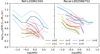Fig. 3.

[C II]/SFR ratio as a function of the offset from the star-forming main sequence ΔMS for the simulations REF-L100N1504 (left) and RECAL-L0025N752 (right). Shown are the median values of the different redshifts (solid lines) and their 25th and 75th percentiles (dotted lines). Only the bins with more than 3% of the total sample for the respective simulation are shown.

3.1.3. Contribution to L_{[C II]} from each ISM phase

In Fig. 4 we present the average contribution from the various ISM phases to L_[C II] at each redshift as a function of SFR of the galaxies in the RECAL-L0025N0752 simulation. The RECAL-L0025N0752 simulation was chosen because, with recalibration to the observed GSMF, it resembles more closely observed local galaxies, as discussed in Schaye et al. (2015) and De Rossi et al. (2017). In Paper I we also found this similarity by checking the contribution from atomic gas in [C II] line luminosity, which behaved more similarly to the observed local galaxies than the other EAGLE simulation boxes. In general, we find that most of the [C II] emission comes from the atomic phase, especially at z > 2, in agreement with the general assumption that neutral gas is the dominant ISM phase contributing to L_[C II] as estimated from observations (e.g. Croxall et al. 2017; Cormier et al. 2019) and suggested by models (e.g. Olsen et al. 2015, 2018; Lagache et al. 2018).

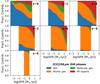Fig. 4.

Contribution from the different ISM phases to the [C II] emission line in RECAL-L0025N0752. The regions define the DIG (blue), neutral atomic gas (orange), dense molecular gas (green), and H II regions (red).

The contribution from neutral atomic gas to L_[C II] also changes with redshift, from ∼20–40% at z ≤ 1 to ∼70–90% at z ≥ 3. This change with redshift is connected with the evolving contribution from the DIG. At z = 0, the DIG dominates (i.e. the contribution is > 50%) in most galaxies with SFR < 0.1 M_⊙ yr⁻¹. At z = 2 the DIG contribution reduces to 30%, and at z = 6 it is negligible. This negligible contribution of the DIG at z = 6 does not agree with the estimated contribution of 44% by Olsen et al. (2018). This difference could be due to the different treatment in constructing the DIG clouds. We estimate the size of the DIG using a more physically based assumption, which leads to a more compact DIG, instead of using the smoothing length of the adopted simulation, as in Olsen et al. (2018). As our modelled L_[C II]–SFR relation shows a better agreement with observations, this may imply that a higher contribution from the atomic gas is needed to match the observed galaxies at z = 6. Therefore, our results favour the scenario where the atomic gas is the main ISM phase responsible for the L_[C II] at z = 6.

On the other hand, the fractional contribution from H II regions to L_[C II] reaches a maximum at z = 2, up to 80% of the line luminosity at high SFRs. This could be explained by the fact that H II regions trace young stars, and it is well known that the co-moving SFR density peaks at z ≈ 2 (Madau & Dickinson 2014). However, this could also be the result of our model assuming a fixed density for the H II regions. In general, the average contribution by H II regions is ∼20% of L_[C II] over all z < 4. For molecular gas, the contribution is on average ≲10% with a maximum at z = 0. In both the molecular and H II phases, we obtain larger contributions at higher SFR, consistent with the results in Olsen et al. (2015) and in Paper I. In Paper I we suggested that the reduced size of the neutral clouds, caused by increased SFRs, is the likely cause of the differences in the fractional contributions of ISM phases in L_[C II] (and possibly other lines as well). The presence of young stars at high SFR and the increase in dense environments (molecular phase) with redshift also play an important role. Most of these properties are related to star formation regulators such as stellar mass. Therefore, the change in the contributions of the various phases comes from the effect of star formation on the ISM, which explains its relation with the global SFR of a galaxy.

These predictions are not in agreement with recent results from Tarantino et al. (2021) on resolved regions of two local galaxies (M 101 and NGC 6946) which showed an almost negligible contribution from the ionised gas to L_[C II] (average upper limit of 12%). This disagreement may be related to the spatial constraints of the observations, as they focus on the arm regions where denser neutral gas is expected. For example, Pineda et al. (2018) estimated the L_[C II] contribution from different regions inside M 51. They found that the region between the arms (where the DIG is expected be located) accounts for ∼20% of the total L_[C II], compared to ∼80% from the arms and the nucleus. In our model we calculate the global properties of galaxies (in a 30 pkpc aperture). Thus, we expect a higher contribution from the DIG as this ISM phase can cover more extended regions. In general, contributions from different phases will depend on the scales over which we observe galaxies (Tarantino et al. 2021). Making a fair comparison between observations and simulations (e.g. by matching surface brightness limits) is beyond the scope of this paper.

In Fig. 5 we examine contribution from the ionised phases (i.e. DIG + H II regions) to [C II] as a function of metallicity (12 + log(O/H)). We also make a comparison with the empirical fitting function from Cormier et al. (2019), based on observations of the local Universe from their work and Croxall et al. (2017). For REF-L100N1504, our estimated fractional contributions are ∼10% higher than those inferred from the Cormier et al. (2019) fitting function, although at z = 0 our predictions can be 40% lower at high metallicities. In RECAL-L0025N0752, our predicted fractional contributions are always above the empirical fitting function, especially at z = 1 and z = 2, by around 40%. However, it is worth pointing out that it is very difficult to properly compare simulations with observations. The simulated galaxies may not have the same metallicity calibration as in Croxall et al. (2017) and Cormier et al. (2019), and the method by which contributions from the ionised gas are derived may be different. To summarise, our model shows a generally increasing contribution from the ionised phase to [C II] with increasing metallicity, which is qualitatively consistent with the observations.

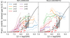Fig. 5.

Contribution from ionised gas phase to [C II]. Shown are the median values of the different redshifts (solid lines) and their 25th and 75th percentiles (dotted lines), and the observational data and the respective fit made by Cormier et al. (2019, black dashed line). The grey dots are the data from Croxall et al. (2017), while the red dots are from Cormier et al. (2019) at z = 0. Left panel: predictions of REF-L100N1504; Right panel: predictions of RECAL-L0025N0752. Only the bins with more than 5% of the total sample of galaxies for the respective simulation are shown.

3.2. [N II] 122 and 205 μm

3.2.1. The L_{[N II]}–SFR relationship

The [N II] emission lines at 122 and 205 μm are commonly used to trace ionised gas as its ionisation potential is only slightly above that of hydrogen. These lines can be used to disentangle the ionised gas contribution to the [C II] luminosity (e.g. Goldsmith et al. 2015; Ferkinhoff et al. 2015; Pavesi et al. 2016; Croxall et al. 2017; Cormier et al. 2019; Langer et al. 2021), as we do in this work. The relationship of these lines with SFR has been explored in the local Universe (e.g. Herrera-Camus et al. 2016; Zhao et al. 2016a). However, at higher redshifts we have very little observational data, especially for the 122 μm line. Consequently, we focus here on the [N II] 205 μm line. In Fig. 6 we plot [N II] 205 μm line luminosities as a function of SFR and compare them with the linear relations in the local Universe from Zhao et al. (2016a), Herrera-Camus et al. (2016), and Mordini et al. (2021). For the relation of Herrera-Camus et al. (2016, Eq. (10)), we assume the values of the collisional excitation coefficients from Tayal (2011) and abundances close to solar. For the relation of Mordini et al. (2021) we use the AGN sample (due to its statistical significance compared to the star-forming sample, N = 60 vs. N = 13), and adopt the Kennicutt & Evans (2012) conversion from infrared luminosities (L_IR) to SFR. In Mordini et al. (2021), it is shown that their AGN sample⁴ and star-forming galaxy (SFG) sample follow the same relation between the PAH 6.2 μm luminosity and the SFR derived from the total IR luminosity (their Fig. 6, panel a). The relations between the NII 205 μm line luminosity and the total IR luminosity for the AGN sample and the SFG sample are also very similar (their Fig. B8, panel b). Therefore, the NII line luminosity as a function of SFR (derived from the total IR luminosity) for these two samples should be very similar. In other words, it does not matter in practice whether we use the AGN sample or the SFG sample from Mordini et al. (2021) for comparison with our model predictions in this paper.

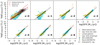Fig. 6.

Similar to Fig. 2, but for the [N II] 205 μm line. We also plot the linear relations from Zhao et al. (2016a), Herrera-Camus et al. (2016), and Mordini et al. (2021) at z = 0.

At z = 0 our predicted [N II] luminosities as a function of SFR follow a similar trend to the empirical relations of Zhao et al. (2016a) and Mordini et al. (2021). A potential reason for the difference of one to two orders of magnitude with respect to the Herrera-Camus et al. (2016) relation is that the assumption of solar abundances is incorrect⁵. If we assume a sub-solar abundance, then the Herrera-Camus et al. (2016) relation would be closer to our model prediction. At z = 1 and 2 our model is consistent with the observational upper limits. At 3 < z < 6, our model predictions agree fairly well with the observations. Most of the observational data at these redshifts come from the Cunningham et al. (2020) study which includes 40 gravitationally lensed galaxies observed with the Morita Atacama Compact Array (ACA) of ALMA, and thus the luminosities of these galaxies can depend strongly on the assumed lensing model. To summarise, our model shows a reasonable agreement with the observations, including the lensed galaxies after correction for magnification.

3.2.2. Contribution to L_{[N II]} from each ISM phase

In Fig. 7 we show the contribution of the different ISM phases to the [N II] 205 μm line. As expected from observations (e.g. Langer et al. 2021), the main contribution comes from the two ionised phases (i.e. DIG and H II regions). The relative dominance of these two phases evolves with redshift and SFR. At high SFR most of the luminosity comes from H II regions, while at low SFR most of the luminosity comes from the DIG phase. In the local Universe the contribution from the DIG dominates (∼80%) over that from H II regions. At 1 < z < 4, the contribution of the two phases is split roughly evenly. At z > 5 H II regions dominate the line emission, and at the highest SFRs H II regions contribute significantly more than the DIG. The transition between the phases (where DIG accounts for < 50% and H II regions > 50%) is around 1 M_⊙ yr⁻¹ at z = 0 and decreases to 0.1 M_⊙ yr⁻¹ at z = 6. There is also a very small (almost negligible) contribution from the atomic phase (< 4%) at some redshifts.

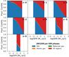Fig. 7.

Contribution from the different ISM phases to the [N II] emission line at 205 μm in RECAL-L0025N0752. The colour-coding is the same as in Fig. 4.

3.3. [O I] 63 and 145 μm

3.3.1. The L_{[O I]}–SFR relationship

The [O I] emission lines at 63 and 145 μm trace warm gas in neutral clouds and are commonly detected in galaxies in the local Universe (Malhotra et al. 2001). However, the 145 μm line is fainter than the 63 μm line due to its lower spontaneous decay rate and higher upper level energy (Goldsmith 2019). As with [N II], here we focus on the brighter [O I] emission line at 63 μm.

In Fig. 8 we present predictions of [O I] 63 μm line luminosity as a function of SFR at different redshifts. Our model at z = 0 agrees well with the local relations of De Looze et al. (2014) and Mordini et al. (2021). For the relation of Mordini et al. (2021), we use the star-forming sample, adopting the conversion from L_IR to SFR from Kennicutt & Evans (2012). At z > 1 extrapolations of the linear fits to our model predictions are consistent with the observational upper limits. There are only a few detections at z = 2, 3, and 6 that can be directly compared with our predictions. There are seven detections in the z = 2 bin, of which five are > 0.5 dex from the extrapolated linear fit. However, all of these galaxies are lensed (Brisbin et al. 2015), and no corrections have been applied to correct for lensing because the magnification factors are unknown (see also Zanella et al. 2018). Therefore, it is reasonable to treat these five measurements as upper limits. In the other redshift bins, we observe a reasonable agreement with the linear relationship because the lensing magnification has been taken into account (Rigopoulou et al. 2018; Zhang et al. 2018; Rybak et al. 2020).

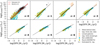Fig. 8.

Similar to Fig. 2, but for the [O I] 63 μm line. We present the linear relations estimated by De Looze et al. (2014) and Mordini et al. (2021) at z = 0.

A few other models (not shown in the plots) show similar results. For example, Olsen et al. (2018) predict the emission of 30 simulated galaxies at z = 6 in the MUFASA cosmological simulation. All of their galaxies have SFR ∼ 10 M_⊙ yr⁻¹ and L_[O I] ∼ 10⁸ L_⊙, very similar to our estimations of the REF-L100N1504 simulation. However in an updated model, Olsen et al. (2021) use the SIMBA cosmological simulation at z = 0, and their predicted [O I] 63 μm luminosities are 1.2 dex above the De Looze et al. (2014) relation shown in Fig. 8. This contrasts with our model, which exhibits better agreement with De Looze et al. (2014) and Mordini et al. (2021) at z = 0, with a difference of ∼0.1 dex at log(SFR[M_⊙ yr⁻¹]) = 1. We conclude that the model predictions presented in this work provide a better match with observations across a wide range of redshifts than previous models that only focus on a single redshift slice.

3.3.2. Contribution to L_{[O I]} from each ISM phase

Contributions to the [O I] 63 μm line come mainly from neutral clouds (i.e. neutral atomic gas and dense molecular gas), as shown in Fig. 9. At z = 0, the contribution to L_[O I] from molecular gas is ∼40% while from atomic gas it is ∼39%. The contribution from molecular gas decreases, while that from atomic gas increases with increasing redshift. The contributions from the other phases are negligible, especially for the H II regions. On average the contribution from the DIG is < 10%. However, it can be very high (> 80%) in galaxies with very low SFR (< 10⁻² M_⊙ yr⁻¹) in the local Universe. At z ≥ 3 the molecular fraction, which is calculated from the line luminosity in the region defined by the radius at which the transition from atomic to molecular hydrogen occurs, in the Plummer profile (Eq. (31) in Paper I) is very low. At those redshifts, even though the average density of the neutral cloud is higher than in the local Universe, the ISRF is also high, which causes the dominant emission to come from the atomic gas instead of the molecular gas. These results support the understanding that the [O I] 63 μm line originates in warm neutral environments (Malhotra et al. 2001; Goldsmith 2019) even in high-z galaxies (z ∼ 6).

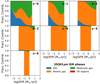Fig. 9.

Contribution from different ISM phases to the [O I] emission line in RECAL-L0025N0752.

3.4. [O III] 52 and 88 μm

3.4.1. The L_{[O III]}–SFRrelationship

The [O III] emission lines at 52 and 88 μm are the best tracers of ionised gas in the FIR. These lines may be used as SFR tracers as they come mainly from young stars (e.g. Ferkinhoff et al. 2010; De Looze et al. 2014; Inoue et al. 2014; Harikane et al. 2020; Yang & Lidz 2020; Yang et al. 2021b). The [O III] 88 μm line is a popular observational target as it may be brighter than [C II] in galaxies around the reionisation epoch (Inoue et al. 2014, 2016; Bouwens et al. 2022). Here we focus on the [O III] 88 μm line as there are more observational data for this line. In Fig. 10 we present our predicted [O III] 88 μm line luminosities as a function of SFR from REF-L100N1504 and RECAL-L0025N0752. We also make a comparison with observations of individual galaxies and linear relations derived from observations (De Looze et al. 2014; Harikane et al. 2020; Mordini et al. 2021) and other numerical models (Olsen et al. 2018; Katz et al. 2022; Kannan et al. 2022).

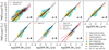Fig. 10.

As in Fig. 2, but for the [O III] 88 μm line. The obtained relations from the EAGLE simulations are compared with relations derived from simulations (Olsen et al. 2018; Katz et al. 2022; Kannan et al. 2022) and observations (De Looze et al. 2014; Harikane et al. 2020; Mordini et al. 2021). Linear relations inferred from our models using only H II regions are shown as indigo solid lines over the dynamic range covered by the simulations and extrapolated to lower and higher SFRs as indigo dotted lines; the shaded area represents the 1σ error (see Appendix C).

Our predicted L_[O III]–SFR relation agrees well with observations at z = 0, although it seems that our predicted relationship is steeper than some relations found in the literature and observations at z = 2, z = 3, and z = 4. At z = 0, we compare our model with the predictions of De Looze et al. (2014) and Mordini et al. (2021). For the relation of Mordini et al. (2021), we use the star-forming sample assuming the conversion from L_IR to SFR of Kennicutt & Evans (2012). The De Looze et al. (2014) empirical relation appears to have a flatter slope than our model, separated by about 0.3 dex at SFR = 10 M_⊙ yr⁻¹. The reason for this difference is that at low SFRs our luminosity predictions coming from H II regions drop off sharply for both simulations (see discussion in the next subsection), leading to a steep slope, even though our predicted L_[O III] values agree with the observational data at SFR = 1 M_⊙ yr⁻¹. If we estimate the linear relationships using only the luminosity coming from H II regions in simulated galaxies where they dominate (indigo lines), we find that the fit improves significantly at z = 0, which may provide a more physical reason for the difference in fit.

At z = 2–4, due to the small size of the observational datasets, it is very difficult to assess the level of agreement between the observations and our model predictions. There is fairly good agreement in some cases, but there are a few exceptions too. For example, the galaxy AzTEC 1 (Tadaki et al. 2019) is located 1.5 dex below the extrapolation at z = 4. This discrepancy is not related to lensing, but rather to a very low [O III]/[C II] ratio compared to SPT-S J041839-4751.8 (De Breuck et al. 2019) that lies close to our relation. Thus, the galaxy AzTEC 1 may be an outlier, and very different physical conditions can shift its position in the L_[O III]–SFR relation, as we discuss further in Sect. 4. At z = 5 we compare our results with those of Katz et al. (2022), which show a similar slope but lower L_[O III] (by ∼1 dex). At z = 6 the Katz et al. (2022) model and the Olsen et al. (2018) model both underestimate L_[O III] relative to the observations by 0.7 dex at SFR ∼ 100 M_⊙ yr⁻¹. In contrast, our model agrees very well with the observations and with the linear relation from Harikane et al. (2020). It is also interesting to note that the numerical results of Kannan et al. (2022) are very similar to our work, with the difference being a slightly higher slope in their work (resulting in a difference of 0.3 dex at SFR ∼ 10 M_⊙ yr⁻¹).

3.4.2. Contribution to L_{[O III]} from each ISM phase

In Fig. 11 we show that the ionised phase is the only contributor to L_[O III], as expected. The dominant phases are the H II regions at most redshifts. However at z = 0 the emission from the H II regions drops sharply with decreasing SFR. The reason for this sharp drop is the low ionising photon flux coming from the star SPH particles in the simulated galaxies at low SFR. This sets the [O III] line luminosities from the H II regions to almost negligible values compared to the DIG, which explains the trend observed in z = 0. At z = 1, the lack of ionising photon flux affects galaxies less than at z = 0, and at these redshifts the H II regions dominate (72%) over the DIG (28%). For redshifts from z = 2 to 6 the contribution from the H II regions changes from 85% to 99%.

Fig. 11.

Contribution from different ISM phases for the [O III] emission line in RECAL-L0025N0752. The colour-coding is the same as in Fig. 4.

3.5. [N III] 57 μm

3.5.1. The SFR–L_{[N III]} relationship

The [N III] emission line at 57 μm is very similar to the [O III] 88 μm emission line, due to its excitation properties (Table 1). Both trace H II regions, with the difference that [N III] is fainter in galaxies with sub-solar metallicities (e.g. Nagao et al. 2011; Rigopoulou et al. 2018). The relation between the SFR and L_[N III] is less well known than the other FIR emission lines. In Fig. 12 we compare our predicted L_[N III]–SFR relation from the EAGLE simulations with the observations and the empirical relation at z = 0 by Mordini et al. (2021) in AGN galaxies (as there is no star-forming sample), again adopting the conversion from L_IR to SFR in Kennicutt & Evans (2012).

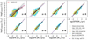Fig. 12.

As in Fig. 10, but for the [N III] 57 μm line. We present the linear relations estimated by Mordini et al. (2021) at z = 0.

At z = 0, our model predictions agree well with the observations, with a mean offset of 0.2 dex (within the observational scatter). However, the L_[N III] predictions have the same problem as the L_[O III] predictions: the low ionising photon flux coming from SPH star particles in simulated galaxies at low SFR. This leads to a steeper relation of L_[N III] with SFR than that of Mordini et al. (2021), which follows the other observational results. At z ≥ 1 (even though there is not much information), we find that extrapolations of our linear fits are consistent with the upper limits and detections in two galaxies at z ≈ 2 (H-ATLAS J091043.1-000321, Lamarche et al. 2018) and z ≈ 3 (HERMES J105751.1+573027, Rigopoulou et al. 2018). These two galaxies have been corrected for magnification (using a magnification factor of 11.5 and 10.9, respectively).

3.5.2. Contribution to L_{[N III]} from each ISM phase

The contributions from the ISM phases to the [N III] 57 μm emission line are very similar to the [O III] 88 μm line, as shown in Fig. 13. The exact percentages of the two dominant ionised ISM phases (the DIG and H II regions) differ. At z = 0 the contribution from the DIG and H II regions to L_[N III] amounts to 38% and 62%, respectively. These percentages change to 15% and 85% at z = 2, and 8% and 91% at z = 4. Finally, at z = 6 the H II regions are almost the sole ISM phase contributing to L_[N III].

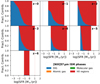Fig. 13.

Contribution from different ISM phases to the [N III] line luminosity in RECAL-L0025N0752.

3.6. Summary of FIR line luminosities

The relationships of the SFR with the different FIR line luminosities presented in Sects. 3.1–3.5 depend on redshift (Figs. 2, 6, 8, 10, and 12). We assume a SFR dependency in the linear fits of our line predictions (Eq. (C.1)), which shows a reasonable agreement with the observations. To quantify how these FIR lines and their dependence on SFR evolve with redshift, we plot in Fig. 14 the ratio of the line luminosity to SFR (L/SFR) versus redshift for the eight lines in this work.

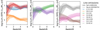Fig. 14.

Evolution of the line luminosity-to-SFR ratio with redshift for the FIR lines modelled in this work. Shown are the median values from RECAL-L0025N0752 (dotted lines) and REF-L100N1504 (solid lines). The shaded regions correspond to the 25th and 75th percentiles.

First, we compare the results of the two simulations REF-L100N1504 and RECAL-L0025N0752. Taking into account the scatter in the predictions, we find a reasonable agreement between them, even though some physical properties of the galaxies in the simulations are different and are derived from idealised models. For example, the calibration of the simulation parameters could be missing some physics that is not yet well understood and may affect the final simulation outputs (which may be based on observations that do not yet contain information for all relevant physical processes). We discuss these systematics in Sect. 5.

The redshift evolution of the L/SFR ratio is almost flat for most lines at z ≥ 4. At 1 < z < 3, however, there are bigger changes in L/SFR. For example, the [O III] lines have higher L/SFR values at z = 2 that decrease sharply towards z = 0, by almost a factor of 10. The opposite occurs for [C II], where at z = 2 the L/SFR ratio has lower values than at other redshifts, although the difference is < 0.5 dex. These changes are likely related to evolving ISM phases in galaxies during ‘cosmic noon’, where the cosmic star formation history reaches its peak at z ≈ 2 and half of the stellar mass in the local Universe was formed (Madau & Dickinson 2014; Förster Schreiber & Wuyts 2020).

The two [O III] lines have a similar shape in Fig. 14, which explains why either line can be used to constrain gas density and metallicity at high-z (Yang et al. 2021b). The [N II] pair shows a similar behaviour; the main difference resides in the value of L/SFR at z = 0, although the scatter is particularly large at this redshift. This could be important when estimating electron densities from observations using the ratio of the two [N II] lines (Croxall et al. 2017; Langer et al. 2021). Finally, for both [O I] lines, we see a clear difference of ∼1.15 dex over most of the redshift range, which is expected from theoretical models. If the difference in [O I] luminosities is > 1.15 dex, it may indicate higher kinetic temperatures (> 400 K) and/or lower gas densities (≲10 cm⁻³) in observations (Goldsmith 2019).

We can check which FIR line would be the best SFR tracer. The line showing the least variation with z is [C II]. However, this tracer may not be ideal in some cases. Observations, analytical models and simulations (e.g. Schaerer et al. 2020; Popping et al. 2019; Carniani et al. 2020) suggest that there might be a weak redshift evolution in the L_[C II] versus SFR relation. Our model predicts a slight evolution, but less than in the other lines. The evolution may be related to the star formation processes in starbursts, as shown in Fig. 3, and in galaxies during cosmic noon. The regulation of these star formation processes is reflected in the changes of the ISM phases (Fig. 4), which tend to be more stable in the case of L_[C II]. Another possible SFR tracer is L_[O III], which can be equal to or brighter than L_[C II] in some redshift ranges (e.g. Arata et al. 2020; Carniani et al. 2020; Vallini et al. 2021; Bouwens et al. 2022; Katz et al. 2022). Our L_[O III] predictions at z = 0 may be underestimated at low SFR (see Sect. 3.4.2), which explains the decrease in the median L/SFR value. It is also possible to use L_[O III] together with L_[O I] at 63 μm as a SFR tracer (Mordini et al. 2021) to balance the neutral and ionised ISM components in these lines. However, this would require having access to both lines at z < 4 to confirm the trends in Fig. 14. The [O I] 63 μm line, which has properties similar to those of the [C II] line, could also be used to trace SFR (Katz et al. 2022). Both our work and Olsen et al. (2018) predict that [O I] is brighter than [C II] at z = 6 and so is more easily observed. To summarise, L_[C II] may be the best SFR tracer across the entire redshift range of this work (z = 0–6), but at high redshifts other lines such as [O III] and [O I] are also very useful.

4. Diagnostic diagrams using FIR lines

We now examine our predictions of FIR emission line strengths from the EAGLE simulations using diagnostic diagrams. Typically, diagnostic diagrams use line ratios that reflect the physical conditions of the ISM. In this work, we focus on two diagnostic diagrams. One normalises the line luminosity with SFR for [C II] and [O III] at 88 μm (Harikane et al. 2020). The other uses the ratios between [C II]/[O III] and [N II]/[O I], based on the [O III], [N II], and [O I] lines at 88 μm, 205 μm, and 63 μm, respectively. With these two diagnostic diagrams we investigate whether these ratios trace physical properties of the ISM, such as radiation field and density. Other FIR line ratios are also of great interest for different types of studies (e.g. Sect. 3.3 of Cormier et al. 2015). We therefore make our line predictions of the simulated EAGLE galaxies publicly available, as described in Appendix B. Similar FIR diagnostic diagrams, such as those in De Breuck et al. (2019) and Li et al. (2020) are not discussed here, but plots are provided as supplementary material⁶.

4.1. L_{[O III]}/SFR versus L_{[C II]}/SFR

We compare our predictions with the observations (Appendix A) and results from the latest version of the SIGAME framework in Olsen et al. (2021). The latest version uses two boxes of 25 cMpc and 100 cMpc in the local Universe from the SIMBA simulations (Davé et al. 2019), together with the SKIRT (Camps & Baes 2020) radiative transfer code and CLOUDY (Ferland et al. 2017) to predict lines. Olsen et al. (2021) find that their L_[C II] predictions appear to be an extension to higher SFRs of our predictions in Paper I. However, SIGAME tends to have higher line luminosities relative to the L_[C II]–SFR relation (their Fig. 11). In Fig. 15, we compare L_[O III]/SFR versus L_[C II]/SFR from our model with the observations and the SIGAME predictions. In the local Universe, our predictions occupy a similar range to the observations, with 6.5 < log(L_[C II]/SFR) < 7.6 and 5.8 < log(L_[O III]/SFR) < 7.6. However, most of the simulated galaxies are above or below the observations. In contrast, SIGAME tends to have very high L_[C II]/SFR, peaking at an order of magnitude higher than the observed galaxies and our model. This is expected as Olsen et al. (2021) show that the SIGAMEL_[C II]/SFR predictions are higher than those described in Paper I, which are similar to those in this work. The SIGAMEL_[O III]/SFR values are similar to our predictions, with 6.0 < log(L_[O III]/SFR) < 8.

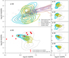Fig. 15.

Diagnostic diagram for L_[O III]/SFR and L_[C II]/SFR, similar to that presented in Harikane et al. (2020; shown as red filled dots for detections and triangles for upper limits). The cyan and olive contours show the model predictions from REF-L100N1504 and RECAL-L0025N0752. Shown is a comparison between the observational data (black squares) and the SIGAME predictions (Olsen et al. 2021) for the local Universe in 25 Mpc and 100 Mpc simulation boxes (purple and brown contours). The panels with redshifts above zero show the z = 0 RECAL-L0025N0752 estimations as grey dashed contours.

At z > 0 there are very few observations. At z = 2 we have two measurements for H-ATLAS J091043.0-000322, from Herschel observations using different data reduction methods in Zhang et al. (2018) and Lamarche et al. (2018). The ALMA observations in Lamarche et al. (2018) show that the [C II] luminosity is around half of the Herschel measurement, but this difference cannot be fully explained. Assuming the galaxy lies somewhere between the two measurements, it would be consistent with our predictions from RECAL-L0025N0752. At z = 3 we have three measurements for SDP 81 (Valtchanov et al. 2011; De Looze et al. 2014; Zhang et al. 2018) and one for HLock01 (Rigopoulou et al. 2018). For SDP 81, two of the measurements coincide (De Looze et al. 2014 use the values from Valtchanov et al. 2011): the empty squares with log(L_[C II]/SFR) ∼ 7.6. The other measurement comes from Zhang et al. (2018) using a different data reduction method, which is the leftmost point in the z = 3 panel. Both SDP 81 and HLock01 are close to the model predictions of RECAL-L0025N0752. At z = 4 the measurements for two galaxies, SPT-S J041839-4751.8 (De Breuck et al. 2019) and AzTEC 1 (Tadaki et al. 2019), are consistent with our predictions. Finally, at z = 6 we have measurements for two galaxies, [DWV2017b] CFHQ J2100-1715 companion (Walter et al. 2018) and [MOK2016b] HSC J121137.10-011816.4 (Harikane et al. 2020). The former is in the same region as our model; the latter falls in the same upper region as SPT-S J041839-4751.8 in the z = 4 panel. These two galaxies have SFRs around 100 M_⊙ yr⁻¹ and have L_[O III] higher than their respective companions in their panels. These high SFRs can explain their positions in the diagnostic diagrams.

4.2. L_{[N II]}/L_{[O I]} versus L_{[C II]}/L_{[O III]}

In Fig. 16 we compare our predicted [C II]/[O III] and [N II]/[O I] ratios with the observations and SIGAME predictions. At z = 0 our predictions, observations, and SIGAME predictions tend to be grouped in the region between − 0.5 < log(L_[C II]/L_[O III]) < 1.5 and − 1 < log(L_[N II]/L_[O I]) < 1. SIGAME matches most of the observational data, but misses the points around log(L_[C II]/L_[O III]) = 0 and log(L_[N II]/L_[O I]) = 0. Our model behaves similarly to Fig. 15, where most of the observations lie between the two regions for RECAL-L0025N0752, and REF-L100N1504. Our estimates with a simple ISM model are in the same parameter space as the observations. However, a completely fair comparison is challenging to make (for example due to different selection bias in the observations and simulations).

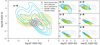Fig. 16.

Diagnostic diagram using four different FIR emission lines comparing the [C II]/[O III] ratio to the [N II]/[O I] ratio.

As we are using four FIR emission lines, there are very few observations to which we can make a comparison at higher redshifts. So far, the only galaxy with all four lines is SPT-S J041839-4751.8 at z = 4 (De Breuck et al. 2019). Our model matches the position of this galaxy, similar to the results presented in Fig. 15.

4.3. Impact of physical parameters

In Fig. 17 we use the line predictions of all modelled galaxies over all redshifts to examine the impact of eight parameters related to the physical conditions of the ISM: gas mass (M_gas), stellar mass (M_*), metallicity (Z/Z_⊙), sSFR, interstellar radiation field (ISRF), total hydrogen number density in the neutral clouds (n(H)_cloud), external pressure (P_ext), and radius of the neutral clouds (R_cloud). We also make a comparison with the observational dataset of Appendix A. The impact of almost all physical parameters is perpendicular to the observations because the predicted [C II]/SFR range is much smaller than the observations. Most of the simulated galaxies in the upper left corner of the observation contour tend to have higher M_gas, M_*, sSFR, ISRF, n(H)_cloud), and P_ext, and lower R_cloud. In addition, low values of M_* do not reach the bottom right limit of the observations and there is no clear trend in metallicity.

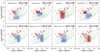Fig. 17.

Impact of physical parameters in L_[O III]88/SFR vs. L_[C II]/SFR. The RECAL-L0025N0752 model predictions combined over all redshifts are shown as as grey dashed contours and the compiled observations as green dashed contours. The colour-coded rectangles represent the area between the 25th and 75th percentiles from low (blue) to high (red) values for the given parameters: gas mass (M_gas), stellar mass (M_*), metallicity (Z/Z_⊙), sSFR, ISRF, total hydrogen number density in the neutral clouds (n(H)_cloud), external pressure (P_ext), and radius of the neutral clouds (R_cloud). The solid black lines connect the median values of each rectangle. Detections and upper limits from Harikane et al. (2020) are shown as red filled dots and triangles (as in Fig. 15), respectively.

Harikane et al. (2020) used L_[O III]/SFR versus L_[C II]/SFR to infer the physical properties of galaxies at z = 6–9. Using simple CLOUDY grids, they find that one probable reason for the location of some of their galaxies in the upper right region of the diagnostic diagrams is a high ionisation parameter (proportional to the ISRF), similar to what we find in Fig. 17. In terms of metallicity, Harikane et al. (2020) find that L_[O III]/SFR decreases with metallicity while L_[C II]/SFR does not change. We find the same result for L_[C II]/SFR, but the range of change of the L_[O III]/SFR ratio is not directly dependent on metallicity. In terms of density, Harikane et al. (2020) find that both ratios decrease with density, which we also find for L_[C II]/SFR but not for L_[O III]/SFR. A possible reason for this discrepancy is that L_[C II]/SFR depends mainly on density, while L_[O III]/SFR is more dependent on other physical parameters, for example metallicity, sSFR, and gas mass.

Figure 17 highlights the importance of the [C II] and [O III] emission lines (especially their ratios) in understanding the physical conditions of the ISM, as other recent studies have done (e.g. Harikane et al. 2020; Arata et al. 2020; Carniani et al. 2020; Vallini et al. 2021; Bouwens et al. 2022) and as we show below. We check its correlation with other lines that trace the neutral and ionised gas, such as the [N II]/[O I] ratio. We present the impact of the eight physical parameters on [C II]/[O III] versus [N II]/[O I] in Fig. 18. Interestingly, the bottom panels show a spoon-like shape, with most of the observed galaxies having low to moderate values of ISRF, n(H)_cloud, and P_ext, and moderate to high values of R_cloud. The opposite occurs in the region with low [C II]/[O III] (i.e. high ISRF, n(H)_cloud, and P_ext, and low R_cloud), which coincides with our predictions for z > 3 galaxies in Fig. 16. The parameter M_gas follows a similar trend to the parameters mentioned above, while M_* does not show a clear trend. The most intriguing trends in [N II]/[O I] versus [C II]/[O III] come from metallicity and sSFR. In terms of metallicity, [C II]/[O III] seems to be a good tracer for values close to solar, while [N II]/[O I] is a good tracer for metallicities below log(Z/Z_⊙)≲0.5, which agrees with some results for high-z galaxies (Arata et al. 2020). In terms of sSFR, both ratios do a good job in separating high and low sSFR in a zigzag pattern across the observations, supporting the idea that [C II]/[O III] can be used for starbursts (Vallini et al. 2021).

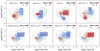Fig. 18.

Impact of the physical parameters in the diagnostic plot comparing the [C II]/[O III] ratio to the [N II]/[O I] ratio. The colour-coding and contours are similar to those in Fig. 17, but for the respective luminosity ratios.

We have shown that both diagnostic diagrams track the impact of the physical parameters in the simulated galaxies. Our model agrees with the observations in most of the parameter space, and in some cases with other simulations (e.g. SIGAME). Therefore, our model could be used to infer the physical parameters from FIR diagnostic diagrams. We note that the modelled FIR lines can also be used to study other types of problems. For example, [N II]/[C II] can be used to characterise different types of galaxies (e.g. Ultra-luminous infrared galaxies with L_IR > 10¹² L_⊙) in the local Universe (Farrah et al. 2013) and at high-z (Cunningham et al. 2020). The ratio of the two [O III] lines can be used to test the efficiency of black hole feedback, as was done with the IllustrisTNG simulations (Inoue et al. 2021). Similarly, [O III]/[N III] or [O III]/[N II] can be used as a metallicity indicator (e.g. Nagao et al. 2011; Rigopoulou et al. 2018; Fernández-Ontiveros et al. 2021).

5. Discussion

5.1. Model assumptions

Although our predicted line luminosities and ratios are in reasonable agreement with observations and other simulations, our physically motivated ISM model is based on a number of simplifying assumptions. Below we discuss the potential impact of some of these assumptions.

For neutral clouds and H II regions, we assume static spherical geometries to describe the densities and temperatures within those environments. This assumption is made for simplicity, although we know that these structures may not be spherical. Physical processes such as radiation destroy spherical geometries (Deharveng et al. 2010; Peñaloza et al. 2018), which may lead to rough or incorrect line predictions (Decataldo et al. 2020). However, approximations using mass distributions (Eq. (15) in Paper I) may smooth out these differences since cloud masses follow scaling relations that seem to be valid for observations at different redshifts (Dessauges-Zavadsky et al. 2019).

A problem with our line luminosities from H II regions is the assumed fixed density. We can increase the luminosity by increasing this density and vice versa. The use of different densities could have an impact on the contributions from DIG and H II regions, especially for [O III] and [N III] (see Figs. 11 and 13). This DIG–H II balance is still unclear in ionised lines, and although some estimates exist in the optical (e.g. Poetrodjojo et al. 2019), a change in this balance can lead to different metallicities, which may affect high-z studies (Sanders et al. 2017). In this work we calibrate the DIG phase with observations at z = 0 and use this calibration at higher redshifts, which may also bias the DIG–H II balance. Larger DIG clouds will have lower emissivities, which will reduce the DIG contribution to the line, making H II regions more important. Fortunately, the results presented in this work show that these assumptions seem to be in agreement with the observations, which may represent a likely first step in understanding the DIG–H II balance.

Finally, our predictions depend on CLOUDY lookup tables, which can give different emissivities depending on the assumed initial abundances or dust configurations (Ploeckinger & Schaye 2020). Different photoionisation models could lead to different interpretations of physical parameters based on line ratios, such as metallicity or the ionisation parameter (e.g. Ji & Yan 2022). Furthermore, the intrinsic thermodynamics may not be the same in terms of cooling and heating functions in cosmological simulations and photoionisation models like CLOUDY (Robinson et al. 2022). Thus, care must be taken when interpreting the lines predicted by our model.

5.2. Using EAGLE

Here we use the EAGLE simulation, and so our line predictions inherit the potential limitations of the simulation. One example is the lack of starbursts (Wang et al. 2019a), as discussed in Paper I, which restricts our comparison at z = 0 to SFR < 10 M_⊙ yr⁻¹ and similarly at z > 0 (Katsianis et al. 2017). At high SFRs we need to extrapolate the linear relations, and so care must be taken when using this extrapolation.

Another important physical property that affects our predictions is gas metallicity, usually studied through the gas-phase mass-metallicity relation (MZR). Bellstedt et al. (2021) show that the MZR in EAGLE, as measured by Zenocratti et al. (2020) at z = 0, does not behave similarly to other cosmological simulations or semi-analytical models. As shown in Fig. 4 of Bellstedt et al. (2021), the metallicities in EAGLE are around 12 + log(O/H)∼9 at 9 < log(M_*[M_⊙]) < 11, which is high compared to observations with metallicities from ∼8.5 to ∼9.2 in the same stellar mass range. This may affect the metallicity that can be derived from FIR lines if only z = 0 is used. However, MZR in EAGLE depends on resolution and box-size, due to the assumed AGN and star formation feedback (De Rossi et al. 2017). In Figs. 17 and 18 we find that some FIR line ratios can be useful for inferring metallicity. In the future it will be important to compare the FIR line predictions that trace metallicity with observations more consistently.

Although we base our predictions on EAGLE, we expect that similar physical models and/or cosmological simulations can be used to understand the gas properties with FIR lines. For example, Olsen et al. (2021) presented predictions obtained with a different gas fragmentation scheme using SIGAME, which are similar to observations and our predictions. However, most of the galaxies in SIGAME have higher SFR than those studied here. This difference is probably due to the different simulation used (i.e. SIMBA), which allows for the formation of starbursts. Therefore, although some physical assumptions are different for each model and are limited by the simulation used (e.g. Vallini et al. 2015; Lagache et al. 2018; Popping et al. 2019; Pallottini et al. 2019; Leung et al. 2020), we expect predictions (based on similar tools, e.g. SIGAME or CLOUDY) to behave similarly to those presented in this work.

5.3. Observational data

For comparison between observations and our model, we collected a heterogeneous sample of observed galaxies with FIR line information. We transformed the line luminosities to the same reference cosmology (Planck Collaboration XVI 2014) and estimated the SFR in most of the cases using the SFR–L_IR relation in Kennicutt & Evans (2012). However, there are other issues, as discussed below.

One issue is the adopted IMF, which is not always specified in papers. Assuming a star formation law that takes into account a standard IMF is a possible solution, as we have tried in this work. However, this may add additional uncertainties. For example, EAGLE uses an instantaneous SFR, which is different from the SFR averaged over the last 10 or 100 Myr typically used in observations. Another problem is that some of the SFR (or L_IR) may come from SED models rather than empirical relations using FIR photometric bands, such as IRAS, PACS, or SPIRE. In addition, IR luminosities can be integrated over different wavelength ranges, adding to the spread in SFR estimates (Förster Schreiber & Wuyts 2020) and leading to differences by factors between 1.1 and 1.7 (De Looze et al. 2014; Lagache et al. 2018). Another possibility is to use other tracers, such as Hα-, UV-, or radio-based SFRs (e.g. Wang et al. 2016, 2019b). However, in some cases, such as at high-z, it can be difficult to obtain such SFR estimates and other lines like [C II] come into play as a SFR tracer (Le Fèvre et al. 2020), as we have also shown in this work. In addition, there are systematic uncertainties in some of the line measurements, due to for example different instruments or calibrations, as shown by Lamarche et al. (2018) in H-ATLAS J091043.0-000322 (Sect. 4.1). Furthermore, apertures of different sizes (or shapes) in observations may affect the analysis of the fixed-size aperture we selected for the simulated galaxies (30 pkpc). For example, the balance between DIG and H II regions as main contributors to the ionised lines could depend on aperture (Mannucci et al. 2021). Finally, lensing can introduce a large uncertainty in the luminosities, and the magnification factor may also depend on the observed region of the galaxy (Lamarche et al. 2018). In this work, we highlight those galaxies for potential complications, but in general, they show reasonable agreement with our predictions.

6. Summary and conclusions

We have modelled FIR emission lines by post-processing EAGLE cosmological simulations and using CLOUDY look-up tables for line emissivities. We have predicted the luminosities of the eight most important lines in the FIR up to z = 6, using a physically motivated model that traces four different ISM phases: dense molecular gas, neutral atomic gas, diffuse ionised gas, and H II regions. We have also collected a sample of observed galaxies from the literature for comparison with our predictions. Our main conclusions are as follows:

Predictions from our model generally show reasonable agreement with observed galaxies in the FIR line luminosity–SFR relation within ∼0.5 dex over z = 0–6, which is comparable to typical observational errors. We made comparisons with different models, and found a similar level of agreement. We also model the line luminosity–SFR relation for each line with a linear relation, each of which shows a slight evolution with redshift.
We presented contributions from the four ISM phases to each line. These contributions change as a function of SFR. For the [C II] 158 μm line, the main contributor is the neutral atomic gas, with considerable contributions from H II regions at z = 1–4 and the DIG at z < 2, which may be related to metallicity. For the [N II] lines at 122 and 205 μm, the DIG contributes more than H II regions in the local Universe, but the opposite is true at high-z, where H II regions seem to dominate over the DIG. For the [O I] lines at 63 and 145 μm, the contribution of dense molecular gas is important in the local Universe. However, the atomic gas is dominant at high-z. Finally, for the [O III] lines at 52 and 88 μm and [N III] at 57 μm, we show that H II regions dominate, with important contribution from the DIG at low SFR in the local Universe.
We predict that [C II] may not be a good SFR tracer for starbursts since [C II]/SFR decreases as a function of the offset from the star-forming main sequence. However, compared to the other FIR lines, [C II] seems to be the best SFR tracer due to its weak redshift evolution. [O III] and [O I] may also be good SFR tracers. Nonetheless, our predictions of [O III] at z = 0 may be underestimated, and more observations of [O I] are necessary at z < 4 to confirm our predictions.
We compared our predictions in two diagnostic diagrams, and we find reasonable agreement with observations. We compared the L_[O III]/SFR and L_[C II]/SFR ratios and find that simulated galaxies at high-z tend to have higher L_[O III]/SFR ratios and slightly lower L_[C II]/SFR ratios than galaxies in the local Universe. We also compared the [C II]/[O III] and [N II]/[O I] ratios and find that simulated galaxies at high-z tend to have lower [C II]/[O III] and [N II]/[O I] ratios than local galaxies.
Finally, we examined the impact of physical parameters on the diagnostic diagrams. We find that L_[C II]/SFR and L_[O III]/SFR trace hydrogen density and ISRF well in the simulated galaxies. However, these ratios are not good metallicity tracers because L_[O III]/SFR does not evolve linearly with metallicity and L_[C II]/SFR does not change with metallicity. Furthermore, we find that [C II]/[O III] and [N II]/[O I] can be good metallicity and sSFR tracers. For example, [C II]/[O III] can trace metallicities close to solar and [N II]/[O I] below solar. On the other hand, we can identify systems with different sSFRs by means of both [C II]/[O III] and [N II]/[O I] ratios, which can be very useful for improving calibrations of [C II] as a SFR tracer.

In the future we expect to use this model and its predictions to understand the effect that AGN can have and that the physical parameters can have in these lines and their ratios. We have made our model predictions and collected observational sample publicly available to allow potential users to make a comparison with their work or interpret new observations. We anticipate that our predictions⁷ will also be useful in planning⁸ for future FIR missions (van der Tak 2023).

¹

From the power-law relationship between the SFR density and the density of interstellar gas $ρ_{SFR} = ρ_{gas}^{n}$ $\rho_{\mathrm{SFR}} = \rho_{\mathrm{gas}}^{\mathrm{n}}$ .

²

[O I] emission can come from the inner core. However, as our results show, the contribution of this inner core to the [O I] luminosity is usually very small.

³

A similar approach to achieve a finer sampling of the star formation history was used in Trayford et al. (2015).

⁴

The AGN sample in Mordini et al. (2021) excludes sources with total IR luminosities L_IR > 10⁴⁵ erg s⁻¹ in which severe contamination by the AGN may be present in L_IR and SFR estimates.

⁵

Compared to the relations of Zhao et al. (2016a) and Mordini et al. (2021), the N/H abundance that best matches the data is between the values of 0.03 and 0.16 with respect to solar abundance.

⁶

Zenodo repository at https://doi.org/10.5281/zenodo.6576202

⁷

https://sites.google.com/site/mexicanmillionmodels

⁸

http://www.astropy.org

⁹

These distances come from methods that use standard candles or rules, such as Cepheids and globular clusters.

¹⁰

GOALS sample at https://goals.ipac.caltech.edu

Acknowledgments

We thank Karen Pardos Olsen for providing the data from the SIGAME framework and the anonymous referees for helpful suggestions and comments. This research has made use of the 3Mdb database (Morisset et al. 2015) from which initial experiments to model H II regions were performed. This research made use of Astropy, a community-developed core Python package for Astronomy (Astropy Collaboration 2013, 2018), and several other Python packages, including numpy (Harris et al. 2020), pandas (McKinney 2010) and matplotlib (Hunter 2007). This research made use of R (R Core Team 2021), the SIMBAD database, operated at CDS, Strasbourg, France, and the NASA/IPAC Extragalactic Database (NED), which is funded by the National Aeronautics and Space Administration and operated by the California Institute of Technology. This research has made use of NASA’s Astrophysics Data System Bibliographic Services. The EAGLE simulations were performed using the DiRAC-2 facility at Durham, managed by the ICC, and the PRACE facility Curie based in France at TGCC, CEA, Bruyères-le-Châtel. We thank the Center for Information Technology of the University of Groningen for support and access to the Peregrine high performance computing cluster.

References

Abdullah, A., & Tielens, A. G. G. M. 2020, A&A, 639, A110 [NASA ADS] [CrossRef] [EDP Sciences] [Google Scholar]
Abdullah, A., Brandl, B. R., Groves, B., et al. 2017, ApJ, 842, 4 [Google Scholar]
Arata, S., Yajima, H., Nagamine, K., Abe, M., & Khochfar, S. 2020, MNRAS, 498, 5541 [NASA ADS] [CrossRef] [Google Scholar]
Aravena, M., Decarli, R., Walter, F., et al. 2016, ApJ, 833, 71 [NASA ADS] [CrossRef] [Google Scholar]
Armus, L., Mazzarella, J. M., Evans, A. S., et al. 2009, PASP, 121, 559 [Google Scholar]
Ashby, M. L. N., Mahajan, S., Smith, H. A., et al. 2011, PASP, 123, 1011 [CrossRef] [Google Scholar]
Astropy Collaboration (Robitaille, T. P., et al.) 2013, A&A, 558, A33 [NASA ADS] [CrossRef] [EDP Sciences] [Google Scholar]
Astropy Collaboration (Price-Whelan, A. M., et al.) 2018, AJ, 156, 123 [Google Scholar]
Bellstedt, S., Robotham, A. S. G., Driver, S. P., et al. 2021, MNRAS, 503, 3309 [NASA ADS] [CrossRef] [Google Scholar]
Béthermin, M., De Breuck, C., Gullberg, B., et al. 2016, A&A, 586, L7 [NASA ADS] [CrossRef] [EDP Sciences] [Google Scholar]
Béthermin, M., Fudamoto, Y., Ginolfi, M., et al. 2020, A&A, 643, A2 [Google Scholar]
Blitz, L., Fukui, Y., Kawamura, A., et al. 2007, in Protostars and Planets V, eds. B. Reipurth, D. Jewitt, & K. Keil (Tucson: University of Arizona Press), 81 [Google Scholar]
Bonatto, C., & Bica, E. 2011, MNRAS, 415, 2827 [NASA ADS] [CrossRef] [Google Scholar]
Bordalo, V., Plana, H., & Telles, E. 2009, ApJ, 696, 1668 [NASA ADS] [CrossRef] [Google Scholar]
Bouwens, R. J., Smit, R., Schouws, S., et al. 2022, ApJ, 931, 160 [NASA ADS] [CrossRef] [Google Scholar]
Brauher, J. R., Dale, D. A., & Helou, G. 2008, ApJS, 178, 280 [NASA ADS] [CrossRef] [Google Scholar]
Brisbin, D., Ferkinhoff, C., Nikola, T., et al. 2015, ApJ, 799, 13 [Google Scholar]
Bussmann, R. S., Pérez-Fournon, I., Amber, S., et al. 2013, ApJ, 779, 25 [NASA ADS] [CrossRef] [Google Scholar]
Camps, P., & Baes, M. 2020, Astron. Comput., 31, 100381 [NASA ADS] [CrossRef] [Google Scholar]
Capak, P. L., Carilli, C., Jones, G., et al. 2015, Nature, 522, 455 [NASA ADS] [CrossRef] [Google Scholar]
Carilli, C. L., & Walter, F. 2013, ARA&A, 51, 105 [NASA ADS] [CrossRef] [Google Scholar]
Carniani, S., Ferrara, A., Maiolino, R., et al. 2020, MNRAS, 499, 5136 [NASA ADS] [CrossRef] [Google Scholar]
Cheng, C., Cao, X., Lu, N., et al. 2020, ApJ, 898, 33 [NASA ADS] [CrossRef] [Google Scholar]
Cigan, P., Young, L., Cormier, D., et al. 2016, AJ, 151, 14 [NASA ADS] [CrossRef] [Google Scholar]
Cooray, A., Calanog, J., Wardlow, J. L., et al. 2014, ApJ, 790, 40 [NASA ADS] [CrossRef] [Google Scholar]
Coppin, K. E. K., Danielson, A. L. R., Geach, J. E., et al. 2012, MNRAS, 427, 520 [NASA ADS] [CrossRef] [Google Scholar]
Cormier, D., Lebouteiller, V., Madden, S. C., et al. 2012, A&A, 548, A20 [NASA ADS] [CrossRef] [EDP Sciences] [Google Scholar]
Cormier, D., Madden, S. C., Lebouteiller, V., et al. 2015, A&A, 578, A53 [CrossRef] [EDP Sciences] [Google Scholar]
Cormier, D., Abel, N. P., Hony, S., et al. 2019, A&A, 626, A23 [NASA ADS] [CrossRef] [EDP Sciences] [Google Scholar]
Cortés, J. R., Kenney, J. D. P., & Hardy, E. 2008, ApJ, 683, 78 [CrossRef] [Google Scholar]
Crain, R. A., Schaye, J., Bower, R. G., et al. 2015, MNRAS, 450, 1937 [NASA ADS] [CrossRef] [Google Scholar]
Croxall, K. V., Smith, J. D., Pellegrini, E., et al. 2017, ApJ, 845, 96 [Google Scholar]
Cunningham, D. J. M., Chapman, S. C., Aravena, M., et al. 2020, MNRAS, 494, 4090 [NASA ADS] [CrossRef] [Google Scholar]
Dalla Vecchia, C., & Schaye, J. 2012, MNRAS, 426, 140 [NASA ADS] [CrossRef] [Google Scholar]
Davé, R., Anglés-Alcázar, D., Narayanan, D., et al. 2019, MNRAS, 486, 2827 [Google Scholar]
Dayal, P., & Ferrara, A. 2018, Phys. Rep., 780, 1 [Google Scholar]
De Breuck, C., Weiß, A., Béthermin, M., et al. 2019, A&A, 631, A167 [NASA ADS] [CrossRef] [EDP Sciences] [Google Scholar]
Decarli, R., Walter, F., Neri, R., et al. 2012, ApJ, 752, 2 [NASA ADS] [CrossRef] [Google Scholar]
Decarli, R., Walter, F., Carilli, C., et al. 2014, ApJ, 782, L17 [NASA ADS] [CrossRef] [Google Scholar]
Decarli, R., Walter, F., Venemans, B. P., et al. 2017, Nature, 545, 457 [Google Scholar]
Decataldo, D., Lupi, A., Ferrara, A., Pallottini, A., & Fumagalli, M. 2020, MNRAS, 497, 4718 [NASA ADS] [CrossRef] [Google Scholar]
Deharveng, L., Schuller, F., Anderson, L. D., et al. 2010, A&A, 523, A6 [NASA ADS] [CrossRef] [EDP Sciences] [Google Scholar]
De Looze, I., Cormier, D., Lebouteiller, V., et al. 2014, A&A, 568, A62 [NASA ADS] [CrossRef] [EDP Sciences] [Google Scholar]
De Rossi, M. E., Bower, R. G., Font, A. S., Schaye, J., & Theuns, T. 2017, MNRAS, 472, 3354 [Google Scholar]
Dessauges-Zavadsky, M., Richard, J., Combes, F., et al. 2019, Nat. Astron., 3, 1115 [NASA ADS] [CrossRef] [Google Scholar]
Díaz-Santos, T., Armus, L., Charmandaris, V., et al. 2017, ApJ, 846, 32 [Google Scholar]
Dolag, K., Borgani, S., Murante, G., & Springel, V. 2009, MNRAS, 399, 497 [Google Scholar]
Draine, B. T. 2011, Physics of the Interstellar and Intergalactic Medium (Princeton University Press) [Google Scholar]
Duarte Puertas, S., Vilchez, J. M., Iglesias-Páramo, J., et al. 2017, A&A, 599, A71 [NASA ADS] [CrossRef] [EDP Sciences] [Google Scholar]
Evans, A. S., Solomon, P. M., Tacconi, L. J., Vavilkin, T., & Downes, D. 2006, AJ, 132, 2398 [NASA ADS] [CrossRef] [Google Scholar]
Faisst, A. L., Capak, P. L., Yan, L., et al. 2017, ApJ, 847, 21 [Google Scholar]
Farrah, D., Lebouteiller, V., Spoon, H. W. W., et al. 2013, ApJ, 776, 38 [Google Scholar]
Ferkinhoff, C., Hailey-Dunsheath, S., Nikola, T., et al. 2010, ApJ, 714, L147 [NASA ADS] [CrossRef] [Google Scholar]
Ferkinhoff, C., Brisbin, D., Nikola, T., et al. 2011, ApJ, 740, L29 [NASA ADS] [CrossRef] [Google Scholar]
Ferkinhoff, C., Brisbin, D., Nikola, T., et al. 2015, ApJ, 806, 260 [NASA ADS] [CrossRef] [Google Scholar]
Ferland, G. J. 1996, Hazy, A Brief Introduction to Cloudy 90, University of Kentucky Internal Report [Google Scholar]
Ferland, G. J., Chatzikos, M., Guzmán, F., et al. 2017, Rev. Mex. Astron. Astrophys., 53, 385 [Google Scholar]
Fernández-Ontiveros, J. A., Spinoglio, L., Pereira-Santaella, M., et al. 2016, ApJS, 226, 19 [CrossRef] [Google Scholar]
Fernández-Ontiveros, J. A., Pérez-Montero, E., Vílchez, J. M., Amorín, R., & Spinoglio, L. 2021, A&A, 652, A23 [NASA ADS] [CrossRef] [EDP Sciences] [Google Scholar]
Ferrara, A., Vallini, L., Pallottini, A., et al. 2019, MNRAS, 489, 1 [Google Scholar]
Förster Schreiber, N. M., & Wuyts, S. 2020, ARA&A, 58, 661 [Google Scholar]
Fraser-McKelvie, A., Brown, M. J. I., & Pimbblet, K. A. 2014, MNRAS, 444, L63 [NASA ADS] [CrossRef] [Google Scholar]
Fraternali, F., Karim, A., Magnelli, B., et al. 2021, A&A, 647, A194 [NASA ADS] [CrossRef] [EDP Sciences] [Google Scholar]
Fujimoto, S., Oguri, M., Brammer, G., et al. 2021, ApJ, 911, 99 [Google Scholar]
Furlong, M., Bower, R. G., Theuns, T., et al. 2015, MNRAS, 450, 4486 [Google Scholar]
Gavazzi, G., Boselli, A., Scodeggio, M., Pierini, D., & Belsole, E. 1999, MNRAS, 304, 595 [Google Scholar]
Gavazzi, R., Cooray, A., Conley, A., et al. 2011, ApJ, 738, 125 [NASA ADS] [CrossRef] [Google Scholar]
Goldsmith, P. F. 2019, ApJ, 887, 54 [NASA ADS] [CrossRef] [Google Scholar]
Goldsmith, P. F., Langer, W. D., Pineda, J. L., & Velusamy, T. 2012, ApJS, 203, 13 [Google Scholar]
Goldsmith, P. F., Yıldız, U. A., Langer, W. D., & Pineda, J. L. 2015, ApJ, 814, 133 [Google Scholar]
Gong, Y., Cooray, A., Silva, M., et al. 2012, ApJ, 745, 49 [NASA ADS] [CrossRef] [Google Scholar]
Greve, T. R., Vieira, J. D., Weiß, A., et al. 2012, ApJ, 756, 101 [NASA ADS] [CrossRef] [Google Scholar]
Gullberg, B., De Breuck, C., Vieira, J. D., et al. 2015, MNRAS, 449, 2883 [Google Scholar]
Gullberg, B., Swinbank, A. M., Smail, I., et al. 2018, ApJ, 859, 12 [Google Scholar]
Haffner, L. M., Dettmar, R. J., Beckman, J. E., et al. 2009, Rev. Mod. Phys., 81, 969 [CrossRef] [Google Scholar]
Harikane, Y., Ouchi, M., Inoue, A. K., et al. 2020, ApJ, 896, 93 [Google Scholar]
Harrington, K. C., Vishwas, A., Weiß, A., et al. 2019, MNRAS, 488, 1489 [NASA ADS] [CrossRef] [Google Scholar]
Harris, C. R., Millman, K. J., van der Walt, S. J., et al. 2020, Nature, 585, 357 [NASA ADS] [CrossRef] [Google Scholar]
Hashimoto, T., Inoue, A. K., Tamura, Y., et al. 2019, PASJ, 71, 109 [NASA ADS] [CrossRef] [Google Scholar]
Herrera-Camus, R., Bolatto, A. D., Wolfire, M. G., et al. 2015, ApJ, 800, 1 [Google Scholar]
Herrera-Camus, R., Bolatto, A., Smith, J. D., et al. 2016, ApJ, 826, 175 [Google Scholar]
Herrera-Camus, R., Sturm, E., Graciá-Carpio, J., et al. 2018a, ApJ, 861, 94 [Google Scholar]
Herrera-Camus, R., Sturm, E., Graciá-Carpio, J., et al. 2018b, ApJ, 861, 95 [Google Scholar]
Hodge, J. A., & da Cunha, E. 2020, Roy. Soc. Open Sci., 7, 200556 [NASA ADS] [CrossRef] [Google Scholar]
Hopkins, P. F. 2013, MNRAS, 428, 2840 [NASA ADS] [CrossRef] [Google Scholar]
Hunter, J. D. 2007, Comput. Sci. Eng., 9, 90 [NASA ADS] [CrossRef] [Google Scholar]
Inoue, A. K., Shimizu, I., Tamura, Y., et al. 2014, ApJ, 780, L18 [Google Scholar]
Inoue, A. K., Tamura, Y., Matsuo, H., et al. 2016, Science, 352, 1559 [NASA ADS] [CrossRef] [Google Scholar]
Inoue, S., Matsuo, H., Yoshida, N., Yajima, H., & Moriwaki, K. 2021, MNRAS, submitted [arXiv:2102.10752] [Google Scholar]
Iono, D., Yun, M. S., Elvis, M., et al. 2006, ApJ, 645, L97 [CrossRef] [Google Scholar]
Ji, X., & Yan, R. 2022, A&A, 659, A112 [NASA ADS] [CrossRef] [EDP Sciences] [Google Scholar]
Kamenetzky, J., Rangwala, N., Glenn, J., Maloney, P. R., & Conley, A. 2016, ApJ, 829, 93 [Google Scholar]
Kannan, R., Smith, A., Garaldi, E., et al. 2022, MNRAS, 514, 3857 [CrossRef] [Google Scholar]
Karachentsev, I. D., & Makarov, D. A. 1996, AJ, 111, 794 [NASA ADS] [CrossRef] [Google Scholar]
Karachentsev, I. D., Tully, R. B., Wu, P.-F., Shaya, E. J., & Dolphin, A. E. 2014, ApJ, 782, 4 [NASA ADS] [CrossRef] [Google Scholar]
Katsianis, A., Blanc, G., Lagos, C. P., et al. 2017, MNRAS, 472, 919 [NASA ADS] [CrossRef] [Google Scholar]
Katz, H., Galligan, T. P., Kimm, T., et al. 2019, MNRAS, 487, 5902 [NASA ADS] [CrossRef] [Google Scholar]
Katz, H., Rosdahl, J., Kimm, T., et al. 2022, MNRAS, 510, 5603 [NASA ADS] [CrossRef] [Google Scholar]
Kennicutt, R. C., & Evans, N. J. 2012, ARA&A, 50, 531 [NASA ADS] [CrossRef] [Google Scholar]
Kewley, L. J., Nicholls, D. C., & Sutherland, R. S. 2019, ARA&A, 57, 511 [Google Scholar]
Khan-Ali, A., Carrera, F. J., Page, M. J., et al. 2015, MNRAS, 448, 75 [NASA ADS] [CrossRef] [Google Scholar]
Knudsen, K. K., Richard, J., Kneib, J.-P., et al. 2016, MNRAS, 462, L6 [NASA ADS] [CrossRef] [Google Scholar]
Komatsu, E., Dunkley, J., Nolta, M. R., et al. 2009, ApJS, 180, 330 [NASA ADS] [CrossRef] [Google Scholar]
Kramida, A., Ralchenko, Yu., Reader, J., & NIST ASD Team 2021, NIST Atomic Spectra Database ver. 5.8 (Gaithersburg, MD: National Institute of Standards and Technology), https://physics.nist.gov/asd [Google Scholar]
Kurtz, S. 2005, in Massive Star Birth: A Crossroads of Astrophysics, eds. R. Cesaroni, M. Felli, E. Churchwell, & M. Walmsley (Cambridge: Cambridge University Press), 227, 111 [Google Scholar]
Lagache, G., Cousin, M., & Chatzikos, M. 2018, A&A, 609, A130 [NASA ADS] [CrossRef] [EDP Sciences] [Google Scholar]
Lagos, C. d. P., Crain, R. A., Schaye, J., et al. 2015, MNRAS, 452, 3815 [NASA ADS] [CrossRef] [Google Scholar]
Lamarche, C., Verma, A., Vishwas, A., et al. 2018, ApJ, 867, 140 [NASA ADS] [CrossRef] [Google Scholar]
Langer, W. D., Pineda, J. L., Goldsmith, P. F., et al. 2021, A&A, 651, A59 [NASA ADS] [CrossRef] [EDP Sciences] [Google Scholar]
Le Fèvre, O., Béthermin, M., Faisst, A., et al. 2020, A&A, 643, A1 [Google Scholar]
Lee, M. M., Nagao, T., De Breuck, C., et al. 2019, ApJ, 883, L29 [NASA ADS] [CrossRef] [Google Scholar]
Lee, M. M., Nagao, T., De Breuck, C., et al. 2021, ApJ, 913, 41 [NASA ADS] [CrossRef] [Google Scholar]
Leitherer, C., Ekström, S., Meynet, G., et al. 2014, ApJS, 212, 14 [Google Scholar]
Lestrade, J.-F., Carilli, C. L., Thanjavur, K., et al. 2011, ApJ, 739, L30 [NASA ADS] [CrossRef] [Google Scholar]
Leung, T. K. D., Olsen, K. P., Somerville, R. S., et al. 2020, ApJ, 905, 102 [NASA ADS] [CrossRef] [Google Scholar]
Li, J., Wang, R., Cox, P., et al. 2020, ApJ, 900, 131 [NASA ADS] [CrossRef] [Google Scholar]
Madau, P., & Dickinson, M. 2014, ARA&A, 52, 415 [Google Scholar]
Magdis, G. E., Rigopoulou, D., Hopwood, R., et al. 2014, ApJ, 796, 63 [Google Scholar]
Maiolino, R., Cox, P., Caselli, P., et al. 2005, A&A, 440, L51 [NASA ADS] [CrossRef] [EDP Sciences] [Google Scholar]
Malhotra, S., Kaufman, M. J., Hollenbach, D., et al. 2001, ApJ, 561, 766 [Google Scholar]
Mannucci, F., Belfiore, F., Curti, M., et al. 2021, MNRAS, 508, 1582 [NASA ADS] [CrossRef] [Google Scholar]
Matthee, J., Sobral, D., Boogaard, L. A., et al. 2019, ApJ, 881, 124 [NASA ADS] [CrossRef] [Google Scholar]
McAlpine, S., Helly, J. C., Schaller, M., et al. 2016, Astron. Comput., 15, 72 [NASA ADS] [CrossRef] [Google Scholar]
McKinney, W. 2010, in Proceedings of the 9th Python in Science Conference, eds. S. van der Walt, & J. Millman, 56 [Google Scholar]
Mitsuhashi, I., Matsuda, Y., Smail, I., et al. 2021, ApJ, 907, 122 [NASA ADS] [CrossRef] [Google Scholar]
Mordini, S., Spinoglio, L., & Fernández-Ontiveros, J. A. 2021, A&A, 653, A36 [NASA ADS] [CrossRef] [EDP Sciences] [Google Scholar]
Morisset, C., Delgado-Inglada, G., & Flores-Fajardo, N. 2015, Rev. Mex. Astron. Astrophys., 51, 103 [Google Scholar]
Moriwaki, K., Yoshida, N., Shimizu, I., et al. 2018, MNRAS, 481, L84 [NASA ADS] [CrossRef] [Google Scholar]
Nagao, T., Maiolino, R., Marconi, A., & Matsuhara, H. 2011, A&A, 526, A149 [NASA ADS] [CrossRef] [EDP Sciences] [Google Scholar]
Neeleman, M., Bañados, E., Walter, F., et al. 2019, ApJ, 882, 10 [Google Scholar]
Neeleman, M., Prochaska, J. X., Kanekar, N., & Rafelski, M. 2020, Nature, 581, 269 [Google Scholar]
Olivares, E. F., Hamuy, M., Pignata, G., et al. 2010, ApJ, 715, 833 [NASA ADS] [CrossRef] [Google Scholar]
Olsen, K. P., Greve, T. R., Narayanan, D., et al. 2015, ApJ, 814, 76 [CrossRef] [Google Scholar]
Olsen, K., Greve, T. R., Narayanan, D., et al. 2017, ApJ, 846, 105 [Google Scholar]
Olsen, K., Greve, T. R., Narayanan, D., et al. 2018, ApJ, 857, 148 [NASA ADS] [CrossRef] [Google Scholar]
Olsen, K. P., Burkhart, B., Mac Low, M.-M., et al. 2021, ApJ, 922, 88 [NASA ADS] [CrossRef] [Google Scholar]
Oteo, I., Ivison, R. J., Dunne, L., et al. 2016, ApJ, 827, 34 [Google Scholar]
Pallottini, A., Ferrara, A., Decataldo, D., et al. 2019, MNRAS, 487, 1689 [Google Scholar]
Pallottini, A., Ferrara, A., Gallerani, S., et al. 2022, MNRAS, 513, 5621 [NASA ADS] [Google Scholar]
Pavesi, R., Riechers, D. A., Capak, P. L., et al. 2016, ApJ, 832, 151 [Google Scholar]
Peñaloza, C. H., Clark, P. C., Glover, S. C. O., & Klessen, R. S. 2018, MNRAS, 475, 1508 [CrossRef] [Google Scholar]
Pineda, J. L., Fischer, C., Kapala, M., et al. 2018, ApJ, 869, L30 [NASA ADS] [CrossRef] [Google Scholar]
Planck Collaboration XVI. 2014, A&A, 571, A16 [NASA ADS] [CrossRef] [EDP Sciences] [Google Scholar]
Ploeckinger, S., & Schaye, J. 2020, MNRAS, 497, 4857 [CrossRef] [Google Scholar]
Podigachoski, P., Barthel, P. D., Haas, M., et al. 2015, A&A, 575, A80 [NASA ADS] [CrossRef] [EDP Sciences] [Google Scholar]
Poetrodjojo, H., D’Agostino, J. J., Groves, B., et al. 2019, MNRAS, 487, 79 [Google Scholar]
Pokhrel, N. R., Simpson, C. E., & Bagetakos, I. 2020, AJ, 160, 66 [NASA ADS] [CrossRef] [Google Scholar]
Popping, G., Narayanan, D., Somerville, R. S., Faisst, A. L., & Krumholz, M. R. 2019, MNRAS, 482, 4906 [Google Scholar]
R Core Team 2021, R: A Language and Environment for Statistical Computing (Vienna, Austria: R Foundation for Statistical Computing) [Google Scholar]
Rahmati, A., Pawlik, A. H., Raičević, M., & Schaye, J. 2013, MNRAS, 430, 2427 [NASA ADS] [CrossRef] [Google Scholar]
Ramos Padilla, A. F., Wang, L., Ploeckinger, S., van der Tak, F. F. S., & Trager, S. C. 2021, A&A, 645, A133 [NASA ADS] [CrossRef] [EDP Sciences] [Google Scholar]
Ramos Padilla, A. F., Wang, L., Małek, K., Efstathiou, A., & Yang, G. 2022, MNRAS, 510, 687 [Google Scholar]
Rémy-Ruyer, A., Madden, S. C., Galliano, F., et al. 2013, A&A, 557, A95 [Google Scholar]
Rigopoulou, D., Pereira-Santaella, M., Magdis, G. E., et al. 2018, MNRAS, 473, 20 [NASA ADS] [CrossRef] [Google Scholar]
Rizzo, F., Vegetti, S., Powell, D., et al. 2020, Nature, 584, 201 [Google Scholar]
Rizzo, F., Vegetti, S., Fraternali, F., Stacey, H. R., & Powell, D. 2021, MNRAS, 507, 3952 [NASA ADS] [CrossRef] [Google Scholar]
Robinson, D., Avestruz, C., & Gnedin, N. Y. 2022, ApJ, 936, 50 [NASA ADS] [CrossRef] [Google Scholar]
Rodríguez, Ó., Clocchiatti, A., & Hamuy, M. 2014, AJ, 148, 107 [CrossRef] [Google Scholar]
Rosas-Guevara, Y. M., Bower, R. G., Schaye, J., et al. 2015, MNRAS, 454, 1038 [NASA ADS] [CrossRef] [Google Scholar]
Rosenberg, M. J. F., van der Werf, P. P., Aalto, S., et al. 2015, ApJ, 801, 72 [Google Scholar]
Ruiz, A., Risaliti, G., Nardini, E., Panessa, F., & Carrera, F. J. 2013, A&A, 549, A125 [NASA ADS] [CrossRef] [EDP Sciences] [Google Scholar]
Rybak, M., Zavala, J. A., Hodge, J. A., Casey, C. M., & Werf, P. v. d. 2020, ApJ, 889, L11 [NASA ADS] [CrossRef] [Google Scholar]
Rybak, M., da Cunha, E., Groves, B., et al. 2021, ApJ, 909, 130 [CrossRef] [Google Scholar]
Sanders, R. L., Shapley, A. E., Zhang, K., & Yan, R. 2017, ApJ, 850, 136 [NASA ADS] [CrossRef] [Google Scholar]
Saturni, F. G., Trevese, D., Vagnetti, F., Perna, M., & Dadina, M. 2016, A&A, 587, A43 [NASA ADS] [CrossRef] [EDP Sciences] [Google Scholar]
Schaerer, D., Ginolfi, M., Béthermin, M., et al. 2020, A&A, 643, A3 [NASA ADS] [CrossRef] [EDP Sciences] [Google Scholar]
Schaller, G., Schaerer, D., Meynet, G., & Maeder, A. 1992, A&AS, 96, 269 [Google Scholar]
Schaye, J., & Dalla Vecchia, C. 2008, MNRAS, 383, 1210 [Google Scholar]
Schaye, J., Crain, R. A., Bower, R. G., et al. 2015, MNRAS, 446, 521 [Google Scholar]
Shi, Y., Rieke, G. H., Ogle, P. M., Su, K. Y. L., & Balog, Z. 2014, ApJS, 214, 23 [NASA ADS] [CrossRef] [Google Scholar]
Smith, B. J., Wagstaff, P., Struck, C., et al. 2019, AJ, 158, 169 [NASA ADS] [CrossRef] [Google Scholar]
Speagle, J. S., Steinhardt, C. L., Capak, P. L., & Silverman, J. D. 2014, ApJS, 214, 15 [Google Scholar]
Spergel, D. N., Verde, L., Peiris, H. V., et al. 2003, ApJS, 148, 175 [Google Scholar]
Spilker, J. S., Marrone, D. P., Aravena, M., et al. 2016, ApJ, 826, 112 [NASA ADS] [CrossRef] [Google Scholar]
Spilker, J. S., Phadke, K. A., Aravena, M., et al. 2020, ApJ, 905, 85 [Google Scholar]
Spinoglio, L., Pereira-Santaella, M., Dasyra, K. M., et al. 2015, ApJ, 799, 21 [NASA ADS] [CrossRef] [Google Scholar]
Spinoglio, L., Alonso-Herrero, A., Armus, L., et al. 2017, PASA, 34, e057 [NASA ADS] [CrossRef] [Google Scholar]
Springel, V. 2005, MNRAS, 364, 1105 [Google Scholar]
Springel, V., White, S. D. M., Tormen, G., & Kauffmann, G. 2001, MNRAS, 328, 726 [Google Scholar]
Springel, V., Di Matteo, T., & Hernquist, L. 2005, MNRAS, 361, 776 [Google Scholar]
Stacey, G. J., Geis, N., Genzel, R., et al. 1991, ApJ, 373, 423 [NASA ADS] [CrossRef] [Google Scholar]
Stacey, G. J., Hailey-Dunsheath, S., Ferkinhoff, C., et al. 2010, ApJ, 724, 957 [NASA ADS] [CrossRef] [Google Scholar]
Stacey, H. R., McKean, J. P., Powell, D. M., et al. 2021, MNRAS, 500, 3667 [Google Scholar]
Sun, G., Hensley, B. S., Chang, T.-C., Doré, O., & Serra, P. 2019, ApJ, 887, 142 [NASA ADS] [CrossRef] [Google Scholar]
Swinbank, A. M., Karim, A., Smail, I., et al. 2012, MNRAS, 427, 1066 [Google Scholar]
Tadaki, K.-I., Iono, D., Hatsukade, B., et al. 2019, ApJ, 876, 1 [Google Scholar]
Tarantino, E., Bolatto, A. D., Herrera-Camus, R., et al. 2021, ApJ, 915, 92 [NASA ADS] [CrossRef] [Google Scholar]
Tateuchi, K., Konishi, M., Motohara, K., et al. 2015, ApJS, 217, 1 [NASA ADS] [CrossRef] [Google Scholar]
Tayal, S. S. 2011, ApJS, 195, 12 [Google Scholar]
The EAGLE team 2017, arXiv e-prints [arXiv:1706.09899] [Google Scholar]
Tielens, A. G. G. M., & Hollenbach, D. 1985, ApJ, 291, 722 [Google Scholar]
Trayford, J. W., Theuns, T., Bower, R. G., et al. 2015, MNRAS, 452, 2879 [NASA ADS] [CrossRef] [Google Scholar]
Tully, R. B., Courtois, H. M., Dolphin, A. E., et al. 2013, AJ, 146, 86 [NASA ADS] [CrossRef] [Google Scholar]
Uzgil, B. D., Bradford, C. M., Hailey-Dunsheath, S., Maloney, P. R., & Aguirre, J. E. 2016, ApJ, 832, 209 [CrossRef] [Google Scholar]
Vaddi, S., O’Dea, C. P., Baum, S. A., et al. 2016, ApJ, 818, 182 [NASA ADS] [CrossRef] [Google Scholar]
Vallini, L., Gallerani, S., Ferrara, A., & Baek, S. 2013, MNRAS, 433, 1567 [NASA ADS] [CrossRef] [Google Scholar]
Vallini, L., Gallerani, S., Ferrara, A., Pallottini, A., & Yue, B. 2015, ApJ, 813, 36 [NASA ADS] [CrossRef] [Google Scholar]
Vallini, L., Ferrara, A., Pallottini, A., Carniani, S., & Gallerani, S. 2021, MNRAS, 505, 5543 [NASA ADS] [CrossRef] [Google Scholar]
Valtchanov, I., Virdee, J., Ivison, R. J., et al. 2011, MNRAS, 415, 3473 [NASA ADS] [CrossRef] [Google Scholar]
van der Tak, F. 2023, in Physics and Chemistry of Star Formation: The Dynamical ISM Across Time and Spatial Scales, Proceedings of the 7th Chile-Cologne-Bonn Symposium, 313 [Google Scholar]
Vayner, A., Wright, S. A., Murray, N., et al. 2021, ApJ, 910, 44 [NASA ADS] [CrossRef] [Google Scholar]
Venemans, B. P., Walter, F., Neeleman, M., et al. 2020, ApJ, 904, 130 [Google Scholar]
Vishwas, A., Ferkinhoff, C., Nikola, T., et al. 2018, ApJ, 856, 174 [NASA ADS] [CrossRef] [Google Scholar]
Walter, F., Riechers, D., Novak, M., et al. 2018, ApJ, 869, L22 [NASA ADS] [CrossRef] [Google Scholar]
Wang, L., Norberg, P., Gunawardhana, M. L. P., et al. 2016, MNRAS, 461, 1898 [Google Scholar]
Wang, L., Gao, F., Duncan, K. J., et al. 2019a, A&A, 631, A109 [NASA ADS] [CrossRef] [EDP Sciences] [Google Scholar]
Wang, L., Pearson, W. J., Cowley, W., et al. 2019b, A&A, 624, A98 [NASA ADS] [CrossRef] [EDP Sciences] [Google Scholar]
Wardlow, J. L., Cooray, A., Osage, W., et al. 2017, ApJ, 837, 12 [NASA ADS] [CrossRef] [Google Scholar]
Westhues, C., Haas, M., Barthel, P., et al. 2016, AJ, 151, 120 [NASA ADS] [CrossRef] [Google Scholar]
Wiersma, R. P. C., Schaye, J., & Smith, B. D. 2009a, MNRAS, 393, 99 [NASA ADS] [CrossRef] [Google Scholar]
Wiersma, R. P. C., Schaye, J., Theuns, T., Dalla Vecchia, C., & Tornatore, L. 2009b, MNRAS, 399, 574 [NASA ADS] [CrossRef] [Google Scholar]
Wolfire, M. G., Vallini, L., & Chevance, M. 2022, ARA&A, 60, 247 [NASA ADS] [CrossRef] [Google Scholar]
Yang, S., & Lidz, A. 2020, MNRAS, 499, 3417 [CrossRef] [Google Scholar]
Yang, S., Lidz, A., & Popping, G. 2021a, MNRAS, 504, 723 [NASA ADS] [CrossRef] [Google Scholar]
Yang, S., Somerville, R. S., Pullen, A. R., et al. 2021b, ApJ, 911, 132 [NASA ADS] [CrossRef] [Google Scholar]
Yang, S., Popping, G., Somerville, R. S., et al. 2022, ApJ, 929, 140 [NASA ADS] [CrossRef] [Google Scholar]
Zanella, A., Daddi, E., Magdis, G., et al. 2018, MNRAS, 481, 1976 [Google Scholar]
Zenocratti, L. J., De Rossi, M. E., Lara-López, M. A., & Theuns, T. 2020, MNRAS, 496, L33 [CrossRef] [Google Scholar]
Zhang, Z.-Y., Ivison, R. J., George, R. D., et al. 2018, MNRAS, 481, 59 [CrossRef] [Google Scholar]
Zhao, Y., Lu, N., Xu, C. K., et al. 2016a, ApJ, 819, 69 [Google Scholar]
Zhao, Y., Yan, L., & Tsai, C.-W. 2016b, ApJ, 824, 146 [CrossRef] [Google Scholar]

Appendix A: Observational sample

We collected measurements from the literature of the FIR lines modelled in this work. The observational sample is a heterogeneous selection from z ∼ 0 to 6.5. We present references and sample sizes per line in Table A.1. We recalculated the luminosities and SFRs in the ΛCDM cosmology used in this work (Planck Collaboration XVI 2014). When the cosmology is not explicitly mentioned in the reference, we assumed that it is the same as used in this work. Measurements affected by lensing are flagged. We estimate the SFR from L_IR using the Kennicutt & Evans (2012) relation, which assumes a similar IMF (Kroupa) to that used in EAGLE (Chabrier). Unless stated otherwise, we use the same L_IR as published in the respective works. In cases where L_IR is unavailable or unreliable due to measurement error, we used SFR estimates from other works. Additionally, we removed strong AGN galaxies (i.e. QSO and Blazar). This observational sample is available as Online material in a Zenodo repository at https://doi.org/10.5281/zenodo.6576202.

Table A.1.

References and number of measurements per line with a redshift range for the observational sample, after AGN dominated galaxies have been removed.

Brauher et al. (2008): We use the median line flux in galaxies with more than one measurement. L_IR is calculated using the IRAS 60 and 100 μm fluxes as described in Brauher et al. (2008). For two galaxies (3C 368 and Z 25-7), we adopt the preferred Local Group velocity in NED to estimate the distance to these galaxies (Karachentsev & Makarov 1996). For 19 galaxies (DDO 50, IC 10, IC 1613, IC 342, M 33, M 81, M 82, Maffei 2, NGC 0185, NGC 0247, NGC 0300, NGC 1569, NGC 4236, NGC 4569, NGC 6503, NGC 6822, NGC 6946, VCC 1043 and VCC 92), we use the redshift-independent distances⁹ from NED (Gavazzi et al. 1999; Olivares 2010; Tully et al. 2013; Karachentsev et al. 2014). Finally for 3C 368, we use the SFR from Podigachoski et al. (2015), and for NGC 4038 and NGC 4039, we use the SFRs from Herrera-Camus et al. (2018b).

Stacey et al. (2010): We adopt magnification factors of two and eight for SMM J22471-0206 and Hbootes03, respectively. Due to the uncertain magnification in all other galaxies, we flag their luminosities as a precaution. For five galaxies (2XMM J094144.6+385440, 3C 065, 3C 368, IRAS F10026+4949 and IRAS F22231-0512), we adopt the SFRs from other works (De Looze et al. 2014; Podigachoski et al. 2015; Khan-Ali et al. 2015; Vayner et al. 2021).

Decarli et al. (2012): We use updated values for the magnification factors: for QSO J0831+5245 we adopt the upper limit of eight (Saturni et al. 2016), and for [LWB2009] MM184222+593828 we adopt a value of 12 (Lestrade et al. 2011).

Farrah et al. (2013): We adopt the SFR value from Kamenetzky et al. (2016) for IRAS 00397-1312.

De Looze et al. (2014): We use the magnification factors of other works in cases where the lensing models are better, or for consistency with other references used in this work, for the following galaxies: SDP 81 (Valtchanov et al. 2011), QSO J0831+5245 (Saturni et al. 2016) and [CRR2012] HLS J091828.6+514223 (Lagache et al. 2018). In addition, we take the magnification factor and SFR for G15.v2.779, HFLS3 and SMM J22471-0206 from Cheng et al. (2020), Cooray et al. (2014) and Ferkinhoff et al. (2015), respectively. For the following galaxies, we take SFR values from the literature: 2XMM J094144.6+385440 (Khan-Ali et al. 2015), 3C 065 (Podigachoski et al. 2015), 3C 368 (Podigachoski et al. 2015), 3C 446 (Vayner et al. 2021), IRAS F22231-0512 (Vayner et al. 2021), SMM J02399-0136 (Ferkinhoff et al. 2015), IRAS F10026+4949 (Ruiz et al. 2013) and SWIRE J104704.97+592332.3 (Stacey et al. 2010).

Magdis et al. (2014): For HXMM01, we adopt the magnification factor from Wardlow et al. (2017). For HLock01, we adopt the magnification factor from Gavazzi et al. (2011).

Brisbin et al. (2015): We assume that the cosmology used is the one from Spergel et al. (2003), as they mention that their work is a continuation of Stacey et al. (2010). We assume that all galaxies in this sample are magnified (Zanella et al. 2018).

Spinoglio et al. (2015): L_IR is calculated with the IRAS 60 and 100 μm fluxes as described in Brauher et al. (2008).

Rosenberg et al. (2015): We use the redshift from NED and the infrared flux reported in their tables to estimate L_IR.

Ferkinhoff et al. (2015): Data for QSO J0831+5245 comes from Ferkinhoff et al. (2010), where we have adopted the magnification factor from Saturni et al. (2016). Although this galaxy is part of the sample, we do not use it for the comparison in this work because the SFR estimated from the L_IR is unreliable due to the contribution of the AGN. Reported luminosities for [N II] come from ZEUS for QSO J0831+5245 and SMM J02399-0136, and ALMA for Cloverleaf (QSO J1415+1129).

Gullberg et al. (2015): We take the magnification values from Spilker et al. (2016); we flag those as limits when there is no magnification factor available (e.g. for SPT-S J051258-5935.6). For SPT-S J055138-5057.9 we adopt the magnification factor from Cunningham et al. (2020), while for SPT-S J053816-5030.8 we adopt the magnification factor (18.8) reported by Spilker et al. (2016).

Cigan et al. (2016): L_IR is calculated using the IRAS 60 and 100 μm fluxes as described in Brauher et al. (2008). For DDO 155 we use the estimated SFR from Hα by Pokhrel et al. (2020).

Zhao et al. (2016a): We obtain redshifts from NED when available. For five galaxies (M 82, NGC 1569, NGC 2976, NGC 3077 and NGC 4569) we use the redshift-independent distances from NED (Tully et al. 2013; Karachentsev et al. 2014). For NGC 3557 we use the preferred redshift distance. Most of the galaxies in this sample do not have an estimated SFR, so we use the SFRs from Brauher et al. (2008) and Díaz-Santos et al. (2017) for most of the missing estimates. We use SFRs from Kamenetzky et al. (2016) for UGC 2369 and NGC 5010, and Tateuchi et al. (2015) for IC 4518A.

Zhao et al. (2016b): Some of the galaxies are identified to have second velocity components in their spectra; therefore we use the median luminosity value in those cases.

Oteo et al. (2016): The pair of galaxies in this reference is treated as one galaxy (H-ATLAS J000307.2-330250), as the second component does not exist in SIMBAD. We use the IR luminosities derived from SED fitting from Stacey et al. (2021).

Kamenetzky et al. (2016): We assume that the additional regions in NGC 6946 and NGC 4038 (Antennae) are also part of the galaxy. We use SFRs from other references for the following galaxies: 3C 405 (Brauher et al. 2008); Mrk 1298 (Shi et al. 2014); IC 4518A (Tateuchi et al. 2015); 3C 315 and 3C 433 (Westhues et al. 2016); ESO 255-IG007, NGC 2976 and VV 705 (Zhao et al. 2016a); 3C 305 (Fernández-Ontiveros et al. 2016); 3C 31 (Vaddi et al. 2016); IRAS 08355-4944, IRAS F01417+1651, MCG-03-34-064, NGC 877 and VV340a (Díaz-Santos et al. 2017); and, Antennae and NGC 4151 (Herrera-Camus et al. 2018b).

Uzgil et al. (2016): We assume a magnification factor of 30 for IRAS F10214+4724. When correcting the L_IR for this magnification factor, the SFR derived from the Kennicutt & Evans (2012) relation is similar to the SFR estimated by Evans et al. (2006). We use the magnification factor of eight as an upper limit for QSO J0831+5245 (Saturni et al. 2016). We assume this work uses the cosmology of Komatsu et al. (2009).

Fernández-Ontiveros et al. (2016): L_IR is calculated with the IRAS 60 and 100 μm fluxes as described in Brauher et al. (2008). For LEDA 101275 and Mrk 463E we use the IR luminosity reported by Ashby et al. (2011). For eight galaxies (M 82, NGC 1569, NGC 2976, NGC 3077 and NGC 4569) we use redshift-independent distances from NED (Tully et al. 2013). For NGC 4569 and NGC 6946 we adopt distances reported by Cortés et al. (2008) and Rodríguez et al. (2014), respectively. We use SFRs from other references for the following galaxies: 3C 405 (Brauher et al. 2008); IC 4518A (Tateuchi et al. 2015); 2E 4728, 3C 317 and MCG+05-33-005 (Fraser-McKelvie et al. 2014); 3C 33, 3C 234, 3C 315 and 3C 433 (Westhues et al. 2016); LEDA 3098117, LEDA 4666674, NGC 7592W and Z 468-2 (Díaz-Santos et al. 2017); Centaurus A and Circinus galaxy (Herrera-Camus et al. 2018b); Mrk 266B Smith et al. (2019); and, ESO 141-55, 2MASX J00535615-7038045, IRAS 03450+0055 and UGC 12138 Ramos Padilla et al. (2022).

Knudsen et al. (2016): We use only the information of [ZFM2015] A383 5.1, as observations of the other galaxy (MS0451-H) are only upper limits and are not identified as a galaxy in SIMBAD.

Díaz-Santos et al. (2017): Redshifts are taken from NED to convert from the WMAP cosmology (Komatsu et al. 2009) used for the sample in Armus et al. (2009) to the Planck cosmology used in this work. We obtain IR luminosities from the sample webpage¹⁰.

Olsen et al. (2017): We remove two galaxies that are not identified in SIMBAD (MS0451-H and [CFP2010] BDF 3299 sub-region).

Lagache et al. (2018): For some galaxies we use a different magnification factor to those reported in Lagache et al. (2018). For H-ATLAS J142413.9+022304 and SPT-S J034510-4725.6 we use the magnification factor used by Cheng et al. (2020), and for [CLM2003] J022802.97-041618.3 we use the values by Olsen et al. (2017). We use the IR luminosity value for AzTEC 3 from Stacey et al. (2021). For galaxies coming from Aravena et al. (2016) we use the IR luminosities of Faisst et al. (2017). We use the reported SFR instead of converting from the IR luminosities for [CLM2003] J022802.97-041618.3 and [WMH2013] 5. Finally, we use the SFR from Neeleman et al. (2020) for ALMA J081740.86+135138.2.

Vishwas et al. (2018): We use a magnification factor of seven so the dust disk of H-ATLAS J113526.3-014605 can be consistent with other high-z SMG.

Gullberg et al. (2018): The data presented with this reference is an improvement of the results presented in Swinbank et al. (2012).

Lamarche et al. (2018): We adopt the IR luminosity from Bussmann et al. (2013). Two velocity components are measured in the [C II] line of SPD 11. We adopt the magnification factor estimated for the dominant (red) component.

Rigopoulou et al. (2018): We adopt a magnification factor of 10.9 according to Gavazzi et al. (2011).

Zhang et al. (2018): We use the magnification factor reported in their Table 4. For H-ATLAS J084933.4+021443 and SDP 81, we adopt 2.8 and 25, respectively, as magnification factors (Wardlow et al. 2017; Valtchanov et al. 2011).

Cormier et al. (2019): We use distances reported by Rémy-Ruyer et al. (2013) in most of the galaxies. For ten galaxies (ESO 495-21, Mrk 209, NGC 1140, NGC 1569, NGC 1705, NGC 4214, NGC 5253, NGC 625, UGC 4483 and UGC 6456) we use redshift-independent distances from NED (Tully et al. 2013). For ESO 350-38 and HS 0822+3542 we use the preferred redshift values from NED. For UGCA 116 we use the distance reported in Bordalo et al. (2009). We use the reported distance used in Cormier et al. (2019) for Mrk 33 and discard the information from the LMC and SMC. For 2MASX J12390403+3920437 we use the SFR reported by Duarte Puertas et al. (2017).

De Breuck et al. (2019): We use the magnification factor of 32.7 by Spilker et al. (2016).

Tadaki et al. (2019): We assume the cosmology used is a ΛCDM cosmology with Ω = 0.27 and H ₀ = 70 km s⁻¹ Mpc⁻¹.

Neeleman et al. (2019): For [NBW2019] J0842+1218C2 we assume that the upper limit for SFR is 100 M_⊙ yr⁻¹.

Lee et al. (2019): We use the IR luminosity values and [C II] measurements from Iono et al. (2006).

Hashimoto et al. (2019): The reported values for the SFR are assumed to be upper limits, as those come from QSOs.

Béthermin et al. (2020): These objects have not been ingested in SIMBAD, but we use the coordinates of the closest object. However, this can lead to incorrect identifications. For example, the closest object to the coordinates of VUDS-COSMOS-5100541407 is a star (COSMOS 877137). Caution is therefore required. We use SFRs from SED fitting except for cases where it seems to be overestimated. For COSMOS-DEIMOS-873756 and VUDS-COSMOS-510596653 we assume the SFRs are upper limits, where for VUDS-COSMOS-510596653 we use the estimated IR luminosity and convert it to SFR.

Venemans et al. (2020): We do not include the companions of the galaxies, as those are not yet identified in SIMBAD.

Cunningham et al. (2020): We use the SFRs from Gullberg et al. (2015) for most of the galaxies. We obtain IR luminosities for SPT-S J234942-5638.2, SPT-S J235339-5010.1 and SPT-S J235718-5153.7 from Greve et al. (2012). For SPT-S J020258-6121.2, SPT-S J045859-5805.1, SPT-S J045912-5942.4 and SPT-S J204823-5520.7 we obtain IR luminosities and magnification factors from Spilker et al. (2020). For SPT-S J231124-5450.5 we use the magnification factor from Spilker et al. (2016). For SPT-S J235149-5722.2 we use the IR luminosity from Faisst et al. (2017) as an upper limit. Finally, we discard the galaxies without coordinates information in SIMBAD.

Rizzo et al. (2020): We adopt the values that take into account the magnification of 32.3.

Mitsuhashi et al. (2021): We adopt the values that take into account the magnification. These galaxies are not yet included in SIMBAD.

Fujimoto et al. (2021): We adopt the values that take into account the magnification (their Tables 3 and 4). These galaxies are not yet included in SIMBAD.

Rizzo et al. (2021): We adopt the values that take into account the magnification. For five galaxies (SPT-S J011308-4617.7, SPT-S J034510-4725.7, SPT-S J044143-4605.5, SPT-S J213244-5803.1 and SPT-S J214654-5507.9), we adopt the magnification factors from Cunningham et al. (2020).

Appendix B: Dataset of estimated emission line luminosities

Predictions of the eight emission lines discussed in this work are available at the CDS and in a Zenodo repository at https://doi.org/10.5281/zenodo.6576202. The dataset contains the total line luminosities as well as the contributions from the different ISM phases. We show a selection of 10 rows from the dataset in Table B.1 as an example of the format and content. We also present a table of the physical parameters involved in the predicted line luminosities. A selection of 10 rows from the dataset containing the physical parameters is shown in Table B.2. The first columns of these tables matches the Group Number in the EAGLE database (McAlpine et al. 2016), which is the unique identifier of the FOF (Friends-of-Friends) halo of a given galaxy (unique per snapshot). Although we have applied our physical model on the sample of 8 227 simulated galaxies, the dataset contains 8 224 galaxies since one galaxy does not have enough gas and the other two galaxies failed in predicting luminosities in a reasonable amount of computational time.

Table B.1.

Example of dataset with the line luminosity estimates derived from this work.

Table B.2.

Example of physical parameters dataset derived from this work.

Appendix C: Linear regressions for lines

Here we present the linear regressions assuming that the estimated line luminosity only depends on SFR

$\begin{matrix} log (L_{line}) = c_{0} + c_{1} log (SFR) \end{matrix}$ $\begin{aligned} \log (\mathrm{L}_{\mathrm{line}}) = c_{0} + c_{1} \log (\mathrm{SFR}) \end{aligned}$ (C.1)

with SFR in units of M_⊙ yr⁻¹ and line luminosities in L_⊙. An example of the values for the coefficients are presented in Table C.1, and the whole table is available in the Zenodo repository (App. B). These values are obtained from the combination of RECAL-L0025N0752 and REF-L100N1504 mock data. We also estimate the coefficients of the [O III] and [N III] line relations using only galaxies where H II regions are dominant (the contribution is higher than 50%).

Table C.1.

Example of linear relations derived from this work for each of the FIR emission lines using Eq. C.1

All Tables

Table 1.

FIR fine-structure emission lines studied in this work.

In the text

Table 2.

EAGLE simulations used in this work.

In the text

Table 3.

Sampling of the properties of H II regions in the CLOUDY grid in this work.

In the text

Table A.1.

References and number of measurements per line with a redshift range for the observational sample, after AGN dominated galaxies have been removed.

In the text

Table B.1.

Example of dataset with the line luminosity estimates derived from this work.

In the text

Table B.2.

Example of physical parameters dataset derived from this work.

In the text

Table C.1.

Example of linear relations derived from this work for each of the FIR emission lines using Eq. C.1

In the text

All Figures

	Fig. 1. Flowchart of our sub-grid procedures applied to the SPH to simulate FIR line emission in post-processing. This flowchart is similar to the one presented in Paper I; the main difference is the added H II regions as a new ISM phase. The dashed lines connect the gas and star environments to the ingredients of the model.
In the text

Fig. 2.

SFR–L_[C II] relation for all redshift slices used in this work. The obtained relations from the EAGLE simulations REF-L100N1504 and RECAL-L0025N0752 are compared with predictions from other simulations (Olsen et al. 2015, 2018; Katz et al. 2022), semi-analytic models (Lagache et al. 2018; Popping et al. 2019), and linear relations derived from observations (De Looze et al. 2014; Schaerer et al. 2020). The linear relations inferred from our models are shown as black solid lines over the dynamic range covered by the simulations and extrapolated (assumed to be linear) to lower and higher SFRs as black dotted lines, with the grey shaded area representing the 1σ error. Collections of observational data (Appendix A) are plotted as grey squares for detections and as grey triangles for upper limits. For lensed galaxies the symbols are plotted in orange, and the upper limits that affect both the SFR and luminosity are plotted as diamonds.

In the text

	Fig. 3. [C II]/SFR ratio as a function of the offset from the star-forming main sequence ΔMS for the simulations REF-L100N1504 (left) and RECAL-L0025N752 (right). Shown are the median values of the different redshifts (solid lines) and their 25th and 75th percentiles (dotted lines). Only the bins with more than 3% of the total sample for the respective simulation are shown.
In the text

	Fig. 4. Contribution from the different ISM phases to the [C II] emission line in RECAL-L0025N0752. The regions define the DIG (blue), neutral atomic gas (orange), dense molecular gas (green), and H II regions (red).
In the text

Fig. 5.

Contribution from ionised gas phase to [C II]. Shown are the median values of the different redshifts (solid lines) and their 25th and 75th percentiles (dotted lines), and the observational data and the respective fit made by Cormier et al. (2019, black dashed line). The grey dots are the data from Croxall et al. (2017), while the red dots are from Cormier et al. (2019) at z = 0. Left panel: predictions of REF-L100N1504; Right panel: predictions of RECAL-L0025N0752. Only the bins with more than 5% of the total sample of galaxies for the respective simulation are shown.

In the text

	Fig. 6. Similar to Fig. 2, but for the [N II] 205 μm line. We also plot the linear relations from Zhao et al. (2016a), Herrera-Camus et al. (2016), and Mordini et al. (2021) at z = 0.
In the text

	Fig. 7. Contribution from the different ISM phases to the [N II] emission line at 205 μm in RECAL-L0025N0752. The colour-coding is the same as in Fig. 4.
In the text

	Fig. 8. Similar to Fig. 2, but for the [O I] 63 μm line. We present the linear relations estimated by De Looze et al. (2014) and Mordini et al. (2021) at z = 0.
In the text

	Fig. 9. Contribution from different ISM phases to the [O I] emission line in RECAL-L0025N0752.
In the text

Fig. 10.

As in Fig. 2, but for the [O III] 88 μm line. The obtained relations from the EAGLE simulations are compared with relations derived from simulations (Olsen et al. 2018; Katz et al. 2022; Kannan et al. 2022) and observations (De Looze et al. 2014; Harikane et al. 2020; Mordini et al. 2021). Linear relations inferred from our models using only H II regions are shown as indigo solid lines over the dynamic range covered by the simulations and extrapolated to lower and higher SFRs as indigo dotted lines; the shaded area represents the 1σ error (see Appendix C).

In the text

	Fig. 11. Contribution from different ISM phases for the [O III] emission line in RECAL-L0025N0752. The colour-coding is the same as in Fig. 4.
In the text

	Fig. 12. As in Fig. 10, but for the [N III] 57 μm line. We present the linear relations estimated by Mordini et al. (2021) at z = 0.
In the text

	Fig. 13. Contribution from different ISM phases to the [N III] line luminosity in RECAL-L0025N0752.
In the text

	Fig. 14. Evolution of the line luminosity-to-SFR ratio with redshift for the FIR lines modelled in this work. Shown are the median values from RECAL-L0025N0752 (dotted lines) and REF-L100N1504 (solid lines). The shaded regions correspond to the 25th and 75th percentiles.
In the text

Fig. 15.

Diagnostic diagram for L_[O III]/SFR and L_[C II]/SFR, similar to that presented in Harikane et al. (2020; shown as red filled dots for detections and triangles for upper limits). The cyan and olive contours show the model predictions from REF-L100N1504 and RECAL-L0025N0752. Shown is a comparison between the observational data (black squares) and the SIGAME predictions (Olsen et al. 2021) for the local Universe in 25 Mpc and 100 Mpc simulation boxes (purple and brown contours). The panels with redshifts above zero show the z = 0 RECAL-L0025N0752 estimations as grey dashed contours.

In the text

	Fig. 16. Diagnostic diagram using four different FIR emission lines comparing the [C II]/[O III] ratio to the [N II]/[O I] ratio.
In the text

Fig. 17.

Impact of physical parameters in L_[O III]88/SFR vs. L_[C II]/SFR. The RECAL-L0025N0752 model predictions combined over all redshifts are shown as as grey dashed contours and the compiled observations as green dashed contours. The colour-coded rectangles represent the area between the 25th and 75th percentiles from low (blue) to high (red) values for the given parameters: gas mass (M_gas), stellar mass (M_*), metallicity (Z/Z_⊙), sSFR, ISRF, total hydrogen number density in the neutral clouds (n(H)_cloud), external pressure (P_ext), and radius of the neutral clouds (R_cloud). The solid black lines connect the median values of each rectangle. Detections and upper limits from Harikane et al. (2020) are shown as red filled dots and triangles (as in Fig. 15), respectively.

In the text

	Fig. 18. Impact of the physical parameters in the diagnostic plot comparing the [C II]/[O III] ratio to the [N II]/[O I] ratio. The colour-coding and contours are similar to those in Fig. 17, but for the respective luminosity ratios.
In the text

Current usage metrics show cumulative count of Article Views (full-text article views including HTML views, PDF and ePub downloads, according to the available data) and Abstracts Views on Vision4Press platform.

Data correspond to usage on the plateform after 2015. The current usage metrics is available 48-96 hours after online publication and is updated daily on week days.

Initial download of the metrics may take a while.

[1] Abdullah, A., & Tielens, A. G. G. M. 2020, A&A, 639, A110 [NASA ADS] [CrossRef] [EDP Sciences] [Google Scholar]

[2] Abdullah, A., Brandl, B. R., Groves, B., et al. 2017, ApJ, 842, 4 [Google Scholar]

[3] Arata, S., Yajima, H., Nagamine, K., Abe, M., & Khochfar, S. 2020, MNRAS, 498, 5541 [NASA ADS] [CrossRef] [Google Scholar]

[4] Aravena, M., Decarli, R., Walter, F., et al. 2016, ApJ, 833, 71 [NASA ADS] [CrossRef] [Google Scholar]

[5] Armus, L., Mazzarella, J. M., Evans, A. S., et al. 2009, PASP, 121, 559 [Google Scholar]

[6] Ashby, M. L. N., Mahajan, S., Smith, H. A., et al. 2011, PASP, 123, 1011 [CrossRef] [Google Scholar]

[7] Astropy Collaboration (Robitaille, T. P., et al.) 2013, A&A, 558, A33 [NASA ADS] [CrossRef] [EDP Sciences] [Google Scholar]

[8] Astropy Collaboration (Price-Whelan, A. M., et al.) 2018, AJ, 156, 123 [Google Scholar]

[9] Bellstedt, S., Robotham, A. S. G., Driver, S. P., et al. 2021, MNRAS, 503, 3309 [NASA ADS] [CrossRef] [Google Scholar]

[10] Béthermin, M., De Breuck, C., Gullberg, B., et al. 2016, A&A, 586, L7 [NASA ADS] [CrossRef] [EDP Sciences] [Google Scholar]

[11] Béthermin, M., Fudamoto, Y., Ginolfi, M., et al. 2020, A&A, 643, A2 [Google Scholar]

[12] Blitz, L., Fukui, Y., Kawamura, A., et al. 2007, in Protostars and Planets V, eds. B. Reipurth, D. Jewitt, & K. Keil (Tucson: University of Arizona Press), 81 [Google Scholar]

[13] Bonatto, C., & Bica, E. 2011, MNRAS, 415, 2827 [NASA ADS] [CrossRef] [Google Scholar]

[14] Bordalo, V., Plana, H., & Telles, E. 2009, ApJ, 696, 1668 [NASA ADS] [CrossRef] [Google Scholar]

[15] Bouwens, R. J., Smit, R., Schouws, S., et al. 2022, ApJ, 931, 160 [NASA ADS] [CrossRef] [Google Scholar]

[16] Brauher, J. R., Dale, D. A., & Helou, G. 2008, ApJS, 178, 280 [NASA ADS] [CrossRef] [Google Scholar]

[17] Brisbin, D., Ferkinhoff, C., Nikola, T., et al. 2015, ApJ, 799, 13 [Google Scholar]

[18] Bussmann, R. S., Pérez-Fournon, I., Amber, S., et al. 2013, ApJ, 779, 25 [NASA ADS] [CrossRef] [Google Scholar]

[19] Camps, P., & Baes, M. 2020, Astron. Comput., 31, 100381 [NASA ADS] [CrossRef] [Google Scholar]

[20] Capak, P. L., Carilli, C., Jones, G., et al. 2015, Nature, 522, 455 [NASA ADS] [CrossRef] [Google Scholar]

[21] Carilli, C. L., & Walter, F. 2013, ARA&A, 51, 105 [NASA ADS] [CrossRef] [Google Scholar]

[22] Carniani, S., Ferrara, A., Maiolino, R., et al. 2020, MNRAS, 499, 5136 [NASA ADS] [CrossRef] [Google Scholar]

[23] Cheng, C., Cao, X., Lu, N., et al. 2020, ApJ, 898, 33 [NASA ADS] [CrossRef] [Google Scholar]

[24] Cigan, P., Young, L., Cormier, D., et al. 2016, AJ, 151, 14 [NASA ADS] [CrossRef] [Google Scholar]

[25] Cooray, A., Calanog, J., Wardlow, J. L., et al. 2014, ApJ, 790, 40 [NASA ADS] [CrossRef] [Google Scholar]

[26] Coppin, K. E. K., Danielson, A. L. R., Geach, J. E., et al. 2012, MNRAS, 427, 520 [NASA ADS] [CrossRef] [Google Scholar]

[27] Cormier, D., Lebouteiller, V., Madden, S. C., et al. 2012, A&A, 548, A20 [NASA ADS] [CrossRef] [EDP Sciences] [Google Scholar]

[28] Cormier, D., Madden, S. C., Lebouteiller, V., et al. 2015, A&A, 578, A53 [CrossRef] [EDP Sciences] [Google Scholar]

[29] Cormier, D., Abel, N. P., Hony, S., et al. 2019, A&A, 626, A23 [NASA ADS] [CrossRef] [EDP Sciences] [Google Scholar]

[30] Cortés, J. R., Kenney, J. D. P., & Hardy, E. 2008, ApJ, 683, 78 [CrossRef] [Google Scholar]

[31] Crain, R. A., Schaye, J., Bower, R. G., et al. 2015, MNRAS, 450, 1937 [NASA ADS] [CrossRef] [Google Scholar]

[32] Croxall, K. V., Smith, J. D., Pellegrini, E., et al. 2017, ApJ, 845, 96 [Google Scholar]

[33] Cunningham, D. J. M., Chapman, S. C., Aravena, M., et al. 2020, MNRAS, 494, 4090 [NASA ADS] [CrossRef] [Google Scholar]

[34] Dalla Vecchia, C., & Schaye, J. 2012, MNRAS, 426, 140 [NASA ADS] [CrossRef] [Google Scholar]

[35] Davé, R., Anglés-Alcázar, D., Narayanan, D., et al. 2019, MNRAS, 486, 2827 [Google Scholar]

[36] Dayal, P., & Ferrara, A. 2018, Phys. Rep., 780, 1 [Google Scholar]

[37] De Breuck, C., Weiß, A., Béthermin, M., et al. 2019, A&A, 631, A167 [NASA ADS] [CrossRef] [EDP Sciences] [Google Scholar]

[38] Decarli, R., Walter, F., Neri, R., et al. 2012, ApJ, 752, 2 [NASA ADS] [CrossRef] [Google Scholar]

[39] Decarli, R., Walter, F., Carilli, C., et al. 2014, ApJ, 782, L17 [NASA ADS] [CrossRef] [Google Scholar]

[40] Decarli, R., Walter, F., Venemans, B. P., et al. 2017, Nature, 545, 457 [Google Scholar]

[41] Decataldo, D., Lupi, A., Ferrara, A., Pallottini, A., & Fumagalli, M. 2020, MNRAS, 497, 4718 [NASA ADS] [CrossRef] [Google Scholar]

[42] Deharveng, L., Schuller, F., Anderson, L. D., et al. 2010, A&A, 523, A6 [NASA ADS] [CrossRef] [EDP Sciences] [Google Scholar]

[43] De Looze, I., Cormier, D., Lebouteiller, V., et al. 2014, A&A, 568, A62 [NASA ADS] [CrossRef] [EDP Sciences] [Google Scholar]

[44] De Rossi, M. E., Bower, R. G., Font, A. S., Schaye, J., & Theuns, T. 2017, MNRAS, 472, 3354 [Google Scholar]

[45] Dessauges-Zavadsky, M., Richard, J., Combes, F., et al. 2019, Nat. Astron., 3, 1115 [NASA ADS] [CrossRef] [Google Scholar]

[46] Díaz-Santos, T., Armus, L., Charmandaris, V., et al. 2017, ApJ, 846, 32 [Google Scholar]

[47] Dolag, K., Borgani, S., Murante, G., & Springel, V. 2009, MNRAS, 399, 497 [Google Scholar]

[48] Draine, B. T. 2011, Physics of the Interstellar and Intergalactic Medium (Princeton University Press) [Google Scholar]

[49] Duarte Puertas, S., Vilchez, J. M., Iglesias-Páramo, J., et al. 2017, A&A, 599, A71 [NASA ADS] [CrossRef] [EDP Sciences] [Google Scholar]

[50] Evans, A. S., Solomon, P. M., Tacconi, L. J., Vavilkin, T., & Downes, D. 2006, AJ, 132, 2398 [NASA ADS] [CrossRef] [Google Scholar]

[51] Faisst, A. L., Capak, P. L., Yan, L., et al. 2017, ApJ, 847, 21 [Google Scholar]

[52] Farrah, D., Lebouteiller, V., Spoon, H. W. W., et al. 2013, ApJ, 776, 38 [Google Scholar]

[53] Ferkinhoff, C., Hailey-Dunsheath, S., Nikola, T., et al. 2010, ApJ, 714, L147 [NASA ADS] [CrossRef] [Google Scholar]

[54] Ferkinhoff, C., Brisbin, D., Nikola, T., et al. 2011, ApJ, 740, L29 [NASA ADS] [CrossRef] [Google Scholar]

[55] Ferkinhoff, C., Brisbin, D., Nikola, T., et al. 2015, ApJ, 806, 260 [NASA ADS] [CrossRef] [Google Scholar]

[56] Ferland, G. J. 1996, Hazy, A Brief Introduction to Cloudy 90, University of Kentucky Internal Report [Google Scholar]

[57] Ferland, G. J., Chatzikos, M., Guzmán, F., et al. 2017, Rev. Mex. Astron. Astrophys., 53, 385 [Google Scholar]

[58] Fernández-Ontiveros, J. A., Spinoglio, L., Pereira-Santaella, M., et al. 2016, ApJS, 226, 19 [CrossRef] [Google Scholar]

[59] Fernández-Ontiveros, J. A., Pérez-Montero, E., Vílchez, J. M., Amorín, R., & Spinoglio, L. 2021, A&A, 652, A23 [NASA ADS] [CrossRef] [EDP Sciences] [Google Scholar]

[60] Ferrara, A., Vallini, L., Pallottini, A., et al. 2019, MNRAS, 489, 1 [Google Scholar]

[61] Förster Schreiber, N. M., & Wuyts, S. 2020, ARA&A, 58, 661 [Google Scholar]

[62] Fraser-McKelvie, A., Brown, M. J. I., & Pimbblet, K. A. 2014, MNRAS, 444, L63 [NASA ADS] [CrossRef] [Google Scholar]

[63] Fraternali, F., Karim, A., Magnelli, B., et al. 2021, A&A, 647, A194 [NASA ADS] [CrossRef] [EDP Sciences] [Google Scholar]

[64] Fujimoto, S., Oguri, M., Brammer, G., et al. 2021, ApJ, 911, 99 [Google Scholar]

[65] Furlong, M., Bower, R. G., Theuns, T., et al. 2015, MNRAS, 450, 4486 [Google Scholar]

[66] Gavazzi, G., Boselli, A., Scodeggio, M., Pierini, D., & Belsole, E. 1999, MNRAS, 304, 595 [Google Scholar]

[67] Gavazzi, R., Cooray, A., Conley, A., et al. 2011, ApJ, 738, 125 [NASA ADS] [CrossRef] [Google Scholar]

[68] Goldsmith, P. F. 2019, ApJ, 887, 54 [NASA ADS] [CrossRef] [Google Scholar]

[69] Goldsmith, P. F., Langer, W. D., Pineda, J. L., & Velusamy, T. 2012, ApJS, 203, 13 [Google Scholar]

[70] Goldsmith, P. F., Yıldız, U. A., Langer, W. D., & Pineda, J. L. 2015, ApJ, 814, 133 [Google Scholar]

[71] Gong, Y., Cooray, A., Silva, M., et al. 2012, ApJ, 745, 49 [NASA ADS] [CrossRef] [Google Scholar]

[72] Greve, T. R., Vieira, J. D., Weiß, A., et al. 2012, ApJ, 756, 101 [NASA ADS] [CrossRef] [Google Scholar]

[73] Gullberg, B., De Breuck, C., Vieira, J. D., et al. 2015, MNRAS, 449, 2883 [Google Scholar]

[74] Gullberg, B., Swinbank, A. M., Smail, I., et al. 2018, ApJ, 859, 12 [Google Scholar]

[75] Haffner, L. M., Dettmar, R. J., Beckman, J. E., et al. 2009, Rev. Mod. Phys., 81, 969 [CrossRef] [Google Scholar]

[76] Harikane, Y., Ouchi, M., Inoue, A. K., et al. 2020, ApJ, 896, 93 [Google Scholar]

[77] Harrington, K. C., Vishwas, A., Weiß, A., et al. 2019, MNRAS, 488, 1489 [NASA ADS] [CrossRef] [Google Scholar]

[78] Harris, C. R., Millman, K. J., van der Walt, S. J., et al. 2020, Nature, 585, 357 [NASA ADS] [CrossRef] [Google Scholar]

[79] Hashimoto, T., Inoue, A. K., Tamura, Y., et al. 2019, PASJ, 71, 109 [NASA ADS] [CrossRef] [Google Scholar]

[80] Herrera-Camus, R., Bolatto, A. D., Wolfire, M. G., et al. 2015, ApJ, 800, 1 [Google Scholar]

[81] Herrera-Camus, R., Bolatto, A., Smith, J. D., et al. 2016, ApJ, 826, 175 [Google Scholar]

[82] Herrera-Camus, R., Sturm, E., Graciá-Carpio, J., et al. 2018a, ApJ, 861, 94 [Google Scholar]

[83] Herrera-Camus, R., Sturm, E., Graciá-Carpio, J., et al. 2018b, ApJ, 861, 95 [Google Scholar]

[84] Hodge, J. A., & da Cunha, E. 2020, Roy. Soc. Open Sci., 7, 200556 [NASA ADS] [CrossRef] [Google Scholar]

[85] Hopkins, P. F. 2013, MNRAS, 428, 2840 [NASA ADS] [CrossRef] [Google Scholar]

[86] Hunter, J. D. 2007, Comput. Sci. Eng., 9, 90 [NASA ADS] [CrossRef] [Google Scholar]

[87] Inoue, A. K., Shimizu, I., Tamura, Y., et al. 2014, ApJ, 780, L18 [Google Scholar]

[88] Inoue, A. K., Tamura, Y., Matsuo, H., et al. 2016, Science, 352, 1559 [NASA ADS] [CrossRef] [Google Scholar]

[89] Inoue, S., Matsuo, H., Yoshida, N., Yajima, H., & Moriwaki, K. 2021, MNRAS, submitted [arXiv:2102.10752] [Google Scholar]

[90] Iono, D., Yun, M. S., Elvis, M., et al. 2006, ApJ, 645, L97 [CrossRef] [Google Scholar]

[91] Ji, X., & Yan, R. 2022, A&A, 659, A112 [NASA ADS] [CrossRef] [EDP Sciences] [Google Scholar]

[92] Kamenetzky, J., Rangwala, N., Glenn, J., Maloney, P. R., & Conley, A. 2016, ApJ, 829, 93 [Google Scholar]

[93] Kannan, R., Smith, A., Garaldi, E., et al. 2022, MNRAS, 514, 3857 [CrossRef] [Google Scholar]

[94] Karachentsev, I. D., & Makarov, D. A. 1996, AJ, 111, 794 [NASA ADS] [CrossRef] [Google Scholar]

[95] Karachentsev, I. D., Tully, R. B., Wu, P.-F., Shaya, E. J., & Dolphin, A. E. 2014, ApJ, 782, 4 [NASA ADS] [CrossRef] [Google Scholar]

[96] Katsianis, A., Blanc, G., Lagos, C. P., et al. 2017, MNRAS, 472, 919 [NASA ADS] [CrossRef] [Google Scholar]

[97] Katz, H., Galligan, T. P., Kimm, T., et al. 2019, MNRAS, 487, 5902 [NASA ADS] [CrossRef] [Google Scholar]

[98] Katz, H., Rosdahl, J., Kimm, T., et al. 2022, MNRAS, 510, 5603 [NASA ADS] [CrossRef] [Google Scholar]

[99] Kennicutt, R. C., & Evans, N. J. 2012, ARA&A, 50, 531 [NASA ADS] [CrossRef] [Google Scholar]

[100] Kewley, L. J., Nicholls, D. C., & Sutherland, R. S. 2019, ARA&A, 57, 511 [Google Scholar]

[101] Khan-Ali, A., Carrera, F. J., Page, M. J., et al. 2015, MNRAS, 448, 75 [NASA ADS] [CrossRef] [Google Scholar]

[102] Knudsen, K. K., Richard, J., Kneib, J.-P., et al. 2016, MNRAS, 462, L6 [NASA ADS] [CrossRef] [Google Scholar]

[103] Komatsu, E., Dunkley, J., Nolta, M. R., et al. 2009, ApJS, 180, 330 [NASA ADS] [CrossRef] [Google Scholar]

[104] Kramida, A., Ralchenko, Yu., Reader, J., & NIST ASD Team 2021, NIST Atomic Spectra Database ver. 5.8 (Gaithersburg, MD: National Institute of Standards and Technology), https://physics.nist.gov/asd [Google Scholar]

[105] Kurtz, S. 2005, in Massive Star Birth: A Crossroads of Astrophysics, eds. R. Cesaroni, M. Felli, E. Churchwell, & M. Walmsley (Cambridge: Cambridge University Press), 227, 111 [Google Scholar]

[106] Lagache, G., Cousin, M., & Chatzikos, M. 2018, A&A, 609, A130 [NASA ADS] [CrossRef] [EDP Sciences] [Google Scholar]

[107] Lagos, C. d. P., Crain, R. A., Schaye, J., et al. 2015, MNRAS, 452, 3815 [NASA ADS] [CrossRef] [Google Scholar]

[108] Lamarche, C., Verma, A., Vishwas, A., et al. 2018, ApJ, 867, 140 [NASA ADS] [CrossRef] [Google Scholar]

[109] Langer, W. D., Pineda, J. L., Goldsmith, P. F., et al. 2021, A&A, 651, A59 [NASA ADS] [CrossRef] [EDP Sciences] [Google Scholar]

[110] Le Fèvre, O., Béthermin, M., Faisst, A., et al. 2020, A&A, 643, A1 [Google Scholar]

[111] Lee, M. M., Nagao, T., De Breuck, C., et al. 2019, ApJ, 883, L29 [NASA ADS] [CrossRef] [Google Scholar]

[112] Lee, M. M., Nagao, T., De Breuck, C., et al. 2021, ApJ, 913, 41 [NASA ADS] [CrossRef] [Google Scholar]

[113] Leitherer, C., Ekström, S., Meynet, G., et al. 2014, ApJS, 212, 14 [Google Scholar]

[114] Lestrade, J.-F., Carilli, C. L., Thanjavur, K., et al. 2011, ApJ, 739, L30 [NASA ADS] [CrossRef] [Google Scholar]

[115] Leung, T. K. D., Olsen, K. P., Somerville, R. S., et al. 2020, ApJ, 905, 102 [NASA ADS] [CrossRef] [Google Scholar]

[116] Li, J., Wang, R., Cox, P., et al. 2020, ApJ, 900, 131 [NASA ADS] [CrossRef] [Google Scholar]

[117] Madau, P., & Dickinson, M. 2014, ARA&A, 52, 415 [Google Scholar]

[118] Magdis, G. E., Rigopoulou, D., Hopwood, R., et al. 2014, ApJ, 796, 63 [Google Scholar]

[119] Maiolino, R., Cox, P., Caselli, P., et al. 2005, A&A, 440, L51 [NASA ADS] [CrossRef] [EDP Sciences] [Google Scholar]

[120] Malhotra, S., Kaufman, M. J., Hollenbach, D., et al. 2001, ApJ, 561, 766 [Google Scholar]

[121] Mannucci, F., Belfiore, F., Curti, M., et al. 2021, MNRAS, 508, 1582 [NASA ADS] [CrossRef] [Google Scholar]

[122] Matthee, J., Sobral, D., Boogaard, L. A., et al. 2019, ApJ, 881, 124 [NASA ADS] [CrossRef] [Google Scholar]

[123] McAlpine, S., Helly, J. C., Schaller, M., et al. 2016, Astron. Comput., 15, 72 [NASA ADS] [CrossRef] [Google Scholar]

[124] McKinney, W. 2010, in Proceedings of the 9th Python in Science Conference, eds. S. van der Walt, & J. Millman, 56 [Google Scholar]

[125] Mitsuhashi, I., Matsuda, Y., Smail, I., et al. 2021, ApJ, 907, 122 [NASA ADS] [CrossRef] [Google Scholar]

[126] Mordini, S., Spinoglio, L., & Fernández-Ontiveros, J. A. 2021, A&A, 653, A36 [NASA ADS] [CrossRef] [EDP Sciences] [Google Scholar]

[127] Morisset, C., Delgado-Inglada, G., & Flores-Fajardo, N. 2015, Rev. Mex. Astron. Astrophys., 51, 103 [Google Scholar]

[128] Moriwaki, K., Yoshida, N., Shimizu, I., et al. 2018, MNRAS, 481, L84 [NASA ADS] [CrossRef] [Google Scholar]

[129] Nagao, T., Maiolino, R., Marconi, A., & Matsuhara, H. 2011, A&A, 526, A149 [NASA ADS] [CrossRef] [EDP Sciences] [Google Scholar]

[130] Neeleman, M., Bañados, E., Walter, F., et al. 2019, ApJ, 882, 10 [Google Scholar]

[131] Neeleman, M., Prochaska, J. X., Kanekar, N., & Rafelski, M. 2020, Nature, 581, 269 [Google Scholar]

[132] Olivares, E. F., Hamuy, M., Pignata, G., et al. 2010, ApJ, 715, 833 [NASA ADS] [CrossRef] [Google Scholar]

[133] Olsen, K. P., Greve, T. R., Narayanan, D., et al. 2015, ApJ, 814, 76 [CrossRef] [Google Scholar]

[134] Olsen, K., Greve, T. R., Narayanan, D., et al. 2017, ApJ, 846, 105 [Google Scholar]

[135] Olsen, K., Greve, T. R., Narayanan, D., et al. 2018, ApJ, 857, 148 [NASA ADS] [CrossRef] [Google Scholar]

[136] Olsen, K. P., Burkhart, B., Mac Low, M.-M., et al. 2021, ApJ, 922, 88 [NASA ADS] [CrossRef] [Google Scholar]

[137] Oteo, I., Ivison, R. J., Dunne, L., et al. 2016, ApJ, 827, 34 [Google Scholar]

[138] Pallottini, A., Ferrara, A., Decataldo, D., et al. 2019, MNRAS, 487, 1689 [Google Scholar]

[139] Pallottini, A., Ferrara, A., Gallerani, S., et al. 2022, MNRAS, 513, 5621 [NASA ADS] [Google Scholar]

[140] Pavesi, R., Riechers, D. A., Capak, P. L., et al. 2016, ApJ, 832, 151 [Google Scholar]

[141] Peñaloza, C. H., Clark, P. C., Glover, S. C. O., & Klessen, R. S. 2018, MNRAS, 475, 1508 [CrossRef] [Google Scholar]

[142] Pineda, J. L., Fischer, C., Kapala, M., et al. 2018, ApJ, 869, L30 [NASA ADS] [CrossRef] [Google Scholar]

[143] Planck Collaboration XVI. 2014, A&A, 571, A16 [NASA ADS] [CrossRef] [EDP Sciences] [Google Scholar]

[144] Ploeckinger, S., & Schaye, J. 2020, MNRAS, 497, 4857 [CrossRef] [Google Scholar]

[145] Podigachoski, P., Barthel, P. D., Haas, M., et al. 2015, A&A, 575, A80 [NASA ADS] [CrossRef] [EDP Sciences] [Google Scholar]

[146] Poetrodjojo, H., D’Agostino, J. J., Groves, B., et al. 2019, MNRAS, 487, 79 [Google Scholar]

[147] Pokhrel, N. R., Simpson, C. E., & Bagetakos, I. 2020, AJ, 160, 66 [NASA ADS] [CrossRef] [Google Scholar]

[148] Popping, G., Narayanan, D., Somerville, R. S., Faisst, A. L., & Krumholz, M. R. 2019, MNRAS, 482, 4906 [Google Scholar]

[149] R Core Team 2021, R: A Language and Environment for Statistical Computing (Vienna, Austria: R Foundation for Statistical Computing) [Google Scholar]

[150] Rahmati, A., Pawlik, A. H., Raičević, M., & Schaye, J. 2013, MNRAS, 430, 2427 [NASA ADS] [CrossRef] [Google Scholar]

[151] Ramos Padilla, A. F., Wang, L., Ploeckinger, S., van der Tak, F. F. S., & Trager, S. C. 2021, A&A, 645, A133 [NASA ADS] [CrossRef] [EDP Sciences] [Google Scholar]

[152] Ramos Padilla, A. F., Wang, L., Małek, K., Efstathiou, A., & Yang, G. 2022, MNRAS, 510, 687 [Google Scholar]

[153] Rémy-Ruyer, A., Madden, S. C., Galliano, F., et al. 2013, A&A, 557, A95 [Google Scholar]

[154] Rigopoulou, D., Pereira-Santaella, M., Magdis, G. E., et al. 2018, MNRAS, 473, 20 [NASA ADS] [CrossRef] [Google Scholar]

[155] Rizzo, F., Vegetti, S., Powell, D., et al. 2020, Nature, 584, 201 [Google Scholar]

[156] Rizzo, F., Vegetti, S., Fraternali, F., Stacey, H. R., & Powell, D. 2021, MNRAS, 507, 3952 [NASA ADS] [CrossRef] [Google Scholar]

[157] Robinson, D., Avestruz, C., & Gnedin, N. Y. 2022, ApJ, 936, 50 [NASA ADS] [CrossRef] [Google Scholar]

[158] Rodríguez, Ó., Clocchiatti, A., & Hamuy, M. 2014, AJ, 148, 107 [CrossRef] [Google Scholar]

[159] Rosas-Guevara, Y. M., Bower, R. G., Schaye, J., et al. 2015, MNRAS, 454, 1038 [NASA ADS] [CrossRef] [Google Scholar]

[160] Rosenberg, M. J. F., van der Werf, P. P., Aalto, S., et al. 2015, ApJ, 801, 72 [Google Scholar]

[161] Ruiz, A., Risaliti, G., Nardini, E., Panessa, F., & Carrera, F. J. 2013, A&A, 549, A125 [NASA ADS] [CrossRef] [EDP Sciences] [Google Scholar]

[162] Rybak, M., Zavala, J. A., Hodge, J. A., Casey, C. M., & Werf, P. v. d. 2020, ApJ, 889, L11 [NASA ADS] [CrossRef] [Google Scholar]

[163] Rybak, M., da Cunha, E., Groves, B., et al. 2021, ApJ, 909, 130 [CrossRef] [Google Scholar]

[164] Sanders, R. L., Shapley, A. E., Zhang, K., & Yan, R. 2017, ApJ, 850, 136 [NASA ADS] [CrossRef] [Google Scholar]

[165] Saturni, F. G., Trevese, D., Vagnetti, F., Perna, M., & Dadina, M. 2016, A&A, 587, A43 [NASA ADS] [CrossRef] [EDP Sciences] [Google Scholar]

[166] Schaerer, D., Ginolfi, M., Béthermin, M., et al. 2020, A&A, 643, A3 [NASA ADS] [CrossRef] [EDP Sciences] [Google Scholar]

[167] Schaller, G., Schaerer, D., Meynet, G., & Maeder, A. 1992, A&AS, 96, 269 [Google Scholar]

[168] Schaye, J., & Dalla Vecchia, C. 2008, MNRAS, 383, 1210 [Google Scholar]

[169] Schaye, J., Crain, R. A., Bower, R. G., et al. 2015, MNRAS, 446, 521 [Google Scholar]

[170] Shi, Y., Rieke, G. H., Ogle, P. M., Su, K. Y. L., & Balog, Z. 2014, ApJS, 214, 23 [NASA ADS] [CrossRef] [Google Scholar]

[171] Smith, B. J., Wagstaff, P., Struck, C., et al. 2019, AJ, 158, 169 [NASA ADS] [CrossRef] [Google Scholar]

[172] Speagle, J. S., Steinhardt, C. L., Capak, P. L., & Silverman, J. D. 2014, ApJS, 214, 15 [Google Scholar]

[173] Spergel, D. N., Verde, L., Peiris, H. V., et al. 2003, ApJS, 148, 175 [Google Scholar]

[174] Spilker, J. S., Marrone, D. P., Aravena, M., et al. 2016, ApJ, 826, 112 [NASA ADS] [CrossRef] [Google Scholar]

[175] Spilker, J. S., Phadke, K. A., Aravena, M., et al. 2020, ApJ, 905, 85 [Google Scholar]

[176] Spinoglio, L., Pereira-Santaella, M., Dasyra, K. M., et al. 2015, ApJ, 799, 21 [NASA ADS] [CrossRef] [Google Scholar]

[177] Spinoglio, L., Alonso-Herrero, A., Armus, L., et al. 2017, PASA, 34, e057 [NASA ADS] [CrossRef] [Google Scholar]

[178] Springel, V. 2005, MNRAS, 364, 1105 [Google Scholar]

[179] Springel, V., White, S. D. M., Tormen, G., & Kauffmann, G. 2001, MNRAS, 328, 726 [Google Scholar]

[180] Springel, V., Di Matteo, T., & Hernquist, L. 2005, MNRAS, 361, 776 [Google Scholar]

[181] Stacey, G. J., Geis, N., Genzel, R., et al. 1991, ApJ, 373, 423 [NASA ADS] [CrossRef] [Google Scholar]

[182] Stacey, G. J., Hailey-Dunsheath, S., Ferkinhoff, C., et al. 2010, ApJ, 724, 957 [NASA ADS] [CrossRef] [Google Scholar]

[183] Stacey, H. R., McKean, J. P., Powell, D. M., et al. 2021, MNRAS, 500, 3667 [Google Scholar]

[184] Sun, G., Hensley, B. S., Chang, T.-C., Doré, O., & Serra, P. 2019, ApJ, 887, 142 [NASA ADS] [CrossRef] [Google Scholar]

[185] Swinbank, A. M., Karim, A., Smail, I., et al. 2012, MNRAS, 427, 1066 [Google Scholar]

[186] Tadaki, K.-I., Iono, D., Hatsukade, B., et al. 2019, ApJ, 876, 1 [Google Scholar]

[187] Tarantino, E., Bolatto, A. D., Herrera-Camus, R., et al. 2021, ApJ, 915, 92 [NASA ADS] [CrossRef] [Google Scholar]

[188] Tateuchi, K., Konishi, M., Motohara, K., et al. 2015, ApJS, 217, 1 [NASA ADS] [CrossRef] [Google Scholar]

[189] Tayal, S. S. 2011, ApJS, 195, 12 [Google Scholar]

[190] The EAGLE team 2017, arXiv e-prints [arXiv:1706.09899] [Google Scholar]

[191] Tielens, A. G. G. M., & Hollenbach, D. 1985, ApJ, 291, 722 [Google Scholar]

[192] Trayford, J. W., Theuns, T., Bower, R. G., et al. 2015, MNRAS, 452, 2879 [NASA ADS] [CrossRef] [Google Scholar]

[193] Tully, R. B., Courtois, H. M., Dolphin, A. E., et al. 2013, AJ, 146, 86 [NASA ADS] [CrossRef] [Google Scholar]

[194] Uzgil, B. D., Bradford, C. M., Hailey-Dunsheath, S., Maloney, P. R., & Aguirre, J. E. 2016, ApJ, 832, 209 [CrossRef] [Google Scholar]

[195] Vaddi, S., O’Dea, C. P., Baum, S. A., et al. 2016, ApJ, 818, 182 [NASA ADS] [CrossRef] [Google Scholar]

[196] Vallini, L., Gallerani, S., Ferrara, A., & Baek, S. 2013, MNRAS, 433, 1567 [NASA ADS] [CrossRef] [Google Scholar]

[197] Vallini, L., Gallerani, S., Ferrara, A., Pallottini, A., & Yue, B. 2015, ApJ, 813, 36 [NASA ADS] [CrossRef] [Google Scholar]

[198] Vallini, L., Ferrara, A., Pallottini, A., Carniani, S., & Gallerani, S. 2021, MNRAS, 505, 5543 [NASA ADS] [CrossRef] [Google Scholar]

[199] Valtchanov, I., Virdee, J., Ivison, R. J., et al. 2011, MNRAS, 415, 3473 [NASA ADS] [CrossRef] [Google Scholar]

[200] van der Tak, F. 2023, in Physics and Chemistry of Star Formation: The Dynamical ISM Across Time and Spatial Scales, Proceedings of the 7th Chile-Cologne-Bonn Symposium, 313 [Google Scholar]

[201] Vayner, A., Wright, S. A., Murray, N., et al. 2021, ApJ, 910, 44 [NASA ADS] [CrossRef] [Google Scholar]

[202] Venemans, B. P., Walter, F., Neeleman, M., et al. 2020, ApJ, 904, 130 [Google Scholar]

[203] Vishwas, A., Ferkinhoff, C., Nikola, T., et al. 2018, ApJ, 856, 174 [NASA ADS] [CrossRef] [Google Scholar]

[204] Walter, F., Riechers, D., Novak, M., et al. 2018, ApJ, 869, L22 [NASA ADS] [CrossRef] [Google Scholar]

[205] Wang, L., Norberg, P., Gunawardhana, M. L. P., et al. 2016, MNRAS, 461, 1898 [Google Scholar]

[206] Wang, L., Gao, F., Duncan, K. J., et al. 2019a, A&A, 631, A109 [NASA ADS] [CrossRef] [EDP Sciences] [Google Scholar]

[207] Wang, L., Pearson, W. J., Cowley, W., et al. 2019b, A&A, 624, A98 [NASA ADS] [CrossRef] [EDP Sciences] [Google Scholar]

[208] Wardlow, J. L., Cooray, A., Osage, W., et al. 2017, ApJ, 837, 12 [NASA ADS] [CrossRef] [Google Scholar]

[209] Westhues, C., Haas, M., Barthel, P., et al. 2016, AJ, 151, 120 [NASA ADS] [CrossRef] [Google Scholar]

[210] Wiersma, R. P. C., Schaye, J., & Smith, B. D. 2009a, MNRAS, 393, 99 [NASA ADS] [CrossRef] [Google Scholar]

[211] Wiersma, R. P. C., Schaye, J., Theuns, T., Dalla Vecchia, C., & Tornatore, L. 2009b, MNRAS, 399, 574 [NASA ADS] [CrossRef] [Google Scholar]

[212] Wolfire, M. G., Vallini, L., & Chevance, M. 2022, ARA&A, 60, 247 [NASA ADS] [CrossRef] [Google Scholar]

[213] Yang, S., & Lidz, A. 2020, MNRAS, 499, 3417 [CrossRef] [Google Scholar]

[214] Yang, S., Lidz, A., & Popping, G. 2021a, MNRAS, 504, 723 [NASA ADS] [CrossRef] [Google Scholar]

[215] Yang, S., Somerville, R. S., Pullen, A. R., et al. 2021b, ApJ, 911, 132 [NASA ADS] [CrossRef] [Google Scholar]

[216] Yang, S., Popping, G., Somerville, R. S., et al. 2022, ApJ, 929, 140 [NASA ADS] [CrossRef] [Google Scholar]

[217] Zanella, A., Daddi, E., Magdis, G., et al. 2018, MNRAS, 481, 1976 [Google Scholar]

[218] Zenocratti, L. J., De Rossi, M. E., Lara-López, M. A., & Theuns, T. 2020, MNRAS, 496, L33 [CrossRef] [Google Scholar]