| Issue |
A&A
Volume 644, December 2020
|
|
|---|---|---|
| Article Number | A156 | |
| Number of page(s) | 9 | |
| Section | Interstellar and circumstellar matter | |
| DOI | https://doi.org/10.1051/0004-6361/202039080 | |
| Published online | 15 December 2020 | |
Electrons in the supernova-driven interstellar medium
Results from self-consistent time-dependent ionic and hydrodynamic evolution of the interstellar plasma
1
Department of Mathematics, University of Évora,
R. Romão Ramalho 59,
7000
Évora,
Portugal
e-mail: mavillez@galaxy.lca.uevora.pt
2
Zentrum für Astronomie und Astrophysik, Technische Universität Berlin,
Hardenbergstrasse 36,
10623
Berlin, Germany
e-mail: mavillez@astro.physik.tu-berlin.de
3
Shell Technology Center, Seismic Analytics Team,
Bangalore
562 149,
Karnataka, India
4
ASML, De Run 6501,
5504 DR,
Veldhoven, The Netherlands
Received:
31
July
2020
Accepted:
12
October
2020
Context. Interstellar gas is in a highly turbulent dynamic state driven by successive supernova explosions and stellar winds, while its electron distribution is determined by microscopic processes such as ionization and recombination. In order to understand the properties of the electrons in the interstellar medium (ISM) it is necessary to follow numerically the nonlinear spatial and temporal evolution of the gas, its ionization structure, and its emission properties.
Aims. We study the time evolution of the electrons in the ISM and how line of sight observations compare to volume analysis of the simulated medium populated with atoms and ions of the ten most abundant species. In particular, we make quantitative predictions about the occupation fractions and averaged densities of electrons, the dispersion measures, and their vantage point dependence.
Methods. We carried out state-of-the-art adaptive mesh refinement simulations of the supernova-driven interstellar gas tracing the evolution of 112 ions and atoms of H, He, C, N, O, Ne, Mg, Si, S, and Fe and their emissivities in a time-dependent fashion. The gas is followed with the magnetohydrodynamical adaptive mesh refinement parallel code coupled with the Collisional + Photo Ionization Plasma Emission Software to trace the ionic structure and radiative emission of the plasma.
Results. We show that more than 60% of the electrons are in thermally unstable regimes: about 50% at 200 < T ≤ 103.9 K and 14% at 104.2 < T ≤ 105.5 K. The probability density functions for the electron distribution in different temperature regimes is rather broad, also a result of turbulence in the ISM. Comparing the calculated dispersion measures along different lines of sight to observation, we find a very good agreement. They increase linearly for distances greater than 300 pc from the observer at an average rate of 27 cm−3 pc per kpc. The dispersion regarding the average dispersion measures does not decrease with distance along the line of sight, pointing to a high clumpiness of the electrons and of the turbulent ISM. The mean electron density in the Galactic midplane derived from the volume analysis varies between 0.029 and 0.031 cm−3, while that derived from the dispersion measures, varies between 0.0264 and 0.03 cm−3 depending on the vantage point and on the time averaged period. These variations can be as high as 8.3% between vantage points.
Key words: hydrodynamics / ISM: structure / Galaxy: disk / atomic processes / radiation mechanisms: thermal / plasmas
© ESO 2020
1 Introduction
The interstellar medium (ISM) is populated with free electrons resulting from collisional ionization and photoionization of atoms and ions, which can be followed with the ejection of Auger electrons as result of deep shell ionization (Pradhan & Nahar 2011).
The current understanding of the distribution of free electrons in the ISM stems from observations, along the line of sight (LOS) towards pulsars with known distances, and from the adopted models for the electron distribution in the Galaxy (see, e.g., Cordes & Lazio 2002, 2003; Yao et al. 2017; Schnitzeler 2012). The observations give the column density of the electrons (dispersion measure) denoted by DM , where L is the length (pc) of the LOS and ne is the electron density (cm−3). Knowing DM it is possible to derive the mean electron density by ⟨ne⟩ = DM∕L. Dispersion measures against pulsars indicate that the mean electron density in the Galactic plane varies between 0.02 and 0.1 cm−3 in the spiral arm, and between 0.01 and 0.17 cm−3 in the inter-arm region (see, e.g., Ferrière 2001; Gaensler et al. 2008; Berkhuijsen & Fletcher 2008; Schnitzeler 2012; Yao et al. 2017).
Numerical simulations tracing the atoms and ions in the ISM in a time-dependent fashion, although scarce, are a valuable tool to understand, among other things, the time evolution of electrons and their distribution in the Galactic disk volume and along LOSs crossing the simulated volume, as well as their mean density at the Galactic midplane. The first non-equilibrium ionization simulations of the supernova-driven ISM published by de Avillez & Breitschwerdt (2012a,b) and de Avillez et al. (2012) took into account electron impact and excitation-auto ionizations, and the ionization of HI by Lyman continuum photons resulting from helium recombination. However, although the interstellar radiation field was taken as a heating source, its effects on the ionic structure were not calculated.
Here we present results of new state-of-the-art adaptive mesh refinement simulations of the interstellar gas taking into account not only the photoionization due to the interstellar radiation field, but also a variable γ (the ratio of the specific heats at constant pressure and volume) determined directly from the internal energy and whose value varies according to the ionization structure of the plasma with a maximum of 5/3 (de Avillez et al. 2018).
The structure of the present paper is as follows. Sections 2 and 3 deal with a summary of the dynamical and thermal models of the ISM and the setup of the simulations, respectively. The overall evolution of the ISM (the time evolution of the electron density analyzed within the volume and along LOSs) is presented in Sect. 4. Section 5 closes the paper with a discussion and final remarks.
2 Thermal and dynamical models
The present simulations involve the joint dynamical and thermal evolution of interstellar gas in a self-consistent fashion with a direct coupling between the dynamics and the time-dependent evolution of the ionic structure of the plasma and its emission properties.
2.1 Dynamical model
The dynamical model is characterized by the following items: (i) a Eulerian description of the gas in a Cartesian coordinate system with z representing the direction perpendicular to the Galactic midplane (located at z = 0 pc in the x− y plane); the total density (ρ), the density of the 112 atoms and ions denoted by ρK,k (K and k are the atomic number and ionic state, respectively), the momentum (ρv), and total energy (E) are determined by solving the Euler equations for the gas density, atoms and ions, momentum, and energy including the sources and sinks due to mass and energy ejection by supernovae, atom and ion emissivities, ionization, and recombination of the atoms and ions; (ii) the adiabatic parameter γ is calculated on the fly from the gas internal energy following de Avillez et al. (2018); (iii) the equation of state Pth = (γ − 1)ρe − Esi − Ese, where e is the specific internal energy (ρe = E − ρv ⋅v∕2), and Esi and Ese are the energies stored in ionization and excitation, respectively (de Avillez et al. 2018); (iv) a gravitational acceleration in the z-direction resulting from the contributions of the stellar disk (Kuijken & Gilmore 1989) and a dark logarithmic halo (Helmi 2004); (v) heat conduction with saturated and classical components (Slavin & Cox 1992) is included; (vi) an ultraviolet photon field is adopted, varying with the distance from the midplane (Wolfire et al. 1995) normalized in the Galactic midplane to the interstellar value near the Sun (Habing 1968); (vii) supernovae types Ia and Ib+c and II driving with the Galactic rates and scale heights described in de Avillez & Breitschwerdt (2012b) is assumed.
2.2 Thermal model
The thermal model comprises the following: (i) interstellar gas composed of H, He, C, N, O, Ne, Mg, Si, S, and Fe ions and atoms with solar abundances (Asplund et al. 2009, and the updates to the Mg, Al, Si, S, and Fe abundances by Scott et al. 2015b,a; see also Amarsi & Asplund 2017); (ii) time- dependent ionization structure of the plasma computed at each timestep; (iii) ionization due to electron impact and excitation auto-ionization, photoionization due to the UV photon field, charge exchange ionization with HII, HeII, and HeIII, and Auger and Coster-Kronig processes; (iv) secondary electrons that contribute not only to ionization, but also to excitation and deposition of energy as heat into the medium; (v) radiative and dielectronic recombination, charge-exchange recombination with HI, HeI, and HeII; (vi) radiative losses due to electron impact ionization, radiative and dielectronic recombinations, and line (allowed, semi-forbidden, and forbidden) and continuum (free-bound,two-photon, and free–free) emissions; (vii) level populations in each ion calculated assuming excitation or de-excitation equilibrium following de Avillez et al. (2018); and (viii) equal Maxwellian temperature for electrons and ions.
The photoionization cross sections are taken from Verner & Yakovlev (1995) and Verner et al. (1996), while the charge-exchange model and data sources are presented in de Avillez & Breitschwerdt (2010). The remaining atomic data and the collisional-radiative model is detailed in de Avillez et al. (2018).
2.3 Software
The dynamical evolution is followed with a modified version of the magnetohydrodynamical adaptive mesh refinement parallel (MAP; Jiang et al. 2012) code coupled with the Collisional + Photo Ionization Plasma Emission Software (CPIPES; de Avillez 2018) to trace the ionic structure of the plasma. Ionization and recombination processes due to primary and secondary electrons are taken into account.
3 Simulation description and setup
We model over a period of 500 Myr a section of the Milky Way centered at the solar circle, having an area of 1 kpc2 (0 ≤ x, y ≤ 1 kpc) and extending to 15 kpc above and below the Galactic midplane (− 15 ≤ z ≤ 15 kpc) with the finest adaptive mesh refinement resolution of 0.5 pc in the region  kpc, corresponding to an effective grid cell number of 20003 per kpc3. The coarse grid resolution is 4 pc. For
  kpc a single grid with a ratioed resolution, starting at 4 pc, was used in order to reduce the computational load. Periodic boundary conditions were adopted in the x−z and y−z faces and outflow boundary conditions following the prescription of Joung et al. (2012) were used at the top (z = 15 kpc) and bottom (z = −15 kpc) boundaries (x−y planes).
We are aware that such long evolution times result in a considerable shear of the grid due to differential Galactic rotation. In addition, the sound crossing time across the grid is much shorter than the evolution time, which makes the periodic boundary conditions prevalent. However, these conditions in neighboring computational boxes would be fairly similar. On the other hand, the small box size of 1 kpc in the disk works against a large-scale shear, but more importantly the flow is governed by local energy and momentum sources, such as supernovae and stellar winds, and hence their resulting turbulence. Therefore, the aim in this paper is to focus on the feedback due to supernovae and stellar winds while studying the electron distribution.
4 Electron distribution in the simulated disk
Figure 1 displays the total electron density (in cm−3) distribution in the simulated Galactic midplane (x−y plane at z = 0 pc) at 400 (top panel), 450 (middle panel), and 500 (bottom panel) Myr of disk evolution. In general the medium is composed of (i) low density cavities (also known as bubbles) surrounded by complete or broken shells; (ii) shock compressed gas between bubbles, often representing high density regions (> 102 cm3) that are formed as a result of the combined effects of shock waves and cooling, through radiative losses; (iii) filamentary structures resulting from the breakup of shells, which at initial times of evolution are spherical but soon change their geometry due to density gradients in the surrounding medium; (iv) filaments as a consequence of increasing vorticity and vortex tube stretching; (v) clumps distributed everywhere hosting electrons and ions with low and high ionic charges. Overall, the system has a frothy and diffuse appearance as a result of its clumpiness and the amount of small-scale structures.
Turbulent mixing layers are observed in the outer regions of the hot bubbles with material progressing from the shell into the bubble through finger-like structures (resulting from Rayleigh-Taylor and Kelvin-Helmholtz instabilities) that promote the transport ofelectrons and the mixing of the material (for a detailed study of turbulent mixing in the ISM see de Avillez & Mac Low 2002). This evolution is a typical property of a turbulent medium driven by supernovae where the scales of the observed structures are proportional to some power of the Reynolds number of the flow, i.e., l∕η ∝Re3∕4 in incompressible turbulence (see, e.g., Davidson 2004; Elmegreen & Scalo 2004). Here l, η, and Re are respectively the largest scale (injection scale) at which energy is injected into turbulence, the dissipation scale (the smallest scale at which energy is dissipated), and the Reynolds number, which is observed also in the compressible ISM simulations of de Avillez & Breitschwerdt (2007).
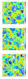 |
Fig. 1 Electron distribution (in log10 scale) in thesimulated Galactic midplane at 400 (top), 450 (middle), and 500 (bottom) Myr of disk evolution. |
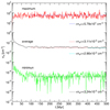 |
Fig. 2 Time evolution of the minimum (green), average (black), and maximum (red) electron density in the Galactic disk and time averages over 100–500 Myr (dashed black, red, and blue lines) and 400–500 Myr (cyan) of disk evolution are displayed. |
4.1 Volume analysis
Over time the population of electrons in the disk varies due to the different ongoing atomic and dynamical (including turbulent) processes. Therefore, the time evolution of their minimum, maximum, and averaged density in each region of the Galactic disk is not constant and can have large oscillations, as shown in Fig. 2, which displays the evolution of the minimum, maximum, and average density of the electrons in the simulated Galactic midplane over the 500 Myr of evolution. The time average of each plot is displayed with solid lines (for the average over the period 100–500 Myr). The time averages of the maximum is 57.9 cm−3, while the minimum time average is 3.24 × 10⁻⁵ cm−3. The averaged density over the 100–500 Myr period is 3.1 ×10⁻² cm−3 decreasing to 2.9 ×10⁻² cm−3 if the period 400–500 Myr is considered. We do not consider the first 100 Myr of disk evolution as it still reflects the initial conditions of the system (de Avillez & Breitschwerdt 2004).
The time evolution (100–500 Myr) of the volume occupation fraction of the free electrons enclosed in different temperature regimes (stable: T < 200 K, 103.9 < T ≤ 104.2 K, and T > 105.5 K; unstable: 200 < T ≤ 103.9 K and 104.2 < T ≤ 105.5 K) are shown in the top panel of Fig. 3. The different regimes have time averaged values of 3.8% (T <200 K), 50.8% (200 < T ≤ 103.9 K), 12.6% (103.9 < T ≤ 104.2 K), 14% (104.2 < T ≤ 105.5 K), and 18% for the hot gas (T > 105.5 K). The fraction of volume occupied by electrons that are locked in HI regions with densities higher than 1 and 0.3 cm−3 have a time averaged value of 5.8 and 7.6%, respectively, while electrons in the warm ionized medium (WIM, 6000 < T ≤ 104 K; Haffner et al. 2009) occupy 4.8% of the simulated disk volume. These values are similar to those discussed in de Avillez et al. (2012) and are in line with the observed values (Berkhuijsen et al. 2006; Berkhuijsen & Müller 2008; Gaensler et al. 2008). It is striking that more than 60% of the electrons are in classically thermally unstable regions.
Histograms of the electron distribution in the disk volume taken between 400 and 500 Myr with intervals of 20 Myr are shown in Fig. 4 (top panel). Although the histograms provide some information regarding the system at specific times, they are meaningful for the overall evolution of the free electrons in the ISM due to their variations, which are inherentto the underlying physical phenomena occurring at that time and captured in the corresponding histogram. These conditions may not repeat themselves at another time as the ISM is a nonlinear chaotic system. The spikes seen in the histograms are associated with the supernova activity, thus producing very hot gas (a few 107 K), in the disk leading to an increase in the number of electrons release by the different ions, most importantly from Si, S, and Fe. Nevertheless, these histograms suggest the presence of electrons with a Gaussian distribution centered at ≃ 3.0 × 10⁻² cm−3.
Moreover, we can see that the distribution of electrons (occupation fraction) becomes broader with time as successive supernova explosions drive the ISM, and hence electron density has more extreme values, i.e., denser regions become denser because of the compression of already compressed regions, and low density bubbles become less dense to due an increasing evacuation by each new explosion.
Even more information is provided by time averaged histograms (from 300 Myr through 500 Myr, using snapshots at every 1 Myr for a total of 51 snapshots) of the free electron distribution in the simulated disk (bottom panel of Fig. 4) for different temperature regimes (T ≤ 200 K, 200 < T ≤ 103.9 K, 103.9 < T ≤ 104.2 K, 104.2 < T ≤ 105.5 K, and T > 105.5 K) and total density. Although there are several differences among the averaged histogram profiles, they show that the total distribution (cyan line) of electrons is broad with a pronounced peak at around 3 × 10⁻² cm−3 and are dominated by the thermally unstable gas at 200 < T ≤ 103.9 K (totally unstable) centered at 4 × 10⁻² cm−3 and 104.2 < T ≤ 105.5 K (partially unstable) for densities greater than 3 × 10⁻³ cm−3. It also includes the contributions of the thermally stable regimes (T ≤ 200 K and 103.9 < T ≤ 104.2 K) at the level of few percent level. The cold gas below 200 K only harbors a very small fraction of electrons. At lower densities the total distribution is defined by the hot gas (T > 105.5) and by the thermally unstable gas with 105.0 < T ≤ 105.5 K. It is not surprising that the hot gas at T > 105.5 K, which has a large number of free electrons, contributes substantially to the total histogram at lower densities.
The time averaged histograms are fitted with a composition of two Gaussian distributions with mean values of ne = 4.1 × 10⁻⁴ cm−3 determined by the hot gas and ne = 2.9 × 10⁻²− 3.1 × 10⁻² cm−3 for the right Gaussian distributions. The mean electron density is in line with the value measured in the simulated disk, as discussed above (see Fig. 2).
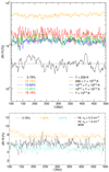 |
Fig. 3 Time evolution of the occupation fractions (percent of the disk volume) of the electrons associated with the different temperatureregimes (top panel) and in HI regions and in the warm ionized medium (bottom panel). |
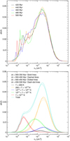 |
Fig. 4 Top panel: histograms of the electron density in the Galactic disk at different times from 400 through 500 Myr at every 20 Myr. Bottom panel: time averaged volume histograms of the electron density in the Galactic disk for different temperature regimes and total density (brown) calculated between 400 and 500 Myr using 51 snapshots with a time interval of 1 Myr. |
4.2 Line of sight observations
Using three vantage points (A, B, C) in the simulated Galactic midplane located at A (x = 0, y = 0, z = 0) pc, B (x = 1000, y = 0, z = 0), and C (x = 1000, y = 500, z = 0), LOS measurements were taken at distances of up to 4000 pc from the observer. The lines of sight span a projected area (onto the simulated Galactic midplane) with an angle of 80° from locations A (ranging from 0° to 80°; green lines) and B (ranging from 95° to 175°; red lines) and 90° from location C (ranging from 135° to 225°; blue lines) at every 2°. Thus, a total of 41 (from locations A and B) and 46 (from location C) lines of sight were taken.
Figure 5 displays the vantage point locations and the projected areas onto the simulated Galactic midplane covered by the lines of sight taken from those locations and extending to 2 kpc. The measurements through distances longer than the linear side of the section of the simulated disk, shown in the figure by the square with black solid lines, takes advantage of the periodic boundary conditions adopted along the computational domain faces perpendicular to the Galactic midplane, thus adding up the data cubes as needed in the x and y directions, as shown in the figure by the dotted squares.
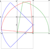 |
Fig. 5 Vantage points and areas projected onto the simulated Galactic midplane of 80° and 90° covered by the lines of sight taken from locations A, B, and C and extending over 2 kpc. The computational domain is represented by the solid black lines, while the replicated domains are represented by dotted lines. |
4.2.1 Dispersion measures
The dispersion measures observed from the different vantage points vary between lines of sight and along lines of sight, as can be seen in Fig. 6, which displays the angular distribution of the electrons column density measured at 300 (top), 400 (middle), and 500 (bottom panel) Myr from the vantage points A (black lines), B (green lines), and C (red lines) for LOS with lengths 4000, 3000, 2000, 1000, 500, 100, and 10 (from top to bottom). For the sake of clarity the DMs from position C are deviated 25° from their original angles (135°−225°) in order to avoid overlap with the observations from position B.
The LOSs trace the underlying topology of the interstellar gas as the lines cross regions with very different electron densities. Thus, regions with very low density (e.g., bubbles or supperbubbles) do not contribute much to the DM, and this is reflected in the dips seen in the angular distribution. Similarly, the presence of a shell or a cloud leads to an increase in the column density, hence a sudden increase in the DM, as can be seen in the figure. The largest variations in the dispersion measures at each position and between the different positions occur for lLOS = 10 and 100 pc. The gap between the DMs at these distances varies between positions and in time (compare the two bottom lines for each position in each panel of Fig. 6). The dispersion measures for lLOS ≥ 500 pc although varying over the angles, their positions in the different panels are similar between the three vantage points. We note that this distance is six times the correlation length (75 pc) measured in the simulated ISM, thus a repetition pattern in the ISM occurs for a few correlation lengths (see, e.g., de Avillez & Breitschwerdt 2007), which is imprinted in the spatial distribution of the DMs for larger LOS lengths.
Due to the variability of the topology of the turbulent ISM as a result of the ongoing processes the DMs observed at a specific time, because of their large variation among and along lines of sight, as can be seen in Fig. 6, are not representative of the system evolution overall. A more adequate indicator is the time average of the DMs combining different sets of data cubes spanning an evolutionperiod of ISM. Figure 7 displays the minimum, average, and maximum of the time averaged DMs,  1 (cm−3 pc), determined up to 4 kpc from the vantage points A, B, and C over 11, 51, and 101 data cubes with time intervals of 1 Myr (in the ranges 300–310, 400–450 and 450–50, and 400–500 Myr). The figure also displays the dispersion measures obtained against pulsars of known distance located up to 200 pc above and below the Galactic midplane and taken from de Avillez et al. (2012) and Yao et al. (2017).
After an initial steep rise in the vicinity of the vantage point (for LOS up to 300 pc) the dispersion measures show a linear growth with distance (with average values of 25–35 and 105–120 cm−3 pc at 1000 and 4000 pc, respectively; see Table 1) with an average increase of 27 cm−3 pc per kpc in the DM. In addition, there is an almost constant dispersion (with distance) with regard to the average of  over 11, 51, and 101 Myr averages.
With the increase in the number of data cubes used in the averaging process the smoothness in the curves increases (compare the evolution of the DM curves in all the plots) in particular for the LOS lengths smaller than 1 kpc. For larger LOSs the curves show a systematic smoothness. However, although the averaging process smooths out the larger variations on the electron distribution in the simulated ISM, the 50 and 100 Myr averages still have the imprint of the underlying interstellar gas topology mostly resulting from long-lasting structures such as superbubbles that exist for tens of millions of years. Consequently, even with these longer averaging periods there is variability in the dispersion measures and in the mean electron density among the lines of sight and for the different vantage points.
Overall the DMs, and the derived mean electron density, in the simulated disk are in line with the DMs obtained against pulsars of know distances with the maximum and minimum values of the DMs being in the interval defined by the observations.
The constancy of the time averaged dispersion measures with regard to the average shown in Fig. 7 is indicative of the spatial organization of the electrons in the ISM (see similar discussion, which we follow, in the context of OVI observationsin Bowen et al. 2008). If the LOSs intercept clouds of electrons with a fixed dispersion measure (e.g., DM°), then the total DM resulting from the interception of N clouds would be N DM° with a dispersion varying as  . Hence, the dispersion should decrease with distance and approach the observed DM as the number of clouds increases and their DM decreases (Fig. 8). This reduction in the dispersion is not observed in Fig. 7. The observed clumpiness results from the fact that SNe increase the number and especially the density of shock compressed layers, and evacuate bubbles, so that the electron density becomes very inhomogeneous with time.
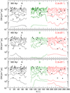 |
Fig. 6 Angular distribution of the dispersion measures observed from positions A, B, and C at (from top to bottom) 4000, 3000, 2000, 1000, 500, 100, and 10 pc. The data from position C is deviated by 25° with regard to their original angles (135°−225°) in order to avoid overlapping with the observations between positions B and C. |
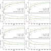 |
Fig. 7 Time averaged dispersion measures ( |


4.2.2 Mean electron density
The averaged observations from each vantage point in the simulated disk show a variability in the dispersion measures, and therefore, inthe derived mean electron density; see bottom of each panel in Fig. 7, which displays the minimum, maximum, and average electron density with distance derived from the time averaged dispersion measures (i.e., 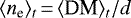 (cm−3)). The average of the derived mean electron density is denoted
  .
.
In the first 200 pc from the vantage points the average  increases to a maximum that varies among the different vantage points, the largest being 8 × 10⁻² cm−3 at position C for 450–500 Myr averages. After this initial rise in
  there is a stabilization with distance towards the values measured for a LOS length of 4 kpc and displayed in Table 1. These densities not only vary between vantage points, but also according to the averaging period, and have a value between 2.64 × 10⁻² and 3 × 10⁻² cm−3, a variation of 13.6% with regard to the lowest value in the 7th column of the table.
The averaging process did not provide a common value for the three vantage points other than smoothing their distance variations as the number of data cubes increases from 11 to 51 and 101. The electron density in the Galactic midplane varies between the vantage points for each averaging period, and can be as high as 6% for the 300–310 Myr, 8.33% for the 400–450 Myr, 2.9% for the 450–500 Myr, and 5.5% for the 400–500 Myr period average.
It should be pointed out that these values are consistent with the mean values derived from the averaged electron density PDFs obtained along the lines of sight and with the average electron density obtained through the volume analysis displayed in Fig. 2.
Averages of the time averaged dispersion measures ( ) and derived mean electron density
  ), calculated in 300–310, 400–450, 450–500, 400–500 Myr, for line of sight lengths of 1, 2, 3, and 4 kpc, and taken from the vantage points (VP) A, B, and C.
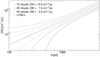 |
Fig. 8 Variation in the dispersion with distance as the LOSs cross 10, 20, and 40 clouds with DM of 14 (blue), 7 (red), and 3.5 (green) cm−3 pc. |
5 Discussion and final remarks
In this work we recalculated the electron distribution in the ISM using self-consistent three-dimensional time-dependent dynamical and ionic calculations of the interstellar gas composed of atoms, ions, and electrons due to the ten most abundant elements in nature. The calculations include, among other processes, charge transfer reactions, radiative and dielectronic recombination, electron impact ionization, excitation-auto ionization, and photoionization.
These calculations differ from the previous work of de Avillez et al. (2012) in the following ways: (i) inclusion of photoionization due to the interstellar radiation field (in addition to the other physical processes used in that work); (ii) inclusion of secondary electrons; (iii) calculation of the line emission using 30 levels per atom or ion, using up-to-date collision strengths (de Avillez et al. 2018); and (iv) update of rates associated with radiative and dielectronic recombination and charge-transfer. Therefore, the thermal evolution in the two simulations should show differences, for example in (1) the line emission (the level populations are better constrained than in the previous simulation where transitions to the ground state were assumed), (2) the emission due to the other processes as a result of updated rates, and (3) the ionic evolution of the plasma as a result of updated atomic data and the inclusion of photoionization. The last is responsible for the injection of photo-electrons, which in turn interact with other electrons and ions until their energy is degraded and deposited as heat in the medium (see, e.g., Shull 1979; Furlanetto & Stoever 2010). The extent of these differences and how they affect the simulations, and in particular the electron distribution in the interstellar gas, is the subject of a forthcoming paper.
From the volume and LOS analysis it turns out that the mean electron density in the Galactic midplane depends on the methods used. The volume analysis shows a mean electron density of ≃ 0.03 cm−3, while the LOS observations point to average values in therange 0.026–0.029 cm−3 and 0.027–0.029 cm−3 for averagedperiods of 50 and 100 Myr, respectively. These values, although their differences are small, depend on the location of the vantage point.
The volume averaging includes the whole volume which tends to reduce the mean value, while the LOS average depends on the lines crossing the disk, and thus a fraction of the volume is missed. Hence, the averaged density obtained with the LOS can vary. Therefore, this selection effect should be taken into consideration when deriving the mean electron density. Theresults for the electron density in the Galactic midplane are in line with that obtained by Gaensler et al. (2008), Berkhuijsen & Fletcher (2008), Schnitzeler (2012), and Yao et al. (2017), among others, and are 22.5% lower than the electron density in the Galactic midplane obtained by de Avillez et al. (2012).
As we found previously, the largest contributor to ne comes from a thermally unstable phases of the ISM, with temperatures between 200 and 103.9 K and between 104.2and 105.5 K, instead of the classical warm ISM with temperatures between 103.9and104.2 K. The hot phase of the ISM has a very low free electron density of 4.1 × 10⁻⁴ cm−3, while the combination of all other ISM phases has an average free electron density of about 0.03 cm−3.
Dispersion measures show large variations over time if sightlines are short (≲ 100 pc). Over longer distances, the fluctuations become smaller through averaging. The ratio of the DM variation (of all points at a certain distance along the line of sight) to the average DM (of those points) does not decrease, which is caused by the many evacuated bubbles and shock compressed layers in the Galactic ISM. In a toy model where a line of sight intersects clouds of constant electron density, and where the number density of clouds is the same along the line of sight, the ratio of the DM fluctuations to DM decreases for longer lines of sight, which does not match the results of our simulations.
Acknowledgements
This research was supported by the projects “Hybrid computing using accelerators & coprocessors - modelling nature with a novell approach” (PI: M.A.), InAlentejo program, CCDRA, Portugal, and “Enabling Green E-science for the SKA Research Infrastructure (ENGAGE SKA)”, reference POCI-01-0145-FEDER-022217, funded by COMPETE 2020 and Foundation for Science and Technology (FCT), Portugal. The calculations were carried out at the Xeon Phi Orion cluster (Computational Astrophysics Group), while the data analytics was performed at the OBLIVION Supercomputer (ENGAGE SKA), both machines based at the University of Évora.
References
- Amarsi, A. M., & Asplund, M. 2017, MNRAS, 464, 264 [NASA ADS] [CrossRef] [Google Scholar]
- Asplund, M., Grevesse, N., Sauval, A. J., & Scott, P. 2009, ARA&A, 47, 481 [NASA ADS] [CrossRef] [Google Scholar]
- Berkhuijsen, E. M., & Fletcher, A. 2008, MNRAS, 390, L19 [NASA ADS] [CrossRef] [Google Scholar]
- Berkhuijsen, E. M., & Müller, P. 2008, A&A, 490, 179 [NASA ADS] [CrossRef] [EDP Sciences] [Google Scholar]
- Berkhuijsen, E. M., Mitra, D., & Mueller, P. 2006, Astron. Nachr., 327, 82 [NASA ADS] [CrossRef] [Google Scholar]
- Bowen, D. V., Jenkins, E. B., Tripp, T. M., et al. 2008, ApJS, 176, 59 [NASA ADS] [CrossRef] [Google Scholar]
- Cordes, J. M., & Lazio, T. J. W. 2002, ArXiv e-prints [astro-ph/0207156] [Google Scholar]
- Cordes, J. M. & Lazio, T. J. W. 2003, ArXiv e-prints [astro-ph/0301598] [Google Scholar]
- Davidson, P. A. 2004, Turbulence: An Introduction for Scientists and Engineers (Orford: Oxford University Press) [Google Scholar]
- de Avillez M. 2018, Cosmic Rays and the InterStellar Medium, 28 [Google Scholar]
- de Avillez, M. A., & Breitschwerdt, D. 2004, A&A, 425, 899 [NASA ADS] [CrossRef] [EDP Sciences] [Google Scholar]
- de Avillez, M. A., & Breitschwerdt, D. 2007, ApJ, 665, L35 [NASA ADS] [CrossRef] [Google Scholar]
- de Avillez, M. A. & Breitschwerdt, D. 2010, ASP Conf. Ser., 438, 313 [Google Scholar]
- de Avillez, M. A., & Breitschwerdt, D. 2012a, ApJ, 761, L19 [NASA ADS] [CrossRef] [Google Scholar]
- de Avillez, M. A., & Breitschwerdt, D. 2012b, ApJ, 756, L3 [NASA ADS] [CrossRef] [Google Scholar]
- de Avillez, M. A., & Mac Low M.-M. 2002, ApJ, 581, 1047 [NASA ADS] [CrossRef] [Google Scholar]
- de Avillez, M. A., Asgekar, A., Breitschwerdt, D., & Spitoni, E. 2012, MNRAS, 423, L107 [CrossRef] [Google Scholar]
- de Avillez, M. A., Anela, G. J., & Breitschwerdt, D. 2018, A&A, 616, A58 [NASA ADS] [CrossRef] [EDP Sciences] [Google Scholar]
- Elmegreen, B. G., & Scalo, J. 2004, ARA&A, 42, 211 [NASA ADS] [CrossRef] [Google Scholar]
- Ferrière, K. M. 2001, Rev. Mod. Phys., 73, 1031 [NASA ADS] [CrossRef] [Google Scholar]
- Furlanetto, S. R., & Stoever, S. J. 2010, MNRAS, 404, 1869 [NASA ADS] [Google Scholar]
- Gaensler, B. M., Madsen, G. J., Chatterjee, S., & Mao, S. A. 2008, PASA, 25, 184 [NASA ADS] [CrossRef] [Google Scholar]
- Habing, H. J. 1968, Bull. Astron. Inst. Netherlands, 19, 421 [Google Scholar]
- Haffner, L. M., Dettmar, R.-J., Beckman, J. E., et al. 2009, Rev. Mod. Phys., 81, 969 [NASA ADS] [CrossRef] [Google Scholar]
- Helmi, A. 2004, MNRAS, 351, 643 [NASA ADS] [CrossRef] [Google Scholar]
- Jiang, R. L., Fang, C., & Chen, P. F. 2012, Comput. Phys. Commun., 183, 1617 [CrossRef] [Google Scholar]
- Joung, M. R., Bryan, G. L., & Putman, M. E. 2012, ApJ, 745, 148 [NASA ADS] [CrossRef] [Google Scholar]
- Kuijken, K., & Gilmore, G. 1989, MNRAS, 239, 651 [NASA ADS] [Google Scholar]
- Pradhan, A. K., & Nahar, S. N. 2011, Atomic Astrophysics and Spectroscopy (Cambridge: Cambridge University Press) [CrossRef] [Google Scholar]
- Schnitzeler, D. H. F. M. 2012, MNRAS, 427, 664 [NASA ADS] [CrossRef] [Google Scholar]
- Scott, P., Asplund, M., Grevesse, N., Bergemann, M., & Sauval, A. J. 2015a, A&A, 573, A26 [NASA ADS] [CrossRef] [EDP Sciences] [Google Scholar]
- Scott, P., Grevesse, N., Asplund, M., et al. 2015b, A&A, 573, A25 [NASA ADS] [CrossRef] [EDP Sciences] [Google Scholar]
- Shull, J. M. 1979, ApJ, 234, 761 [NASA ADS] [CrossRef] [Google Scholar]
- Slavin, J. D., & Cox, D. P. 1992, ApJ, 392, 131 [NASA ADS] [CrossRef] [Google Scholar]
- Verner, D. A., & Yakovlev, D. G. 1995, A&AS, 109, 125 [NASA ADS] [Google Scholar]
- Verner, D. A., Ferland, G. J., Korista, K. T., & Yakovlev, D. G. 1996, ApJ, 465, 487 [Google Scholar]
- Wolfire, M. G., Hollenbach, D., McKee, C. F., Tielens, A. G. G. M., & Bakes, E. L. O. 1995, ApJ, 443, 152 [Google Scholar]
- Yao, J. M., Manchester, R. N., & Wang, N. 2017, ApJ, 835, 29 [NASA ADS] [CrossRef] [Google Scholar]

All Tables
Averages of the time averaged dispersion measures () and derived mean electron density ), calculated in 300–310, 400–450, 450–500, 400–500 Myr, for line of sight lengths of 1, 2, 3, and 4 kpc, and taken from the vantage points (VP) A, B, and C.
All Figures
|
Fig. 1 Electron distribution (in log10 scale) in thesimulated Galactic midplane at 400 (top), 450 (middle), and 500 (bottom) Myr of disk evolution. |
| In the text | |
|
Fig. 2 Time evolution of the minimum (green), average (black), and maximum (red) electron density in the Galactic disk and time averages over 100–500 Myr (dashed black, red, and blue lines) and 400–500 Myr (cyan) of disk evolution are displayed. |
| In the text | |
|
Fig. 3 Time evolution of the occupation fractions (percent of the disk volume) of the electrons associated with the different temperatureregimes (top panel) and in HI regions and in the warm ionized medium (bottom panel). |
| In the text | |
|
Fig. 4 Top panel: histograms of the electron density in the Galactic disk at different times from 400 through 500 Myr at every 20 Myr. Bottom panel: time averaged volume histograms of the electron density in the Galactic disk for different temperature regimes and total density (brown) calculated between 400 and 500 Myr using 51 snapshots with a time interval of 1 Myr. |
| In the text | |
|
Fig. 5 Vantage points and areas projected onto the simulated Galactic midplane of 80° and 90° covered by the lines of sight taken from locations A, B, and C and extending over 2 kpc. The computational domain is represented by the solid black lines, while the replicated domains are represented by dotted lines. |
| In the text | |
|
Fig. 6 Angular distribution of the dispersion measures observed from positions A, B, and C at (from top to bottom) 4000, 3000, 2000, 1000, 500, 100, and 10 pc. The data from position C is deviated by 25° with regard to their original angles (135°−225°) in order to avoid overlapping with the observations between positions B and C. |
| In the text | |
|
Fig. 7 Time averaged dispersion measures ( |
| In the text | |
|
Fig. 8 Variation in the dispersion with distance as the LOSs cross 10, 20, and 40 clouds with DM of 14 (blue), 7 (red), and 3.5 (green) cm−3 pc. |
| In the text | |
Current usage metrics show cumulative count of Article Views (full-text article views including HTML views, PDF and ePub downloads, according to the available data) and Abstracts Views on Vision4Press platform.
Data correspond to usage on the plateform after 2015. The current usage metrics is available 48-96 hours after online publication and is updated daily on week days.
Initial download of the metrics may take a while.