| Issue |
A&A
Volume 644, December 2020
|
|
|---|---|---|
| Article Number | A28 | |
| Number of page(s) | 7 | |
| Section | The Sun and the Heliosphere | |
| DOI | https://doi.org/10.1051/0004-6361/202038925 | |
| Published online | 25 November 2020 | |
Exploring the coronal evolution of AR 12473 using time-dependent, data-driven magnetofrictional modelling⋆
Department of Physics, University of Helsinki, Helsinki, Finland
e-mail: This email address is being protected from spambots. You need JavaScript enabled to view it.
Received:
14
July
2020
Accepted:
2
October
2020
Abstract
Aims. We present a detailed examination of the magnetic evolution of AR 12473 using time-dependent, data-driven magnetofrictional modelling.
Methods. We used maps of the photospheric electric field inverted from vector magnetogram observations, obtained by the Helioseismic and Magnetic Imager onboard the Solar Dynamics Observatory (SDO), to drive our fully time-dependent, data-driven magnetofrictional model. Our modelled field was directly compared to extreme ultraviolet observations from the Atmospheric Imaging Assembly, also onboard SDO. Metrics were also computed to provide a quantitative analysis of the evolution of the magnetic field.
Results. The flux rope associated with the eruption on 28 December 2015 from AR 12473 was reproduced by the simulation and found to have erupted due to a torus instability.
Key words: Sun: coronal mass ejections (CMEs) / Sun: corona / magnetic fields / magnetic reconnection / methods: numerical / methods: data analysis
Movies associated with Figs. 1 and 5 are available at https://www.aanda.org
© ESO 2020
1. Introduction
Coronal mass ejections (CMEs; for a review see e.g. Slemzin et al. 2019) are huge eruptions of plasma and magnetic field ejected from the Sun that drastically affect conditions in the heliosphere. It is now generally accepted that CMEs form as twisted and helical magnetic field structures, known as flux ropes, whose eruptions are driven by the release of free magnetic energy that has accumulated in the corona (e.g. Vourlidas et al. 2017; Green et al. 2018). The formation of flux ropes in the corona and the detailed mechanisms by which they lose stability and are ejected from the Sun stand as open research questions (e.g. Welsch 2018). A detailed knowledge of the magnetic field and its dynamical evolution in the corona is crucial for supporting these efforts. The magnetic field is also a critical piece of information for predicting the consequences of CMEs in terms of space weather when they are aligned with the Earth (e.g. Schwenn 2006; Kilpua et al. 2017; Eastwood et al. 2018; Kilpua et al. 2019).
It is, however, difficult to measure the magnetic field directly in the corona. The coronal loops can be viewed in extreme ultraviolet (EUV) images due to the emitting plasma tracing them out, but these observations are subject to a host of visualisation effects. In addition, there are often not enough perspectives available to create a true picture, nor do existing ones directly provide information on the magnetic field magnitude and direction. Consequently, modelling of the coronal field is necessary for achieving a better understanding of the evolution of coronal structures. Observations of the photospheric magnetic field, on the other hand, are continuously available and can be utilised as boundary conditions for extrapolating and modelling the magnetic field in the corona (e.g. Wiegelmann & Sakurai 2012).
One such data-driven approach is magnetofrictional modelling (MFM, Yang et al. 1986), which assumes that magnetic forces dominate in the corona and that thermodynamics can be neglected because of the low plasma beta of the active corona. This assumption is implemented via a friction term that is included into the MHD (magnetohydrodynamics) momentum equation and the system attempts to evolve towards a force-free state. If the photospheric boundary conditions are evolved in time, the force-free state is not reached (e.g. van Ballegooijen et al. 2000) and MFM can be used to create fully time-dependent data-driven simulations of coronal evolution. A range of authors have demonstrated the capacity of such simulations to model solar eruptions (e.g. Cheung & DeRosa 2012; Cheung et al. 2015; Fisher et al. 2015; Yardley et al. 2018; Pomoell et al. 2019; Price et al. 2019). Most of these studies have also emphasised the importance of a complete constraining of the driving photospheric electric field, showing that the non-inductive electric field component is crucial for capturing the complex dynamics of the coronal magnetic field. Price et al. (2019) was particularly focused on the structure and formation of the flux rope and demonstrated that with an accurate estimation of the electric field the magnetofrictional simulation successfully produced magnetic field evolution that is consistent with observations of the active region under study. Here, we instead focus on probing the stability of a flux rope that forms self-consistently in the simulation to determine how and why it erupted, thereby demonstrating the capacity of magnetofrictional simulations to capture essential eruption dynamics.
In this paper, we perform a time-dependent and data-driven magnetofrictional simulation of NOAA Active Region (AR) 12473 to model the flux rope related to a CME that erupted from this AR on 28 December 2015. The driving electric field is constrained using an ad-hoc assumption for the non-inductive component of the electric field. Our data-driven simulation forms a clear flux rope that goes on to exit through the upper boundary of the simulation domain. We also explore the structure of the flux rope and the mechanism leading to its destabilisation, for instance, by analysing the rate of decay of the overlying magnetic field in conjunction with the relaxation runs. The paper is organised as follows. In Sect. 2, we summarise the data and the simulation method that we used. In Sect. 3, we analyse and interpret the simulation results. Finally, in Sect. 4, we present our conclusions.
2. Data and methods
This study targets the eruption that occurred from AR 12473 at approximately 11:30 UT on 28 December 2015. At this time, the AR was located close to the disk centre as viewed from Earth in the southern hemisphere (S22W18). The eruption resulted in a CME that was classified as a full halo from the Earth’s perspective in the CME catalogue1 of the LASCO coronagraph (Brueckner et al. 1995) onboard the SOHO spaceraft (Domingo et al. 1995). The first observation of the CME in the LASCO/C2 field of view was at 12:12 UT on 28 December and it was fast, with its linear speed reported to be 1212 km s−1. The eruption was associated with a M1.9 flare that started at 11:20 UT (peak at 12:45 UT) on the same day and coming from the same active region. A few days later, an interplanetary CME (ICME) in the near-Earth solar wind with a flux rope structure (Lepping et al. 1995) and an intense geomagnetic storm was reported. For example, the online Richardson and Cane ICME catalogue2 marks the shock ahead of the ICME at 00:50 UT and the ICME leading edge at 17:00 UT on 31 December. Here, we focus on the modelling of the eruption in the corona. However, given the clear in situ counterpart and a significant geomagnetic storm, this event is suitable for future studies focussed on assessing the ability of the model to predict the magnetic structure of the CME in the heliosphere.
2.1. Data
For the lower boundary condition to our data-driven coronal simulation (Pomoell et al. 2019), we used photospheric vector magnetogram observations provided by the Helioseismic and Magnetic Imager (HMI; Scherrer et al. 2012) onboard the Solar Dynamics Observatory (SDO; Pesnell et al. 2012). The magnetograms (HMI data product hmi.B_720s) were downloaded in their native 0.5″ spatial resolution with a 720 s cadence. They were then processed for the simulation using the pipeline described in Lumme et al. (2017) and Pomoell et al. (2019), as detailed in Sect. 2.1 of Price et al. (2019). A brief summary of the processing steps is as follows. Firstly, bad pixels and spurious temporal flips in the azimuth were removed and data gaps linearly interpolated. The magnetograms were then temporally and spatially smoothed, and rebinned to four times lower spatial resolution. Finally, the magnetic field was made to smoothly approach zero at the boundaries and the magnetograms were flux-balanced using a multiplicative method.
We compare the simulation results to coronal extreme ultraviolet observations taken by the Atmospheric Imaging Assembly (AIA; Lemen et al. 2012), also onboard SDO. The flare and CME were most clearly depicted by the 193 Å channel shown in Fig. 1. There are a number of rising loop-like structures approximately in the direction indicated by the arrows, followed by a large, very clear, set of post-eruption arcades. However, as the basis of the comparison to our simulation results, we selected the 94 Å channel due to its higher characteristic temperature, which is associated with flaring structures (i.e. it has the clearest depiction due to the emission from the hot plasma filling the magnetic field lines of the flux rope).
 |
Fig. 1. Series of AIA 193 Å observations depicting structures prior to the flare (left), shortly after the flare (middle), and four hours following the flare (right) that took place at approximately 11:20 UT. This figure is available as an online movie in the 94 Å and 193 Å channels. |
2.2. Methods
2.2.1. Electric field inversion
The HMI vector magnetogram data were processed and used to generate a time series of electric fields for the simulations using the ELECTRIC field Inversion Toolkit (ELECTRICIT; Lumme et al. 2017) in a manner consistent with the description from Price et al. (2019). At its core, this method decomposes the electric field into its inductive, EI, and non-inductive, −∇ψ, components as E = EI − ∇ψ. The inductive component is simply calculated from Faraday’s law. However, additional observables, such as photospheric velocity estimates, would be needed to determine the non-inductive components (Fisher et al. 2010; Kazachenko et al. 2014). Therefore, as in our previous studies (see e.g. Lumme et al. 2017; Pomoell et al. 2019; Price et al. 2019), we approximate the non-inductive component of the electric field using an optimisation approach in which a particular functional form for the non-inductive component is assumed a priori. The “U assumption” from Cheung et al. (2015) defines the non-inductive component as follows:
 (1)
(1)
where U is a free parameter with units of velocity and in a highly idealised situation corresponds to the vertical emergence velocity of a twisted magnetic flux tube through the photosphere (see Lumme et al. 2017, for details).
To find the optimal value of U, under the assumption that it is a constant both temporally and spatially, we minimised the root mean square error between the total photospheric energy injection (the vertical Poynting flux integrated over time and area) of the electric fields computed using a given U and a reference estimate calculated using DAVE4VM (Differential Affine Velocity Estimator for Vector Magnetograms; Schuck 2008). This electric field inversion process was carried out while the centre of the AR was within 50 degrees from the central meridian in order to reduce the impact of data quality degradation close to the limb (Sun & Norton 2017). Consequently, and for the same reason, all coronal simulations began while the AR was within ∼50 degrees of the central meridian. This resulted in the AR having already emerged by the start of the simulation time, although it had already partially emerged when it appeared at the limb. We note that while previous studies (see e.g. Kazachenko et al. 2014; Lumme et al. 2017; Pomoell et al. 2019; Price et al. 2019) had the magnetograms masked such that pixels for which the total field was below a given threshold were set to zero, in our study, no masking was applied. Omitting the masking was, in this case, found to result in a slightly better agreement with DAVE4VM in terms of the injection of photospheric relative helicity. The coronal evolution was found to be very similar in both cases, so henceforth we discuss only the unmasked case.
2.2.2. Magnetofrictional modelling
We carried out magnetofrictional simulations using the time-dependent, data-driven model described in Pomoell et al. (2019). The resistivity was uniform throughout the domain and held constant at 200 × 106 m2 s−1. The frictional coefficient was similarly constant at 1 × 10⁻¹¹ s m−2, except close to the lower boundary where our velocity smoothly approaches zero. The top and the side boundaries of the domain were open and the simulation was initialised with a potential field. The input magnetogram and electrograms were padded with a border of 25 pixels of zeroes to minimise boundary effects and the coronal domain was chosen to have a height of 200 Mm. The simulation was carried out from 23:24 UT on 23 December until approximately when the AR reached the western limb at 16:36 UT on 02 January.
3. Results and discussion
In this section, we analyse and interpret the results of our time-dependent, data-driven simulation using a combination of metrics and relaxation simulations.
3.1. Injection of Poynting flux and helicity
Initially, we set out to investigate the photospheric Poynting flux and helicity injections. Figure 2 depicts the temporal evolution of the photospheric energy injection for the electric field inverted using the optimal value U = 120 ms−1, as obtained in Sect. 2.2.1 (blue curve), and the reference DAVE4VM values (orange curve). We attribute the minor periodic variations in the U curve to the 24 h orbital period of SDO. The AR is within 50 degrees of the disk centre for the period shown. We find good agreement between the two curves, although the U curve begins to increasingly overestimate the injected Poynting flux as it approaches the 50 degree limit.
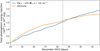 |
Fig. 2. Temporal evolution of the photospheric energy injection for AR 12473. Displayed: optimised U (blue) and reference DAVE4VM (orange) totals. The vertical dotted line indicates the time of the M1.9 flare. |
Even though only the energy injection was used to determine the optimal value of U, due to the importance of helicity in solar eruptions (Pomoell et al. 2019; Price et al. 2019) the total photospheric relative helicity injection was similarly integrated in time and space, as shown by Fig. 3. The U (blue) and DAVE4VM (orange) curves are initially in very good agreement. However, they begin to diverge approximately 24 h from the start of the time series, resulting in the U electric fields increasingly overestimating the injected helicity when compared to DAVE4VM. While Price et al. (2019) used a different assumption for the non-inductive component of the electric field, their final electric fields overestimated the injected helicity by a similar amount. As noted in Sect. 2.2.1, our decision to not mask the magnetograms was guided by the helicity injection. Masking resulted in an increased overestimation of the helicity injection, for example, when the mask was set to 250 G, the injection was ∼19% greater than in the unmasked case at the time of the flare. The issue of how masking can affect an active region is discussed in detail by Lumme et al. (2017).
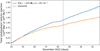 |
Fig. 3. Temporal evolution of the photospheric relative helicity injection for AR 12473. Displayed: optimised U (blue) and reference DAVE4VM (orange) totals. The vertical dotted line indicates the time of the M1.9 flare. |
3.2. Evolution of magnetic energy and helicity in the corona
To quantitatively examine the coronal evolution, we computed the total magnetic energy, εM, and the free magnetic energy, εfree, contained in the coronal domain as below:
 (2)
(2)
 (3)
(3)
where B denotes the magnetic field, Bp the potential field, and μ0 the permeability of free space or the magnetic constant. These metrics are displayed by Fig. 4a, along with the ratio of free to total magnetic energy for the period when the AR was within 50 degrees of the disk centre. Despite the fluctuations, it is clear that there is an initial increase in total magnetic energy, peaking at approximately 00:00 UT on 25 December, followed by a subsequent decrease, reaching a minimum at approximately 12:00 UT on 27 December. This decrease coincides approximately with the formation of the flux rope along with flux cancellation at the photosphere. Flux rope formation has been related to flux cancellation in some studies (e.g. Green et al. 2011). However, the subsequent increase in total magnetic energy coincides with further flux emergence suggesting the previous decrease may primarily be due to the cancellation.
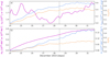 |
Fig. 4. Temporal evolution of volume metrics showing (a) the free magnetic energy (blue), magnetic energy (purple), and the ratio of the free to the total magnetic energy (orange); and (b) the current-carrying helicity (blue), relative helicity (purple), and the ratio of the current-carrying to the relative helicity (orange) for AR 12473. The vertical dotted line indicates the time of the M1.9 flare. |
In contrast to the total magnetic energy, the free magnetic energy (blue curve) increases approximately steadily from the start of the simulation until approximately 00:00 UT on 30 December. There is, however, a notable saturation at approximately 12:00 UT on 27 December, coinciding with the minimum in magnetic energy described above before resuming its rise at approximately 06:00 on 28 December. The ratio of the free magnetic energy to the total magnetic energy largely follows the behaviour of the free magnetic energy.
In addition, we calculated the relative helicity, HR, contained in the coronal volume and decomposed it, as in Berger (2003), to get the current-carrying helicity, Hj, as follows:
 (4)
(4)
 (5)
(5)
 (6)
(6)
where A denotes the vector potential of the magnetic field B and Ap denotes the vector potential of the potential magnetic field Bp, with Hpj as the mutual helicity between the current-carrying and the potential field. These metrics are shown in Fig. 4b alongside the ratio of the current-carrying to the relative helicity. Both the relative helicity (purple curve) and the current-carrying helicity (blue curve) increase over the simulation time until approximately 00:00 UT on 31 December. The constantly increasing helicity is expected due to the constant photospheric driving introducing helicity into the domain, as shown in Fig. 3. We note that the rate of increase of current-carrying helicity clearly increases at approximately 00:00 UT on 25 December, coinciding with the initial peak in magnetic energy and the forming of the flux rope.
3.3. Evolution of the magnetic field topology
Next, we investigated the evolution of the structure of the magnetic field in the corona. We computed the twist number, Tw, using the open-source software of Liu et al. (2016). Tw measures the turns of two infinitesimally close magnetic field lines about each other. It was considered because a flux rope is expected to have a consistent sign of Tw and a magnitude greater than one.
Plots of the magnetic field lines are shown for every 24 hours in Fig. 5, including a vertical plane and contours of Tw in the first row and an unobstructed view of the field lines in the second row. The flux rope field lines trace a region of the flux rope for which Tw > 1.5 (cyan contour). Thus, the plots here do not show the full extent of the flux rope because its cross-section, by definition, encompasses the larger region where Tw > 1.0 (dark blue contour). We however decided to show the smaller area for the sake of a clearer depiction as it is more well defined. The Tw > 1.0 and the Tw > 1.5 contours are not regular circles, especially the Tw > 1.0 contour, but they are very coherent. The temporal evolution of the Tw and Bz planes from Fig. 5 are available as online movies.
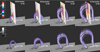 |
Fig. 5. Simulation excerpts from 11:36 UT on 28 December to 11:36 UT on 31 December with a spacing of 24 h between each image. Top row: flux rope for field lines where Tw > 1.5. It is bisected by a plane of Tw that also plots the contours of Tw. Bottom row: unobstructed view of the flux rope from the same angle. All plots include a plane of Bz at the lower boundary of the domain. The Tw and Bz planes are available as online movies. |
Additionally, Fig. 5 shows that the simulation generates a consistently positively twisted flux rope. Above the flux rope, the twist decreases and becomes slightly negative, as shown by the blue triangular region. This region and the flux rope itself are bordered by generally slightly positively twisted field lines. As time progresses, the flux rope rises and expands, thus expanding in diameter. Additionally, the Tw parameter increases in the core of the flux rope as it rises. A Tw > 2.0 contour emerges at approximately 23:36 UT on 30 December and the Tw > 1.5 contours expand over time.
The blue region of opposite twist above the flux rope goes on to clearly eject out of the top of the domain, coinciding with the decrease in free magnetic energy from approximately 00:00 UT on 30 December onwards shown in Fig. 4a, and the red regions on either side appear to open up and be pushed to the side as the flux rope also ejects. The relative and current-carrying helicity shown in Fig. 4b stop increasing at approximately 00:00 UT on 31 December as the flux rope approaches the upper boundary of the domain.
To assist in evaluating the performance of the model, we compared the simulated flux rope to EUV observations. Figure 6 shows a time series of the simulated flux rope (Tw > 1.0) overlaid on AIA 94 Å observations in 24-hour steps from 11:36 UT on 25 December to 11:36 UT on 30 December. The observation at 11:36 UT on 28 December is approximately 16 min after the onset of the flare. The investigated AR was approximately at −20° latitude and, therefore, all frames in Fig. 6 have been tilted by 20° to approximate the location of the AR on the solar disk. Despite the projection effects, the field lines are well-aligned with the bright EUV loops in all frames.
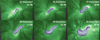 |
Fig. 6. Simulated flux rope where Tw > 1.0 is shown in a series of six panels from 11:36 UT on 25 December to 11:36 UT on 30 December, with a spacing of 24 h between each image. The flux ropes are plotted on top of the closest available AIA 94 Å observations (within 1 min) for each time step. |
3.4. The decay index
Next, we explored the physical mechanism by which the flux rope becomes unstable. In the case of torus instability (Bateman 1978; Kliem & Török 2006), a toroidal flux rope erupts if the overlying field decays sufficiently rapidly such that the confining Lorentz force can no longer counteract the radial hoop force of the flux rope. The decaying of the overlying field is quantified by the decay index, n:
 (7)
(7)
where Bex represents the overlying field due to external sources and h is the height. In idealised models, flux ropes are found to be torus-unstable when located in a region where n > 1.5. However, different values have been found in various studies, with Zuccarello et al. (2015) recently suggesting a range of 1.3−1.5, rather than a unique value. Moreover, in practical computations, it is not evident how to separate out the external field from the simulation given the complexity of the current systems. Consequently, we approximate the external field with the horizontal components of the potential field computed using the vertical component at the lower boundary as input data (Fan & Gibson 2007; Aulanier et al. 2010).
Plots of the contours from the decay index are shown in Fig. 7, including a vertical plane of the magnetic field-normalised current density (the magnitude of J divided by the magnitude of B) and contours of Tw. The first panel shows, at 11:36 UT on 26 December, a well-defined region of Tw > 1.0 within a region of increased current density, marking the location of the flux rope. Using the Tw contour in particular as an approximate boundary for the flux rope, we show that it formed close to the photosphere in a region where n < 1.0. In the second panel, at 11:36 UT on 27 December, the flux rope has risen and expanded and is approximately bisected by the n > 1.0 contour. In the third panel, at 11:36 UT on 28 December, the flux rope has risen and expanded further. At this time, the flux rope is located within a region where 2.0 > n > 1.0 and it has developed a region where Tw > 1.5, as described in Sect. 3.3 and marked by the cyan contour. In the final panel, at 11:36 UT on 29 December, the Tw > 1.0 region making up the flux rope is almost entirely within the region where n > 1.5.
 |
Fig. 7. Simulation excerpts from 11:36 UT on 26 December to 11:36 UT on 29 December, with a spacing of 24 h between each image. The plane depicts the current density (purple to green), with approximately horizontal contours of decay index (red to green) and additional contours of Tw (blue and cyan). The plane is in the same position as the Tw plane in Fig. 5. |
3.5. Relaxation simulations
To identify when our flux rope becomes unstable, we performed a series of relaxation simulations. A relaxation simulation is the same as the coronal magnetofrictional simulation described in Sect. 2, except that the photospheric driving is disabled (i.e. the driving horizontal electric field Eh = 0) at a specified time while the simulation continues. If the flux rope is inherently unstable in the simulation, it is expected to erupt without additional driving. We chose three different times to disable photospheric driving: at 12:00 UT on 27, 28, and 29 December, herein referred to as R1, R2, and R3, respectively. The results are depicted in Fig. 8, which shows the height of the flux rope axis over time for each of the three relaxation runs and the original simulation. The flux rope axis was computed by fitting a circle to contours of Tw and calculating the geometric centre.
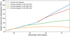 |
Fig. 8. Temporal evolution of flux rope height above the photosphere. Displayed: relaxation simulations where the driving was stopped at 12:00 on 27 December (orange, R1), at 12:00 on 28 December (green, R2), at 12:00 on 29 December (red, R3), and the original simulation where driving was not stopped (blue). |
In the case of R1, the flux rope does rise slightly but then settles into an equilibrium, which is accompanied by a decrease in Tw. In the R2 run, the flux rope does rise steadily, but at a slower rate than in the original simulation. This results in the flux rope being approximately halfway to the upper boundary by the time the simulation ends, and it appears that it would eject from the domain if allowed to continue. The curve for R3 is very similar to the original simulation, depicting a relatively quick rise but lagging slightly behind.
This behaviour is particularly notable when considered in parallel with the decay index shown in Fig. 7, whose panels were computed 24 min prior to the driving being disabled in each case. The R3 flux rope is shown to be almost entirely in a region where n > 1.5. Given that the flux rope went on to eject from the domain, this suggests that the flux rope was torus-unstable. Furthermore, given that the photospheric driving was disabled, it suggests that the flux rope went on to eject from the domain because of that instability. Figure 8 further suggests that the simulation would only produce an eruption following 12:00 UT on 27 December given that R1 settled into an equilibrium and that the flux rope would inevitably have erupted after 12:00 UT on 28 December; however further study would be required to determine the time of the eruption more accurately. We note that it is not a straightforward exercise to pinpoint the exact time of the eruption in MFM simulations (see discussion, e.g. in Pomoell et al. 2019). However, the flux rope was shown to be torus-unstable at a time that is consistent with the approximate observed eruption time of 12:00 UT on 28 December and its temporal evolution is well-matched by EUV observations (Fig. 6).
4. Conclusions
In this paper, we explore the evolution of the coronal magnetic field in AR 12473 using a time-dependent and data-driven magnetofrictional simulation. The boundary conditions for the simulation were obtained from the photospheric vector magnetic field observations and the non-inductive component was constructed using an optimisation approach based on an a priori assumption for the form of the non-inductive component. The value of the free parameter, U, was determined by optimising the total photospheric energy injection against DAVE4VM. Our simulation showed the formation of a well-defined flux rope that was ejected from the simulation domain and further analysis allowed us to explore its eruption mechanism.
The key findings of this study are:
-
The modelled magnetic field is visually consistent with EUV observations.
-
The core of the flux rope gets increasingly twisted as it rises, reaching Tw > 2.0 at the upper boundary of the simulation domain.
-
The rising flux rope pushes overlying fields out of the upper boundary as it rises and pushes neighbouring slightly twisted arcade-like loops to the side to erupt from between them.
-
The flux rope erupted as a result of the torus instability. In the relaxation simulation where the flux rope was initially within a region of decay index n > 1.5 it went on to rise and leave the domain, just as in the regular time-dependent, data-driven MFM simulation.
This study, therefore, demonstrates that the time-dependent, data-driven magnetofrictional method is a viable way of capturing the formation and initial evolution of eruptive solar flux ropes and that it can provide valuable insight into their eruption mechanism. Assessing the ability of the model to predict the magnetic structure of flux ropes in the heliosphere will form the basis of a future study.
Movies
Movie of Fig. 1 (94A) Access Supplementary Material
Movie of Fig. 1 (193A) Access Supplementary Material
Movie of Fig. 5 (Bz) Access Supplementary Material
Movie of Fig. 5 (Tw) Access Supplementary Material
Acknowledgments
This project has received funding from the European Research Council (ERC) under the European Union’s Horizon 2020 research and innovation programme (Grant agreement No. 724391). The work leading to these results has been carried out in the Finnish Centre of Excellence in Research of Sustainable Space (Academy of Finland grant number 312390). SDO data are courtesy of NASA/SDO and the AIA and HMI science teams. This research has made use of NASA’s Astrophysics Data System. EK and DP acknowledge the Finnish Society of Sciences and Letters and the Ruth och Nils-Erik Stenbäcks stipendium.
References
- Aulanier, G., Török, T., Démoulin, P., & DeLuca, E. E. 2010, ApJ, 708, 314 [Google Scholar]
- Bateman, G. 1978, MHD Instabilities (Cambridge, Mass.: MIT Press) [Google Scholar]
- Berger, M. A. 2003, in Topological Quantities in Magnetohydrodynamics, eds. A. Ferriz-Mas, & M. Núñez (CRC Press), 345 [Google Scholar]
- Brueckner, G. E., Howard, R. A., Koomen, M. J., et al. 1995, Sol. Phys., 162, 357 [NASA ADS] [CrossRef] [Google Scholar]
- Cheung, M. C. M., & DeRosa, M. L. 2012, ApJ, 757, 147 [NASA ADS] [CrossRef] [Google Scholar]
- Cheung, M. C. M., De Pontieu, B., Tarbell, T. D., et al. 2015, ApJ, 801, 83 [NASA ADS] [CrossRef] [Google Scholar]
- Domingo, V., Fleck, B., & Poland, A. I. 1995, Sol. Phys., 162, 1 [NASA ADS] [CrossRef] [Google Scholar]
- Eastwood, J. P., Hapgood, M. A., Biffis, E., et al. 2018, Space Weather, 16, 2052 [NASA ADS] [CrossRef] [Google Scholar]
- Fan, Y., & Gibson, S. E. 2007, ApJ, 668, 1232 [Google Scholar]
- Fisher, G. H., Welsch, B. T., Abbett, W. P., & Bercik, D. J. 2010, ApJ, 715, 242 [NASA ADS] [CrossRef] [Google Scholar]
- Fisher, G. H., Abbett, W. P., Bercik, D. J., et al. 2015, Space Weather, 13, 369 [NASA ADS] [CrossRef] [Google Scholar]
- Green, L. M., Kliem, B., & Wallace, A. J. 2011, A&A, 526, A2 [NASA ADS] [CrossRef] [EDP Sciences] [Google Scholar]
- Green, L. M., Török, T., Vršnak, B., Manchester, W., & Veronig, A. 2018, Space Sci. Rev., 214, 46 [Google Scholar]
- Kazachenko, M. D., Fisher, G. H., & Welsch, B. T. 2014, ApJ, 795, 17 [Google Scholar]
- Kilpua, E. K. J., Balogh, A., von Steiger, R., & Liu, Y. D. 2017, Space Sci. Rev., 212, 1271 [NASA ADS] [CrossRef] [Google Scholar]
- Kilpua, E. K. J., Lugaz, N., Mays, M. L., & Temmer, M. 2019, Space Weather, 17, 498 [NASA ADS] [CrossRef] [Google Scholar]
- Kliem, B., & Török, T. 2006, Phys. Rev. Lett., 96, 255002 [Google Scholar]
- Lemen, J. R., Title, A. M., Akin, D. J., et al. 2012, Sol. Phys., 275, 17 [Google Scholar]
- Lepping, R. P., Acũna, M. H., Burlaga, L. F., et al. 1995, Space Sci. Rev., 71, 207 [NASA ADS] [CrossRef] [Google Scholar]
- Liu, R., Kliem, B., Titov, V. S., et al. 2016, ApJ, 818, 148 [Google Scholar]
- Lumme, E., Pomoell, J., & Kilpua, E. K. J. 2017, Sol. Phys., 292, 191 [NASA ADS] [CrossRef] [Google Scholar]
- Pesnell, W. D., Thompson, B. J., & Chamberlin, P. C. 2012, Sol. Phys., 275, 3 [Google Scholar]
- Pomoell, J., Lumme, E., & Kilpua, E. 2019, Sol. Phys., 294, 41 [NASA ADS] [CrossRef] [Google Scholar]
- Price, D. J., Pomoell, J., Lumme, E., & Kilpua, E. K. J. 2019, A&A, 628, A114 [CrossRef] [EDP Sciences] [Google Scholar]
- Scherrer, P. H., Schou, J., Bush, R. I., et al. 2012, Sol. Phys., 275, 207 [Google Scholar]
- Schuck, P. W. 2008, ApJ, 683, 1134 [NASA ADS] [CrossRef] [Google Scholar]
- Schwenn, R. 2006, Liv. Rev. Sol. Phys., 3, 2 [Google Scholar]
- Slemzin, V. A., Goryaev, F. F., Rodkin, D. G., Shugay, Y. S., & Kuzin, S. V. 2019, Plasma Phys. Rep., 45, 889 [CrossRef] [Google Scholar]
- Sun, X., & Norton, A. A. 2017, Res. Notes Am. Astron. Soc., 1, 24 [NASA ADS] [CrossRef] [Google Scholar]
- van Ballegooijen, A. A., Priest, E. R., & Mackay, D. H. 2000, ApJ, 539, 983 [NASA ADS] [CrossRef] [Google Scholar]
- Vourlidas, A., Balmaceda, L. A., Stenborg, G., & Dal Lago, A. 2017, ApJ, 838, 141 [NASA ADS] [CrossRef] [Google Scholar]
- Welsch, B. T. 2018, Sol. Phys., 293, 113 [NASA ADS] [CrossRef] [Google Scholar]
- Wiegelmann, T., & Sakurai, T. 2012, Liv. Rev. Sol. Phys., 9, 5 [Google Scholar]
- Yang, W. H., Sturrock, P. A., & Antiochos, S. K. 1986, ApJ, 309, 383 [NASA ADS] [CrossRef] [Google Scholar]
- Yardley, S. L., Mackay, D. H., & Green, L. M. 2018, ApJ, 852, 82 [NASA ADS] [CrossRef] [Google Scholar]
- Zuccarello, F. P., Aulanier, G., & Gilchrist, S. A. 2015, ApJ, 814, 126 [NASA ADS] [CrossRef] [Google Scholar]
All Figures
|
Fig. 1. Series of AIA 193 Å observations depicting structures prior to the flare (left), shortly after the flare (middle), and four hours following the flare (right) that took place at approximately 11:20 UT. This figure is available as an online movie in the 94 Å and 193 Å channels. |
| In the text | |
|
Fig. 2. Temporal evolution of the photospheric energy injection for AR 12473. Displayed: optimised U (blue) and reference DAVE4VM (orange) totals. The vertical dotted line indicates the time of the M1.9 flare. |
| In the text | |
|
Fig. 3. Temporal evolution of the photospheric relative helicity injection for AR 12473. Displayed: optimised U (blue) and reference DAVE4VM (orange) totals. The vertical dotted line indicates the time of the M1.9 flare. |
| In the text | |
|
Fig. 4. Temporal evolution of volume metrics showing (a) the free magnetic energy (blue), magnetic energy (purple), and the ratio of the free to the total magnetic energy (orange); and (b) the current-carrying helicity (blue), relative helicity (purple), and the ratio of the current-carrying to the relative helicity (orange) for AR 12473. The vertical dotted line indicates the time of the M1.9 flare. |
| In the text | |
|
Fig. 5. Simulation excerpts from 11:36 UT on 28 December to 11:36 UT on 31 December with a spacing of 24 h between each image. Top row: flux rope for field lines where Tw > 1.5. It is bisected by a plane of Tw that also plots the contours of Tw. Bottom row: unobstructed view of the flux rope from the same angle. All plots include a plane of Bz at the lower boundary of the domain. The Tw and Bz planes are available as online movies. |
| In the text | |
|
Fig. 6. Simulated flux rope where Tw > 1.0 is shown in a series of six panels from 11:36 UT on 25 December to 11:36 UT on 30 December, with a spacing of 24 h between each image. The flux ropes are plotted on top of the closest available AIA 94 Å observations (within 1 min) for each time step. |
| In the text | |
|
Fig. 7. Simulation excerpts from 11:36 UT on 26 December to 11:36 UT on 29 December, with a spacing of 24 h between each image. The plane depicts the current density (purple to green), with approximately horizontal contours of decay index (red to green) and additional contours of Tw (blue and cyan). The plane is in the same position as the Tw plane in Fig. 5. |
| In the text | |
|
Fig. 8. Temporal evolution of flux rope height above the photosphere. Displayed: relaxation simulations where the driving was stopped at 12:00 on 27 December (orange, R1), at 12:00 on 28 December (green, R2), at 12:00 on 29 December (red, R3), and the original simulation where driving was not stopped (blue). |
| In the text | |
Current usage metrics show cumulative count of Article Views (full-text article views including HTML views, PDF and ePub downloads, according to the available data) and Abstracts Views on Vision4Press platform.
Data correspond to usage on the plateform after 2015. The current usage metrics is available 48-96 hours after online publication and is updated daily on week days.
Initial download of the metrics may take a while.