| Issue |
A&A
Volume 686, June 2024
|
|
|---|---|---|
| Article Number | A197 | |
| Number of page(s) | 6 | |
| Section | The Sun and the Heliosphere | |
| DOI | https://doi.org/10.1051/0004-6361/202348409 | |
| Published online | 12 June 2024 | |
The winding number of coronal flux ropes
I. Data-driven time-dependent magnetofrictional modelling
Department of Physics, University of Helsinki, Helsinki, Finland
e-mail: This email address is being protected from spambots. You need JavaScript enabled to view it.
Received:
27
October
2023
Accepted:
23
March
2024
Abstract
Context. Magnetic flux ropes are key structures in solar and solar-terrestrial research. Their magnetic twist is an important quantity for understanding their eruptivity, their evolution in interplanetary space, and their consequences for planetary space environments. The magnetic twist is expressed in terms of a winding number that describes how many times a field line winds about the axis of the flux rope (FR). Due to the complexity of calculating the winding number, current methods rely largely on its approximation.
Aims. We use a data-driven simulated FR to investigate the winding number Tg in comparison to the commonly used twist proxy Tw, which describes a winding of two infinitesimally close field lines. We also estimate the magnetic flux enclosed in the resultant FR(s).
Methods. We use the magnetic field analysis tools (MAFIAT) software to compute Tg and Tw for data-driven time-dependent magnetofrictional modelling of AR12473.
Results. We find that the FR boundaries can significantly differ depending on whether they are defined using the twist approximation Tw or the winding number Tg. This also significantly affects the FR structure and the estimates of the enclosed magnetic flux. For the event analysed here, Tg also reveals that the twisted flux system consists of two separate intertwined FRs.
Conclusions. The results of this study suggest that the computation of the winding number (Tg) is important for investigations of solar FRs.
Key words: magnetic fields / methods: data analysis / methods: numerical / Sun: corona / Sun: coronal mass ejections (CMEs)
© The Authors 2024
 Open Access article, published by EDP Sciences, under the terms of the Creative Commons Attribution License (https://creativecommons.org/licenses/by/4.0), which permits unrestricted use, distribution, and reproduction in any medium, provided the original work is properly cited.
This article is published in open access under the Subscribe to Open model. This email address is being protected from spambots. You need JavaScript enabled to view it. to support open access publication.
1. Introduction
Coronal mass ejections are enormous eruptions of plasma and magnetic field from the Sun, and are one of the primary drivers of space weather in the heliosphere (CMEs; e.g. Slemzin et al. 2019; Webb & Howard 2012). At their core, CMEs have a flux rope (FR) comprised of helical magnetic fields winding about a common axis (e.g. Chen 2017). The properties of FRs influence the eruption and the subsequent evolution of the CME through the corona and interplanetary space, and eventually the consequences the CME might have on Earth or other planets in the Solar System (e.g. Kilpua et al. 2017). Thus, a thorough understanding of how and by which physical mechanisms FRs form, become unstable, and evolve is necessary to fully comprehend CMEs and to forecast their space weather consequences.
A fundamental property of all magnetic FRs is the magnetic helicity that measures the twisting and writhing of the magnetic field. Magnetic twist describes how many turns a field line completes about the axis of a FR while writhing represents the global kinking of the axis of the rope (e.g. Berger & Field 1984; Berger & Prior 2006). One of the key reasons why magnetic helicity is considered such a central parameter in solar physics is that it is conserved in the case of large magnetic Reynold’s numbers (e.g. in space plasmas), and is conserved with good approximation in magnetohydrodynamic processes with low resistivity, such as in magnetic reconnection (e.g. Berger & Field 1984). However, the type of magnetic helicity (i.e. twist or writhe) can change or can be transferred from one region to another; for example, it can be first injected into the photosphere (e.g., Demoulin et al. 2006) before moving into the corona where it is finally shed away from the Sun into interplanetary space by CMEs (e.g. DeVore 2000; Démoulin et al. 2002; Green et al. 2002).
Magnetic helicity and twist have also been established as important proxies with which to investigate and predict CME eruptivity. Magnetic twist accumulates in coronal structures, increasing helicity and free magnetic energy, and the eruption takes place when a critical threshold is exceeded (e.g. Liokati et al. 2022). The resulting process, where twist is transferred into writhe, is called a kink instability (Török et al. 2004), and the FR may then explosively reconnect. However, a broad range of critical twist values are reported in the literature, depending on the methods employed to investigate the AR in question and the assumptions of the FR.
At present, the magnetic field cannot be observed with good accuracy in the tenuous and hot corona, and therefore detailed studies of erupting solar FRs rely on extrapolations and simulations. The key issue is therefore the identification of FRs and calculating twist from the simulation outputs. The theoretical work defining twist metrics was outlined by Berger & Prior (2006). The rigorous definition of the twist in flux ropes, as stated previously, includes a calculation of the winding of the field lines about the axis of the FR. This can be done by integrating the rotation rate of a target field line about a defined axis. The calculation of the twist in this manner is an involved non-trivial process (Price et al. 2022). Therefore, most previous studies (e.g. Garland et al. 2023; Yamasaki et al. 2022; Price et al. 2019, 2022; Duan et al. 2022) approximated the winding number by calculating how many times two infinitesimally close field lines wind about each other. This definition for the twist was also given in Berger & Prior (2006). Liu et al. (2016) denoted the twist number that measures the winding about the defined axis (i.e. the winding number) as Tg and the twist number calculated from the winding of two infinitesimally close adjacent field lines as Tw. We adopt the same terminology here. Liu et al. (2016) also compared these two twist metrics and concluded that they generally match close to the axis of the FR, but can deviate significantly elsewhere.
However, the winding number Tg was recently applied in multiple studies to investigate eruptive solar magnetic fields (e.g. Duan et al. 2023; Yu et al. 2023) and open source tools exist to facilitate its calculation (e.g. Price et al. 2022). For example, Duan et al. (2023) investigated a large X-class flare and the related FR eruption from AR 12887 (central meridian passage on 28 October 2021). The analysis of twist using a non-linear force-free field (NLFFF) extrapolation showed that the critical threshold for the kink instability was not exceeded and no signature of writhing of the axis was detected in observations. The authors suggested that the eruption was initiated by reconnection and that the FR was driven away from the Sun due to the torus instability. The temporal evolution of twist metrics Tg and Tw was also compared and some systematic differences were found.
Despite Tg being a reliable proxy for twist for all field lines in the FR, its use is still very limited. In the present study, we performed a twist-based analysis of the time-dependent data-driven magnetofrictional simulation of NOAA Active Region (AR) 12473 conducted by Price et al. (2020). We first investigated the choice of the FR axis that is crucial for the computation of Tg. In particular, we demonstrate how the use of Tw as a twist metric can result in one FR, while Tg results in two distinct FRs and offers the possibility to determine which field lines belong to each FR. We then explored how the domain where Tg is calculated can be constrained by Tw. In principle, Tg can be calculated for the whole simulation plane, but as this is computationally inefficient and relatively resource intensive, it is much more feasible to constrict the area. We define how different Tw criteria defining this domain affect the FR boundaries and the enclosed magnetic flux values.
The paper is organised as follows. In Sect. 2, we summarise the data used and the analytical methods employed. In Sect. 3, we present and interpret the results. Finally, in Sect. 4, we present our key findings and conclusions.
2. Data and methods
This study concerns the output from the time-dependent data-driven magnetofrictional simulation of AR 12473 presented in detail in Price et al. (2020). Readers are directed to Pomoell et al. (2019) and Price et al. (2020) for the details of the model and the reasoning behind its use. It is important to emphasise that the methods applied in this study are independent of the model used. The authors employed the commonly used twist number Tw (Liu et al. 2016) to identify the FR in their simulation and explore the magnetic field topology. The output of the simulation is of interest to this work because of the difficulty in interpreting the structure of Tw (see online movies in Price et al. 2020) during the formation of the FR and its rise through the domain. A visually complex twist structure can, for example, make it difficult to resolve the detailed flux rope topology, and therefore to discern whether it consists of a single coherent flux rope or potentially of multiple intertwined components.
We focus on the simulation output at 11:36 UT on 30 December, 2015 because the FR at this point was fully formed and rising steadily through the simulation domain but had not yet reached the top of the domain where boundary effects may come into play. The Tw map at x = 0 is plotted in Fig. 1 and highlights a visually complex Tw structure. The Tw = 1.0 contour has a distinctly irregular shape but the contour is unbroken, rather than being multiple independent contours. This is in contrast to the multiple and spatially distinct Tw = 1.2 contours for example.
Here, we use the Tw = 1.0 contour to approximately outline the FR because a FR is commonly defined as a coherent structure of field lines winding about a common axis with a winding number of at least one, which means that the field line has to do at least one full turn about the axis of the FR. This definition has been used to locate and extract flux ropes from simulation domains in several studies (e.g. Wagner et al. 2023; Kumari et al. 2023; Lumme et al. 2022; Yamasaki et al. 2022; Kilpua et al. 2021; Price et al. 2020).
We use the method described in Liu et al. (2016) to define the axis of the FR. The authors show that the axis of an FR may be found as an extremum of Tw. As demonstrated in more detail in the following section, in the studied December 2015 eruption, applying the principle of the axis being located at an extremum of Tw (Price et al. 2022) is non-trivial due to the complexity of the Tw map.
As described in Sect. 1, the winding number describes the degree to which FR field lines wind about a common axis. However, an approximation of the winding number is often used due to the relative simplicity of its computation, in contrast to the rigorous definition. The most common method relies on computing how many times two infinitesimally close field lines wind about each other. The formulation of this Tw metric is as follows (Liu et al. 2016; Berger & Prior 2006):
 (1)
(1)
where L denotes the curve defined by the field line. This metric only reliably approximates the winding number close to the FR axis, where the infinitesimally close description holds. However, as the distance from the axis increases, Tw tends to under- or overestimate the winding number of each field line.
The twist number Tg that describes the winding of the field lines about a defined axis is given as (Liu et al. 2016; Berger & Prior 2006):
 (2)
(2)
where x(s) defines the flux rope axis, φ the rotation angle made by the field line under consideration about x(s),  the unit tangent vector to x(s), and
  the unit vector normal to x(s), which intersects the field line in question.
As noted in Sect. 1, in this study we use the open-source MAFIAT (magnetic field analysis tools) Python software (Price et al. 2022) to compute both the winding number Tg and the approximation, Tw.
3. Results and discussion
3.1. Identifying the FR axis
For the computation of Tg, the definition of the FR axis is paramount. For the event analysed in this paper, the Tw maps given in Fig. 1 show several potential Tw maxima that are connected by one coherent, but complex Tw = 1.0 contour. We note that partly different contour thresholds are used in the left and right panels of Fig. 1 to highlight the two maxima studied in this work. Price et al. (2020) attributed the FR to the large, almost self-contained Tw ≥ 1.0 region in the upper part of Fig. 1, while the authors truncated the L-shaped Tw ≥ 1.0 region beneath and to the left of the upper structure. These two regions are separated by a dashed green curve in the first panel. However, the two well-defined maxima of Tw indicated by lime green dots in the left and right panels of Fig. 1 may represent axes of two separate FRs.
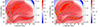 |
Fig. 1. Vertical cross-sections, which correspond to the blue boxes in Fig. 2, of the Tw twist metric map at x = 0 Mm, showing a complex but connected structure that likely consists of two separate FRs. The lime green dots indicate the location of the axes for the upper (left) and lower (right) FRs. The Tw contours have slightly different thresholds in the left and right panels to highlight the two Tw maxima. The dashed green curve separates the almost self-contained Tw ≥ 1.0 region used by Price et al. (2020) on the right from the rest of the structure as described in Sect. 3.1. |
In this paper, in contrast to Price et al. (2020), we consider the entire Tw ≥ 1.0 region and compute the associated Tg profile for each of the two candidate axes with the MAFIAT code. We name here the structures based on their relative position in the twist map as the “upper FR”, whose axis is shown as a green dot in the left part of Fig. 1, and the “lower FR”, whose axis is shown as a green dot in the right panel of the same figure.
The first two panels of Fig. 2 illustrate the overall structure of the upper and lower FRs by showing the magnetic field lines that satisfy Tg ≥ 1.0 plotted for their respective axes. The third panel shows a combination of the upper two panels and the fourth panel shows their axes. The final panel (e) shows field lines that satisfy Tw ≥ 1.0. The corresponding Tg and Tw distributions are shown in Fig. 3. We remind the reader that the Tg ≥ 1.0 requirement corresponds to the common definition of an FR, which states that a field line has to make at least one full turn about the axis, while Tw only strictly matches that definition at the axis.
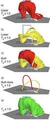 |
Fig. 2. Field lines corresponding to the contour boundaries of Fig. 3. The field of view of Fig. 3 and the aforementioned contours are overplotted in blue. Additionally, we show lines corresponding to the Tg = 1.0 contour for the upper axis (a), the Tg = 1.0 contour for the lower axis (b), for the previous two cases combined (c), for the axes of the previous two cases combined (d), and for the Tw = 1.0 contour (e). All panels include a plane of Bz from the lower boundary of the simulation domain. |
Figure 3 shows that generally, the two axes result in two independent structures. When the axis of the “upper FR” is selected, the majority of the field lines from the “lower FR” region return NaN (black) values for Tg (panel (a) of Fig. 3). This happens in MAFIAT when the code is unable to locate normal vectors for almost all points along the axis to the target field line in a “fitting” process (Price et al. 2022). Similarly, when the axis of the “lower FR” is selected, the majority of the field lines from the “upper FR” region are not fitted and return NaN values (panel (b) of Fig. 3). In other words, these two axes separate the one coherent Tw structure into two separate FRs. However, we note that there is a small region of overlap between the Tg = 1.0 contours for the two axes, which is highlighted by the green dashed-circles in Fig. 3.
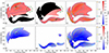 |
Fig. 3. Output for the Tw ≥ 1.0 mask. The first row shows Tg for the upper and lower FRs (a, b), and Tw (c) with isocontours and colour maps of their respective twist metrics. The second row shows the signed flux for the upper and lower FRs (d, e), and for the Tw region (f) with the same isocontours as the first row and colour maps of signed flux. The green dashed-circles highlight overlapping regions and the black arrow indicates a particular feature, both described in Sect. 3.1. |
The upper axis (first column, Fig. 3) reveals the FR structure that largely corresponds to that analysed in Price et al. (2020), with the addition of the left-most region (black arrow). This FR structure appears to be the most significant coherent bundle of field lines in the displayed cross-section. The Tg = 1.0 contour (dark blue) has a deformed oval shape.
The lower axis (second column, Fig. 3) results in a considerably more complex structure beneath the upper FR; its shape is not consistent with the common view that FRs have nearly circular or elliptical cross-sections. Instead, the Tg = 1.0 boundary now has a shape reminiscent of a figure of eight. The comparison of the simulation snapshots containing the upper and lower FRs combined (Fig. 2c) to the FR defined using the Tw ≥ 1.0 criteria (Fig. 2e) reveals why for this AR, when using the Tw ≥ 1.0 criteria for the FR identification, it is easy to mistake the structure for a single FR. The two FRs combined indeed visually resemble one coherent FR.
However, when the two structures from the Tg analysis are plotted separately (Figs. 2a and b), differences in their magnetic connectivity to the photosphere become apparent. While on the left the field lines connect to the same negative-polarity footpoint (black region), the positive-polarity footpoints on the right primarily connect to different regions (white regions). The field lines belonging to the lower FR primarily connect to a separate positive-polarity region slightly west (right) of the positive polarity region where the field lines from the upper FR connect. This is highlighted by Fig. 2d, which shows where the axes of the two structures connect to the photosphere.
The snapshots showing field lines in Fig. 2 also add clarity to the previously discussed small region of overlapping Tg = 1.0 contours (Figs. 3a and b) between the field lines resulting from the upper and lower axis. The small collection of separate field lines arching over the lower FR in Fig. 2b correspond to the region in the top of Fig. 3b (green dashed-circle). However, their shape and footpoint connectivity suggest that they belong to the upper FR.
3.2. Identifying FR boundaries
Here we investigate how the commonly applied constraint of |Tw|≥1.0 can affect the resulting FR. Here, we calculate Tg in an area that is defined by different Tw criteria (“masks”). By comparing how the Tg = 1.0 boundary contour changes for different masks of Tw we can identify, for example, how much of the FR structure may have been missed by the application of a simple Tw ≥ 1.0 constraint on the simulation output. For our positively twisted FR, we apply tests of Tw ≥ 1.0, 0.9, and 0.8 and explore the corresponding Tg output. The results for Tw ≥ 1.0 and Tw ≥ 0.8 are shown in Figs. 3 and 4, respectively.
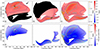 |
Fig. 4. Output for the Tw ≥ 0.8 mask. The first row shows Tg for the upper and lower FRs (a, b), and Tw (c) with isocontours and colour maps of their respective twist metrics. The second row shows the signed flux for the upper and lower FRs (d, e), and for the Tw region (f) with the same isocontours as the first row and colour maps of signed flux. The black arrow indicates a feature described in Sect. 3.1. |
For example, Figs. 3a and b show Tg calculated for the “upper FR” and the “lower FR”, respectively, in a domain corresponding to the Tw ≥ 1.0 mask shown in Fig. 3c. The comparison of panels (a) and (c) reveals that the Tg = 1.0 contour deviates considerably from the Tw = 1.0 contour in the upper part of the plot. The Tg = 1.0 contour encompasses a considerably smaller area as it does not extend to the low Y values reached by the Tw = 1.0 contour. This will naturally have an effect on any quantities sensitive to FR area, such as flux.
As the mask is decreased to Tw ≥ 0.80, a gap starts to appear between the Tg = 1.0 contour and the edge of the right-hand side region (black arrow, Fig. 4a). This suggests that the Tw ≥ 1.0 masking leads to underestimation of the twist in that region. Despite lowering the mask, the leftmost extent of the Tg = 1.0 contours remains unchanged. This is due to the region already being at its fullest extent with respect to the leftmost boundary. As shown by the Tw = 1.0 contour in Fig. 1, its leftmost parts are against the boundary where the twist changes from positive (red) to negative (blue).
The analysis above shows that the upper axis results in an FR that remains relatively unchanged when the region where Tg is calculated is increased (i.e. the Tw mask criterion decreases). In contrast, using the lower axis results in structures that show significant variations (second column of Figs. 3 and 4). For the Tw ≥ 1.0 mask, two contours of Tg = 1.0 appear at the upper part of the plot that are not connected directly to the axis (Fig. 3b). This suggests that the field lines of the lower FR are not fully captured by the Tw ≥ 1.0 mask. When the Tw ≥ 0.8 mask is applied, these detached regions ultimately all connect (Fig. 4b); that is, when Tg is calculated in a sufficiently large region. Comparing the final shape to Fig. 1 suggests that decreasing the mask uncovers more of the lower structure. However, the spiky shape of the right boundary in Fig. 4 may mean that there are simply relatively positively twisted neighbouring field lines that are not part of the structure.
3.3. Effects on flux
For both axes and each Tw mask, we also computed the corresponding magnetic flux through the domain enclosed by the Tg ≥ 1.0 curves. For the Tw ≥ 1.0 and Tw ≥ 0.8 cases, these are shown in the two first panels in the bottom row of Figs. 3 and 4. The last panel in the bottom row in these figures gives the flux through the Tw masked planes. The corresponding total magnetic flux values are summarised in Table 1.
Magnetic fluxes in the units of 1021 Maxwells through the structures extracted using different twist metrics and masks.
As expected, the fluxes increase as the Tw mask decreases in all investigated cases. This is expected as the field lines fulfilling the mask criteria increase as the Tw threshold is relaxed. In other words, when the mask is lower, more field lines are included. Compared to the Tw ≥ 1.0 region, the Tw ≥ 0.8 region shows a 28.3% increase in flux. Correspondingly, the flux through the upper FR increases by 10.3% and that through the lower FR by 49.4%. This is consistent with the changing FR boundaries described in Sect. 3.2; though the increase for the lower FR is particularly significant (see Table 2).
In each case, the upper FR clearly accounts for a larger fraction of the total flux through the Tw ≥ 1.0 plane than the lower FR. For the Tw ≥ 1.0 mask, this fraction is 46.9% of the total, decreasing to 40.3% for the Tw ≥ 0.8 mask. For the lower FR, the corresponding percentages are 16.7% and 19.5%. This leaves approximately 40% of the total flux through the Tw region that does not belong to the flux rope structures defined with the Tg twist metric for each mask. This illustrates the significant effect on flux calculations when identifying flux ropes by simple Tw boundaries compared to a thorough Tg analysis.
3.4. Flux-weighted twist averages
We also computed the flux-weighted averages of Tw and Tg as in Eqs. (2) and (4) of Duan et al. (2023). However, while their values were constrained based on the FR definition of Tw ≥ 1.0, we additionally computed the flux-weighted averages using the definition of Tg ≥ 1.0 following the significant differences noted in the preceding sections. We define these as
 (3)
(3)
 (4)
(4)
where S denotes a cross section of the FR and Bn the magnetic field component normal to the slice. The resulting averages are shown by Table 3. While our analysis is for a single time step, the values from the Tw ≥ 1.0 condition are similar to those found by Duan et al. (2023) in the sense that (Tw)mean far exceeds (Tg)mean, albeit to a lesser degree. It is notable that the values from the Tg ≥ 1.0 condition are very similar, both to each other, and also to the (Tw)mean of the Tw ≥ 1.0 condition. This similarity further illustrates the need for visual analysis of the flux ropes and their twist distributions to ensure accuracy.
Flux-weighted averages of both twist metrics, constrained by each FR boundary definition.
4. Conclusions
In this study, we explored the magnetic structures in the time-dependent data-driven magnetofrictional model of AR 12473 of Price et al. (2020). To this end, we used the twist metrics Tw (Eq. (1)), which is based on parallel current and the magnetic field, and Tg (Eq. (2)), which is based on the field line geometry. Tg can be considered to express the definitive twist of a magnetic flux rope because it calculates the winding number; that is, the number of times a magnetic field line winds about the axis of the flux rope. Tw instead calculates the winding of two infinitesimally close field lines. We assessed the similarities and differences between these twist metrics visually (Fig. 2) and via toroidal flux computations (Sect. 3.3). The key findings of this study can be summarised as follows:
-
When applied to a real case, Tw may both under- and over-estimate the winding number in different parts of the flux rope.
-
There can be significant differences between FRs defined by Tw and Tg, resulting in significant differences in flux values.
-
The interpretation of flux-weighted average twists requires supporting visual analysis.
-
Computation of Tg is necessary for reliable identification of FR boundaries.
However, we note that the calculation of Tw is a critical part of our Tg determination. Firstly, the axis of the flux rope is located based on the extremum of Tw. Secondly, we demonstrate that Tw can be used to constrain the region where Tg is calculated.
While this single case study is not representative of all CME flux ropes, it does serve to illustrate the potential for error in cases where FR identification relies on Tw alone. There will likely be cases where the differences between the boundaries and fluxes for Tw and Tg will be smaller than in this case, but they could similarly be larger. The twist analysis tool MAFIAT (Price et al. 2022), which enables straightforward calculation and visualisation of the winding number Tg, provides a basis for the future extension of this work to a larger number of events.
Acknowledgments
This project has received funding from the European Research Council (ERC) under the European Union’s Horizon 2020 research and innovation programme under grant agreement No. 724391 (SolMAG) and 101004159 (SERPENTINE). The work leading to these results has been carried out in the Finnish Centre of Excellence in Research of Sustainable Space (Academy of Finland grant number 336807). J.P. acknowledges the Academy of Finland Project 343581 (SWATCH). SDO data are courtesy of NASA/SDO and the AIA and HMI science teams. This research has made use of NASA’s Astrophysics Data System.
References
- Berger, M. A., & Field, G. B. 1984, J. Fluid Mech., 147, 133 [NASA ADS] [CrossRef] [Google Scholar]
- Berger, M. A., & Prior, C. 2006, J. Phys. A Math. Gen., 39, 8321 [Google Scholar]
- Chen, J. 2017, Phys. Plasmas, 24, 090501 [Google Scholar]
- Démoulin, P., Mandrini, C. H., van Driel-Gesztelyi, L., et al. 2002, A&A, 382, 650 [NASA ADS] [CrossRef] [EDP Sciences] [Google Scholar]
- Demoulin, P., Pariat, E., & Berger, M. A. 2006, Sol. Phys., 233, 3 [CrossRef] [Google Scholar]
- DeVore, C. R. 2000, ApJ, 539, 944 [Google Scholar]
- Duan, A., Jiang, C., Guo, Y., Feng, X., & Cui, J. 2022, A&A, 659, A25 [NASA ADS] [CrossRef] [EDP Sciences] [Google Scholar]
- Duan, A., Jiang, C., Zhou, Z., & Feng, X. 2023, A&A, 674, A192 [NASA ADS] [CrossRef] [EDP Sciences] [Google Scholar]
- Garland, S. H., Yurchyshyn, V. B., Loper, R. D., Akers, B. F., & Emmons, D. J. 2023, Front. Astron. Space Sci., 10, 64 [NASA ADS] [CrossRef] [Google Scholar]
- Green, L. M., López fuentes, M. C., Mandrini, C. H., et al. 2002, Sol. Phys., 208, 43 [Google Scholar]
- Kilpua, E., Koskinen, H. E. J., & Pulkkinen, T. I. 2017, Liv. Rev. Sol. Phys., 14, 5 [Google Scholar]
- Kilpua, E. K. J., Pomoell, J., Price, D., Sarkar, R., & Asvestari, E. 2021, Front. Astron. Space Sci., 8, 35 [NASA ADS] [CrossRef] [Google Scholar]
- Kumari, A., Price, D. J., Daei, F., Pomoell, J., & Kilpua, E. K. J. 2023, A&A, 675, A80 [NASA ADS] [CrossRef] [EDP Sciences] [Google Scholar]
- Liokati, E., Nindos, A., & Liu, Y. 2022, A&A, 662, A6 [NASA ADS] [CrossRef] [EDP Sciences] [Google Scholar]
- Liu, R., Kliem, B., Titov, V. S., et al. 2016, ApJ, 818, 148 [Google Scholar]
- Lumme, E., Pomoell, J., Price, D. J., et al. 2022, A&A, 658, A200 [NASA ADS] [CrossRef] [EDP Sciences] [Google Scholar]
- Pomoell, J., Lumme, E., & Kilpua, E. 2019, Sol. Phys., 294, 41 [NASA ADS] [CrossRef] [Google Scholar]
- Price, D. J., Pomoell, J., Lumme, E., & Kilpua, E. K. J. 2019, A&A, 628, A114 [NASA ADS] [CrossRef] [EDP Sciences] [Google Scholar]
- Price, D. J., Pomoell, J., & Kilpua, E. K. J. 2020, A&A, 644, A28 [NASA ADS] [CrossRef] [EDP Sciences] [Google Scholar]
- Price, D. J., Pomoell, J., & Kilpua, E. K. J. 2022, Front. Astron. Space Sci., 9, 407 [NASA ADS] [CrossRef] [Google Scholar]
- Slemzin, V. A., Goryaev, F. F., Rodkin, D. G., Shugay, Y. S., & Kuzin, S. V. 2019, Plasma Phys. Rep., 45, 889 [NASA ADS] [CrossRef] [Google Scholar]
- Török, T., Kliem, B., & Titov, V. S. 2004, A&A, 413, L27 [NASA ADS] [CrossRef] [EDP Sciences] [Google Scholar]
- Wagner, A., Kilpua, E. K. J., Sarkar, R., et al. 2023, A&A, 677, A81 [NASA ADS] [CrossRef] [EDP Sciences] [Google Scholar]
- Webb, D. F., & Howard, T. A. 2012, Liv. Rev. Sol. Phys., 9, 3 [Google Scholar]
- Yamasaki, D., Inoue, S., Bamba, Y., Lee, J., & Wang, H. 2022, ApJ, 940, 119 [NASA ADS] [CrossRef] [Google Scholar]
- Yu, F., Zhao, J., Su, Y., et al. 2023, ApJ, 951, 54 [CrossRef] [Google Scholar]
All Tables
Magnetic fluxes in the units of 1021 Maxwells through the structures extracted using different twist metrics and masks.
Flux-weighted averages of both twist metrics, constrained by each FR boundary definition.
All Figures
|
Fig. 1. Vertical cross-sections, which correspond to the blue boxes in Fig. 2, of the Tw twist metric map at x = 0 Mm, showing a complex but connected structure that likely consists of two separate FRs. The lime green dots indicate the location of the axes for the upper (left) and lower (right) FRs. The Tw contours have slightly different thresholds in the left and right panels to highlight the two Tw maxima. The dashed green curve separates the almost self-contained Tw ≥ 1.0 region used by Price et al. (2020) on the right from the rest of the structure as described in Sect. 3.1. |
| In the text | |
|
Fig. 2. Field lines corresponding to the contour boundaries of Fig. 3. The field of view of Fig. 3 and the aforementioned contours are overplotted in blue. Additionally, we show lines corresponding to the Tg = 1.0 contour for the upper axis (a), the Tg = 1.0 contour for the lower axis (b), for the previous two cases combined (c), for the axes of the previous two cases combined (d), and for the Tw = 1.0 contour (e). All panels include a plane of Bz from the lower boundary of the simulation domain. |
| In the text | |
|
Fig. 3. Output for the Tw ≥ 1.0 mask. The first row shows Tg for the upper and lower FRs (a, b), and Tw (c) with isocontours and colour maps of their respective twist metrics. The second row shows the signed flux for the upper and lower FRs (d, e), and for the Tw region (f) with the same isocontours as the first row and colour maps of signed flux. The green dashed-circles highlight overlapping regions and the black arrow indicates a particular feature, both described in Sect. 3.1. |
| In the text | |
|
Fig. 4. Output for the Tw ≥ 0.8 mask. The first row shows Tg for the upper and lower FRs (a, b), and Tw (c) with isocontours and colour maps of their respective twist metrics. The second row shows the signed flux for the upper and lower FRs (d, e), and for the Tw region (f) with the same isocontours as the first row and colour maps of signed flux. The black arrow indicates a feature described in Sect. 3.1. |
| In the text | |
Current usage metrics show cumulative count of Article Views (full-text article views including HTML views, PDF and ePub downloads, according to the available data) and Abstracts Views on Vision4Press platform.
Data correspond to usage on the plateform after 2015. The current usage metrics is available 48-96 hours after online publication and is updated daily on week days.
Initial download of the metrics may take a while.