| Issue |
A&A
Volume 677, September 2023
|
|
|---|---|---|
| Article Number | A81 | |
| Number of page(s) | 12 | |
| Section | The Sun and the Heliosphere | |
| DOI | https://doi.org/10.1051/0004-6361/202346260 | |
| Published online | 08 September 2023 | |
The automatic identification and tracking of coronal flux ropes
I. Footpoints and fluxes⋆
1
Department of Physics, University of Helsinki, PO Box 64 00014 Helsinki, Finland
e-mail: This email address is being protected from spambots. You need JavaScript enabled to view it.
2
CmPA/Department of Mathematics, KU Leuven, Celestijnenlaan 200B, 3001 Leuven, Belgium
3
Institute of Physics, University of Maria Curie-Skłodowska, ul. Radziszewskiego 10, 20-031 Lublin, Poland
4
NASA Goddard Space Flight Center, Greenbelt, MD 20771, USA
Received:
27
February
2023
Accepted:
17
May
2023
Abstract
Context. Investigating the early-stage evolution of an erupting flux rope from the Sun is important for understanding the mechanisms of how it loses its stability and its space-weather impact.
Aims. Our aim is to develop an efficient scheme for tracking the early dynamics of erupting solar flux ropes and to use the algorithm to analyse its early-stage properties. The algorithm is tested on a data-driven simulation of an eruption that took place in active region AR12473. We investigate the modelled footpoint movement and magnetic flux evolution of the flux rope and compare these with observational data from the Solar Dynamics Observatory (SDO) Atmospheric Imaging Assembly (AIA) in the 211 Å and 1600 Å channels.
Methods. We used the time-dependent data-driven magnetofrictional model (TMFM) to carry out our analysis. We also performed another modelling run, where we stop the driving of the TMFM midway through the rise of the flux rope through the simulation domain and evolve it instead with a zero-beta magnetohydrodynamic (MHD) approach.
Results. The developed algorithm successfully extracts a flux rope and its ascent through the simulation domain. We find that the movement of the modelled flux rope footpoints showcases similar trends in both the TMFM and relaxation MHD runs: the footpoints recede from their respective central location as the eruption progresses and the positive polarity footpoint region exhibits a more dynamic behaviour. The ultraviolet (UV) brightenings and extreme ultraviolet (EUV) dimmings agree well with the models in terms of their dynamics. According to our modelling results, the toroidal magnetic flux in the flux rope first rises and then decreases. In our observational analysis, we capture the descending phase of toroidal flux.
Conclusions. The extraction algorithm enables us to effectively study the early dynamics of the flux rope and to derive some of its key properties, such as footpoint movement and toroidal magnetic flux. The results generally agree well with observational data.
Key words: Sun: corona / Sun: activity / methods: observational / Sun: magnetic fields / Sun: coronal mass ejections (CMEs) / methods: data analysis
Movies associated with Fig. 2 are available at https://www.aanda.org.
© The Authors 2023
 Open Access article, published by EDP Sciences, under the terms of the Creative Commons Attribution License (https://creativecommons.org/licenses/by/4.0), which permits unrestricted use, distribution, and reproduction in any medium, provided the original work is properly cited.
This article is published in open access under the Subscribe to Open model. This email address is being protected from spambots. You need JavaScript enabled to view it. to support open access publication.
1. Introduction
Coronal mass ejections (CMEs) are the largest of the solar eruptions and are key drivers of space weather on Earth and other planets of our Solar System. Their formation, properties, and evolution are therefore of major interest for the space physics community, both for accurately forecasting their space weather consequences and understanding their underlying physics.
The common consensus is that magnetic flux ropes (FRs) are an integral part of CMEs (e.g. Chen 2017; Green et al. 2018). A FR is a coherent magnetic structure where the magnetic field lines wind around a common axis. Direct observations of Earth-impacting CME FRs are usually available only at the Lagrangian point L1. Otherwise, we need to rely on occasional observational signatures at distances closer to the Sun or on remote-sensing observations. The kinematic and geometric properties of CME FRs can be inferred from white-light coronagraph observations, but there are currently no suitable observations with which to measure the magnetic field in CME FRs remotely in a consistent manner (e.g. Kilpua et al. 2019). One can use a combination of indirect observational proxies to infer the magnetic properties of CME FRs (Palmerio et al. 2017), but suitable observations or necessary signatures may not always be available. Another key issue is that the formation and early evolution of CMEs in the low corona are poorly understood. This is a severe limitation as CMEs may experience strong dynamics during this early state as they lift off from the Sun.
The evolution of CMEs can also be studied with numerical simulations. One of the advanced approaches is data-driven modelling, which uses a time series of observational data to model the time-evolution of the coronal magnetic field (Cheung & DeRosa 2012; Mackay et al. 2011). The modelling of the CME FR can be used to infer many of its key properties such as its magnetic twist, enclosed magnetic flux, and the location of the footpoints. The analysis of footpoints not only provides information about where the CME is rooted at the Sun, but can also reveal clues as to their movement, which can reveal important aspects of their early dynamics. However, interpretations of FR observations close to the Sun are often complicated and ambiguous and their comparison with modelling results is not straightforward. Footpoints of CME FRs may manifest themselves in remote-sensing ultraviolet (UV) and extreme ultraviolet (EUV) observations, both as localised dimmings and brightenings.
The coronal dimmings refer to a localised transient decrease in the emission intensity in the vicinity of the eruption site (e.g. Thompson et al. 1998). The CME FR footpoints are believed to manifest as strong (in terms of change in intensity) and localised ‘core’ or ‘twin dimmings’, which are found close to the eruption site (Webb et al. 2000; Dissauer et al. 2018). Often, ‘secondary dimmings’ are also observed, which appear shallower and usually spread much further (see e.g. Veronig et al. 2019; Mandrini et al. 2007; Dissauer et al. 2018).
The dominant cause of coronal dimmings is believed to be the evacuation of plasma in the wake of the CME and/or its expansion, but several other sources may contribute to the dimming, such as thermal, obscuration, and wave dimming (e.g. Cheng & Qiu 2016). Therefore, core dimmings are generally thought of as indicating the anchoring footpoints of the CME FR (Webb et al. 2000; Dissauer et al. 2018) and the evolution of the dimming can provide unique information on the early evolution of the CME. In addition, core dimmings have been used to estimate the magnetic flux enclosed in the CME (Mandrini et al. 2005; Webb et al. 2000; Attrill et al. 2006). However, many effects can interfere with the appearance of core dimmings that are not related to the FR footpoints, and sometimes even no dimmings are observed at all (Mandrini et al. 2007).
Brightenings are intensity enhancements in UV images that typically appear as two J-shaped structures (Moore et al. 1995; Janvier et al. 2014). Physically, the UV brightening signatures are interpreted as energetic particles that are accelerated at reconnection sites and subsequently interact with the chromosphere, where they cause the observed intensity enhancements. In the 3D standard model of flares, as described in Janvier et al. (2014), the hooks of these usually J-shaped areas should encircle the footpoints of the erupting structure and therefore also the core dimming areas. Furthermore, according to this model, the J-ribbons should recede from each other as the eruption proceeds, together with the footpoint regions. However, reconnection in non-idealised magnetic field configurations can lead to a more complex movement; for example, instead of drifting, the footpoints can jump to a different location (Aulanier & Dudík 2019; Zemanová et al. 2019).
In this particular work, we make use of the data-driven time-dependent magnetofrictional model (TMFM; Pomoell et al. 2019), which enables us to investigate the time-evolution of FR properties during the early eruption phase. Furthermore, we perform ‘relaxation runs’, where we stop the driving with observational data at a given time and evolve the system with a magnetohydrodynamics (MHD) approach instead (see Sect. 2.2.2).
In order to efficiently study the early CME FR evolution, we first develop a semi-automated tool for identifying the FR from the simulation data. One possible indicator for the identification of FRs are quasi separatrix layers (QSLs) as derived from the squashing factor Q (Titov et al. 2002; Démoulin et al. 1996). QSLs have been used to aid in identifying flux ropes by some authors, such as Price et al. (2019) and Liu et al. (2016). Another useful FR proxy is the twist parameter Tw (which measures the number of times that two infinitesimally close field lines wind around each other; see e.g. Price et al. 2020; Liu et al. 2016).
An alternative twist number is also presented alongside a publicly available extraction code by Price et al. (2022). Field line helicity is another possible proxy, for which a publicly available FR detection code exists (Lowder & Yeates 2017). For our FR extraction method, we make use of Tw. We then apply the developed extraction procedure to National Oceanic and Atmospheric Administration (NOAA) active region AR12473, which is associated with a solar eruption on 28 Dec. 2015 that produced an M1.9-class flare (Price et al. 2020). We derive the FR footpoints and the toroidal magnetic flux flowing through them and analyse their temporal evolution. Furthermore, we compare the derived properties against observed core dimmings in EUV and UV brightenings. From the former, we also compute the toroidal flux evolution, which we compare against the toroidal flux evolution from the modelled FR.
The paper is organised as follows: In Sect. 2 we describe the observational data and simulations used in our study. In Sect. 3 we present the developed FR extraction method and derivation of FR key parameters (both from the simulation and observations). In Sect. 4, we show the results derived from our analysis, which are then discussed in Sect. 5. Finally, our conclusions can be found in Sect. 6.
2. Data and methods
2.1. Observational data
The data-driven modelling considered in this work (detailed in Sect. 2.2.1) requires a time-sequence of photospheric vector magnetogram observations. We use magnetograms from the Helioseismic and Magnetic Imager (HMI, see Couvidat et al. 2016; Schou et al. 2012) aboard the Solar Dynamics Observatory (SDO) spacecraft (see Pesnell et al. 2012). To simulate the behaviour of active region AR12473, the simulation is run using data starting from 23 Dec. 2015 23:36 UT until 2 Jan. 2016 12:36 UT. The M1.9 flare occurred on 28 Dec. 2015 and peaked at 12:45 UT according to the Geostationary Operational Environmental Satellite (GOES) data. The magnetograms are processed using the procedure presented in Price et al. (2020).
The evolution of the corona for the time and region under consideration is also investigated using observations from the Atmospheric Imaging Assembly (AIA, see Lemen et al. 2012) instrument (also part of SDO) in the 211 Å and 1600 Å channels. The former is used for the EUV coronal dimming analysis, while the latter is used to analyse brightenings in the UV emission related to flare ribbons. Figure 1 shows the dimming region as well as the brightening regions on 28 Dec. 2015 at 12:35 UT.
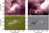 |
Fig. 1. Core dimming and brightenings. The core dimming in the southeast part of the erupting region as observed in the AIA 211 Å passband is depicted in panel a. The region bounded by the red rectangle in panel a is shown in panel b. The core dimming area is marked by the red dotted contour in panel b. An observation of the active region in the AIA 1600 Å passband is shown in panel c. Brightenings associated with the flare ribbons are marked by the blue contours. The radial component of the HMI vector magnetic field is plotted in grey scale with saturation values ±1000 G in panel d. The blue contours in panel d are the same as those plotted in panel c. The red contour in panel d denotes the boundary of the core dimming as marked in panel b. |
2.2. Models
2.2.1. TMFM model
We chose to use the data-driven and time-dependent magnetofrictional model (TMFM; Pomoell et al. 2019) to study the formation and early evolution of the FR. The simulation itself was carried out from 23 Dec. 2015 at 23:36 UT to 2 Jan. 2016 at 12:36 UT, with the simulation output analysed at a 6 h cadence (starting from 24 Dec. 2015 at 00:36 UT) with the simulation domain reaching a height of 200 Mm. The simulation was initialised with a potential magnetic field (for details, see Pomoell et al. 2019) using the first magnetogram of the sequence of maps as input. For the subsequent time-steps, photospheric electric field maps (electrograms) were derived from the time series of vector magnetograms (Lumme et al. 2017). These electograms drive the TMFM model, which computes the evolution of the coronal magnetic field using Faraday’s law, where the electric field is assumed to follow the resistive Ohm’s law. In contrast to MHD approaches, the velocity in the magnetofrictional model is explicitly obtained by setting it proportional to the Lorentz force (Yang et al. 1986; Pomoell et al. 2019):
 (1)
(1)
with ν being the magnetofrictional coefficient and μ0J = ∇ × B. With this prescription of the velocity, the system would relax towards a force-free state if the system were no longer driven by a net Poynting flux at the boundary. However, as the system is driven in a time-dependent manner, a force-free state is not reached. We selected a constant  , except at the lower photospheric boundary, where 1/ν smoothly approaches zero. The electric field at the boundary is decomposed such that it consists of an inductive and a non-inductive component. The former can be calculated straightforwardly from Faraday’s law:
  . The non-inductive component of the electric field, which originates from a scalar potential and is therefore not directly invertible from Faraday’s law, is computed using the method described in Lumme et al. (2017), as an optimisation problem. In this work, we use the optimised electrogram as determined in Price et al. (2020) based on optimising the calculated photospheric energy injection with the estimation given by the DAVE4VM method (Schuck 2008).
2.2.2. Zero-beta MHD modelling
The photospheric driving is a crucial element in the FR formation and destabilisation. However, once the FR begins to rise in the corona, it is likely that the lift-off continues even though the driving ceases. After this point, the photospheric boundary conditions should have only a minor effect on the modelled FR and its subsequent evolution. In this work, we switch off the driving at 29 Dec. 2015 at 6:36 UT, which is approximately 18 h after the observed M1.9 flare peak the previous day. The relatively long lag between the flare time and the ceasing of the driving is justified, because the coronal dynamics in TMFM simulations is slow by construction compared to typical eruptive timescales in the corona (e.g. Pomoell et al. 2019). Additionally, we evolve the resulting field configuration with a zero-beta MHD approach, as detailed in Daei et al. (2023). On the one hand, this is done to compare with the results of the magnetofrictional model (MFM) relaxation from Price et al. (2020). These authors stopped the driving at 12:00 on the 29 Dec. (i.e. only a few timesteps after our chosen relaxation time) and found that with MFM relaxation, the resulting FR is very similar to the fully driven TMFM FR. On the other hand, the zero-beta MHD relaxation may also counteract potential issues related to the slow evolution of the TMFM.
3. Flux-rope extraction algorithm and derivation of its key properties
To analyse the evolution of the FR in the simulations, we first identified it from a time series of data cubes containing the magnetic field information. This procedure is typically not straightforward. In this section, we first present our FR identification method and then explain how the footpoints of the FR and the enclosed magnetic flux are extracted from the simulation results. We also discuss the method we use to extract the footpoint dynamics and magnetic flux from observations.
3.1. Flux-rope extraction method
As FRs are commonly defined as structures, where a bundle of field lines wind around a common axis, they are expected to manifest as coherent, localised structures with high twist. Therefore, our FR extraction and tracking algorithm makes use of the twist number Tw, which is given by Liu et al. (2016) as:
 (2)
(2)
where J∥ is the component of the current density parallel to the magnetic field. The integral is evaluated along a given field line L. This quantity describes how many turns two infinitesimally close magnetic field lines make about each other.
The FR extraction scheme involves the following steps: First, we identify the last time instance, where the FR is still within the boundaries of the simulation domain. The identification is done by calculating Tw in a plane (cut along either x or y, cf. Fig. 2), which is chosen such that it captures the FR in all (relevant) time steps. Typically, a plane close to the polarity inversion line (PIL) of the region of interest fulfills this criterion. This procedure is carried out for all frames of the simulation. From these twist maps, we locate regions of high twist, which we define as Tw > 1 or Tw < −1 depending on the sign of the twist of the FR. The extraction and tracking is then performed from the selected time instance backwards. We count the extracted high-twist region as belonging to the same evolving structure if two subsequent regions overlap by at least 10%.
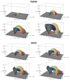 |
Fig. 2. Snapshots showing the evolution of the FRs. Snapshots are extracted from the TMFM simulation (normalised simulation times with respect to the flux evolution; see Sect. 3.4: 0.33, 0.63, 0.92, 1.21) and the MHD relaxation (normalised times: 0.86, 1.03, 1.19, 1.36) originating from AR12473, which is associated with the solar eruption on 28 Dec. 2015. The FR extraction method used an ϵ value of 0.03 in the TMFM case, and 0.04 for MHD (see text for details). The vertical magnetic field Bz at the photospheric boundary is shown at the bottom. Movies are available online. |
The tracked areas may appear quite irregular. Therefore, the shapes of the high-twist regions are reduced to circles as follows: First, the centroids of the extracted structures in the binary maps are calculated. The horizontal coordinates (i.e. either x or y – cf. Fig. 2 – depending on the orientation of the twist plane) of the centroids are averaged in time, in cases where the horizontal movement does not surpass 20 Mm during the evolution (excluding outliers). In cases of significant displacement, it is fitted with a second-order polynomial. In the event modelled here, the horizontal component stayed relatively stable for the TMFM case, while for the MHD simulation, it experienced significant displacement (> 30 Mm). The temporal evolution of the z coordinate is always fitted by a second-order polynomial. This approach avoids possible abrupt jumps in the evolution of the coordinates, as well as boundary effects, which occur when the FR approaches the walls of the simulation domain (e.g. deceleration).
The determination of the circle radius is based on the area of the extracted twisted structure as follows:
 (3)
(3)
where A is the area of the twisted region and ϵ is an empirical constant that quantifies the contribution from the highly twisted fields, which are not part of the FR itself (e.g. open field lines or field lines that connect to distinctly different regions on the photospheric boundary). The finite value of ϵ therefore results in a smaller FR radius than when setting ϵ to zero. κ is constrained for each time step by finding the value that gives the largest change in the average twist, which is the point where the curvature of the κ over twist per area graph is maximal. This approach is motivated by the assumption that the FR boundaries exhibit sharp changes in twist value. As the obtained ranges of κ can have a large scatter, the final values are determined by a linear fit to its temporal evolution.
As a last step, the value for ϵ is determined empirically based on the coherence and general appearance of the FR over time. To get an error estimate for the derived properties, the radius of the FR is calculated both with a non-zero, positive value and with ϵ set to zero. Having the centre and radius of the circle in 2D enables us to expand it to a sphere in 3D, where its surface is finally used to calculate the source points for the magnetic field lines of the FRs. Some snapshots of the extracted FRs for AR12473 are presented in Fig. 2.
3.2. Footpoint derivation from the simulation
The simulated footpoints of the FR are determined here as the intersecting points of the extracted field lines with the z = 0 plane, the photosphere. For the evolution and morphology analysis, uniform field line sampling was used with 100 points in longitude and latitude of the spherical source for each time step, which was derived following the methodology presented in Sect. 3.1. To capture the dynamics of the footpoints, we calculate their respective centroid and then determine the distance of both footpoint regions from this centroid.
3.3. Footpoint derivation from observations
As discussed in Sect. 1, the hooks of the J-shaped UV brightenings (ribbons) are expected to mark the FR footpoints. For the event presented here, the brightening areas do not extend to the presumed footpoint locations, but stay rather centrally on the inner edge of the two polarity regions (cf. Fig. 1). To extract the brightenings from the AIA 1600 Å maps, both base-difference and running-difference images have been created with a time cadence of 12 min. We created two base images from the average of the first two (28 Dec. 2015, at 10:59 UT and 11:11 UT) and the last two (28 Dec. 2015, at 13:35 UT and 13:47 UT) frames of the timeseries because the background conditions changed significantly during the event.
Regions that surpass a determined threshold (0.175, as found empirically to capture the main brightening area) in the difference maps are marked as brightening regions. We subsequently filter for small structures to get rid of noisy features in the resulting images. A binary mask outlining the extent of the ribbons over the time series is created. From this, we calculate the centroid of the ribbon structure, which is used as a reference point to estimate the movement of the brightening regions. This procedure is done for all three methods described above (base difference images using the starting frames, the final frames, and the running difference images). We then average the resulting distances from these three different methods (with respect to their respective centroid) and estimate the errors as their standard deviation. Finally, we want to track the movement of both brightening regions specifically in the frames where they appear as clear and significantly bright structures. We therefore only consider those frames where the average intensity of the AIA 1600 Å images is higher than their linear fit through the full time series.
Another observational signature of FR footpoints is a pair of core dimming regions in EUV images. For the studied event, only a single core dimming region was detected during the flare on 28 Dec. 2015 between 11:49 and 14:09 UT. We use base difference images in the AIA 211 Å pass band to manually extract the core dimming region as shown in panel b of Fig. 1; these were taken 10 min before the flare peak time. The core dimming can be seen at the southeast part of the active region. However, we do not observe a co-temporal counterpart of this core dimming region in the northwest, which is likely because it was obscured by the overlying arcade field lines on the northwest side of the active region. To capture the dimming dynamics, we add a flipped version of the dimming mask to artificially create a symmetric dimming structure. The movement of the dimming structure is then tracked (analogously to the brightenings and modelled footpoints) in reference to their respective centroid. We start our analysis with the time instance where the dimming becomes clearly identifiable (i.e. at 12:35 UT on 28 Dec. 2015).
To compare with our modelling results, the AIA images are projected to a 2D plane (assuming photospheric height levels), as our simulation domain is Cartesian. The evolution of both the EUV dimming regions and the UV brightenings is tracked and compared with the movement of the footpoints that are derived from the TMFM and the MHD relaxation run.
3.4. Toroidal flux calculation from the simulations
The footpoints derived from the model serve as the basis for calculation of toroidal flux. Here, it is calculated at the base of the simulation domain, that is, at the photospheric level by summing up ∑iBz, idA at the footpoint locations, where dA marks the area of the cells on the bottom boundary. This is done separately for both the positive and negative polarity footpoints. The resulting absolute fluxes from both regions are then averaged to obtain an estimation of the toroidal FR flux. As the TMFM and MHD simulation evolve on different timescales (also with respect to the actual eruption), we use the flux evolution of the TMFM simulations as a temporal reference and define a normalised time (τ) frame by setting the minimum in the TMFM toroidal flux curve to equal ‘time 0’ and the flux peak equal to ‘time 1’. The MHD normalised time is calibrated to match the TMFM normalised time at the initiation time, while its respective flux peak is also reached at time 1. We note that while the total flux in the FR is conserved, the contributions to it from toroidal and poloidal fluxes may change along the FR. We therefore average the toroidal fluxes from the positive and negative footpoints. Sampling-related uncertainties are also expected to have a small contribution.
3.5. Toroidal flux from observational data
We compared the toroidal flux evolution computed from the modelling to imaging observations by analysing the derived core dimming region (see Sect. 3.3). As only one core dimming was observed (see Sect. 3.2), we follow the approach by Xing et al. (2020), and compute the magnetic flux using this sole dimming region. Figure 1 depicts the outer boundary of the core dimming region, marked by the red dotted contour. Using the radial component (Br) data from an HMI vector magnetogram, the total magnetic flux within this boundary is determined by summing the flux (BrdA; dA is the area of a pixel in the HMI data) of each enclosed pixel. To avoid the noise in magnetic field data, we include only those pixels in our analysis where |Br|> 20 Gauss, following the threshold used by Wang et al. (2019) and Xing et al. (2020). In order to estimate the error associated with detecting the boundary of the core dimming area, we enlarge or reduce the identified dimming boundary (while keeping the contour shapes identical) to allow a 20% increase or decrease, respectively, in the enclosed area. This criteria of 20% change in boundary area is selected based on our manual inspection, where the aim is to ensure that the dimming boundary lies well within the prescribed error limit. We further estimate the associated change in underlying magnetic flux and assign this as the error in determining the toroidal flux.
4. Results
4.1. Flux rope evolution
The evolution of the extracted FR in the TMFM and the zero-beta MHD simulation are visualised in Fig. 2. The figure shows four snapshots from each model while the full evolution can be seen from the corresponding online movies. In addition, the height of the apex of the FR as a function of normalised simulation time τ for the two simulations is shown in Fig. 3. We remind that the zero-beta MHD simulation is a relaxation run (see Sect. 2.2.2) that was initialised with the TMFM snapshot on 29 Dec. 2015 at 6:36 UT. By this time, the FR had already formed in the TMFM simulation and risen about halfway through the simulation domain. The starting height of the FR in the zero-beta MHD is ∼130 Mm in the case of ϵ = 0 and ∼110 Mm in the case of ϵ = 0.04. The differences between the TMFM initialisation height and the MHD starting height are a result of inaccuracies of the extraction algorithm for individual time steps (see a brief discussion on this in Sect. 5.1).
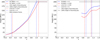 |
Fig. 3. Evolution of the height of the apex of the FR as extracted from the TMFM simulation (left panel) and from the zero-beta MHD relaxation (right panels). The blue dashed curve shows the results when applying the extraction scheme without ϵ prescription, while the red dashed curve depicts the FR height evolution with ϵ = 0.03 for the TMFM runs and ϵ = 0.04 for the MHD runs (see Sect. 3.1). The x-axis depicts the time normalised to the TMFM flux evolution (Sect. 3.4). The horizontal lines show 10% (grey) and 100% (black) of the domain height. The dotted vertical lines indicate the start- and endpoints of our analysis with (red) and without ϵ-prescription (blue), as described in Sect. 4.1. |
The FR computed with the TMFM (top panels of Fig. 2) evolves very coherently and smoothly through the simulation domain until the height limit of 200 Mm. The FR can be visually divided into two distinct parts, illustrated with reddish-beige and blueish field lines. The structure depicted by the blueish field lines warps around the reddish-beige structure. The orientation of the field in the figure is such that the left-hand footpoint corresponds to the negative polarity one. The left panel of Fig. 3 also demonstrates that while the FR evolves very smoothly overall through the low corona, the rate at which it rises increases approximately 100 Mm above the photosphere. This occurs at the simulation frame corresponding to 29 Dec. 00:36 UT, which is one frame (i.e. 6 h) before the snapshot used to initiate the zero-beta MHD relaxation run.
The zero-beta MHD FR (bottom panels of Fig. 2) has a relatively similar appearance to the TMFM FR overall; it is coherent and features similar structures, with the blueish field lines again wrapping around the reddish-beige ones. The most notable differences are the tube radius, height evolution, and the amount of twist, particularly of the blueish field lines. In the later stages, the MHD FR appears significantly thinner, which applies to both bluish and reddish-beige structures.
After initialisation of the zero-beta MHD simulation, it takes some time for the FR to begin rising. The FR then rises at a steady rate –but slower than in the TMFM simulation– in our normalised time units. When the point is reached where boundary effects are expected to start to affect the evolution, the rate of rise decreases (see Fig. 3). In contrast to the TMFM simulation, the apex of the FR does not reach the top of the simulation box but approaches it slowly. The slower rise and deceleration of the rise at the end of the simulation for the MHD FR may be due to the FR approaching and interacting with the upper domain boundary (for more details, see the Discussion in Sect. 5). Therefore, we exclude both the initial and end phases of the FR evolution from the subsequent analysis for the zero-beta MHD results based on a velocity threshold (see vertical lines in Fig. 3).
4.2. Footpoint analysis
The derived footpoint movement is detailed in Fig. 4 following the methodology introduced in Sect. 3.3. The plots show the distances of both positive and negative polarity footpoints and features from their respective centroid as a function of time.
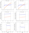 |
Fig. 4. Distance of the footpoint or feature location from its respective centroid for footpoints from TMFM and MHD, as well as brightenings and dimmings. The x-axis depicts the normalised time τ (see Sect. 3.4). Orange: western footpoint (positive polarity) region. Blue: eastern footpoint (negative polarity) region. In the top two panels, the pair of vertical lines shows the frames when the apex of the FR was between 10% and 100% of the simulation box. For the MHD results in the middle panel, we used a velocity threshold to identify relevant frames (cf. Fig. 3). For the brightening and dimming time window, we followed the steps presented in Sect. 3.3. |
We created linear fits through the relevant data points (as discussed in Sects. 3.3 and 4.1) and calculated the average movement of the footpoints or observational features with respect to their centroid locations. The resulting slopes of the linear fits are shown in Table 1. We note that only one dimming region, located in the eastern negative polarity part, was clearly identifiable; see Sect. 3.3 for details.
The faster movement of the positive-polarity footpoint regions (orange dots in Fig. 4; i.e. western footpoints) is clearly visible for both simulations and the brightenings. For both simulations, the negative-polarity footpoint region (blue dots, i.e. eastern footpoints) is relatively stable when compared to the positive-polarity footpoints. In both TMFM and MHD cases, the footpoints move away from their centroid; they recede from each other as the simulation progresses. Even after the FR in the MHD simulation starts to decelerate (i.e. falls below a velocity threshold), the trend for the positive-polarity footpoint continues.
The previously described behaviour found in the simulated footpoint dynamics is less clear for the brightenings, which may be due to the limited number of data points. The movement is also generally more erratic. However, the positive polarity region exhibits both stronger dynamics and a positive slope, which is similar to simulation results. On the contrary, the negative polarity brightening shows a negative slope. The movement of the core dimming in the negative polarity region in the 211 Å AIA channel agrees exceptionally well with the respective brightening results and the value of the slope is very similar; cf. Table 1.
4.3. Toroidal flux analysis
The results of the computation of the toroidal magnetic flux enclosed in the FR (for details, see Sect. 3.4) are presented in Fig. 5. Similarly to the footpoint analysis, for the TMFM FR, the time interval is shown when the FR height is between 10% and 100% of the domain height, while for the MHD FR, a velocity threshold of 1 Mm per time step has to be reached.
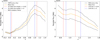 |
Fig. 5. FR flux in the TMFM simulation as well as the zero-beta MHD simulation for the same event, with the normalised time τ on the x-axis (see Sect. 3.4). The red and blue pairs of dashed lines indicate the start and endpoints of the most relevant frames for the simulated FRs with and without taking ϵ into account, respectively. The dashed grey line in the TMFM plot indicates the initiation time for the zero-beta MHD simulation. |
The TMFM FR shows a nearly monotonous increase in toroidal flux until the FR approaches the top boundary of the simulation domain. After reaching the top (or shortly before in the case of the ϵ = 0.03 FR), the flux begins to decline. For the MHD FR, the flux first decreases before it increases towards the peak value (we note that we consider here only times where the velocity limit was satisfied). After reaching this maximum, the flux declines steadily. Contrary to the TMFM FR, this decline already sets in, when boundary conditions should not yet play a role in the FR evolution.
The flux derived from the core dimming observation in 211 Å is shown in Fig. 6 together with the dimming area and the GOES light curve. We were not able to capture the rising phase observed in the model results, but a clear declining phase matches especially well with the MHD results.
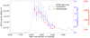 |
Fig. 6. Temporal evolution of the toroidal flux and the core-dimming area. The black curve denotes the co-temporal evolution of the GOES soft X-ray flux. |
5. Discussion
5.1. Flux-rope extraction discussion
The developed semi-automated extraction of the FR from the simulation data is highly beneficial for studies of the early dynamics and evolution of FRs. The method uses a twist threshold (here twist number |Tw|> 1), a requirement of coherency of the rising structure, and constraints of a circular cross-section in a plane close to the polarity inversion line. The radius of the circle was determined by finding the value that gives the largest change in the average twist.
However, there are some steps in the extraction procedure that may affect the outcome of the analysis. Firstly, the twist threshold may influence the extent of the extracted FR and therefore the centroid of the FR structure. However, the radius of the source sphere itself is only weakly dependent on the twist threshold, as the κ (Eq. (3)) is ultimately responsible for setting the source radius. κ therefore counteracts possible non-optimal thresholds for the twist map, as long as they are in a reasonable range. Secondly, FR cross-sections may also deviate significantly from circular shapes (Price et al. 2020; Kilpua et al. 2021). Furthermore, as we use fitting procedures over the whole simulation time to smooth the centroid and radius evolution of the FR, individual frames may not completely capture the FR at a given time instance. This explains why in our simulation the MHD FR at the initiation time had quite different toroidal flux (cf. Fig. 5) and height values (cf. Fig. 3) compared to the TMFM FR.
Furthermore, here we use a version of the twist number (Tw) that describes the number of turns a field line takes around an infinitesimally close field line (Liu et al. 2016). This is therefore different from the general definition of the FR as a structure where field lines wind about a common axis. In this regard, a more accurate approach would have been to use the twist number Tg, which is defined as the number of turns a field line takes about a defined (FR) axis (e.g. Liu et al. 2016; Price et al. 2022; Berger & Prior 2006; Guo et al. 2017). However, computation of the FR axis is non-trivial and the procedure requires knowledge of Tw (Price et al. 2022). Therefore, we decided that the most feasible approach for automated flux rope identification is to use Tw instead of Tg.
We incorporated a correction parameter (ϵ) to reduce the amount of highly twisted surrounding field that has distinctly different topology and/or connectivity at the photospheric level. While the ϵ parameter may be very effective in removing unwanted field lines, it also comes with trade-offs: The surrounding non-FR field lines are most of the time not equally distributed around the FR boundaries, and therefore reducing the circular cross section of the twisted structure cuts out actual FR field lines too. It is for this reason that we computed the height, footpoints, and flux evolutions both with and without the ϵ prescription. This also helps us to obtain an error estimation. We used a fixed value for this correction parameter, but it could be modified to incorporate a time dependence in the future.
Figure 7 showcases the effect of applying ϵ to the FR. The removal of field lines that connect to different regions in the photosphere from those in the main FR can be seen clearest in the later stages of the simulations (bottom panels for both TMFM and MHD). We note that a significant number of excluded blue field lines blend in well with the main FR.
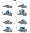 |
Fig. 7. Example FR field lines from the extraction method with ϵ prescription (white) and without (blue) for the TMFM and the MHD relaxation simulation. The frames are the same as in Fig. 2. |
The results of the footpoint derivation and especially the flux calculation may also be affected by the inclusion of magnetic field lines that exit the side walls of the simulation domain. However, for these simulations, their contribution was minimal (some can be seen in the bottom panels for the MHD run in Fig. 2).
5.2. Modelling discussion
In this work, we applied the extraction method for two simulations: (1) a TMFM simulation and (2) a relaxation run, which uses a zero-beta MHD model (Daei et al. 2023) that was initiated using a TMFM snapshot approximately halfway through the TMFM simulation without any additional driving after this point. The exact relaxation time of 29 Dec. 2015 at 6:36 UT yielded an erupting FR, which is consistent with the magnetofrictional relaxation carried out by Price et al. (2020).
The extracted FRs generally agree well with the common perception of a magnetic FR; they feature a coherent and gradually rising structure, containing twisted field lines winding about a shared axis. We find that the MHD FR deviates slightly more from its original coherence in the later stages than the TMFM FR (cf. Fig. 2). Furthermore, the rise of the MHD FR decelerates and it remains within the domain throughout the entire simulation. It must be noted that this is most likely a boundary effect and not the FR finding an actual new equilibrium. We therefore restricted our analysis to those frames where the MHD FR was rising sufficiently fast (at a velocity of at least 1 Mm per time step). This requirement also excluded the very early phase where the instability of the FR is slowly building up. The TMFM FR evolution is limited by reaching 10% (lower limit) and 100% (upper limit) of the height of the simulation domain. Within their respective boundaries, the appearance and dynamics of the TMFM and MHD FRs seem to agree well with each other, both in terms of general morphology and temporal evolution.
5.3. Footpoints and toroidal flux
The footpoint movement as deduced from the modelling and the observational analysis (i.e. from the dimming and brightenings) generally agree well with each other. However, there are some differences in the dynamics; for example, the speed with which footpoints recede from the common centroid. This is presumably due to the fact that the observational proxies cover only some particular phase of the FR evolution, while in the simulation, the FR can be tracked until it reaches the top of the domain or boundary effects start to interfere. Furthermore, the movement of the negative polarity footpoint region in observations is directed towards the respective centroid, contrary to the modelling results. However, we remind the reader that the movement of the negative polarity footpoint is relatively minor when compared to the evolution of the positive polarity region and therefore no strong conclusions can be drawn. The observational features may also partly capture other parts of the FR system apart from the footpoints. As discussed in Sect. 1, the UV brightenings can be complex and reflect interplay between the FR fields and surrounding arcade fields. Although the evolution of the brightenings should correlate with the movement of the footpoints during the eruption, they provide information about the current sheets related to the erupting structure, rather than about the footpoints directly. The generally different underlying effects can also be understood when observing that the relevant time windows for the brightenings and dimming are shifted by 30 min with respect to each other. We note that the slopes for the negative polarity regions derived from dimming and brightenings match exceptionally well, suggesting that they have both captured the same kind of moving structure. The trend of the footpoints receding from the centroid is generally evident both from the simulated and the observed data in the very dynamic, positive polarity footpoint region. The dynamics of the positive-polarity footpoint region are present in both the simulation and the brightenings. However, the behaviour of the dynamics is not reliably captured by the dimming analysis, because we do not observe any dimmings in this particular region. The derived slopes (see Sect. 1) summarise these trends, though their magnitude differs notably between the simulation and observational features due to different timescales, as discussed above.
We find that, for the simulated FRs within their respective restricted time windows, the toroidal flux first increases steadily. After reaching its peak, we observe a declining trend, which is especially pronounced in the MHD case. The decline in toroidal flux sets in rather late for the TMFM FR, when it approaches the domain boundary. However, we cannot draw strong conclusions after the time when the FR begins to exit the simulation domain as this directly reduces the flux.
The two-phase evolution of toroidal flux that we see in simulations is consistent with the observational investigation by Xing et al. (2020). In our case, we could only capture the declining phase from observations, that is, from the core-dimming analysis (see Fig. 6). This could also be due to the fact that the dimming evolution was not clearly trackable in the beginning phase of the flare. Xing et al. (2020) speculate that the two-phase evolution of the toroidal flux is caused by the flux first increasing as the FR quickly forms by reconnection with the overlying field. Subsequently, the decrease sets in due to reconnection between the twisted fields within the FR, converting toroidal to poloidal fields.
6. Conclusion
We developed a semi-automatic extraction algorithm to track eruptive coronal FRs in data-driven simulations. The method was applied to the active region AR12473 using both the time-dependent magnetofrictional method (TMFM) and a zero-beta MHD relaxation approach. Both simulations result in an erupting FR. We determined the evolution of toroidal magnetic flux and the footpoint movement from the simulations and compared these with the coronal brightenings and dimmings. We find that, during the eruption process, the modelled FR footpoints, the brightenings, and the dimmings move away from their respective central location, and that this movement is more pronounced for the positive-polarity region. The resulting trends are summarised in Table 1. The derived toroidal magnetic FR flux through the modelled footpoints shows a two-phase evolution: a rising and then a declining phase, which is most clear in the MHD case. Our observational investigation shows mostly a decline in toroidal flux, though we may not be capturing the build up of flux, as this may have happened before the dimmings became observable.
Our study shows that the algorithm we have developed can successfully capture the early dynamics of the FR and derive the evolution of some of its key properties. This tracking method also facilitates the statistical analysis of simulated FRs and can be used to tracking the evolution of their parameters. Refining the FR extraction method and applying it to investigate other aspects of FR eruptions could be an avenue for future research as well.
Movies
Movie 1 associated with Fig. 2 (MHD_Relaxation_Animation_Fig2) Access Supplementary Material
Movie 2 associated with Fig. 2 (TMFM_Animation_Fig2) Access Supplementary Material
Acknowledgments
SDO data are courtesy of NASA/SDO and the AIA and HMI science teams. This research has made use of NASA’s Astrophysics Data System. Furthermore, to compute and visualize the flux ropes, the open source python visualization tool VisIt (Childs et al. 2012) was used, as well as the PyVista package for multiple applications within this paper (Sullivan & Kaszynski 2019). This project has received funding from the European Union’s Horizon 2020 research and innovation programme under the Marie Skłodowska-Curie grant agreement No. 955620. S.P. acknowledges support from the projects C14/19/089 (C1 project Internal Funds KU Leuven), G.0B58.23N (FWO-Vlaanderen), SIDC Data Exploitation (ESA Prodex-12), and Belspo project B2/191/P1/SWiM. E.K.J.K., A.K. and F.D. acknowledge the ERC under the European Union’s Horizon 2020 Research and Innovation Programme Project SolMAG 724391, and Academy of Finland Project 310445. R.S. acknowledges support from the project EFESIS (Exploring the Formation, Evolution and Space-weather Impact of Sheath-regions) under the Academy of Finland Grant 350015. J.P and F.D. acknowledge Academy of Finland project 343581. All UH authors acknowledge the Finnish Centre of Excellence in Research of Sustainable Space (Academy of Finland grant numbers 312390, 312357, 312351 and 336809).
References
- Attrill, G., Nakwacki, M. S., Harra, L. K., et al. 2006, Sol. Phys., 238, 117 [Google Scholar]
- Aulanier, G., & Dudík, J. 2019, A&A, 621, A72 [NASA ADS] [CrossRef] [EDP Sciences] [Google Scholar]
- Berger, M. A., & Prior, C. 2006, J. Phys. A Math. Gen., 39, 8321 [Google Scholar]
- Chen, J. 2017, Phys. Plasmas, 24, 090501 [Google Scholar]
- Cheng, J. X., & Qiu, J. 2016, ApJ, 825, 37 [NASA ADS] [CrossRef] [Google Scholar]
- Cheung, M. C. M., & DeRosa, M. L. 2012, ApJ, 757, 147 [NASA ADS] [CrossRef] [Google Scholar]
- Childs, H., Brugger, E., Whitlock, B., et al. 2012, High Performance Visualization–Enabling Extreme-Scale Scientific Insight, 357 [Google Scholar]
- Couvidat, S., Schou, J., Hoeksema, J. T., et al. 2016, Sol. Phys., 291, 1887 [Google Scholar]
- Daei, F., Pomoell, J., Price, D. J., et al. 2023, A&A, 676, A141 [NASA ADS] [CrossRef] [EDP Sciences] [Google Scholar]
- Démoulin, P., Priest, E. R., & Lonie, D. P. 1996, J. Geophys. Res., 101, 7631 [Google Scholar]
- Dissauer, K., Veronig, A. M., Temmer, M., Podladchikova, T., & Vanninathan, K. 2018, ApJ, 855, 137 [NASA ADS] [CrossRef] [Google Scholar]
- Green, L. M., Török, T., Vršnak, B., Manchester, W., & Veronig, A. 2018, Space Sci. Rev., 214, 46 [Google Scholar]
- Guo, Y., Pariat, E., Valori, G., et al. 2017, ApJ, 840, 40 [NASA ADS] [CrossRef] [Google Scholar]
- Janvier, M., Aulanier, G., Bommier, V., et al. 2014, ApJ, 788, 60 [Google Scholar]
- Kilpua, E. K. J., Lugaz, N., Mays, M. L., & Temmer, M. 2019, Space Weather, 17, 498 [NASA ADS] [CrossRef] [Google Scholar]
- Kilpua, E. K. J., Pomoell, J., Price, D., Sarkar, R., & Asvestari, E. 2021, Front. Astron. Space Sci., 8, 35 [NASA ADS] [CrossRef] [Google Scholar]
- Lemen, J. R., Title, A. M., Akin, D. J., et al. 2012, Sol. Phys., 275, 17 [Google Scholar]
- Liu, R., Kliem, B., Titov, V. S., et al. 2016, ApJ, 818, 148 [Google Scholar]
- Lowder, C., & Yeates, A. 2017, ApJ, 846, 106 [Google Scholar]
- Lumme, E., Pomoell, J., & Kilpua, E. K. J. 2017, Sol. Phys., 292, 191 [CrossRef] [Google Scholar]
- Mackay, D. H., Green, L. M., & van Ballegooijen, A. 2011, ApJ, 729, 97 [NASA ADS] [CrossRef] [Google Scholar]
- Mandrini, C. H., Pohjolainen, S., Dasso, S., et al. 2005, A&A, 434, 725 [NASA ADS] [CrossRef] [EDP Sciences] [Google Scholar]
- Mandrini, C. H., Nakwacki, M. S., Attrill, G., et al. 2007, Sol. Phys., 244, 25 [NASA ADS] [CrossRef] [Google Scholar]
- Moore, R. L., Larosa, T. N., & Orwig, L. E. 1995, ApJ, 438, 985 [NASA ADS] [CrossRef] [Google Scholar]
- Palmerio, E., Kilpua, E. K. J., James, A. W., et al. 2017, Sol. Phys., 292, 39 [Google Scholar]
- Pesnell, W. D., Thompson, B. J., & Chamberlin, P. C. 2012, Sol. Phys., 275, 3 [Google Scholar]
- Pomoell, J., Lumme, E., & Kilpua, E. 2019, Sol. Phys., 294, 41 [NASA ADS] [CrossRef] [Google Scholar]
- Price, D. J., Pomoell, J., Lumme, E., & Kilpua, E. K. J. 2019, A&A, 628, A114 [NASA ADS] [CrossRef] [EDP Sciences] [Google Scholar]
- Price, D. J., Pomoell, J., & Kilpua, E. K. J. 2020, A&A, 644, A28 [NASA ADS] [CrossRef] [EDP Sciences] [Google Scholar]
- Price, D. J., Pomoell, J., & Kilpua, E. K. J. 2022, Front. Astron. Space Sci., 9, 1076747 [CrossRef] [Google Scholar]
- Schou, J., Scherrer, P. H., Bush, R. I., et al. 2012, Sol. Phys., 275, 229 [Google Scholar]
- Schuck, P. W. 2008, ApJ, 683, 1134 [NASA ADS] [CrossRef] [Google Scholar]
- Sullivan, C. B., & Kaszynski, A. 2019, J. Open Sour. Softw., 4, 1450 [NASA ADS] [CrossRef] [Google Scholar]
- Thompson, B. J., Plunkett, S. P., Gurman, J. B., et al. 1998, Geophys. Res. Lett., 25, 2465 [Google Scholar]
- Titov, V. S., Hornig, G., & Démoulin, P. 2002, J. Geophys. Res.: Space Physics, 107, 1164 [Google Scholar]
- Veronig, A. M., Gömöry, P., Dissauer, K., Temmer, M., & Vanninathan, K. 2019, ApJ, 879, 85 [NASA ADS] [CrossRef] [Google Scholar]
- Wang, W., Zhu, C., Qiu, J., et al. 2019, ApJ, 871, 25 [NASA ADS] [CrossRef] [Google Scholar]
- Webb, D. F., Lepping, R. P., Burlaga, L. F., et al. 2000, J. Geophys. Res., 105, 27251 [NASA ADS] [CrossRef] [Google Scholar]
- Xing, C., Cheng, X., & Ding, M. D. 2020, The Innovation, 1, 100059 [NASA ADS] [CrossRef] [Google Scholar]
- Yang, W. H., Sturrock, P. A., & Antiochos, S. K. 1986, ApJ, 309, 383 [NASA ADS] [CrossRef] [Google Scholar]
- Zemanová, A., Dudík, J., Aulanier, G., Thalmann, J. K., & Gömöry, P. 2019, ApJ, 883, 96 [Google Scholar]
All Tables
All Figures
|
Fig. 1. Core dimming and brightenings. The core dimming in the southeast part of the erupting region as observed in the AIA 211 Å passband is depicted in panel a. The region bounded by the red rectangle in panel a is shown in panel b. The core dimming area is marked by the red dotted contour in panel b. An observation of the active region in the AIA 1600 Å passband is shown in panel c. Brightenings associated with the flare ribbons are marked by the blue contours. The radial component of the HMI vector magnetic field is plotted in grey scale with saturation values ±1000 G in panel d. The blue contours in panel d are the same as those plotted in panel c. The red contour in panel d denotes the boundary of the core dimming as marked in panel b. |
| In the text | |
|
Fig. 2. Snapshots showing the evolution of the FRs. Snapshots are extracted from the TMFM simulation (normalised simulation times with respect to the flux evolution; see Sect. 3.4: 0.33, 0.63, 0.92, 1.21) and the MHD relaxation (normalised times: 0.86, 1.03, 1.19, 1.36) originating from AR12473, which is associated with the solar eruption on 28 Dec. 2015. The FR extraction method used an ϵ value of 0.03 in the TMFM case, and 0.04 for MHD (see text for details). The vertical magnetic field Bz at the photospheric boundary is shown at the bottom. Movies are available online. |
| In the text | |
|
Fig. 3. Evolution of the height of the apex of the FR as extracted from the TMFM simulation (left panel) and from the zero-beta MHD relaxation (right panels). The blue dashed curve shows the results when applying the extraction scheme without ϵ prescription, while the red dashed curve depicts the FR height evolution with ϵ = 0.03 for the TMFM runs and ϵ = 0.04 for the MHD runs (see Sect. 3.1). The x-axis depicts the time normalised to the TMFM flux evolution (Sect. 3.4). The horizontal lines show 10% (grey) and 100% (black) of the domain height. The dotted vertical lines indicate the start- and endpoints of our analysis with (red) and without ϵ-prescription (blue), as described in Sect. 4.1. |
| In the text | |
|
Fig. 4. Distance of the footpoint or feature location from its respective centroid for footpoints from TMFM and MHD, as well as brightenings and dimmings. The x-axis depicts the normalised time τ (see Sect. 3.4). Orange: western footpoint (positive polarity) region. Blue: eastern footpoint (negative polarity) region. In the top two panels, the pair of vertical lines shows the frames when the apex of the FR was between 10% and 100% of the simulation box. For the MHD results in the middle panel, we used a velocity threshold to identify relevant frames (cf. Fig. 3). For the brightening and dimming time window, we followed the steps presented in Sect. 3.3. |
| In the text | |
|
Fig. 5. FR flux in the TMFM simulation as well as the zero-beta MHD simulation for the same event, with the normalised time τ on the x-axis (see Sect. 3.4). The red and blue pairs of dashed lines indicate the start and endpoints of the most relevant frames for the simulated FRs with and without taking ϵ into account, respectively. The dashed grey line in the TMFM plot indicates the initiation time for the zero-beta MHD simulation. |
| In the text | |
|
Fig. 6. Temporal evolution of the toroidal flux and the core-dimming area. The black curve denotes the co-temporal evolution of the GOES soft X-ray flux. |
| In the text | |
|
Fig. 7. Example FR field lines from the extraction method with ϵ prescription (white) and without (blue) for the TMFM and the MHD relaxation simulation. The frames are the same as in Fig. 2. |
| In the text | |
Current usage metrics show cumulative count of Article Views (full-text article views including HTML views, PDF and ePub downloads, according to the available data) and Abstracts Views on Vision4Press platform.
Data correspond to usage on the plateform after 2015. The current usage metrics is available 48-96 hours after online publication and is updated daily on week days.
Initial download of the metrics may take a while.