| Issue |
A&A
Volume 644, December 2020
|
|
|---|---|---|
| Article Number | A163 | |
| Number of page(s) | 27 | |
| Section | Cosmology (including clusters of galaxies) | |
| DOI | https://doi.org/10.1051/0004-6361/202038219 | |
| Published online | 15 December 2020 | |
HOLISMOKES
II. Identifying galaxy-scale strong gravitational lenses in Pan-STARRS using convolutional neural networks⋆
1
Max-Planck-Institut für Astrophysik, Karl-Schwarzschild-Str. 1, 85748 Garching, Germany
e-mail: rcanameras@mpa-garching.mpg.de
2
Physik Department, Technische Universität München, James-Franck Str. 1, 85741 Garching, Germany
3
Institute of Astronomy and Astrophysics, Academia Sinica, 11F of ASMAB, No. 1, Section 4, Roosevelt Road, Taipei 10617, Taiwan
4
Technical University of Munich, Department of Informatics, Boltzmann-Str. 3, 85748 Garching, Germany
5
Institute of Physics, Laboratory of Astrophysics, Ecole Polytechnique Fédérale de Lausanne (EPFL), Observatoire de Sauverny, 1290 Versoix, Switzerland
Received:
21
April
2020
Accepted:
4
June
2020
We present a systematic search for wide-separation (with Einstein radius θE ≳ 1.5″), galaxy-scale strong lenses in the 30 000 deg2 of the Pan-STARRS 3π survey on the Northern sky. With long time delays of a few days to weeks, these types of systems are particularly well-suited for catching strongly lensed supernovae with spatially-resolved multiple images and offer new insights on early-phase supernova spectroscopy and cosmography. We produced a set of realistic simulations by painting lensed COSMOS sources on Pan-STARRS image cutouts of lens luminous red galaxies (LRGs) with redshift and velocity dispersion known from the sloan digital sky survey (SDSS). First, we computed the photometry of mock lenses in gri bands and applied a simple catalog-level neural network to identify a sample of 1 050 207 galaxies with similar colors and magnitudes as the mocks. Second, we trained a convolutional neural network (CNN) on Pan-STARRS gri image cutouts to classify this sample and obtain sets of 105 760 and 12 382 lens candidates with scores of pCNN > 0.5 and > 0.9, respectively. Extensive tests showed that CNN performances rely heavily on the design of lens simulations and the choice of negative examples for training, but little on the network architecture. The CNN correctly classified 14 out of 16 test lenses, which are previously confirmed lens systems above the detection limit of Pan-STARRS. Finally, we visually inspected all galaxies with pCNN > 0.9 to assemble a final set of 330 high-quality newly-discovered lens candidates while recovering 23 published systems. For a subset, SDSS spectroscopy on the lens central regions proves that our method correctly identifies lens LRGs at z ∼ 0.1–0.7. Five spectra also show robust signatures of high-redshift background sources, and Pan-STARRS imaging confirms one of them as a quadruply-imaged red source at zs = 1.185, which is likely a recently quenched galaxy strongly lensed by a foreground LRG at zd = 0.3155. In the future, high-resolution imaging and spectroscopic follow-up will be required to validate Pan-STARRS lens candidates and derive strong lensing models. We also expect that the efficient and automated two-step classification method presented in this paper will be applicable to the ∼4 mag deeper gri stacks from the Rubin Observatory Legacy Survey of Space and Time (LSST) with minor adjustments.
Key words: gravitational lensing: strong / methods: data analysis / galaxies: distances and redshifts / surveys
Full Table 1 is only available at the CDS via anonymous ftp to cdsarc.u-strasbg.fr (130.79.128.5) or via http://cdsarc.u-strasbg.fr/viz-bin/cat/J/A+A/644/A163
© R. Cañameras et al. 2020
 Open Access article, published by EDP Sciences, under the terms of the Creative Commons Attribution License (https://creativecommons.org/licenses/by/4.0), which permits unrestricted use, distribution, and reproduction in any medium, provided the original work is properly cited.
Open Access funding provided by Max Planck Society.
1. Introduction
Strongly lensed systems with time-variable sources provide competitive probes of the Hubble constant H0, which are independent of cosmic microwave background (CMB) observations (Planck Collaboration VI 2020) and the local distance ladder (Riess et al. 2019; Freedman et al. 2019, 2020), and allow one to assess the significance of the current H0 tension. The COSmological MOnitoring of GRAvitational Lenses (COSMOGRAIL) and H0 Lenses in COSMOGRAIL’s Wellspring (H0LiCOW) projects (e.g., Suyu et al. 2017; Courbin et al. 2018) have recently established the capacity of combining time-delay measurements and robust strong lensing models to constrain H0 and measured  km s−1 Mpc−1 in flat Lambda cold dark matter (ΛCDM) cosmology using six lensed quasars (Wong et al. 2020). The seventh lens has been analyzed by the STRong lensing Insights into the Dark Energy Survey (STRIDES) collaboration (Shajib et al. 2020; Buckley-Geer et al. 2020), and a detailed study of systematic effects is presented by Millon et al. (2020) as part of the Time-Delay COSMOgraphy (TDCOSMO) organization. Moreover, the first two strongly lensed supernovae (SNe) with spatially-resolved multiple images have been detected in recent years; one core-collapse SN was found behind the strong lensing cluster MACS J1149.5+222.3 (SN Refsdal, Kelly et al. 2015), and one type Ia SN was found behind an isolated lens galaxy (iPTF16geu, Goobar et al. 2017). These findings open new perspectives on future H0 measurements with lensed SNe. These types of systems are indeed well-suited for time-delay measurements given the smooth, nonerratic SNe light curves which require shorter high-cadence monitoring than lensed quasars, and the possibility of reducing microlensing effects by focusing on the early, achromatic expansion phase a few weeks after explosion, and by using color light curves (Suyu et al. 2020; Huber et al. 2019, and in prep.; Bonvin et al. 2019; Goldstein et al. 2018). For lensed type Ia SNe, the standardizable intrinsic peak luminosity of the source is also a valuable input for breaking the mass-sheet degeneracy in lens mass models (Falco et al. 1985). Constraints on H0 have already been derived with SN Refsdal (Grillo et al. 2018, 2020) and they illustrate the great potential of such measurements, in particular for galaxy-scale strong lens systems that have simpler lens mass distributions than galaxy clusters. Lensed SNe with adequate image separations providing time delays of a few days to weeks are particularly promising and are relatively less sensitive to microlensing effects (Suyu et al. 2020; Huber et al. 2019).
In addition to precise measurements of the Hubble constant, strongly lensed SNe are promising as they allow for early-phase SN studies. Multiply-imaged SNe detected from the first image can be combined with strong lensing models to predict the time delays and future SN reappearance, as was done for SN Refsdal, in order to trigger follow-up observations within a few days of explosion. This is currently not feasible for unlensed SNe beyond the local Universe due to their late discovery near peak luminosity. Such early-phase studies are particularly valuable when tackling the progenitor problem of type Ia SNe and disentangling the single-degenerate (Whelan & Iben 1973), double-degenerate (Tutukov & Yungelson 1981), and additional scenarios that have been extensively debated over the last decades. For core-collapse SNe, these observations are important in order to characterize the progenitor properties and compare them with current stellar evolution models. Early-phase spectroscopy of type II SNe would yield novel constraints on the mass-loss history just before explosion.
We recently initiated the Highly Optimized Lensing Investigations of Supernovae, Microlensing Objects, and Kinematics of Ellipticals and Spirals (HOLISMOKES, Suyu et al. 2020) program to address these fundamental questions on stellar physics and cosmology. The number of strongly lensed SNe is expected to grow over the next few years, thanks to the on-going Zwicky Transient Facility (ZTF, Masci et al. 2019) high-cadence survey on the Northern Hemisphere and the forthcoming Rubin Observatory Legacy Survey of Space and Time (LSST, Ivezić et al. 2019) on the South. Oguri & Marshall (2010) predict 45 strongly lensed type Ia SNe over the ten years of LSST, which corresponds to a few events for the shallower ZTF survey. This assumes a selection from spatially-resolved multiple images targeting the most useful wide-separation systems. Using complementary selection techniques solely based on magnification of SN Ia light curves, Goldstein & Nugent (2017) predict ten to 20 times more lensed SN Ia albeit mostly with small image separations (see also Wojtak et al. 2019). Importantly, new lensed SNe candidates have to be selected early enough to start the follow-up sequence in a timely manner. One way is to extend the numerous, successful searches of galaxy-scale strong lenses that were traditionally conducted on surveys with optimal image quality (e.g., More et al. 2016; Sonnenfeld et al. 2018), to surveys with largest sky coverage, in order to quickly identify transients matching the position of background lensed sources. Ultimately, these lens finding pipelines will be directly applicable to the deep LSST stacks which are expected to yield approximately a hundred thousand new systems (Collett 2015).
Galaxy-scale strong gravitational lenses without time-variable sources also provide valuable insights into the lens total mass distributions, including the inner dark-matter fractions (e.g., Gavazzi et al. 2007; Grillo et al. 2009; Sonnenfeld et al. 2015; Schuldt et al. 2019), the slopes of the total and dark-matter mass density profiles (e.g., Treu & Koopmans 2002; Koopmans et al. 2009; Barnabè et al. 2011; Shu et al. 2015), and the spatial extent of dark-matter halos (e.g., Halkola et al. 2007; Suyu & Halkola 2010). Such systems play a crucial role in characterizing the lens stellar initial mass function (IMF), a major ingredient for stellar mass estimates, as a function of galaxy physical properties (e.g., Cañameras et al. 2017a; Barnabè et al. 2013; Sonnenfeld et al. 2019), and they are well-suited to search for dark-matter substructures (e.g., Vegetti et al. 2012; Hezaveh et al. 2016; Ritondale et al. 2019). Moreover, high magnification factors provide unique diagnostics on the local interstellar medium physical conditions in lensed high-redshift galaxies and on the local feedback mechanisms driving their evolution (e.g., Danielson et al. 2011; Cañameras et al. 2017b; Cava et al. 2018).
Strong lensing events are rare, about one in 1000 for high-resolution space-based imaging (e.g., Marshall et al. 2009) and down to about one in 105 for seeing-limited ground-based data (e.g., Jacobs et al. 2019a). Thus, their identification requires dedicated and automated methods. For instance, arc-finder algorithms (e.g., Gavazzi et al. 2014; Sonnenfeld et al. 2018) and citizen-science classification projects (SPACE WARPS, Marshall et al. 2016) have been developed over the last decade. In particular, convolutional neural networks (CNNs) are supervised machine-learning algorithms optimized to image analysis (LeCun et al. 1998) that have proven to outperform other classification techniques and that require little preprocessing. They are very efficient to peer into large imaging data sets and have been increasingly used in the field of astronomy over the last five years. These studies have established the ability of CNNs in recognizing galaxy morphologies (Dieleman et al. 2015), including the key features of strong gravitational lenses (Metcalf et al. 2019). Several CNN searches for new strong lens candidates have focused on ground-based imaging data, from the CFHTLS (Jacobs et al. 2017), KiDS DR3 (Petrillo et al. 2017) and DR4 (Petrillo et al. 2019; Li et al. 2020), DES Year 3 (Jacobs et al. 2019b,a), or the DESI DECam Legacy survey (Huang et al. 2020a). Efficient classification pipelines using deep neural networks have also been developed and tested on simulated Euclid and LSST images to prepare for these forthcoming surveys which will tremendously increase the number of detectable strong lensing systems (Lanusse et al. 2018; Schaefer et al. 2018; Davies et al. 2019; Cheng et al. 2020; Avestruz et al. 2019).
In the meantime, no systematic searches of galaxy-galaxy strong lenses have so far taken advantage of the Pan-STARRS imaging covering the entire Northern sky. With this survey, Berghea et al. (2017) identified a strongly lensed QSO forming a quadruple system by cross-matching the position of a variable AGN selected in the mid-infrared. More recently, Rusu et al. (2019) performed a more systematic search of lensed QSOs by applying color and magnitude cuts and visually inspecting Pan-STARRS image cutouts of AGN candidates from the Wide-field Infrared Survey Explorer (Secrest et al. 2015). In this paper, we perform a comprehensive search for galaxy-scale strong lensing systems with luminous red galaxies (LRGs) as deflectors and typical high-redshift galaxies as background sources, using the extended footprint of nearly 30 000 deg2 of the Pan-STARRS 3π survey on the Northern sky. The automated pipeline, based on a catalog-level preselection of galaxies and a convolutional neural network, results in a ranked list of candidates which we further inspect visually to select those with higher confidence for spectroscopic follow-up.
The outline of the paper is as follows. In Sects. 2 and 3, we give a short overview of the Pan-STARRS surveys and the overall search methodology and, in Sect. 4, we describe the simulation of strong lenses. In Sect. 5, we present the networks and training processes, and we extensively test the CNN performance. In Sect. 6 we finally apply the CNN to preselected Pan-STARRS image cutouts, provide the list of strong lens candidates from visual inspection, and characterize their overall properties. Our main conclusions appear in Sect. 7. Throughout this work, we adopt the flat concordant ΛCDM cosmology with ΩM = 0.308, and ΩΛ = 1 − ΩM (Planck Collaboration XIII 2016), and with H0 = 72 km s−1 Mpc−1 (Bonvin et al. 2017).
2. The Pan-STARRS1 survey
The Pan-STARRS1 (PS1) surveys were conducted with a 7 deg2 field-of-view camera mounted on a 1.8 m telescope near the Haleakala summit, Hawaii, in the five broadband grizy filters (Chambers et al. 2016) similar to those from the sloan digital sky survey (SDSS). The camera has a pixel size of 0.258″ pix−1 (Tonry & Onaka 2009). PS1 includes both the 3π and Medium Deep surveys. The former was completed in 2014 and made publicly available in DR1 and DR2. It covers 30 000 deg2 on the Northern sky down to −30 deg in the five grizy filters with a depth of 21–23 mag. The median seeing FWHM is 1.31″, 1.19″, and 1.11″ in g, r, and i bands, respectively, but reaches > 1.60″, > 1.45″, and > 1.35″ over 20% of the footprint (Chambers et al. 2016). The Medium Deep survey consists of ten fields covering a total of 70 deg2, with multiple visits in five filters optimized for transient detection. The few hundred exposures will eventually provide deep stacks with 5σ point source detection limits down to i ∼ 26.0 mag and will be available in DR3.
We performed our search on the entire Northern sky with the 3π survey that overlaps nicely with on-going optical time-domain surveys on the Northern Hemisphere (e.g., ZTF, Masci et al. 2019) which provide a wealth of astronomical transients, including strongly-lensed SNe. PS1 extends the SDSS to lower declinations and achieves higher depth. In particular, we applied our pipeline to gri stack images from DR1 which provide the optimal coaddition of individual exposures and have higher 5σ point-source sensitivities than z and y, probing down to 23.3, 23.2, and 23.1 mag in g, r, and i, respectively (Chambers et al. 2016). These three bands conveniently span a wavelength range sensitive to young stellar populations in blue star-forming galaxies at z ≳ 1 and to more dust-obscured or evolved early-type galaxies. Although the overall survey strategy provided limited variations in depth and image quality over large scales, 3π images have non uniform coverage on small scales due to the stacking process. We found that limiting magnitudes vary by up to ∼0.5 mag on PS1 cutouts over the extragalactic sky and accounted for this effect in our analysis.
3. Overview of the lens-search method
In this paper, we aim at identifying galaxy-scale strong lensing systems on the extragalactic sky covered by PS1. We focused our search on typical high-redshift galaxies strongly lensed by massive LRGs, which have a higher lensing cross-section (Turner et al. 1984) and smooth light profiles that help separate the foreground and background emissions. In particular, given the long standing difficulty in distinguishing strong lensing features from arms of low redshift spirals, lenticular galaxies, tidal tails and other contaminants with arc-like features (e.g., Huang et al. 2020a; Jacobs et al. 2019a), restricting to lens LRGs increases our chance of robustly identifying multiple lensed images with the > 1″ average PSF FWHM of PS1.
Selecting these rare systems on the entire Northern sky requires an efficient analysis of the properties of the three billion sources detected in the PS1 3π survey image stacks. To circumvent memory limitations, a number of CNN searches in the literature have focused on subsets of galaxies with LRG-like photometry using, for instance, the Baryon Oscillation Spectroscopic Survey (BOSS) sample (Schlegel et al. 2009; Dawson et al. 2013) or dedicated color and magnitude gri cuts adapted from Eisenstein et al. (2001). However, this approach requires low contamination from lensed images to the lens multiband photometry and was essentially applied to deeper surveys with better image quality (subarsec PSF FWHM in optical bands) than Pan-STARRS, such as the Hyper Suprime-Cam Subaru Strategic Program (HSC-SSP, Aihara et al. 2018; Sonnenfeld et al. 2018) or the Kilo-Degree Survey with OmegaCAM on the VLT Survey Telescope (KiDS, de Jong et al. 2013; Petrillo et al. 2019). Due to the lower image quality, applying such simple cuts on the photometry tabulated in Pan-STARRS DR2 catalogs would exclude significant fractions of interesting systems with strongly lensed arcs blended with the lens and altering its photometry. We therefore adopted a two-step approach: (1) a catalog-based neural network classification of source photometry, (2) a CNN trained on gri image cutouts.
In addition, we aim to find wide-separation lens systems because these configurations provide longer time delays of a few days to weeks between multiple images, which is crucial to measure accurate, microlensing-free time delays for cosmology (Huber et al. 2019). Recently, the extensive follow-up of the lensed Type Ia SN iPTF16geu at z = 0.4 with θE ∼ 0.3″ (Goobar et al. 2017) illustrated the difficulty in reaching the time-delay precision required for cosmography on small-separation systems (Δt < 2 days, Dhawan et al. 2020), and demonstrated the impact of microlensing (More et al. 2017; Yahalomi et al. 2017; Bonvin et al. 2019). Focusing on wide separations is an effective search strategy for the Pan-STARRS survey with limited angular resolution, and it will help to trigger timely imaging and spectroscopic follow-up.
As further described in Sect. 5, CNNs capture image characteristics by learning the coefficients of convolutional filters (kernels) of given width and height and creating a range of feature maps. They are invariant to translation and rotation. During the learning phase, the CNNs rely on training sets with representative labeled images to minimize the difference between predictions and ground truth. Classification algorithms require training sets of a few 104 to a million of labeled images depending on the number of classes, image complexity and network depth. In contrast to the recent computer vision image recognition challenges using deep CNNs (e.g., Russakovsky et al. 2015), relatively modest training sets of few 105 examples are sufficient for our two-class problem applied to small, galaxy-scale image cutouts (e.g., Jacobs et al. 2017, 2019a). Nonetheless, the small number and heterogeneous properties of spectroscopically-confirmed strong lenses (see the MasterLens database) make it necessary to use simulated systems.
Generating realistic mocks that account for the complexity of PS1 stack images is a critical ingredient to reach optimal classification performances (e.g., Lanusse et al. 2018). We constructed our mocks by painting lensed arcs on PS1 gri images of LRGs with known redshift and velocity dispersion from SDSS spectroscopy. This approach captures the 3π survey properties, such as background artifacts, the presence of line-of-sight neighboring galaxies, and local variations of seeing FWHM, exposure time and noise levels, while also accounting for variations in individual bands. In contrast to fully-simulated images, using real cutouts also guarantees positive examples that best mimic the small scale background properties inherited from the complex masking and stacking of individual PS1 exposures. As background sources, we used representative high-redshift galaxies from the COSMOS field. High S/N image cutouts were taken from HSC-SSP and Hubble Space Telescope (HST) to simulate lens distortions and magnifications, and we used gri bands (similar filter set as PS1) to provide color information.
In Sect. 4, we present the selection of lens and source galaxies and the pipeline to produce a set of mocks. Our first catalog-level network, described in Sect. 5.2, was trained on the multiband photometry of mocks and nonlens systems from the PS1 catalog, and assigned an output score, pcat, ranging between 0 and 1. A much lower fraction of sources with pcat > 0.5 were then classified with the CNN presented in Sect. 5.3, resulting in the final score, pCNN. We eventually examined visually all sources with highest scores to assign grades and collected a list of high-confidence candidates for future validation.
4. Simulating galaxy-scale strong lenses
4.1. Selection of lens galaxies
Realistic strong lensing simulations require knowledge on the lens mass distribution and redshift. We therefore drew our sample of lens LRGs from the SDSS spectroscopic samples with reliable velocity dispersion measurements, to have a proxy of the lens total mass. We used the SDSS large scale structure catalogs of galaxies and QSOs for cosmological studies, including LOWZ and CMASS samples for BOSS (from SDSS DR12), and the higher-redshift LRG catalog for eBOSS (from SDSS DR14, Bautista et al. 2018). QSOs were excluded using SDSS class flag. This resulted in a broad sample of LRGs selected for their redder rest-frame colors using gri color and magnitude cuts (Eisenstein et al. 2001). The sample is volume limited up to z ∼ 0.4 (LOWZ), with additionally more luminous LRGs in the range 0.4 < z < 0.7 (CMASS). eBOSS LRGs lie at higher redshift (zmed ∼ 0.7, Prakash et al. 2016) due to a combination of optical and mid-infrared cuts in SDSS and WISE bands.
We cleaned this spectroscopic catalog to keep LRGs with reliable velocity dispersions, using vdisp ≤ 500 km s−1 and vdisp, err ≤ 100 km s−1, and obtained 1 192 472 LRGs to build the mocks. We then cross-matched with the PS1 catalog to obtain their photometry, image depth and seeing FWHM in PS1.
4.2. Selection of background sources
The sample of galaxies used to mock up high redshift lensed sources was drawn from the COSMOS field to take advantage of the wealth of existing data including ultra-deep optical imaging, multiband photometry, spectroscopic follow-up, and morphological classification. We selected galaxies with morphological information from GALAXY ZOO: HST (Willett et al. 2017) and within the COSMOS2015 photometric catalog (Laigle et al. 2016) that also lists physical parameters from SED fitting. The former is a citizen science project that extends the original Galaxy Zoo (Lintott et al. 2008, 2011; Willett et al. 2013) with a thorough visual classification of galaxies with ACS imaging from the Hubble legacy surveys (see Scoville et al. 2007; Koekemoer et al. 2007, for the COSMOS field). In particular for COSMOS, GALAXY ZOO: HST relies on 3-color images obtained by combining the HST F814W mosaic with color gradients from ground-based imaging1.
We cleaned the resulting catalog from sources identified as stars or artifacts (COSMOS2015 flag or visual identification), and removed very extended galaxies with Reff > 1.5″, as well as galaxies contaminated by emission from companions within 5″, and brighter by 1 mag in r band (Laigle et al. 2016). The output sample included 52 696 galaxies for the strong lensing simulations. Redshifts were taken from public spectroscopic redshift catalogs drawn from surveys with VLT/VIMOS (zCOSMOS-bright, Lilly et al. 2007), VLT/FORS2 (Comparat et al. 2015), Subaru/FMOS (Silverman et al. 2015), VLT/VIMOS (VUDS, Le Fèvre et al. 2015; Tasca et al. 2017), Keck/DEIMOS (Hasinger et al. 2018), or the best photometric redshift estimate from Laigle et al. (2016) for galaxies without zspec available.
For the purpose of using this pipeline in future lensed SN searches, the properties of COSMOS sources were compared with expectations for high-redshift SN hosts. Firstly, the cleaned catalog has a redshift distribution peaking at z ∼ 0.8 with a tail extending to z ≳ 1.5, akin to the mock lensed SN catalog of Oguri & Marshall (2010), both for LSST-like imaging or for current, shallower surveys probing down to R ∼ 20–21 (e.g., ZTF, Masci et al. 2019). Secondly, the morphologies and star formation activities can be put in context with properties of SN hosts constrained in the local Universe. Using a compilation of > 3000 SN and host properties from SDSS-DR8, Hakobyan et al. (2012) show that ∼13% of SNe of all types at z ≲ 0.1 explode in galaxies with elliptical or lenticular morphologies, typical of early-type hosts. We augmented the quiescent vs. star-forming classes of Laigle et al. (2016) based on redshift-dependent NUV − r/r − J cuts, with Galaxy Zoo morphologies to conclude that our sample is strongly dominated by star-forming galaxies, with ∼15% classified as quiescent. This shows that our sample of sources broadly matches the expected properties of SN hosts.
4.3. Downloading and processing image cutouts
For the lenses, PS1 gri image cutouts of 20″ × 20″ were downloaded from the PS1 cutout service2. We characterized the image depth in individual cutouts with SExtractor (Bertin & Arnouts 1996) and verified that the observing strategy leads to nearly uniform depth. Although it depends on several observing factors, the depth is weakly correlated with the number of individual warp exposures used in a given stack. In particular, it rapidly drops by 0.2–0.3 mag for the 10% of cutouts obtained by coadding less than 8, 10, and 12 frames in g, r, and i bands, respectively. A small fraction of < 5% of these PS1 images were discarded from the analysis.
Multiband images of COSMOS galaxies used as lensed sources were taken from the first data release of the HSC SSP (Aihara et al. 2018). The HSC ultra-deep stacks are providing the deepest optical exposures with best image quality over the 2 deg2 of COSMOS and are well suited for the simulation pipeline. The 5σ point-source sensitivities are 27.8, 27.7, 27.6 mag, in g, r, i, respectively, and seeing conditions are excellent, with median values of 0.92″, 0.57″, and 0.63″ in g, r, and i bands, and negligible variations over the COSMOS field (Tanaka et al. 2017).
We downloaded gri cutouts of 10″ × 10″, sufficient to enclose all emission from galaxies with Reff < 1.5″. Fainter companions within a few arcsec were masked using segmentation maps created in r band with SExtractor (using relatively few deblending subthresholds, Bertin & Arnouts 1996) to isolate the central galaxy of interest. To overcome the limited spatial resolution of ground-based images, we combined these frames with the HST F814W high-resolution images over the COSMOS field (see Leauthaud et al. 2007; Scoville et al. 2007; Koekemoer et al. 2007) to produce pseudo color images following the steps described in Griffith et al. (2012). First of all, F814W images were aligned and rescaled as if observed in HSC i band, and masked HSC frames were resampled with SWarp (Bertin et al. 2002) to the HST scaling of 0.03″ pix−1 using nearest-neighbor interpolation. Secondly, we multiplied each resampled frame by an illumination map, defined as F814W divided by HSC i band. This process preserves HSC source photometry, and results in gri images with high-resolution light profiles and color gradients with seeing-limited resolution.
4.4. Strong lensing simulations
Due to the limited angular resolution of Pan-STARRS, we focused on the search for wide-separation lens systems with bright arcs that can be easily recognized by eye. We imposed a lower limit on the Einstein radius θE of mocks of 1.5″, larger than the median FWHM of PS1 seeing in gri bands. This ensured that individual counter-images are well deblended from each other in the mocks (albeit often blended with the lens). Each lens deflector drawn from the LRG catalog was cross-matched with a random COSMOS source at zsource > zdeflector, rejecting pairs with θE < 1.5″3, and repeating the process iteratively to obtain 90 000 lens+source pairs. Focusing on larger Einstein radii amounts to selecting LRGs in the high-mass range, with vdisp ∼ 230–400 km s−1, and redshifts zd ∼ 0.1–0.7 representative of the input BOSS sample, and sources in the redshift range zs ∼ 0.5–3.0. The pairs mainly cover the θE range of 1.5–3.0″, which is dominated by galaxy-scale dark-matter lens halos on the high-end of the mass distribution (Oguri 2006), while group-scale lenses contribute predominantly for image separations above 3″. θE values were not uniformly distributed but dropped by a factor 100 from 1.5″ to 3.0″, akin to real galaxy-scale lenses, implying that our CNN is predominantly exposed to mock systems with θE ∼ 1.5″.
For each pair, mock images were created with the simulation pipeline described in Schuldt et al. (in prep.). In short, the lens potential was modeled with a Singular Isothermal Ellipsoid (SIE) profile, based on the known vdisp and zd, and using the centroid, axis ratio, and position angle from the i-band light distribution, with random perturbations typical of SLACS lenses (Bolton et al. 2008). The combined HSC+F814W cutouts of COSMOS sources were randomly positioned in the source plane, over regions next to the caustics corresponding to magnifications μ ≥ 5. The sources were then lensed onto the image plane with the GLEE software (Suyu & Halkola 2010; Suyu et al. 2012). The resulting frames were convolved with the Pan-STARRS PSF model described below, resampled and rescaled using Pan-STARRS zero-points, and eventually coadded with the lens LRG cutouts to obtain the final mock image. The process was repeated for gri bands. In order to produce a set of mocks with systematically bright lensing features, we artificially boosted the lensed source brightness by one magnitude in all bands. Mocks with faint arcs were placed iteratively closer to the caustics to ensure all lensed sources have S/N > 10 in i band4.
The Pan-STARRS analysis pipeline computes PSF models at individual positions of stack images over a grid of about 8′ steps, and interpolates these models to predict the PSF FWHM across the sky (Magnier et al. 2020). This introduces deviations between the modeled and true PSF, since the latter varies on very small scales due to stacking of individual exposures with variable FWHM. However, we found that these deviations are usually within 10% when comparing the tabulated FWHMs with those measured on isolated, unsaturated stars from GSC-DR2 (Lasker et al. 2008). We therefore created a library of gri PSF models in steps of 0.05″ FWHM, by stacking PS1 postage stamps of nine to 11 stars with adequate PSF FWHM. For each mock, lensed arcs were convolved with the PSF model corresponding to the PSF FWHM listed on PS1 tables at the position of the lens LRG.
We generated a total of 90 000 mock lens systems (see Fig. 1). Lens LRGs selected multiple times were rotated by kπ/2 and used only once for a given orientation, with different lensed arc configurations, so the networks never got the exact same image several times as input. The mocks cover realistic source colors and lensing configurations, including quads, near-complete Einstein rings, fold and cusp arcs, and doubles (see Schuldt et al., in prep.). Constraining the source plane positions to large magnifications likely biases our set to lower fractions of doubles than in blind samples of real lenses.
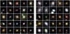 |
Fig. 1. Left: examples of strong gravitational lens systems mocked up by painting COSMOS lensed sources on PS1 stack images, and used as positive examples for training. Right: PS1 postage stamps of a subset of the 90 000 galaxies used as negative examples, including face-on spirals, massive LRGs, and field galaxies with similar gri colors as the mocks. All postage stamps are 20″ × 20″. |
4.5. Photometry of mock lens systems
Focusing the CNN lens search on a subset of the three billion sources detected in the PS1 3π survey requires a preselection of sources based on their properties released in public catalogs. For this purpose, we computed the photometry of mock lensed systems in the same way as the PS1 image processing pipeline (Magnier et al. 2020). Fixed aperture photometry is particularly important to measure reliable colors. We derived the integrated magnitudes of our mocks within the four smaller PS1 circular apertures of 1.04″ (R3), 1.76″ (R4), 3.00″ (R5), and 4.64″ (R6) radii, which are best suited to capture color gradients due to the presence of lensed arcs at angular separations of 1.5–3.0″ with respect to the lens center. The two largest of these apertures are also expected to be relatively good proxies of the integrated magnitudes of mocks. We used SExtractor in dual-image mode, with a 3σ detection threshold in r-band, and assuming an ideal sky subtraction in PS1 deep stacks (see details in Waters et al. 2020). To compute the aperture magnitudes of a given mock, the image zero-points were taken from the PS1 catalog of stack detections at the position of the LRG used to produce this mock.
The method was tested on LRG-only images by comparing SExtractor estimates with those from the PS1 catalog, for standard stacks. For the four apertures, fitting the distributions of magnitude offsets between these two estimates with Gaussian functions led to μ = 0.00–0.02 and σ = 0.02–0.05 in g band, μ = 0.00–0.01 and σ = 0.01–0.02 in r band, μ = 0.00 and σ = 0.01–0.02 in i band, which proves the overall robustness of our photometry. Unsurprisingly, the scatter only rises above these average values for the large aperture magnitudes of fainter objects, which mostly enclose background noise. These residual biases up to 0.1–0.2 mag for ≳22.0 mag likely indicate small differences in the local background subtraction between both methods, or the contamination from neighbors which were subtracted by the PS1 pipeline (Magnier et al. 2020) but not with SExtractor. Nonetheless, these offsets remain minor compared to other uncertainties in the analysis. On the contrary, Kron, Petrosian and Sersic photometry were discarded due to systematic biases with respect to values tabulated in PS1 catalogs.
5. Systematic search of strong lenses
The next sections describe the steps followed for the generic lens search on the full Pan-STARRS 3π survey.
5.1. Preselecting Pan-STARRS detections
As shown in Fig. 2, the 90 000 mock lens systems have globally bluer colors than the LRG sample due to the relative color of lensed arcs, and they are brighter than ∼70% of sources detected in the PS1 stack images. This population of fainter and bluer PS1 galaxies can be excluded from the analysis. We used simple color-magnitude cuts in the (g − i) vs. i, (g − r) vs. r, and (r − i) vs. i diagrams for the R3, R4, R5, R6 circular apertures to rule out regions in these diagrams that are not representative of the mocks (i.e., not colored in blue in Fig. 2). These cuts are conservative and include 96% of the mocks, according to the aperture magnitudes obtained in Sect. 4.5, while excluding ∼84% of PS1 sources. They were applied to the complete catalog of stack detections from PS1 DR2 using the PanSTARRS1 Catalog Archive Server Jobs System5, with detectionFlags3 > 65536 to remove multiple entries and to select detections from the optimal stack image (Flewelling et al. 2020).
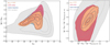 |
Fig. 2. Aperture magnitudes and colors of galaxies in the lens LRG catalog (red regions) and in the set of 90 000 mock lens systems (blue regions). The red and blue dots show the median of distributions. Left: (g − i) vs. i diagram for the R3 aperture, a circular aperture of 1.04″ radius. Right: difference in (g − i) color between the inner R3 aperture and concentric annuli between R3 and R4 (1.76″ outer radius), and between R4 and R5 (3.00″ outer radius). Gray regions mark the position of 100 000 random sources with reliable gri aperture photometry selected from the PS1 DR2 catalogs. Orange regions show galaxies with pcat > 0.5 on the catalog-level network, which match the colors and magnitudes of mocks lens systems. Solid and dashed lines show the 0.5, 1, and 2σ contours. |
The stars were removed from the resulting sample using the r-band cuts from Farrow et al. (2014):
rKron − rPSF < −0.192 + 0.120 × (rKron − 21)+0.018 × (rKron − 21)2.
This selection conservatively included 98% galaxies, those discarded being mainly at the faint end (r ≳ 21) and with higher magnitudes than our mocks. While these cuts misidentified saturated stars with r ≲ 14 as galaxies (Farrow et al. 2014), such bright sources had already been excluded from the analysis.
Regions with elevated Galactic dust extinction were removed as strong reddening could alter our selection on the catalog level. The interstellar dust reddening 2D map of Schlegel et al. (1998) were loaded with the dustmaps python interface from Green (2018). After converting to PS1 bandpasses using coefficients in Table 6 of Schlafly & Finkbeiner (2011), we applied a reddening threshold of E(g − i) < 0.3. These steps resulted in a catalog of 23.1 million galaxies for classification.
5.2. Applying machine learning to the Pan-STARRS photometry
Limitations due to download speed of PS1 cutouts from the archive can be overcome by further reducing the size of this catalog with additional selection criteria. The simple color and magnitude cuts applied to the complete PS1 catalog do not capture all photometric properties of mock lens systems, such as their precise locus on two-dimensional color-color and color-magnitude diagrams or their radial color gradients. For instance, Fig. 2 indicates that mocks are generally redder within the smaller R3 aperture of 1.04″ radius than within external, concentric annuli between R3 and R4, and between R4 and R5. These gradients are caused by the presence of bluer, lensed arcs at > 1.5″ from the lens center and disappear on the LRG-only sample. To exploit this information, we trained a simple fully-connected neural network on the photometry of mocks and random PS1 sources using aperture fluxes that ensure robust colors.
The data set contained gri fluxes in the four apertures for 90 000 lens and 90 000 nonlens examples as inputs, and the ground truth labels of 1.0 and 0.0, respectively, as outputs for binary classification. The negative examples were fluxes of random sources that matched our loose color and magnitude gri cuts in Sect. 5.1. The data set was split into training, validation, and test sets with respective fractions of 56%, 14%, and 30%. All fluxes were normalized to the average over the entire data set in order to speed up the learning process. The network architecture consisted of 12 dimensional input data, three fully connected hidden layers of 50, 30, and five neurons each, with Rectified Linear Unit (ReLU, Nair & Hinton 2010) nonlinear activations6, and a single-neuron output layer with sigmoid activation7.
During the training phase, the network derives a model for classifying galaxies in the training set as lenses or nonlenses according to their input photometry, as briefly summarized with the following stages. After the weight parameters and bias in each neuron are initialized, a subset of the training data is passed through the entire network to calculate predicted labels (forward propagation), and the difference between predictions and ground truth labels is quantified with a loss function L. This information is propagated to the network weights and biases (back propagation, Rumelhart et al. 1986) which are then modified using a gradient descent algorithm to minimize the total loss and improve the model. These stages are repeated iteratively to perform a complete pass through the entire training set, corresponding to one epoch, and then over multiple epochs until the model reaches optimal accuracy. After each epoch, the validation loss is evaluated by classifying inputs from the validation set, in order to determine whether the decrease in training loss reveals better performance or an overfitting to the training set. After training, the network performance is finally quantified using independent data from the test set. Further details can be found in the review of LeCun et al. (2015).
Network parameter optimization is performed via mini-batch stochastic gradient descent, a common variant that consists of splitting the training set into small batches and adjusting the weights according to the average corrections over each batch. Our network minimized the cross-entropy loss function which penalizes robust and incorrect predictions, and is expressed as follows for a binary classification problem
where yi are the ground truth labels, and pi the network predictions, namely scores in the range [0, 1] resulting from the sigmoid activation on the output layer. The loss was computed over each batch of size N. To avoid unbalanced splits of the data set, we used 5-fold cross-validation that consists of reshuffling the training and validation sets and building the performance metrics. Cross-validation runs trained over 500 epochs were used to optimize the neural network hyperparameters with a grid search, varying the learning rate over the range [0.0001, 0.1] and the weight decay over [0.00001, 0.01], with momentum fixed to 0.9. We trained a final network with the entire data set using an optimal learning rate and weight decay of 0.001 and 0.00001, respectively, and applying early stopping at epoch 193 that matched the lowest average loss over the cross-validation runs.
Among the 23.1 million input galaxies, 1 050 207 were assigned scores pcat > 0.5 indicating that their gri aperture photometry is consistent with the mocks. Figure 2 illustrates the network predictions by comparing the colors and magnitudes of random galaxies, mocks, and galaxies having pcat > 0.5. The good agreement between 2σ contours of mocks and pcat > 0.5 shows that the network correctly captures the position of mocks in color-magnitude diagrams, as well as their color variations within different apertures. Moreover, our photometric selection was successfully tested on the aperture fluxes of known strong lensing systems listed as grade A or B with θE = 1.0 − 3.0″ in the MasterLens database8, and with lensed arcs visible in the PS1 stack images. We therefore kept these 1 050 207 galaxies for CNN classification.
5.3. Training the convolutional neural networks
Data sets for the CNNs included 180 000 images in g, r, and i bands with the same fraction of positive (lens) and negative (nonlens) examples. Positive examples were taken from the sample of simulated lens galaxies with θE > 1.5″ described in Sect. 4.4. The choice of negative examples is strongly influencing the network predictions and was modified iteratively to improve the network performances (see Sect. 5.5). In short, we boosted the fraction of galaxies with specific morphological types using incorrect identifications of strong lenses in previous networks. This allowed the network to learn how to discriminate strongly lensed arcs from the usual contaminants such as extended arms of low redshift spirals, lenticular galaxies, and mergers, and to distinguish isolated LRGs from LRGs with the relevant strong lensing features depicted in the mocks. Our resulting set of 90 000 negative examples included:
– 30% LRGs selected directly from the catalog of SDSS LRGs on the high-end of the mass distribution used to create the mocks,
– 20% spirals classified as likely face-on galaxies in Galaxy Zoo 2 (Willett et al. 2013) and with r-band Sersic radii < 4.5″ from PS1 (Flewelling et al. 2020), to restrict to blue spiral arms with similar extension as the lensing features present in the mocks,
– 10% smooth, isolated galaxies from Galaxy Zoo 2 without bright companion and bluer colors than LRGs,
– < 1% galaxies with apparent dust lanes identified in Galaxy Zoo 2 (Willett et al. 2013),
– 32% randomly selected galaxies from the PS1 catalog, including diverse types, groups and mergers, and with negligible contamination from the rare strong lenses,
– 7% false positives from previous neural networks selected by visually classifying candidates with scores > 0.9.
Negative examples were not included in the pcat > 0.5 sample to be classified with the CNN, but they broadly followed the same color and magnitude distributions in gri bands. Some examples are shown in Fig. 1. The data set was split into training, validation, and test sets with the same proportions as before (Sect. 5.2).
We used data augmentation and applied random shifts between −5 and +5 pixels to all images so the network becomes invariant on small positional offsets. This resulted in input images of 70 × 70 pixels which conservatively included all emission from the central galaxy of interest. All survey galaxies in the set of negative examples were unique, and LRGs used multiple times in the sample of mocks were rotated by kπ/2 so they appeared only once with a given orientation in the set of positive examples. This ensured that the network was not sensitive to preferential orientations. Other common image augmentation techniques, such as image stretching, normalization and rescaling (e.g., Petrillo et al. 2017, 2019) were discarded as they did not significantly improve the learning process.
The CNN architecture was inspired from LeNet (LeCun et al. 1998) and from the lens modeling CNN of Schuldt et al. (in prep.). After the 70 × 70 × 3 input layer, it contains three convolutional layers with 11 × 11, 7 × 7, and 3 × 3 kernel sizes, and 32, 64, and 128 filters, respectively, followed by three fully connected hidden layers with 2048, 512, and 32 neurons (see Fig. 3). ReLU activations act as nonlinear transformations between each one of these layers. Max-pooling layers (Ranzato et al. 2007) with 2 × 2 kernel sizes and stride = 2 are inserted after the first two convolutional layers and are essential to make the CNN invariant to local translations of the relevant features in gri image cutouts, while reducing the network parameters. Dropout regularization (Srivastava et al. 2014) with a dropout rate of 0.5 is applied before the fully connected layers. This is an efficient regularization method that consists of randomly ignoring neurons during training in order to reduce overfitting on the training set and improve the CNN generalization. The output layer consists of a single neuron with sigmoid activation and results in a score, pCNN, in range [0, 1] which corresponds to the network lens or nonlens prediction9. Our CNN with moderate depth is well suited for binary classification of small PS1 cutouts.
 |
Fig. 3. Architecture of the convolutional neural network, inspired from LeNet (LeCun et al. 1998), and comprised of three convolutional layers with 11 × 11, 7 × 7, and 3 × 3 kernel sizes, and 32, 64, and 128 filters, respectively, followed by three fully connected hidden layers with 2048, 512, and 32 neurons. ReLU activations were applied between each layers. Max-pooling layers with 2 × 2 kernel sizes and stride = 2 were inserted after the first two convolutional layers, and dropout of 0.5 was used before the fully connected layers. |
During the training process, the CNN learns the relevant patterns in gri images by adjusting the convolutional kernel weights, through a minimization of the binary cross-entropy loss between ground truth and predicted labels. After the gradient calculation and optimization, information learned by the network is stored in the two-dimensional filters. As for the catalog-level network, we used mini-batch gradient descent with a batch size of 128 and performed five cross-validation runs. We found an optimal learning rate and weight decay of 0.0006 and 0.001, respectively, using a grid search with momentum fixed to 0.9. The number of training epochs was then chosen from the minimum average validation loss over the cross-validation runs, which corresponded to optimal network performance without overfitting.
The evolution of the training and validation loss for the network with optimized hyperparameters is shown in Fig. 4, until epoch 47 which corresponds to the lowest validation loss. The gap between both curves (generalization gap) is small, showing that the model predictions do not deteriorate much on new data with similar properties as the training set. The final network performances were characterized with the test set which was not seen during training and validation and contains about 54 000 entries. In Fig. 5, we show the model probability predictions for all lens and nonlens examples in the test set. Lenses dominate the distribution for pCNN > 0.6. The model reaches 94.2% accuracy, 93.1% purity and 95.5% completeness on this set suggesting good pattern recognition abilities on new images10. In addition, the Receiver Operating Characteristic (ROC) curve in Fig. 6 illustrates the relation between the true positive rate (TPR, the number of lenses correctly identified over the total number of lenses) and the false positive rate (FPR, the number of nonlenses identified as lenses over the total number of nonlenses) in our trained model. The curve was obtained by varying the network probability threshold for lens identification in the range [0, 1], and an ideal network would correspond to an area under curve (AUC) of 1. Our CNN gives AUC = 0.985, and can correctly identify 95.5% of lenses in the test set with a FPR of 7.1% using pCNN > 0.5, or 77.0% of lenses in the test set with a FPR of 0.8% using pCNN > 0.9. After optimizing hyperparameters and quantifying the performance of the network on the test set, we trained a final CNN with the complete data set of 180 000 labeled images and we fixed the resulting model parameters to classify the 1 050 207 galaxies with pcat > 0.5.
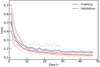 |
Fig. 4. Training of the CNN with optimized hyperparameters and using early stopping. The training loss (red curve) and validation loss (blue curve) were taken as the average of all cross-validation runs (light red and blue curves). |
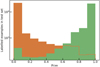 |
Fig. 5. Distribution of network predictions compared with the ground-truth for lenses (green) and nonlenses (orange) in the test set. |
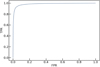 |
Fig. 6. Receiver Operating Characteristic curve for the trained CNN showing the true position rate (TPR) as function of the false positive rate (FPR) for different lens identification thresholds. The corresponding area under curve (AUC) is 0.985. |
5.4. Evaluating the network performance
The performance of the network was further evaluated on galaxies with various properties on the test set. Figure 7 depicts the normalized distributions of scores for positive examples in different bins of θE, θE/Reff, and rKron, where Reff is the effective radius from the r-band Sersic fit of the LRG-only image (Flewelling et al. 2020). Somewhat counterintuitively, scores are closer to 1.0 for lenses with θE < 2″. The low fraction of θE > 2″ in the training set might explain the slightly lower CNN performance on these systems, which generally do not have the most challenging morphologies. Histograms for θE/Reff demonstrate the ability of the network to assign pCNN closer to 1.0 for mocks with Einstein radius larger than the effective radius of the lens light distribution, where lensed arcs are in principle better deblended from the lens. We also find a higher fraction of scores pCNN > 0.9 for lens LRGs with higher rKron (i.e., fainter LRGs), perhaps because the brightest lenses outshine the lensed source emission. Nonetheless, these variations remain generally minor.
 |
Fig. 7. Normalized distributions of CNN scores for mocks lenses included as positive examples in the test set, for different ranges of Einstein radii (left), θE/Reff (middle), and rKron (right). |
Finding acceptable network performances on the test set might be misleading as it relies on our choices in simulating the strong lenses and assembling a set of negative examples. A valuable independent test consists of applying the CNN to strong lenses from the literature. For that purpose, we collected all grade A and B galaxy-scale lenses in the MasterLens catalog, restricting to Einstein radii ∼1–3″ similar to the range probed by our 90 000 mocks. These systems were discovered from various techniques including the identification of emission lines from star-forming galaxies behind LRGs using spatially-integrated spectra (SLACS, Bolton et al. 2008), and the analysis of high-quality imaging from HST (e.g., in COSMOS, Faure et al. 2008) or deep multiband surveys (e.g., CFHTLS SL2S, Cabanac et al. 2007; Gavazzi et al. 2014; More et al. 2016). Most of these lenses are not detectable in gri Pan-STARRS stacks and need to be excluded from our test set. We thoroughly scanned all PS1 gri single-band and 3-color images of this sample to find those with detected lensed arcs, and assembled a test set of 16 systems. While these published lenses have colors, zd, zs, and configurations similar to our mocks, some of their multiple images are strongly blended with the lenses and difficult to identify with PS1 data.
Pan-STARRS cutouts of these 16 lenses were scored with our trained neural network and the results are presented in Fig. 8. A total of 14/16 lenses are correctly identified as pCNN > 0.5 by the CNN, while 9/16 and 7/16 have higher scores pCNN > 0.8 and pCNN > 0.9, respectively. SL2SJ0217−0513 and SDSSJ1112+0826 are the two incorrect classifications. SL2SJ0217−0513 has a faint lens galaxy falling in the upper range of the redshift distribution (zd = 0.646) and blended with a faint blue arclet. It is worth noting that the network performs better for SDSSJ1110+3649 (pCNN = 0.971) which has a similar morphology to SL2SJ0217−0513, but with the addition of a low S/N, blue counter image on the other side of the lens galaxy. SDSSJ1112+0826 has typical properties of our mocks but lacks a bright counter image. On the other hand, lenses with well-detected and deblended arcs and counter images (e.g., SDSSJ1430+4105, SDSSJ0201+3228, CSWA21) have high scores, showing that the network is able to extract relevant features.
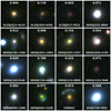 |
Fig. 8. Three-color images of the 16 confirmed lens systems in the MasterLens database that have clear strong lensing signatures in Pan-STARRS images, and Einstein radii of 1–3″ similar to our mocks. The CNN scores are displayed at the top of each panel. Images are 15″ × 15″. |
Our comparison extends to systems with Einstein radii below the 1.5″ cutoff applied to our simulations. The CNN performance in this regime remains acceptable, as illustrated by the scores of 0.786, 0.612, and 0.971 assigned respectively to SDSSJ1134+6027, SDSSJ2156+1204, SDSSJ2231−0849 that have θE ∼ 1.1″. In contrast, with θE = 3.26″ due to its group-scale environment (Auger et al. 2013), CSWA21 falls on the upper range of the Einstein radius distribution that is underrepresented with only a few hundred examples in our training set. This system is nonetheless given a score of 0.873 and confirms that the CNN can identify these simple configurations. Interestingly, the four systems with ≥4 magnified images according to the MasterLens database have pCNN > 0.9. The small number of test lenses however prevents robust estimates of the method purity and completeness.
5.5. Discussion on the CNN training
The final version of the CNN from Sect. 5.3 was selected from a range of networks with different architectures, after testing the impact of the training set content. To identify the optimal network, we compared scores assigned to the 16 known test lenses and required low false positive rates by examining gri cutouts of the few hundred galaxies with highest scores pCNN. Overall, different choices of positive and negative examples had much stronger impact, inducing variations in the number of good lens candidates from visual inspection by a factor of ≳10 due to the network learning different features, while changes in the CNN architecture only offered slight improvements.
The sets of negative examples tested include: (1) random PS1 sources drawn from the preselection in Sect. 5.1; (2) typical LRGs selected as in Eisenstein et al. (2001), mostly less massive than LRGs in mocks; (3) high-mass LRGs similar to those used in Sect. 4; (4) a combination of LRGs, face-on spirals, and random sources (varying the fractions of LRGs and contaminants). Scores on the MasterLens systems from CNNs using sets (1) and (4) were comparable to those in Fig. 8, but introduced an overwhelming number of ≳400 000 galaxies with pCNN > 0.5 and ≳250 000 with pCNN > 0.9 implying high false positive rates, and were ruled out. Other sets of positive examples were tested by (1) modifying the θE lower limit, and (2) suppressing the artificial boost in arc brightness to get more realistic lens over source flux ratios. Both CNNs trained on fainter arcs, more strongly blended with the lens significantly reduced the fraction of genuine lens examples with scores pCNN ∼ 1 and were also discarded.
Our tests on the architecture include: (1) adding and removing one convolutional layer, or one fully-connected layer; (2) changing the number of neurons, the kernel sizes or number of feature maps in these layers; (3) using smaller or larger strides on the max-pooling layers; (4) modifying the dropout rates; (5) implementing batch normalization (Ioffe & Szegedy 2015). Each of these changes degraded the network performance as measured from the loss and ROC curves on the test set, and from the 16 MasterLens systems. Using dropout normalization before fully connected layers (as in Fig. 3) turned out to be the most efficient solution to reduce overfitting.
5.6. Visual classification
Galaxies with high CNN scores, pCNN, were visually inspected by different authors to assign a final grade. We started classifying galaxies with pCNN close to 1.0, and progressively lowered the threshold to introduce additional galaxies until the fraction of reliable candidates from visual inspection became too low.
We graded the single-band and 3-color PS1 cutouts in gri bands, zoomed to 12″ × 12″, and optimally displayed with linear and arcsinh scaling using dedicated scripts to emphasize faint, sometimes blended strong lensing features11. To aid the visual classification, we plotted grz single-band and 3-color postage stamps from the DESI Legacy Imaging Surveys that significantly overlaps the PS1 3π survey footprint on the extragalactic Northern sky, and that provides slightly deeper, higher quality images (Dey et al. 2019), and we plotted residual frames from subtraction of the best-fit light profile. On smaller regions of the sky, we also included gri images from HSC DR2 wide-field surveys (Aihara et al. 2019). The set of CNN candidates was divided into four equal parts, each inspected either by R. C., S. S., S. H. S., or S. T., in order to assign one of the following grades: 0: nonlens, 1: maybe a lens, 2: probable lens, 3: definite lens, similarly to Sonnenfeld et al. (2018) and Jacobs et al. (2019a). All candidates with grades ≥2 from this first iteration were then inspected by the three other authors, so final grades were averaged over the four authors. The output list of candidates corresponds to average grades ≥2.
Nonlenses are galaxies clearly identified as nearby spirals, ring galaxies, groups, or other contaminants from their morphology, or cutouts with artifacts. Candidates listed as grade 1 have faint companions or weakly distorted features suggesting possible strong lensing signatures, but may also correspond to galaxy satellites or spiral arms. Probable lenses show multiple elongated sources with similar colors, and orientation and angular separation expected for counter-images, while the available 3-color images cannot firmly rule out contaminants. Those assigned grades of 3 have similar, although brighter, nonblended and unambiguous signatures of galaxy-scale strong lenses.
6. Results and discussion
6.1. Final candidates from visual inspection
Out of the 1.1 million galaxies the CNN scores 598 130 with pCNN = 0, and 105 760, 12 382, and 1714 as candidate lenses with pCNN > 0.5, pCNN > 0.9, and pCNN = 1, respectively. Scores pCNN > 0.5 amount to 10% of sources ranked by the CNN, and only 0.5% of the input catalog of 23.1 million galaxies. The human inspection process is necessary to increase purity of the candidate sample. However, a systematic visual classification of galaxies with pCNN > 0.5 would be unrealistic and we use a higher pCNN threshold which impacts the purity and completeness in a way that is difficult to quantify. Predictions for mock lenses on the test set (see Fig. 5) and for known lenses (see Fig. 8) suggest that the majority of good candidates have scores pCNN > 0.9 with only a few more in the range 0.5 < pCNN < 0.9, and we therefore started inspecting all 12 382 with pCNN > 0.9. As the fraction of visual grades ≥2 quickly drops with decreasing CNN scores, down to ≲1% when extending to 0.8 < pCNN < 0.9, we restricted our final classification to pCNN > 0.9.
Our selection results in 321 high-confidence candidates with grades ≥2 (hereafter, grades refer to the average grades from the visual inspectors). Respective fractions of 36%, 34%, and 30% of these candidates have scores in the intervals 0.99 < pCNN ≤ 1.00, 0.95 < pCNN ≤ 0.99 and 0.90 < pCNN ≤ 0.95, which demonstrates that the CNN learns meaningful information and assigns high scores for most of the probable or definite lenses. The rate of grades ≥2 over the 12 382 galaxies with pCNN > 0.9 is about 2.5%. This fraction is slightly lower but comparable to previous CNN lens searches using deeper, higher quality imaging surveys (KiDS DR4, DES Year 3, Petrillo et al. 2019; Jacobs et al. 2019a). This is not surprising as some of these searches have focused on catalogs of LRGs with robust photometry and are less subject to contamination by low-redshift spirals. Obtaining equivalent performance suggests that our initial catalog-level classification plays an important role in our systematic search that balances the suboptimal imaging quality of the PS1 3π survey. Finally, 37 additional candidates from previous CNNs with pCNN = 1.0 and grades ≥2 are included (see Sect. 5.5), bringing the total number of resulting lens candidates to 358 from our two-step search.
Examples of good candidates and false positives (grades ≤1) after visual inspection are shown in Fig. 9. In most cases, false positives belong to specific galaxy types frequently misclassified by the network such as nearly face-on spirals with obvious and extended arms, nearby lenticular galaxies, and bright LRGs with faint unlensed companions. Galaxy groups, mergers with perturbed morphologies, and cutouts with background artifacts are more rare. Other ambiguous systems listed as false positives are galaxies with red bulges and faint arms, with color gradients or companions, where all components are blended and mimic lensed arcs.
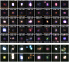 |
Fig. 9. Top: Pan-STARRS 3-color gri images of a subset of candidates with grades ≥2 from visual inspection of CNN scores pCNN > 0.9 (the complete figure is available in Appendix A). Numbers displayed on top of each panel are CNN scores (pCNN, left) and average visual grades (right). Candidates with PS1 names marked in orange have been previously published in the literature (see Table 1 and Sect. 6.1) Those marked in blue show unambiguous spectral signatures of high-redshift background sources in our inspection of SDSS BOSS DR16 data. Bottom: examples of random false positives with pCNN = 1. All cutouts are 15″ × 15″. |
The PS1 lens candidates were cross-matched with galaxy-scale strong lenses from previous searches with the status of spectroscopally confirmed or candidate systems, by building upon and expanding the current MasterLens database. We compiled grade A and B systems (or equivalent) from a number of recent searches based on optical and near-infrared imaging from DES (Diehl et al. 2017; Jacobs et al. 2019b,a), CFHTLS (More et al. 2016; Jacobs et al. 2017), KiDS (Petrillo et al. 2017, 2019; Li et al. 2020), DESI (Huang et al. 2020a), and HSC (Wong et al. 2018; Sonnenfeld et al. 2018, 2020; Jaelani et al. 2020). Since our network may also be sensitive to lensed quasars with colors and configurations similar to our mock lenses, we also cross-matched with the all-sky database of ∼220 confirmed lensed quasars in the literature (Lemon et al. 2019, and references therein)12, and with previously identified lensed quasars from HSC (Chan et al. 2020) and from PS1 (Rusu et al. 2019). For the candidates not included in those tables, we searched in the SIMBAD Astronomical Database13.
To our knowledge, besides the test lenses from the MasterLens database, 23 of our 358 CNN candidates are already listed in the literature and corresponding references are listed in Table 114. The vast majority of them are also galaxy-scale strong lens candidates from ground-based multiband imaging searches and lack both spectroscopic and high-resolution imaging follow-up. The only galaxy-galaxy lens systems confirmed with spectroscopy or space-based imaging are PS1J0143+1607, PS1J0145−0455, PS1J2343−0030, and PS1J0454−0308. Firstly, PS1J0143+1607 is CSWA 116, discovered through the search of blue lensed features near LRGs in SDSS imaging (Stark et al. 2013). Its properties (zd = 0.415, zs = 1.499, θE = 2.7″) are very similar to our mock lenses, and the system was assigned pCNN = 1.0 and a visual grade of 2.75. Secondly, PS1J0145−0455 is CSWA 103, also presented by Stark et al. (2013), and has zd = 0.633, zs = 1.958, and θE = 1.9″, akin to our mocks. It has pCNN = 1.0 and a visual grade of 2.50. Thirdly, PS1J2343−0030 is a SLACS lens with zd = 0.181 and zs = 0.463 which was discovered and modeled by Auger et al. (2009) using SDSS spectroscopy and HST imaging. It has an Einstein radius of 1.5″, higher than the majority of lenses in the SLACS sample, which explains its elevated scores from the CNN (pCNN = 0.917) and PS1 cutout inspection (2.50). Lastly, PS1J0454−0308 (pCNN = 1.000 and grade = 2.75) is a peculiar system thoroughly studied in Schirmer et al. (2010), where the main lens is the brightest elliptical galaxy of a fossil group at z = 0.26 only 8′ from the MS0451−0305 cluster at z = 0.54. The HST F814W frame clearly resolves the background source into an extended arc and a compact counter image, corresponding to θE = 2.4″. Most other galaxy-galaxy lenses in the literature were missed by our selection due to limited PS1 depth or lens configurations not represented in our mocks (e.g., higher Einstein radii). Finally, two of these 23 published systems are confirmed lensed quasars. PS1J2350+3654 (pCNN = 1.0 and grade of 2.25) was discovered in Gaia DR2 (Lemon et al. 2019), and PS1J1640+1932 (pCNN = 1.0 and grade of 2.25) from SDSS (Wang et al. 2017).
Final list of galaxy-scale strong lens candidates with lens LRGs from our systematic search in Pan-STARRS.
Postage stamps of the 335 newly-discovered and 23 published galaxy-scale lens candidates from our Pan-STARRS CNN search are shown in Fig. 9 and in Appendix A, together with pCNN and visual inspection grades. Given that some visual identifications rely on Legacy imaging, which is sometimes deeper than PS1, we also show Legacy 3-color images of our candidates located in the Legacy footprint in Appendix A.
6.2. Ancillary spectroscopy
We inspected SDSS BOSS spectra from the 16th data release available for 104 out of 358 lens candidates, in order to characterize the candidate lens galaxies and to search for spectral signatures of high-redshift background galaxies. This approach was previously used to select the SLACS sample (Bolton et al. 2008) and relies on spectral features captured within the small, 2″ diameter aperture fibers. Firstly, our examination results in 84 spectra of typical LRGs at intermediate redshift with bright continuum, prominent 4000 Å break, deep stellar absorption lines, and non- or very faint [OII]λλ3727 detections indicating evolved stellar populations with little residual star formation. Secondly, we obtain seven LRG-like spectra with two or more emission or absorption lines falling at a different and concordant redshift, higher than the LRG redshift, and indicating the presence of a background galaxy. Two of them are already published as confirmed strong lens systems: PS1J2343−0030 as part of the SLACS sample (Auger et al. 2009), and PS1J1640+1932 (lensed quasar from Wang et al. 2017). Thirdly, we find eight LRG-like spectra overlaid with a single bright, high-redshift emission line consistent with [OII]λλ3727 from a background star-forming galaxy at 0.95 < z < 1.50. Although the line widths and resolved double-peaked profiles are those expected for the [OII] doublet, other bright emission lines (Hβλ4863, [OIII]λ4960 and [OIII]λ5008) are redshifted out of the BOSS spectral window and we consider these identifications as ambiguous. Lastly, three cases show clear signatures of star-forming galaxies at z < 0.3, which likely have blue arms misidentified as lensed arcs, one QSO at z = 0.5890, and one star. These five systems are considered as false positives.
Finding a vast majority of LRGs15 and only 3/104 star-forming galaxies at lower redshift demonstrates the validity of our method. This result shows that our CNN and visual inspection method predominantly selects the targeted population of galaxy-scale strong lens candidates with lens LRGs, and efficiently distinguishes strong lensing features from usual interlopers (e.g., spiral arms, tidal features, blue rings). Moreover, the five false positives (PS1J2249+3228, PS1J1551+2156, PS1J1452+1047, PS1J0834+1443, and the QSO PS1J1156+5032) are all listed as lower confidence candidates with grades ≤2.25.
The rarity of spectroscopic signatures from lensed galaxies is not surprising because the 2″ BOSS fibers enclose little lensed source emission in the θE ≳ 1.5″ systems targeted by our search. Background line flux can only be detected in few favorable cases, like in the presence of counter-images closer to the lens center. In addition, emission lines in most lensed galaxies might be too faint for SDSS spectroscopy, and the observable spectral band of BOSS excludes Hβ4863, [OIII]4960 and [OIII]5008 for z > 0.9, which rules out multiple line detections for the majority of sources expected at z > 1.
The only Pan-STARRS candidate robustly confirmed as a strong lens system is PS1J1415+1112. Pan-STARRS imaging spatially resolves the system into a quadruply-imaged background source forming a typical fold configuration, and with redder color than the lens LRG (Fig. 9). The best-fit model from the BOSS pipeline primarily identifies spectral features from the foreground LRG at zd = 0.3155, but poorly fits the continuum and remarkably prominent Balmer absorption lines at λobs > 8000 Å (Fig. 10). These features are associated with the background galaxy at zs = 1.185. Further inspection of the BOSS spectrum shows that the strong Balmer absorption lines, together with the weak 4000 Å break indicative of relatively young stellar populations, and the lack of nebular emission lines at zs = 1.185 suggesting little on-going star formation, favor the scenario of a recently quenched galaxy. To verify this hypothesis, we used the BC03 stellar population synthesis models (Bruzual & Charlot 2003) to combine the SED template of an elliptical galaxy at zd = 0.3155 with 7 Gyr old stellar populations and solar metallicity with various templates of post-starbursts at zs = 1.185. After varying the stellar age, metallicity, and dust attenuation, we found that rescaling the SED of a young galaxy with 25 Myr old stellar populations, no on-going star formation, and Z = 0.2 Z⊙ correctly fits the overall wavelength range in Fig. 10. Together with the red colors of multiple images this adds further evidence that the lensed galaxy has indeed ceased star formation recently.
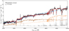 |
Fig. 10. Pan-STARRS lens candidate with prominent Balmer absorption features from a background galaxy at zs = 1.185 blended with the BOSS spectrum of the lens LRG at zd = 0.3155. The black and gray lines show the spectrum observed with a fiber of 2″ diameter and the 1σ noise level, respectively, and the blue line corresponds to the best-fit LRG template from the automated SDSS pipeline at λ < 8000 Å (see inset), which poorly fits the continuum and Balmer lines at longer wavelengths. The red line shows that combining the SED templates of an LRG at zd = 0.3155 (brown curve) and a recently quenched galaxy at zs = 1.185 (orange curve) correctly fits the spectrum over the entire range (see details in text). |
The last four CNN candidates showing multiple emission lines from a background, possibly lensed galaxy do not exhibit such clear configurations in Pan-STARRS and Legacy gri images. Their BOSS spectra reveal simultaneous detections of [OII]λλ3727, Hβλ4863, [OIII]λ4960, and [OIII]λ5008 on top of the prominent stellar continuum from the foreground LRG (see Fig. 11). The first three are PS1J2345−0209 with zLRG = 0.2940 and zs = 0.6581, PS1J1134+1712 with zLRG = 0.3752 and zs = 0.8121, and PS1J0917+3109 with zLRG = 0.2386 and zs = 0.8198. These candidates were listed as probable lenses from our grades and, although zLRG, zs, and  suggest plausible Einstein radii ∼1″ for singular isothermal sphere profiles, high-resolution follow-up imaging is needed to ascertain their configuration. These data will determine whether the background, spectroscopically-confirmed galaxies are those visually identified with Pan-STARRS and indeed multiply-imaged, or whether they are out of the strong lensing regime. Lastly, PS1J1724+3146 comprises a foreground LRG at zLRG = 0.2097 and a background source at zs = 0.3461, likely too close to the lens to enter the strong lensing regime.
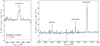 |
Fig. 11. Example of a lens candidate with multiple emission lines from a high-redshift background galaxy overlaid on the SDSS BOSS spectrum of the foreground LRG. The black, gray and blue lines show the observed spectrum, the 1σ noise level, and the best-fit SDSS template for the LRG, respectively. The spectrum is zoomed on the spectral features associated with the background line-emitter at z = 0.8198 rather than with the LRG at z = 0.2386. |
6.3. Properties of candidates
Our visual inspection stage implies that resulting lens candidates have morphologies and configurations easily detectable by the human eye. Figure 9 confirms that higher grades are given to systems with extended arcs, clear counter images and often compact lens light profiles. Postage stamps make it clear that our most reliable systems have relatively brighter and distorted arcs (as plausible strongly lensed background galaxies) in gri bands which will facilitate their future follow-up. Interestingly, besides the numerous blue arcs (e.g., PS1J1647+1117, PS1J1508−1652), several candidates have lensed sources redder than the foreground LRGs (e.g., PS1J1559−3147, PS1J1445+3649) and others have compact, nearly point-like morphologies suggestive of lensed quasars (e.g., PS1J1926−2138). Since the presence of possible counter images is a prerequisite for lens identifications, our candidate set is presumably biased toward higher fractions of quads than doubles, at least for grades ∼3. Other biases on the relative positions of lenses and sources might also arise. For instance, although our tests suggest that systems with θE/Reff < 1 are correctly classified by the CNN, with only minor differences in pCNN with respect to θE/Reff > 1 (Fig. 7), candidates and known lenses recovered by visual inspection should be relatively less blended and lie on the high-end of the θE/Reff distribution. Quantifying this effect is nevertheless an arduous task due to uncertainties in reliably measuring Reff from Pan-STARRS imaging. As previously mentioned, systems with θE differing from simulated lenses in our training set are likely all discarded.
Our 358 candidates have lens redshifts in the range zd ∼ 0.15 − 0.65. The distribution does not change much between candidates with confirmed lens zspec from SDSS, and those with more uncertain SDSS zphot due to lens and source blending. It closely matches the lens redshift ranges in other samples selected through multiband, ground-based imaging such as CASSOWARY (Stark et al. 2013) and SL2S (Sonnenfeld et al. 2013). Interestingly, Pan-STARRS candidates with SDSS stellar velocity dispersion have  km s−1. This is significantly lower than
  km s−1 in the set of LRGs for simulations (Sect. 4.4), indicating that lens LRGs in our candidate set are less massive on average.
To understand implications of such differences in σ* we followed Petrillo et al. (2017) and, for each lens candidate with zd and σ* available from BOSS, we calculated Einstein radii for a singular isothermal sphere profile and different source redshifts spanning the most plausible zs = 0.5 − 3.0 range. We assumed σSIS ∼ σ*. In the vast majority of cases (86%), Einstein radii predicted from the lens galaxy dynamics match the approximate θE ∼ 1 − 2″ of PS1 candidates from a basic inspection of 3-color images in Fig. 9. This range is also expected from construction of the training set and our CNN selection function. Predicted and observed image configurations usually match for zs > 1. This qualitative test argues in favor of plausible lens configurations and few contaminants despite the moderate σ* from BOSS.
In some cases, the large Einstein radii ≳1.5″ are likely to be partly attributed to a contribution from the environment of the primary lens galaxy, probably from a smooth dark-matter halo associated with an extended group- or cluster-scale structure (Oguri 2006). As a matter of fact, obtaining a few strong lens candidates with θE in the same range as our lens simulations but with lower SDSS stellar velocity dispersions proves that, if they are genuine strong lenses, they host moderately massive lens LRGs with significant external shear and magnification contributions from the environment. We verified that some of our Pan-STARRS candidates are indeed matching the position of the central brightest cluster galaxy of SDSS clusters (e.g., PS1J0907+4233, PS1J2153+1154, PS1J1417+2120, PS1J1210+2843, PS1J1730+3405, Szabo et al. 2011), and of candidate galaxy clusters from a red sequence search in DES imaging (e.g., PS1J0919+0336, PS1J2233+3012, PS1J1210+2843, PS1J1414+6447, Rykoff et al. 2016). This environmental effect is well illustrated by the case of PS1J0454−0308 characterized in Schirmer et al. (2010). We also found that PS1J2210+0620 and its bright red arc of ∼8″ extension lie behind the core of Abell 2422 galaxy cluster (Abell et al. 1989). Lastly, PS1J1142+5830 is located in the field of the rich, X-ray luminous galaxy cluster MACSJ1142.4+5831 at z = 0.325, also known as Abell 1351, which has a bimodal velocity distribution suggesting an on-going merger (Barrena et al. 2014). The SDSS photo-z of PS1J1142+5830 is consistent with the cluster redshift but our candidate is offset by 1.3′ from the brightest cluster galaxy.
The Pan-STARRS gri photometry of our 358 candidates is comparable to that of our lens simulations. Observed (g − i) colors of the deflector central regions within 2″ diameter apertures range between 1.3 and 2.7 mag and broadly follow the color distribution of mocks and pcat > 0.5 galaxies in Fig. 2. Our best candidates are therefore representative of the global sample and visual inspection does not introduce significant biases in terms of lens color. Kron (g − i) colors from blended deflector and source emissions are ∼0.3 mag lower because lensed arcs are predominantly bluer than the lens LRGs. Given uncertainties on the lensed source colors, quantitative analyses would require subtracting the lens LRG light profile, a hazardous task with Pan-STARRS imaging. However, it is worth noting that a majority of pCNN > 0.9 systems with blue arcs closely mimicking extended arms of star-forming spirals were conservatively discarded by visual inspection, while systems with similar configurations but redder arcs where considered less ambiguous and assigned higher grades. Consequently, the output set is likely biased toward a higher fraction of red lensed arcs compared to all genuine lens systems assigned pCNN > 0.9.
We did not find significant correlations between average grades and photometric properties. Although our high and lower-confidence candidates have comparable lens brightness, those with higher grades have slightly redder lenses by ∼0.15 mag in (g − i) on average. Mean lens redshifts and velocity dispersions are also increasing in the top half of the candidate set, by 0.05 and 50 km s−1, respectively.
6.4. Discussion
Our study demonstrates that a two-step approach combining catalog-level and image-level classifications, as already applied to lensed quasars searches (Agnello et al. 2015), is efficient in selecting galaxy-scale strong lenses from very wide-field surveys without imposing restrictive cuts on the input galaxy catalog. Using three bands and multiaperture photometry, our catalog-level neural network conveniently reduces the sample size for CNN classification to the order of one million sources which, in the case of Pan-STARRS, allows us to download all gri cutouts within a manageable amount of time of about one week. This first stage will be particularly beneficial to overcome data volume limitations in the new era of deep, large scale surveys such as LSST. At the same time, the low false negative rate and good performance on known lens systems of our catalog-level network applied to Pan-STARRS photometry shows that this stage discards very few potentially interesting systems. After that, we obtain encouraging results from our CNN combined with visual inspection. The compilation of 330 newly-discovered lens candidates (after removing the five false-positives identified from SDSS BOSS spectra) and confirmation of 23 lenses already selected from other, more suitable surveys (e.g., DES, KiDS) demonstrates the efficiency of our approach regardless of the limited depth and seeing in Pan-STARRS.
The strategy presented in this paper is expected to be easily applicable to the deeper LSST gri stacks in order to identify the large set of new, wide-separation galaxy-scale lenses from this survey. The simulations of Collett (2015) suggest that the LSST final stacks in gri bands will yield about 39 000 detectable lens systems, with θE greater than the seeing FWHM and large enough to spatially-resolve multiple images, and with total S/N of lensed arcs > 20 in at least one band. Under these assumptions, future LSST lenses will mainly cover θE = 1 − 3″, a similar range as our Pan-STARRS candidates, and their systematic identification will be crucial for several science cases including the search for strongly lensed SNe with spatially-resolved multiple images for early-phase SN spectroscopy and cosmography (Suyu et al. 2020). In order to achieve this, we can customize our simulation pipeline of realistic Pan-STARRS mock lenses to produce LSST mocks and quickly assemble a training set, by using gri cutouts of the relevant LRG lenses from LSST stacks rather than Pan-STARRS. Extending the search to broader populations of lens galaxies might also become feasible, in light of the ∼4 mag deeper gri LSST stacks.
Tests on the CNN performance presented in this paper are likely valid essentially for Pan-STARRS seeing and depth, while better imaging quality should enable identifications of broader, more complex image patterns and would likely benefit from updates on the neural network. The main challenge is the minimization of false positives which, given the rarity of strong lenses per deg2, will largely dominate the sample of CNN candidates even with FPR down to 1% or less. Potential avenues for improvements include adding other convolutional layers or boosting the learning process with residual networks (He et al. 2016), as the latter might give better performance for image features not represented in the training data (for LSST simulations, see Lanusse et al. 2018). A possibility would be to use CNNs optimized for image outlier detection (e.g., Margalef-Bentabol et al. 2020), either to identify strong lenses as the outlier class, or simply to exclude cutouts with partial coverage, background artifacts or other anomalies before classification. In addition, although Teimoorinia et al. (2020) found little difference with single-band HST images, implementing additional classes for the usual interlopers (spirals, ring galaxies, ...) might help distinguish signatures of strong lenses in gri bands. Our Pan-STARRS lens search demonstrates that ultimately, most progress should come from the choice of positive and negative examples in the training set (see Sect. 5.5). Highly-realistic lens simulations are one of the main ingredients (see Lanusse et al. 2018). For instance, as multiple images are strongly blended with lenses in about half of the mocks produced in Sect. 4.4, one could only include those visually classified as definite lenses from their bright arcs and unambiguous configurations. Fine-tuning the selection of positive examples in this way could help the network assign high scores exclusively to robust candidates that are worth including for follow-up campaigns.
Reducing the false positive rates and making sure that only high-confidence candidates get pCNN ∼ 1 will be crucial for future lens searches in the LSST era. However, the most efficient neural networks should provide orders of magnitudes more lens candidates than Pan-STARRS and their systematic visual inspection might become unrealistic. Assembling complete strong lens samples will therefore require one to abandon this nonautomated, human-classification stage and to search for alternatives. For instance, calibrating the CNN scores as probabilities (e.g., Guo et al. 2017) could help quantify purity and completeness, and automatically select a subset of candidates for high-resolution imaging or spectroscopic follow-up.
7. Conclusion
In this paper, we presented a systematic search for wide-separation, galaxy-scale strong lenses in Pan-STARRS using machine learning classification of gri images from the 3π survey on the entire Northern sky. We focused our search on massive LRGs acting as strong lenses and producing Einstein radii ≥1.5″, and we simulated a set of highly-realistic mocks by painting lensed arcs on Pan-STARRS image cutouts of LRGs with known redshift and velocity dispersion from SDSS. This strategy ensures that mocks include background artifacts and field galaxies, and that the network becomes invariant under the small scale exposure and FWHM variations on the survey stacks.
We computed the gri aperture photometry of mocks to preselect a conservative catalog of 23.1 million sources, and followed a two-step approach for classification: (1) a catalog-based neural network on the source photometry, (2) a CNN trained on gri image cutouts. The catalog-level network assigned pcat > 0.5 for 1 050 207 galaxies while excluding little known lenses from the MasterLens catalog. The image-level network then yielded sets of 105 760 and 12 382 candidates with scores pCNN > 0.5 and > 0.9, respectively. We visually inspected those with pCNN > 0.9 and combined with previous CNNs to assemble a final set of 330 high-quality newly-discovered candidates with average visual grades ≥2. Publicly available BOSS spectroscopy of the lens candidates’ central regions proves that the vast majority are indeed LRGs at z ∼ 0.1 − 0.7, and five newly-discovered candidates show robust signatures of blended, high-redshift background sources. Pan-STARRS clearly resolves one of them as a quadruply-imaged red galaxy at zs = 1.185 (likely recently quenched), behind a lens LRG at zd = 0.3155.
This new set of bright lens candidates is particularly valuable for future lensed SNe searches. Strong lenses with such image separations are indeed likely to produce long time delays of a few days to weeks which alleviates difficulties affecting θE < 1″ lensed SNe such as iPTF16geu and allows one to measure accurate, microlensing-free time delays for cosmography. Such time delays are also well-suited to trigger timely imaging and spectroscopic follow-up of a SN reappearance to characterize the SN’s early-phase behavior within a few days after explosion. In the meantime, validating these Pan-STARRS lens candidates and deriving strong lensing models will require high-resolution imaging and spectroscopic follow-up.
Our CNN exhibits good performance on known lenses detected in Pan-STARRS, correctly classifying 14/16 systems as lenses and assigning scores pCNN > 0.9 to 7/16. We found that CNN predictions strongly depend on the construction of the training set but little on the network architecture. Our search also recovered 23 confirmed or candidate strong lenses in the literature out of the MasterLens catalog. In the near future, the release of deep stacks with best seeing conditions in smaller fields as part of Pan-STARRS DR3 will give the opportunity to extend our search to optimal PS1 data quality. In addition, we expect that the efficient and automated two-step classification method presented in this paper will be applicable to the deep gri image stacks from LSST with only minor adjustments.
Galaxy Zoo: CANDELS (Simmons et al. 2017) performs similar classifications using deeper, multiband HST images but only over a subset of the COSMOS field (Grogin et al. 2011; Koekemoer et al. 2011) and strongly restricts the sample size.
Code adapted from https://github.com/esavary/Visualisation-tool
In addition, some systems have also been found independently and concurrently in DESI Legacy Surveys DR8 by Huang et al. (2020b): PS1J0717+4624, PS1J0324−1020, PS1J1749+2330, and PS1J1903+5225 are assigned A or B grades and 16 other candidates are assigned C grades by Huang et al. (2020b).
Acknowledgments
We would like to thank the anonymous referee for thoroughly reading the manuscript and providing useful suggestions. We wish to thank Matt Auger and Alessandro Sonnenfeld for sharing python scripts for spectrum visualization. We also thank B. Clément, F. Courbin, S. Huber, C.-H. Lee, D. Sluse and A. Yıldırım for useful discussions and feedback about this work. RC, SS and SHS thank the Max Planck Society for support through the Max Planck Research Group for SHS. This project has received funding from the European Research Council (ERC) under the European Union’s Horizon 2020 research and innovation program (LENSNOVA: grant agreement No 771776). This works has also been in part supported by the Swiss National Science Foundation (SNSF) and by the European Research Council (ERC) under the European Union’s Horizon 2020 research and innovation program (COSMICLENS: grant agreement No 787886). The Pan-STARRS1 Surveys (PS1) and the PS1 public science archive have been made possible through contributions by the Institute for Astronomy, the University of Hawaii, the Pan-STARRS Project Office, the Max-Planck Society and its participating institutes, the Max Planck Institute for Astronomy, Heidelberg and the Max Planck Institute for Extraterrestrial Physics, Garching, The Johns Hopkins University, Durham University, the University of Edinburgh, the Queen’s University Belfast, the Harvard-Smithsonian Center for Astrophysics, the Las Cumbres Observatory Global Telescope Network Incorporated, the National Central University of Taiwan, the Space Telescope Science Institute, the National Aeronautics and Space Administration under Grant No. NNX08AR22G issued through the Planetary Science Division of the NASA Science Mission Directorate, the National Science Foundation Grant No. AST-1238877, the University of Maryland, Eotvos Lorand University (ELTE), the Los Alamos National Laboratory, and the Gordon and Betty Moore Foundation. Based in part on data collected at the Subaru Telescope and retrieved from the HSC data archive system, which is operated by Subaru Telescope and Astronomy Data Center at National Astronomical Observatory of Japan. The Hyper Suprime-Cam (HSC) collaboration includes the astronomical communities of Japan and Taiwan, and Princeton University. The HSC instrumentation and software were developed by the National Astronomical Observatory of Japan (NAOJ), the Kavli Institute for the Physics and Mathematics of the Universe (Kavli IPMU), the University of Tokyo, the High Energy Accelerator Research Organization (KEK), the Academia Sinica Institute for Astronomy and Astrophysics in Taiwan (ASIAA), and Princeton University. Funding was contributed by the FIRST program from Japanese Cabinet Office, the Ministry of Education, Culture, Sports, Science and Technology (MEXT), the Japan Society for the Promotion of Science (JSPS), Japan Science and Technology Agency (JST), the Toray Science Foundation, NAOJ, Kavli IPMU, KEK, ASIAA, and Princeton University. This paper makes use of software developed for the Rubin Observatory Legacy Survey of Space and Time. We thank the LSST Project for making their code available as free software at http://dm.lsst.org
References
- Abell, G. O., Corwin, H. G., Jr., & Olowin, R. P. 1989, ApJS, 70, 1 [NASA ADS] [CrossRef] [EDP Sciences] [Google Scholar]
- Agnello, A., Kelly, B. C., Treu, T., & Marshall, P. J. 2015, MNRAS, 448, 1446 [NASA ADS] [CrossRef] [Google Scholar]
- Aihara, H., Armstrong, R., Bickerton, S., et al. 2018, PASJ, 70, S8 [NASA ADS] [Google Scholar]
- Aihara, H., AlSayyad, Y., Ando, M., et al. 2019, PASJ, 71, 114 [CrossRef] [Google Scholar]
- Auger, M. W., Treu, T., Bolton, A. S., et al. 2009, ApJ, 705, 1099 [NASA ADS] [CrossRef] [Google Scholar]
- Auger, M. W., Budzynski, J. M., Belokurov, V., Koposov, S. E., & McCarthy, I. G. 2013, MNRAS, 436, 503 [NASA ADS] [CrossRef] [Google Scholar]
- Avestruz, C., Li, N., Zhu, H., et al. 2019, ApJ, 877, 58 [CrossRef] [Google Scholar]
- Barnabè, M., Czoske, O., Koopmans, L. V. E., Treu, T., & Bolton, A. S. 2011, MNRAS, 415, 2215 [NASA ADS] [CrossRef] [Google Scholar]
- Barnabè, M., Spiniello, C., Koopmans, L. V. E., et al. 2013, MNRAS, 436, 253 [NASA ADS] [CrossRef] [Google Scholar]
- Barrena, R., Girardi, M., Boschin, W., De Grandi, S., & Rossetti, M. 2014, MNRAS, 442, 2216 [NASA ADS] [CrossRef] [Google Scholar]
- Bautista, J. E., Vargas-Magaña, M., Dawson, K. S., et al. 2018, ApJ, 863, 110 [NASA ADS] [CrossRef] [Google Scholar]
- Berghea, C. T., Nelson, G. J., Rusu, C. E., Keeton, C. R., & Dudik, R. P. 2017, ApJ, 844, 90 [NASA ADS] [CrossRef] [Google Scholar]
- Bertin, E., & Arnouts, S. 1996, A&AS, 117, 393 [NASA ADS] [CrossRef] [EDP Sciences] [Google Scholar]
- Bertin, E., Mellier, Y., Radovich, M., et al. 2002, ASP Conf. Ser., 281, 228 [Google Scholar]
- Bolton, A. S., Burles, S., Koopmans, L. V. E., et al. 2008, ApJ, 682, 964 [NASA ADS] [CrossRef] [Google Scholar]
- Bonvin, V., Courbin, F., Suyu, S. H., et al. 2017, MNRAS, 465, 4914 [NASA ADS] [CrossRef] [Google Scholar]
- Bonvin, V., Tihhonova, O., Millon, M., et al. 2019, A&A, 621, A55 [NASA ADS] [CrossRef] [EDP Sciences] [Google Scholar]
- Bruzual, G., & Charlot, S. 2003, MNRAS, 344, 1000 [NASA ADS] [CrossRef] [Google Scholar]
- Buckley-Geer, E. J., Lin, H., Rusu, C., et al. 2020, MNRAS, 498, 3241 [CrossRef] [Google Scholar]
- Cañameras, R., Nesvadba, N. P. H., Kneissl, R., et al. 2017a, A&A, 600, L3 [NASA ADS] [CrossRef] [EDP Sciences] [Google Scholar]
- Cañameras, R., Nesvadba, N., Kneissl, R., et al. 2017b, A&A, 604, A117 [NASA ADS] [CrossRef] [EDP Sciences] [Google Scholar]
- Cabanac, R. A., Alard, C., Dantel-Fort, M., et al. 2007, A&A, 461, 813 [NASA ADS] [CrossRef] [EDP Sciences] [Google Scholar]
- Cava, A., Schaerer, D., Richard, J., et al. 2018, Nat. Astron., 2, 76 [Google Scholar]
- Chambers, K. C., Magnier, E. A., Metcalfe, N., et al. 2016, ArXiv e-prints [arXiv:1612.05560] [Google Scholar]
- Chan, J. H. H., Suyu, S. H., Sonnenfeld, A., et al. 2020, A&A, 636, A87 [CrossRef] [EDP Sciences] [Google Scholar]
- Cheng, T.-Y., Li, N., Conselice, C. J., et al. 2020, MNRAS, 494, 3750 [CrossRef] [Google Scholar]
- Collett, T. E. 2015, ApJ, 811, 20 [NASA ADS] [CrossRef] [Google Scholar]
- Comparat, J., Richard, J., Kneib, J.-P., et al. 2015, A&A, 575, A40 [NASA ADS] [CrossRef] [EDP Sciences] [Google Scholar]
- Courbin, F., Bonvin, V., Buckley-Geer, E., et al. 2018, A&A, 609, A71 [NASA ADS] [CrossRef] [EDP Sciences] [Google Scholar]
- Danielson, A. L. R., Swinbank, A. M., Smail, I., et al. 2011, MNRAS, 410, 1687 [NASA ADS] [Google Scholar]
- Davies, A., Serjeant, S., & Bromley, J. M. 2019, MNRAS, 487, 5263 [CrossRef] [Google Scholar]
- Dawson, K. S., Schlegel, D. J., Ahn, C. P., et al. 2013, AJ, 145, 10 [Google Scholar]
- de Jong, J. T. A., Verdoes Kleijn, G. A., Kuijken, K. H., & Valentijn, E. A. 2013, Exp. Astron., 35, 25 [Google Scholar]
- Dey, A., Schlegel, D. J., Lang, D., et al. 2019, AJ, 157, 168 [NASA ADS] [CrossRef] [Google Scholar]
- Dhawan, S., Johansson, J., Goobar, A., et al. 2020, MNRAS, 491, 2639 [Google Scholar]
- Diehl, H. T., Buckley-Geer, E. J., Lindgren, K. A., et al. 2017, ApJS, 232, 15 [CrossRef] [Google Scholar]
- Dieleman, S., Willett, K. W., & Dambre, J. 2015, MNRAS, 450, 1441 [NASA ADS] [CrossRef] [Google Scholar]
- Eisenstein, D. J., Annis, J., Gunn, J. E., et al. 2001, AJ, 122, 2267 [NASA ADS] [CrossRef] [Google Scholar]
- Falco, E. E., Gorenstein, M. V., & Shapiro, I. I. 1985, ApJ, 289, L1 [Google Scholar]
- Farrow, D. J., Cole, S., Metcalfe, N., et al. 2014, MNRAS, 437, 748 [Google Scholar]
- Faure, C., Kneib, J.-P., Covone, G., et al. 2008, ApJS, 176, 19 [NASA ADS] [CrossRef] [Google Scholar]
- Flewelling, H. A., Magnier, E. A., Chambers, K. C., et al. 2020, ApJS, 251, 7 [NASA ADS] [CrossRef] [Google Scholar]
- Freedman, W. L., Madore, B. F., Hatt, D., et al. 2019, ApJ, 882, 34 [NASA ADS] [CrossRef] [Google Scholar]
- Freedman, W. L., Madore, B. F., Hoyt, T., et al. 2020, ApJ, 891, 57 [Google Scholar]
- Gavazzi, R., Treu, T., Rhodes, J. D., et al. 2007, ApJ, 667, 176 [NASA ADS] [CrossRef] [Google Scholar]
- Gavazzi, R., Marshall, P. J., Treu, T., & Sonnenfeld, A. 2014, ApJ, 785, 144 [NASA ADS] [CrossRef] [Google Scholar]
- Goldstein, D. A., & Nugent, P. E. 2017, ApJ, 834, L5 [Google Scholar]
- Goldstein, D. A., Nugent, P. E., Kasen, D. N., & Collett, T. E. 2018, ApJ, 855, 22 [NASA ADS] [CrossRef] [Google Scholar]
- Goobar, A., Amanullah, R., Kulkarni, S. R., et al. 2017, Science, 356, 291 [Google Scholar]
- Griffith, R. L., Cooper, M. C., Newman, J. A., et al. 2012, ApJS, 200, 9 [NASA ADS] [CrossRef] [Google Scholar]
- Grillo, C., Gobat, R., Lombardi, M., & Rosati, P. 2009, A&A, 501, 461 [NASA ADS] [CrossRef] [EDP Sciences] [Google Scholar]
- Grillo, C., Rosati, P., Suyu, S. H., et al. 2018, ApJ, 860, 94 [NASA ADS] [CrossRef] [Google Scholar]
- Grillo, C., Rosati, P., Suyu, S. H., et al. 2020, ApJ, 898, 87 [CrossRef] [Google Scholar]
- Grogin, N. A., Kocevski, D. D., Faber, S. M., et al. 2011, ApJS, 197, 35 [NASA ADS] [CrossRef] [Google Scholar]
- Guo, C., Pleiss, G., Sun, Y., & Weinberger, K. Q. 2017, Proc. Mach. Learn. Res., 70, 1321 [Google Scholar]
- Hakobyan, A. A., Adibekyan, V. Z., Aramyan, L. S., et al. 2012, A&A, 544, A81 [NASA ADS] [CrossRef] [EDP Sciences] [Google Scholar]
- Halkola, A., Seitz, S., & Pannella, M. 2007, ApJ, 656, 739 [NASA ADS] [CrossRef] [Google Scholar]
- Hasinger, G., Capak, P., Salvato, M., et al. 2018, ApJ, 858, 77 [Google Scholar]
- He, K., Zhang, X., Ren, S., & Sun, J. 2016, 2016 IEEE Conference on Computer Vision and Pattern Recognition (CVPR), 770 [Google Scholar]
- Hezaveh, Y. D., Dalal, N., Marrone, D. P., et al. 2016, ApJ, 823, 37 [NASA ADS] [CrossRef] [Google Scholar]
- Huang, X., Storfer, C., Ravi, V., et al. 2020a, ApJ, 894, 78 [CrossRef] [Google Scholar]
- Huang, X., Storfer, C., Gu, A., et al. 2020b, ApJ, submitted [arXiv:2005.04730] [Google Scholar]
- Huber, S., Suyu, S. H., Noebauer, U. M., et al. 2019, A&A, 631, A161 [Google Scholar]
- Ioffe, S., & Szegedy, C. 2015, Proceedings of the 32nd International Conference on International Conference on Machine Learning – Volume 37, ICML15 (JMLR.org), 448 [Google Scholar]
- Ivezić, Ž., Kahn, S. M., Tyson, J. A., et al. 2019, ApJ, 873, 111 [NASA ADS] [CrossRef] [Google Scholar]
- Jacobs, C., Glazebrook, K., Collett, T., More, A., & McCarthy, C. 2017, MNRAS, 471, 167 [NASA ADS] [CrossRef] [Google Scholar]
- Jacobs, C., Collett, T., Glazebrook, K., et al. 2019a, ApJS, 243, 17 [CrossRef] [Google Scholar]
- Jacobs, C., Collett, T., Glazebrook, K., et al. 2019b, MNRAS, 484, 5330 [NASA ADS] [CrossRef] [Google Scholar]
- Jaelani, A. T., More, A., Oguri, M., et al. 2020, MNRAS, 495, 1291 [CrossRef] [Google Scholar]
- Kelly, P. L., Rodney, S. A., Treu, T., et al. 2015, Science, 347, 1123 [NASA ADS] [CrossRef] [Google Scholar]
- Koekemoer, A. M., Aussel, H., Calzetti, D., et al. 2007, ApJS, 172, 196 [NASA ADS] [CrossRef] [Google Scholar]
- Koekemoer, A. M., Faber, S. M., Ferguson, H. C., et al. 2011, ApJS, 197, 36 [NASA ADS] [CrossRef] [Google Scholar]
- Koopmans, L. V. E., Bolton, A., Treu, T., et al. 2009, ApJ, 703, L51 [NASA ADS] [CrossRef] [Google Scholar]
- Laigle, C., McCracken, H. J., Ilbert, O., et al. 2016, ApJS, 224, 24 [NASA ADS] [CrossRef] [Google Scholar]
- Lanusse, F., Ma, Q., Li, N., et al. 2018, MNRAS, 473, 3895 [NASA ADS] [CrossRef] [Google Scholar]
- Lasker, B. M., Lattanzi, M. G., McLean, B. J., et al. 2008, AJ, 136, 735 [NASA ADS] [CrossRef] [PubMed] [Google Scholar]
- Le Fèvre, O., Tasca, L. A. M., Cassata, P., et al. 2015, A&A, 576, A79 [NASA ADS] [CrossRef] [EDP Sciences] [Google Scholar]
- Leauthaud, A., Massey, R., Kneib, J.-P., et al. 2007, ApJS, 172, 219 [NASA ADS] [CrossRef] [Google Scholar]
- LeCun, Y., Bottou, L., Bengio, Y., & Haffner, P. 1998, Proc. IEEE, 2278 [CrossRef] [Google Scholar]
- LeCun, Y., Bengio, Y., & Hinton, G. 2015, Nature, 521, 436 [NASA ADS] [CrossRef] [PubMed] [Google Scholar]
- Lemon, C. A., Auger, M. W., & McMahon, R. G. 2019, MNRAS, 483, 4242 [NASA ADS] [CrossRef] [Google Scholar]
- Li, R., Napolitano, N. R., Tortora, C., et al. 2020, ApJ, 899, 30 [CrossRef] [Google Scholar]
- Lilly, S. J., Le Fèvre, O., Renzini, A., et al. 2007, ApJS, 172, 70 [NASA ADS] [CrossRef] [Google Scholar]
- Lintott, C. J., Schawinski, K., Slosar, A., et al. 2008, MNRAS, 389, 1179 [NASA ADS] [CrossRef] [Google Scholar]
- Lintott, C., Schawinski, K., Bamford, S., et al. 2011, MNRAS, 410, 166 [NASA ADS] [CrossRef] [Google Scholar]
- Green, G. M. 2018, J. Open Sour. Softw., 3, 695 [Google Scholar]
- Magnier, E. A., Sweeney, W. E., Chambers, K. C., et al. 2020, ApJS, 251, 5 [CrossRef] [Google Scholar]
- Margalef-Bentabol, B., Huertas-Company, M., Charnock, T., et al. 2020, MNRAS, 496, 2346 [CrossRef] [Google Scholar]
- Marshall, P. J., Hogg, D. W., Moustakas, L. A., et al. 2009, ApJ, 694, 924 [NASA ADS] [CrossRef] [Google Scholar]
- Marshall, P. J., Verma, A., More, A., et al. 2016, MNRAS, 455, 1171 [NASA ADS] [CrossRef] [Google Scholar]
- Masci, F. J., Laher, R. R., Rusholme, B., et al. 2019, PASP, 131, 018003 [NASA ADS] [CrossRef] [Google Scholar]
- Metcalf, R. B., Meneghetti, M., Avestruz, C., et al. 2019, A&A, 625, A119 [NASA ADS] [CrossRef] [EDP Sciences] [Google Scholar]
- Millon, M., Galan, A., Courbin, F., et al. 2020, A&A, 639, A101 [CrossRef] [EDP Sciences] [Google Scholar]
- More, A., Verma, A., Marshall, P. J., et al. 2016, MNRAS, 455, 1191 [NASA ADS] [CrossRef] [Google Scholar]
- More, A., Suyu, S. H., Oguri, M., More, S., & Lee, C.-H. 2017, ApJ, 835, L25 [NASA ADS] [CrossRef] [Google Scholar]
- Nair, V., & Hinton, G. E. 2010, in ICML, eds. J. Fürnkranz, & T. Joachims (Omnipress), 807 [Google Scholar]
- Oguri, M. 2006, MNRAS, 367, 1241 [NASA ADS] [CrossRef] [Google Scholar]
- Oguri, M., & Marshall, P. J. 2010, MNRAS, 405, 2579 [NASA ADS] [Google Scholar]
- Petrillo, C. E., Tortora, C., Chatterjee, S., et al. 2017, MNRAS, 472, 1129 [Google Scholar]
- Petrillo, C. E., Tortora, C., Vernardos, G., et al. 2019, MNRAS, 484, 3879 [NASA ADS] [CrossRef] [Google Scholar]
- Planck Collaboration XIII. 2016, A&A, 594, A13 [NASA ADS] [CrossRef] [EDP Sciences] [Google Scholar]
- Planck Collaboration VI. 2020, A&A, 641, A6 [Google Scholar]
- Prakash, A., Licquia, T. C., Newman, J. A., et al. 2016, ApJS, 224, 34 [NASA ADS] [CrossRef] [Google Scholar]
- Ranzato, M. A., Boureau, Y. L., & LeCun, Y. 2007, Proceedings of the 20th International Conference on Neural Information Processing Systems, NIPS07 (Red Hook, NY, USA: Curran Associates Inc.), 1185 [Google Scholar]
- Riess, A. G., Casertano, S., Yuan, W., Macri, L. M., & Scolnic, D. 2019, ApJ, 876, 85 [NASA ADS] [CrossRef] [Google Scholar]
- Ritondale, E., Vegetti, S., Despali, G., et al. 2019, MNRAS, 485, 2179 [CrossRef] [Google Scholar]
- Rumelhart, D. E., Hinton, G. E., & Williams, R. J. 1986, Nature, 323, 533 [NASA ADS] [CrossRef] [PubMed] [Google Scholar]
- Russakovsky, O., Deng, J., Su, H., et al. 2015, Int. J. Comput. Vis. (IJCV), 115, 211 [CrossRef] [Google Scholar]
- Rusu, C. E., Berghea, C. T., Fassnacht, C. D., et al. 2019, MNRAS, 486, 4987 [NASA ADS] [Google Scholar]
- Rykoff, E. S., Rozo, E., Hollowood, D., et al. 2016, ApJS, 224, 1 [NASA ADS] [CrossRef] [Google Scholar]
- Schaefer, C., Geiger, M., Kuntzer, T., & Kneib, J. P. 2018, A&A, 611, A2 [NASA ADS] [CrossRef] [EDP Sciences] [Google Scholar]
- Schirmer, M., Suyu, S., Schrabback, T., et al. 2010, A&A, 514, A60 [NASA ADS] [CrossRef] [EDP Sciences] [Google Scholar]
- Schlafly, E. F., & Finkbeiner, D. P. 2011, ApJ, 737, 103 [NASA ADS] [CrossRef] [Google Scholar]
- Schlegel, D. J., Finkbeiner, D. P., & Davis, M. 1998, ApJ, 500, 525 [NASA ADS] [CrossRef] [Google Scholar]
- Schlegel, D., White, M., & Eisenstein, D. 2009, Astro2010: The Astronomy and Astrophysics Decadal Survey, 2010, 314 [Google Scholar]
- Schuldt, S., Chirivì, G., Suyu, S. H., et al. 2019, A&A, 631, A40 [CrossRef] [EDP Sciences] [Google Scholar]
- Scoville, N., Abraham, R. G., Aussel, H., et al. 2007, ApJS, 172, 38 [NASA ADS] [CrossRef] [Google Scholar]
- Secrest, N. J., Dudik, R. P., Dorland, B. N., et al. 2015, ApJS, 221, 12 [NASA ADS] [CrossRef] [Google Scholar]
- Shajib, A. J., Birrer, S., Treu, T., et al. 2020, MNRAS, 494, 6072 [Google Scholar]
- Shu, Y., Bolton, A. S., Brownstein, J. R., et al. 2015, ApJ, 803, 71 [NASA ADS] [CrossRef] [Google Scholar]
- Silverman, J. D., Kashino, D., Sanders, D., et al. 2015, ApJS, 220, 12 [NASA ADS] [CrossRef] [Google Scholar]
- Simmons, B. D., Lintott, C., Willett, K. W., et al. 2017, MNRAS, 464, 4420 [CrossRef] [Google Scholar]
- Sonnenfeld, A., Gavazzi, R., Suyu, S. H., Treu, T., & Marshall, P. J. 2013, ApJ, 777, 97 [NASA ADS] [CrossRef] [Google Scholar]
- Sonnenfeld, A., Treu, T., Marshall, P. J., et al. 2015, ApJ, 800, 94 [NASA ADS] [CrossRef] [Google Scholar]
- Sonnenfeld, A., Chan, J. H. H., Shu, Y., et al. 2018, PASJ, 70, S29 [NASA ADS] [CrossRef] [Google Scholar]
- Sonnenfeld, A., Jaelani, A. T., Chan, J., et al. 2019, A&A, 630, A71 [NASA ADS] [CrossRef] [EDP Sciences] [Google Scholar]
- Sonnenfeld, A., Verma, A., More, A., et al. 2020, A&A, 642, A148 [CrossRef] [EDP Sciences] [Google Scholar]
- Srivastava, N., Hinton, G., Krizhevsky, A., Sutskever, I., & Salakhutdinov, R. 2014, J. Mach. Learn. Res., 15, 1929 [Google Scholar]
- Stark, D. P., Auger, M., Belokurov, V., et al. 2013, MNRAS, 436, 1040 [NASA ADS] [CrossRef] [Google Scholar]
- Suyu, S. H., & Halkola, A. 2010, A&A, 524, A94 [NASA ADS] [CrossRef] [EDP Sciences] [Google Scholar]
- Suyu, S. H., Hensel, S. W., McKean, J. P., et al. 2012, ApJ, 750, 10 [NASA ADS] [CrossRef] [Google Scholar]
- Suyu, S. H., Bonvin, V., Courbin, F., et al. 2017, MNRAS, 468, 2590 [Google Scholar]
- Suyu, S. H., Huber, S., Cañameras, R., et al. 2020, A&A, 644, A162 [CrossRef] [EDP Sciences] [Google Scholar]
- Szabo, T., Pierpaoli, E., Dong, F., Pipino, A., & Gunn, J. 2011, ApJ, 736, 21 [NASA ADS] [CrossRef] [Google Scholar]
- Tanaka, M., Hasinger, G., Silverman, J. D., et al. 2017, ArXiv e-prints [arXiv:1706.00566] [Google Scholar]
- Tasca, L. A. M., Le Fèvre, O., Ribeiro, B., et al. 2017, A&A, 600, A110 [NASA ADS] [CrossRef] [EDP Sciences] [Google Scholar]
- Teimoorinia, H., Toyonaga, R. D., Fabbro, S., & Bottrell, C. 2020, PASP, 132, 044501 [CrossRef] [Google Scholar]
- Tonry, J., & Onaka, P. 2009, Advanced Maui Optical and Space Surveillance Technologies Conference, E40 [Google Scholar]
- Treu, T., & Koopmans, L. V. E. 2002, ApJ, 575, 87 [NASA ADS] [CrossRef] [Google Scholar]
- Turner, E. L., Ostriker, J. P., & Gott, J. R., III 1984, ApJ, 284, 1 [NASA ADS] [CrossRef] [Google Scholar]
- Tutukov, A. V., & Yungelson, L. R. 1981, Nauchnye Informatsii, 49, 3 [NASA ADS] [Google Scholar]
- Vegetti, S., Lagattuta, D. J., McKean, J. P., et al. 2012, Nature, 481, 341 [NASA ADS] [CrossRef] [Google Scholar]
- Wang, L., Shu, Y., Li, R., et al. 2017, MNRAS, 468, 3757 [NASA ADS] [CrossRef] [Google Scholar]
- Waters, C. Z., Magnier, E. A., Price, P. A., et al. 2020, ApJS, 251, 4 [CrossRef] [Google Scholar]
- Whelan, J., & Iben, I., Jr. 1973, ApJ, 186, 1007 [Google Scholar]
- Willett, K. W., Lintott, C. J., Bamford, S. P., et al. 2013, MNRAS, 435, 2835 [NASA ADS] [CrossRef] [Google Scholar]
- Willett, K. W., Galloway, M. A., Bamford, S. P., et al. 2017, MNRAS, 464, 4176 [NASA ADS] [CrossRef] [Google Scholar]
- Wojtak, R., Hjorth, J., & Gall, C. 2019, MNRAS, 487, 3342 [NASA ADS] [CrossRef] [EDP Sciences] [Google Scholar]
- Wong, K. C., Sonnenfeld, A., Chan, J. H. H., et al. 2018, ApJ, 867, 107 [NASA ADS] [CrossRef] [Google Scholar]
- Wong, K. C., Suyu, S. H., Chen, G. C. F., et al. 2020, MNRAS, 498, 1420 [Google Scholar]
- Yahalomi, D. A., Schechter, P. L., & Wambsganss, J. 2017, ArXiv e-prints [arXiv:1711.07919] [Google Scholar]
Appendix A: Complete list of candidates
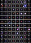 |
Fig. A.1. Pan-STARRS 3-color gri images of candidates with grades ≥2 from visual inspection of CNN scores pCNN > 0.9. See Fig. 9 caption. |
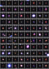 |
Fig. A.1. continued. |
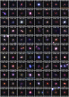 |
Fig. A.1. continued. |
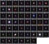 |
Fig. A.1. continued. |
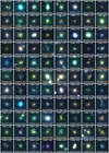 |
Fig. A.2. Legacy 3-color images of candidates covered in DR8. |
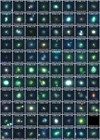 |
Fig. A.2. continued. |
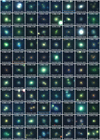 |
Fig. A.2. continued. |
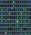 |
Fig. A.2. continued. |
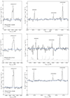 |
Fig. A.3. PS1 lens candidates with multiple emission lines from a high-redshift background galaxy overlaid on the SDSS BOSS spectrum of the foreground LRG. The black, gray and blue lines show the observed spectrum, the 1σ noise level, and the best-fit SDSS template for the LRG, respectively. The spectrum is zoomed on the spectral features associated with the background line-emitter rather than with the LRG. Top: PS1J2345−0209 with zLRG = 0.2940 and zs = 0.6581. Middle: PS1J1134+1712 with zLRG = 0.3752 and zs = 0.8121. Bottom: PS1J1724+3146 with zLRG = 0.2097 and zs = 0.3461. |
All Tables
Final list of galaxy-scale strong lens candidates with lens LRGs from our systematic search in Pan-STARRS.
All Figures
|
Fig. 1. Left: examples of strong gravitational lens systems mocked up by painting COSMOS lensed sources on PS1 stack images, and used as positive examples for training. Right: PS1 postage stamps of a subset of the 90 000 galaxies used as negative examples, including face-on spirals, massive LRGs, and field galaxies with similar gri colors as the mocks. All postage stamps are 20″ × 20″. |
| In the text | |
|
Fig. 2. Aperture magnitudes and colors of galaxies in the lens LRG catalog (red regions) and in the set of 90 000 mock lens systems (blue regions). The red and blue dots show the median of distributions. Left: (g − i) vs. i diagram for the R3 aperture, a circular aperture of 1.04″ radius. Right: difference in (g − i) color between the inner R3 aperture and concentric annuli between R3 and R4 (1.76″ outer radius), and between R4 and R5 (3.00″ outer radius). Gray regions mark the position of 100 000 random sources with reliable gri aperture photometry selected from the PS1 DR2 catalogs. Orange regions show galaxies with pcat > 0.5 on the catalog-level network, which match the colors and magnitudes of mocks lens systems. Solid and dashed lines show the 0.5, 1, and 2σ contours. |
| In the text | |
|
Fig. 3. Architecture of the convolutional neural network, inspired from LeNet (LeCun et al. 1998), and comprised of three convolutional layers with 11 × 11, 7 × 7, and 3 × 3 kernel sizes, and 32, 64, and 128 filters, respectively, followed by three fully connected hidden layers with 2048, 512, and 32 neurons. ReLU activations were applied between each layers. Max-pooling layers with 2 × 2 kernel sizes and stride = 2 were inserted after the first two convolutional layers, and dropout of 0.5 was used before the fully connected layers. |
| In the text | |
|
Fig. 4. Training of the CNN with optimized hyperparameters and using early stopping. The training loss (red curve) and validation loss (blue curve) were taken as the average of all cross-validation runs (light red and blue curves). |
| In the text | |
|
Fig. 5. Distribution of network predictions compared with the ground-truth for lenses (green) and nonlenses (orange) in the test set. |
| In the text | |
|
Fig. 6. Receiver Operating Characteristic curve for the trained CNN showing the true position rate (TPR) as function of the false positive rate (FPR) for different lens identification thresholds. The corresponding area under curve (AUC) is 0.985. |
| In the text | |
|
Fig. 7. Normalized distributions of CNN scores for mocks lenses included as positive examples in the test set, for different ranges of Einstein radii (left), θE/Reff (middle), and rKron (right). |
| In the text | |
|
Fig. 8. Three-color images of the 16 confirmed lens systems in the MasterLens database that have clear strong lensing signatures in Pan-STARRS images, and Einstein radii of 1–3″ similar to our mocks. The CNN scores are displayed at the top of each panel. Images are 15″ × 15″. |
| In the text | |
|
Fig. 9. Top: Pan-STARRS 3-color gri images of a subset of candidates with grades ≥2 from visual inspection of CNN scores pCNN > 0.9 (the complete figure is available in Appendix A). Numbers displayed on top of each panel are CNN scores (pCNN, left) and average visual grades (right). Candidates with PS1 names marked in orange have been previously published in the literature (see Table 1 and Sect. 6.1) Those marked in blue show unambiguous spectral signatures of high-redshift background sources in our inspection of SDSS BOSS DR16 data. Bottom: examples of random false positives with pCNN = 1. All cutouts are 15″ × 15″. |
| In the text | |
|
Fig. 10. Pan-STARRS lens candidate with prominent Balmer absorption features from a background galaxy at zs = 1.185 blended with the BOSS spectrum of the lens LRG at zd = 0.3155. The black and gray lines show the spectrum observed with a fiber of 2″ diameter and the 1σ noise level, respectively, and the blue line corresponds to the best-fit LRG template from the automated SDSS pipeline at λ < 8000 Å (see inset), which poorly fits the continuum and Balmer lines at longer wavelengths. The red line shows that combining the SED templates of an LRG at zd = 0.3155 (brown curve) and a recently quenched galaxy at zs = 1.185 (orange curve) correctly fits the spectrum over the entire range (see details in text). |
| In the text | |
|
Fig. 11. Example of a lens candidate with multiple emission lines from a high-redshift background galaxy overlaid on the SDSS BOSS spectrum of the foreground LRG. The black, gray and blue lines show the observed spectrum, the 1σ noise level, and the best-fit SDSS template for the LRG, respectively. The spectrum is zoomed on the spectral features associated with the background line-emitter at z = 0.8198 rather than with the LRG at z = 0.2386. |
| In the text | |
|
Fig. A.1. Pan-STARRS 3-color gri images of candidates with grades ≥2 from visual inspection of CNN scores pCNN > 0.9. See Fig. 9 caption. |
| In the text | |
|
Fig. A.1. continued. |
| In the text | |
|
Fig. A.1. continued. |
| In the text | |
|
Fig. A.1. continued. |
| In the text | |
|
Fig. A.2. Legacy 3-color images of candidates covered in DR8. |
| In the text | |
|
Fig. A.2. continued. |
| In the text | |
|
Fig. A.2. continued. |
| In the text | |
|
Fig. A.2. continued. |
| In the text | |
|
Fig. A.3. PS1 lens candidates with multiple emission lines from a high-redshift background galaxy overlaid on the SDSS BOSS spectrum of the foreground LRG. The black, gray and blue lines show the observed spectrum, the 1σ noise level, and the best-fit SDSS template for the LRG, respectively. The spectrum is zoomed on the spectral features associated with the background line-emitter rather than with the LRG. Top: PS1J2345−0209 with zLRG = 0.2940 and zs = 0.6581. Middle: PS1J1134+1712 with zLRG = 0.3752 and zs = 0.8121. Bottom: PS1J1724+3146 with zLRG = 0.2097 and zs = 0.3461. |
| In the text | |
Current usage metrics show cumulative count of Article Views (full-text article views including HTML views, PDF and ePub downloads, according to the available data) and Abstracts Views on Vision4Press platform.
Data correspond to usage on the plateform after 2015. The current usage metrics is available 48-96 hours after online publication and is updated daily on week days.
Initial download of the metrics may take a while.