| Issue |
A&A
Volume 688, August 2024
|
|
|---|---|---|
| Article Number | A34 | |
| Number of page(s) | 28 | |
| Section | Catalogs and data | |
| DOI | https://doi.org/10.1051/0004-6361/202449929 | |
| Published online | 02 August 2024 | |
TEGLIE: Transformer encoders as strong gravitational lens finders in KiDS
From simulations to surveys★
1
National Centre for Nuclear Research,
ul. Pasteura 7,
02-093
Warsaw,
Poland
e-mail: This email address is being protected from spambots. You need JavaScript enabled to view it.
2
Astronomical Observatory of the Jagiellonian University,
Orla 171,
30-001
Cracow,
Poland
3
Department of Physics and Astronomy, University of the Western Cape,
Bellville, Cape Town,
7535,
South Africa
4
South African Radio Astronomy Observatory,
2 Fir Street, Black River Park,
Observatory
7925,
South Africa
Received:
10
March
2024
Accepted:
16
May
2024
Abstract
Context. With the current and upcoming generation of surveys, such as the Legacy Survey of Space and Time (LSST) on the Vera C. Rubin Observatory and the Euclid mission, tens of billions of galaxies will be observed, with a significant portion (~105) exhibiting lensing features. To effectively detect these rare objects amidst the vast number of galaxies, automated techniques such as machine learning are indispensable.
Aims. We applied a state-of-the-art transformer algorithm to the 221 deg2 of the Kilo Degree Survey (KiDS) to search for new strong gravitational lenses (SGLs).
Methods. We tested four transformer encoders trained on simulated data from the Strong Lens Finding Challenge on KiDS data. The best performing model was fine-tuned on real images of SGL candidates identified in previous searches. To expand the dataset for fine-tuning, data augmentation techniques were employed, including rotation, flipping, transposition, and white noise injection. The network fine-tuned with rotated, flipped, and transposed images exhibited the best performance and was used to hunt for SGLs in the overlapping region of the Galaxy And Mass Assembly (GAMA) and KiDS surveys on galaxies up to z = 0.8. Candidate SGLs were matched with those from other surveys and examined using GAMA data to identify blended spectra resulting from the signal from multiple objects in a GAMA fiber.
Results. Fine-tuning the transformer encoder to the KiDS data reduced the number of false positives by 70%. Additionally, applying the fine-tuned model to a sample of ~5 000 000 galaxies resulted in a list of ~51 000 SGL candidates. Upon visual inspection, this list was narrowed down to 231 candidates. Combined with the SGL candidates identified in the model testing, our final sample comprises 264 candidates, including 71 high-confidence SGLs; of these 71, 44 are new discoveries.
Conclusions. We propose fine-tuning via real augmented images as a viable approach to mitigating false positives when transitioning from simulated lenses to real surveys. While our model shows improvement, it still does not achieve the same accuracy as previously proposed models trained directly on galaxy images from KiDS with added simulated lensing arcs. This suggests that a larger fine-tuning set is necessary for a competitive performance. Additionally, we provide a list of 121 false positives that exhibit features similar to lensed objects, which can be used in the training of future machine learning models in this field.
Key words: gravitational lensing: strong / methods: data analysis / catalogs
Full Table 6 is available at the CDS via anonymous ftp to cdsarc.cds.unistra.fr (130.79.128.5) or via https://cdsarc.cds.unistra.fr/viz-bin/cat/J/A+A/688/A34
© The Authors 2024
 Open Access article, published by EDP Sciences, under the terms of the Creative Commons Attribution License (https://creativecommons.org/licenses/by/4.0), which permits unrestricted use, distribution, and reproduction in any medium, provided the original work is properly cited.
This article is published in open access under the Subscribe to Open model. This email address is being protected from spambots. You need JavaScript enabled to view it. to support open access publication.
1 Introduction
Strong gravitational lensing is a general relativity-predicted phenomenon in which the potential of a massive foreground object, curving space-time, deflects the trajectory of the signal coming from a background source into separate multiple images. When the lens and the foreground object align along the line of sight, the common observation is either two or four images, forming the iconic Einstein cross around the deflector. Alternatively, arc-like structures can manifest, creating a nearly complete ring around the lens, commonly referred to as the Einstein ring.
Strong gravitational lensing is rarely observed as it depends on two objects aligning along the line of sight. This is reflected in the limited number of candidate strong gravitational lenses (SGLs) that have been discovered to date. A few thousand have been identified, but only a few hundred have been confirmed (e.g., Bolton et al. 2008; Brownstein et al. 2011; Tran et al. 2022).
Gravitational lensing is a valuable tool with a number of applications. For example, it can be used validate general relativity (Cao et al. 2017; Wei et al. 2022), constrain dark matter models (e.g., Dye & Warren 2005; Hezaveh et al. 2016), study the distribution of dark energy in the Universe (e.g., Collett & Auger 2014; Cao et al. 2015), and study the formation and evolution of galaxies (e.g., Barnabè et al. 2012; Nightingale et al. 2019).
Wide-area surveys like the Legacy Survey of Space and Time (LSST; LSST Science Collaboration 2009) and the Euclid mission (Laureijs et al. 2011) will collect an unprecedented volume of data, mapping about half of the sky (~20000 deg2). LSST is expected to observe ~20 billion galaxies, including ~105 galaxy–galaxy lenses and ~104 strongly lensed quasars (Verma et al. 2019). Euclid is expected to detect more than 105 SGL systems (Collett 2015). The sheer volume of galaxies observed in these surveys, coupled with the relatively low occurrence of SGLs, render manual identification of SGLs prohibitively time-consuming and inefficient, necessitating the development of automated detection algorithms. Nonetheless, every SGL detected by an automated technique requires visual inspection by an expert to confirm its validity as a candidate. For conclusive confirmation, spectroscopic follow-up observations are required. Although crowd-sourcing initiatives such as Space Warps have proved useful in identifying SGL candidates in the past (More et al. 2015; Marshall et al. 2016; Sonnenfeld et al. 2020; Garvin et al. 2022), the ever-increasing volume of observational data renders the approach of presenting all sources to volunteers unsustainable. Some successful automated methods for the detection of SGL-like features have been proposed, such as ARCFINDER (Seidel & Bartelmann 2007) or RingFinder. More recently, these algorithms, although shown to be effective in SGL detection, have been outperformed by more sophisticated machine learning (ML) methods in recent SGL detection challenges (Metcalf et al. 2019). Machine learning algorithms have thus appeared as a promising tool for automatically detecting SGL candidates. Their application has already led to the identification of thousands of SGL candidates in surveys such as the Kilo Degree Survey (KiDS; Petrillo et al. 2017, 2018, 2019; Li et al. 2020, 2021; He et al. 2020), Dark Energy Camera Legacy Survey (DECaLS; Huang et al. 2020, 2021; Stein et al. 2022; Storfer et al. 2022), VLT Survey Telescope (VST; Gentile et al. 2021), Panoramic Survey Telescope and Rapid Response System (Pan-STARRS; Canameras et al. 2021), Dark Energy Survey (DES; Diehl et al. 2017; Jacobs et al. 2019; Rojas et al. 2022; O’Donnell et al. 2022; Zaborowski et al. 2023), Low-Frequency Array (LOFAR; Rezaei et al. 2022) and Hyper Suprime-Cam (HSC; Canameras et al. 2021; Shu et al. 2022).
In much of the aforementioned research, convolutional neural networks (CNNs) have emerged as the preferred architecture for SGL identification. Notably, a CNN model secured the top performance in the SGL Finding Challenge (Metcalf et al. 2019). CNNs are supervised ML gradient-based algorithms first introduced by LeCun et al. (1998) for handwritten digit recognition. Since their debut, CNNs have revolutionized the field of image recognition (Krizhevsky et al. 2012; Simonyan & Zisserman 2015; He et al. 2016; Szegedy et al. 2015; Huang et al. 2017; Tan & Le 2019). CNNs had for years been the state-of-the-art tool for object recognition, until the recent breakthrough in natural language processing (NLP) with the introduction of a new self-attention-based architecture, known as transformers (Vaswani et al. 2017). This architecture’s significant impact on NLP is evidenced by models like BERT, developed by researchers at Google AI (Devlin et al. 2019), which uses a bidirectional encoding approach, considering both the left and right context of a word during training, unlike its predecessors. At the time of its release, BERT had achieved state-of-the-art performance on a wide range of NLP tasks, including text classification, question answering, and text summarization (e.g., Wang et al. 2019). At the core of transformers lies the attention mechanism, which dynamically assigns varying weights to different parts of the input data, enabling the model to prioritize relevant information and model long-range dependences.
The attention mechanism has been successfully extended to image analysis (Carion et al. 2020; Dosovitskiy et al. 2021; Yu et al. 2022; Wortsman et al. 2022), and transformers have proven to be more robust learners than CNNs (Paul & Chen 2022). Beyond their success in image classification and object detection, transformers have also proven adept at various image processing tasks, including image segmentation, image superresolution, and image restoration (Khan et al. 2022; Aslahishahri et al. 2023; Li et al. 2023). The astronomical community has rapidly recognized the potential of transformers, leading to a variety of applications (Merz et al. 2023; Donoso-Oliva et al. 2023; Allam & McEwen 2023; Hwang et al. 2023; Thuruthipilly et al. 2024b), including strong lens detection (Thuruthipilly et al. 2022, 2024a; Huang et al. 2022; Jia et al. 2023).
Supervised ML models require a substantial amount of labeled data, typically in the range of tens of thousands of samples, to attain optimal performance. However, for rare phenomena such as SGLs, where only a few thousand lens candidates have been identified and observations are restricted to specific instruments, large labeled datasets are not readily available. To address this challenge, artificial datasets with lens systems as realistic as possible are generated employing various techniques. Mimicking the complex morphology of lens systems is a challenging task, and creating realistic examples of non-lenses is equally difficult. Irregular galaxies, mergers, and ring galaxies can all exhibit features that resemble those of SGLs. For these reasons, transitioning from a simulated dataset to real-world SGL searches invariably results in an increase in false positives (FPs) compared to the numbers encountered during training with artificial data. However, when moving from simulated datasets to real-world data, where non-lenses vastly outnumber lenses, final visual inspection remains indispensable for validation.
This study examines the potential of transformers to detect SGLs, the role of sample selection by galaxy type, and the impact of fine-tuning in reducing FPs. We also investigate different data augmentation techniques for increasing the fine-tuning dataset size. Examining FPs, the primary reason models achieve lower accuracy, is crucial for building robust training sets. This analysis helps us understand model shortcomings and guides the development of more accurate training data, especially considering the vast number of galaxies that next-generation surveys will detect.
The transformers we use are described in Thuruthipilly et al. (2022) and were trained on the simulated Bologna Strong Lens Finding Challenge dataset (Metcalf et al. 2019). The best-performing fine-tuned model is supplied with images from where KiDS and Galaxy And Mass Assembly (GAMA) footprints overlap.
The paper is structured as follows: Sec. 2 examines the previous SGL searches in KiDS. Section 3 introduces the data and outlines the preprocessing criteria used to select the sample. The methodology adopted in this work is detailed in Sec. 4. Section 5 presents a comprehensive evaluation of various transformers to assess their performance in detecting strong lenses on KiDS images. Section 6 characterizes the newly discovered lenses, introducing the Transformer Encoders as strong Gravitational Lens finders In the kilo-degreE survey (TEGLIE) for this sample. Section 8 delves into the properties of the TEGLIE lenses. Section 9 provides an analysis of the results, while Sect. 10 summarizes the main findings and highlights the potential of ML for SGL detection.
2 Previous strong lens searches in KiDS with CNNs
KiDS, with its extensive size and depth, provides an ideal testing ground for the application of ML techniques to the detection of SGLs, as demonstrated by previous studies (Petrillo et al. 2017, 2018, 2019; Li et al. 2020, 2021). All of these searches have been conducted using CNN architectures. For this reason, we investigated the effectiveness of the current state-of-the-art methods for image classification on terrestrial images, namely self-attention-based models, in detecting rare astronomical objects such as SGLs within KiDS.
In order to provide an adequate context for our subsequent analyses, we present a brief overview of the SGL searches that have been conducted as part of KiDS. This comparative perspective will prove useful when evaluating different approaches and sample selection strategies in the following sections.
Initial studies by Petrillo et al. (2017, 2018) used a CNN to identify SGLs within luminous red galaxies (LRGs) extracted from KiDS DR3. The network was trained on simulated SGL images created by superimposing simulated lensed images on real LRGs observed in the survey. Subsequent studies by Petrillo et al. (2019); Li et al. (2020, 2021) further refined the approach by extending the target set to include bright galaxies (BGs) in addition to LRGs from DR4 and DR5 (not yet publicly available). Both LRGs and BGs are massive galaxies with a large lensing cross-section, making them prime candidates for SGL detection (Oguri & Marshall 2010). Since LRGs are a subset of BGs by definition, the target dataset undergoes a preliminary selection process to identify specific BGs. In all the KiDS SGL searches, the galaxies meeting the following criteria were considered to be BGs.
SExtractor r-band Flag < 4, to eliminate objects with incomplete or corrupted photometry, saturated pixels, extraction, or blending issues.
IMA_FLAGS = 0, excluding galaxies in compromised areas.
SExtractor Kron-like magnitude MAG_AUTO, in the r band, rauto ≤ 21 mag, maximizing the lensing cross-section (Schneider et al. 1992).
KiDS star-galaxy separation parameter SG2DPHOT = 0, selecting galaxy-like objects. This parameter has values of 1 for stars, 2 for unreliable sources, 4 for stars based on star galaxy separation criteria, and 0 for nonstellar objects. For further details refer to La Barbera et al. (2008); de Jong et al. (2015); Kuijken et al. (2019).
From the BG sample, LRGs are extracted by imposing two further criteria, (1) rauto ≤ 20 mag and (2) color-magnitude selection at low redshift (z < 0.4) based on Eisenstein et al. (2001), with some modifications to include fainter and bluer sources:
![Mathematical equation: $\[\begin{aligned}& \left|c_{\text {perp }}\right|<0.2 \\& r_{\text {auto }}<14+c_{\text {par }} / 0.3,\end{aligned}\]$](/articles/aa/full_html/2024/08/aa49929-24/aa49929-24-eq1.png) (1)
(1)
where
![Mathematical equation: $\[\begin{aligned}& c_{\text {par }}=0.7(g-r)+1.2[(r-i)-0.18] \\& c_{\text {perp }}=(r-i)-(g-r) / 4.0-0.18\end{aligned}.\]$](/articles/aa/full_html/2024/08/aa49929-24/aa49929-24-eq2.png) (2)
(2)
In Petrillo et al. (2017), a CNN was used to identify SGLs from a sample of 21 789 LRGs in KiDS DR3, yielding 761 SGL candidates. After visual inspection, 56 of these candidates were deemed reliable. Similarly, Petrillo et al. (2019) used two CNNs to search for SGLs between the LRG galaxies in KiDS DR4. The CNNs, using r-band images and g, r, and i color-composited images as input, detected 2510 and 1689 candidates, respectively, from a sample of 88 327 LRGs. After visual inspection, these candidates were narrowed down to 1983 potential SGLs and 89 strong high-quality (HQ) candidates. This catalog of Lenses in the KiDS survey (LinKS) is publicly available1.
Li et al. (2020, 2021) extended the target sample to include both BGs and LRGs from DR4 and DR5, respectively. In their study, Li et al. (2020) employed the same CNN architecture as in Petrillo et al. (2019), taking as input only r-band images, to a sample of 3 808 963 BGs and 126 884 LRGs. This CNN successfully identified 2848 SGL candidates among the BGs and 3552 candidates among the LRGs. After visual inspection, 133 BG and 153 LRG candidates were classified as high-probability SGLs.
In subsequent work, Li et al. (2021) employed two different CNN architectures to analyze the 341 deg2 of the KiDS final unpublished release (DR5). The first CNN, which takes as input r-band images, identified 1213 SGL candidates, and the second CNN, which takes as input g, r, and i color-composited images, identified 1299 candidates. Visual inspection deemed the candidates to be 487, with 192 BG and 295 LRG candidates classified as high-probability SGLs. Among these high-probability SGLs, 97 were selected as the most likely SGL candidates. The full HQ SGL catalog from these studies is available on the KiDS DR4 website2.
3 Data
3.1 Kilo-Degree Survey
The KiDS (de Jong et al. 2013, 2015, 2017; Kuijken et al. 2019) is a European Southern Observatory (ESO) public widefield medium-deep optical four-band imaging survey with the main aim of investigating weak lensing. It is carried out with an OmegaCAM camera (Kuijken 2011) mounted on the VST (Capaccioli & Schipani 2011) at the Paranal Observatory in Chile. The OmegaCAM has a 1 deg2 of field of view and the pixels have an angular scale of 0.21″. The r band has the best seeing, the point spread function (PSF) full width at half maximum is 1.0, 0.8, 0.65, and 0.85 arcsec in the u, g, r, and i bands, respectively (de Jong et al. 2015, 2017). The source extraction and the associated photometry have been obtained by the KiDS collaboration using SExtractor (Bertin & Arnouts 1996) and the multiband colors are measured by the Gaussian Aperture and PSF (GAaP) code (Kuijken 2008).
The latest publicly available release of KiDS is Data Release 4 (Kuijken et al. 2019), encompassing 10006 tiles covering approximately 1000 deg2 of the sky. With the upcoming final data release (DR5) becoming public, the KiDS dataset will cover approximately 1350 deg2 of the sky in the four optical bands, u, g, r, and i.
3.2 KiDS sample selection
For this study, we utilized a subset of KiDS DR4, comprising 221 tiles (~220 deg2) that all overlap with the GAMA spectroscopic survey footprint. The GAMA regions overlapping with KiDS are detailed in Table 1. Within the survey regions G09, G12, G15, and G23, there are 56, 56, 60, and 49 tiles in KiDS DR4, respectively. Future studies could model the newly discovered lenses by leveraging a combination of GAMA spectroscopic redshifts and other measurements with the KiDS images, adopting an approach similar to that employed in Knabel et al. (2023).
In line with the approach employed in previous SGL searches, as discussed in Sec. 2, we restricted our target to sources with an r-band Flag value less than 4. Additionally, to minimize contamination from galaxies in compromised regions such as reflection halos and diffraction spikes, we only considered sources with a ima_flags value of zero in all bands. In contrast to previous studies that employed a Kron-like magnitude threshold of rauto < 21 mag (Li et al. 2020, 2021; Petrillo et al. 2017, 2018, 2019), we extended our target sample to include all galaxies with photometric redshifts up to z = 0.8, without putting any limit on rauto. This allows for a more comprehensive exploration of the lensing population and potentially identifies fainter SGLs.
The photometric redshifts for the target sample are obtained from the KiDS DR4 catalog using the Bayesian photometric redshift (BPZ) code (Benítez 2011). For redshift selection, the focus is on Z_B, an estimate of the most probable redshift from the nine-band images (peak of the posterior probability distribution), Z_ML, the nine-band maximum likelihood redshift, and the lower and upper bounds of the 68% confidence interval of Z_B. Objects with estimated redshifts Z_B and Z_ML within the 0.0–0.8 redshift range are included, and additionally Z_ML is required to fall within the lower and upper 1σ bounds of Z_B, ensuring that the redshift estimates are consistent and reliable.
We aim to identify lenses that may have been overlooked in previous searches, including those where the lens and lensed objects are in close proximity. Therefore, we refrained from imposing any constraints on the star-galaxy separation parameter SG2DPHOT, which flags celestial objects as stars based on the source r-band morphology. However, in future studies, it may be crucial to impose constraints on this parameter to optimize computational efficiency.
This sample selection limits the sample to 5 538 525 elements out of 21 950 980 within the 221 KiDS tiles. For the image cutouts, we selected dimensions of 101 × 101 pixels, corresponding to 20″ × 20″ in KiDS. These square regions were centered on the centroid sky position derived from the r-band co-added image of the target galaxy. The cutout size corresponds to 90 kpc × 90 kpc at z = 0.3 or 120 kpc × 120 kpc at z = 0.5 (Li et al. 2020).
GAMA survey regions.
3.3 Synthetic KiDS-like data
The Bologna Strong Gravitational Lens Finding Challenge3 (Metcalf et al. 2019), a now-concluded open challenge, tasked participants with developing automated algorithms to identify SGLs among other types of sources. The mock galaxies were generated within the Millennium simulation (Boylan-Kolchin et al. 2009) and lensed using the GLAMER lensing code (Metcalf & Petkova 2014; Petkova et al. 2014). The challenge dataset consisted of 85% purely simulated images and 15% real images of BGs from KiDS. Lensing features were added to both samples with a rate of 50%. The challenge dataset comprises 100 000 images while the training set consists of 20 000 images, each measuring 101 × 101 pixels. These images have been created to mimic the noise levels, pixel sizes, sensitivities, and other parameters of KiDS. The images encompass four bands, designated as (u, g, r, and i), with the r band serving as the reference band. The image resolution is 0.2″, which results in a 10″ × 10″ image.
3.4 GAMA spectroscopy and AUTOZ redshifts
The GAMA survey (Driver et al. 2009, 2011, 2022; Liske et al. 2015) is a multiwavelength spectroscopic survey conducted using the Anglo-Australian Telescope’s spectrograph. GAMA Data Release 4 (Driver et al. 2022) provides redshifts for over 330000 targets spanning over ~250 deg2. These redshifts are determined through a fully automated template-fitting pipeline known as AUTOZ (Baldry et al. 2014). AUTOZ is capable of identifying spectral template matches that may contain contributions from two distinct redshifts within a single spectrum. In addition to the redshift, the algorithm retrieves cross-correlation redshifts against a library of stellar and galaxy templates. The galaxy templates (numbered 40 to 47 in order of increasing emission-line strength) are broadly categorized as passive galaxies (PGs) for templates 40–42 and emission-line galaxies (ELGs) for templates 43–47, with lower-numbered templates corresponding to stars (Holwerda et al. 2015). Based on the best-fit galaxy type at each redshift component, it is possible to classify the blended galaxies. These classifications include two passive galaxies (PG+PG), two emission-line templates (ELG+ELG), a passive galaxy at a lower redshift and an emission-line galaxy at a higher redshift (PG+ELG), or the inverse scenario (ELG+PG).
The public online catalog AATSpecAutozAllv27_DR44 provides the outputs of the AUTOZ algorithm. The catalog includes the best-fitting galaxy template and the four flux-weighted cross-correlation peaks (σ) of redshift matches with galaxy templates. The highest peak (σ1) corresponds to the best-fit redshift, while subsequent peaks have progressively lower correlation values with σ4 having the weakest correlation.
Holwerda et al. (2015) used the outputs from AUTOZ to compile a catalog of blended galaxy spectra within GAMA DR2 (Liske et al. 2015). Blended spectra arise when the light from two distinct galaxies falls within the same GAMA fiber. Consequently, cases where two separate galaxy templates provide high-fidelity matches, yet yield significantly different redshifts, are indicative of potential blended sources. These blended sources can be attributed to either strong gravitational lensing events or serendipitous overlaps of two galaxies along the line of sight. To quantify the strength of the secondary redshift candidates, Holwerda et al. (2015) selected double-z candidates via the ratio R:
![Mathematical equation: $\[R=\frac{\sigma_2}{\sqrt{\sigma_3 / 2+\sigma_4 / 2}},\]$](/articles/aa/full_html/2024/08/aa49929-24/aa49929-24-eq3.png) (3)
(3)
where σ2 represents the second highest redshift peak value, and σ3 and σ4 the third and fourth peaks, respectively. This ratio allows for the selection of candidate redshifts with prominent secondary peaks compared to the remaining two.
Holwerda et al. (2015) adopted a threshold of R > 1.85 along with the requirement of foreground+background galaxy pairs as PG+ELG for identifying SGL candidates because it was the most observed configuration of the Sloan Lens ACS Survey (SLACS) strong lenses confirmed with Hubble Space Telescope (HST) (e.g. Bolton et al. 2008; Shu et al. 2017). After visually inspecting the images of candidates in the Sloan Digital Sky Survey (SDSS) and KiDS, Holwerda et al. (2015) obtained 104 lens candidates and 176 occulting galaxy pairs.
Knabel et al. (2023) employed a similar strategy for selecting strong lensing candidates by analyzing GAMA spectra. They examined the spectra of candidates previously identified during SGL searches within KiDS (Petrillo et al. 2019; Li et al. 2020). Since the KiDS collaboration preselected these candidates, Knabel et al. (2023) used a less stringent threshold on R (R ≥1.2) compared to Holwerda et al. (2015). Additionally, they required a foreground source redshift exceeding 0.5. Following this selection, 42 candidates were chosen for further analysis and modeling using the PYAUTOLENS software (Nightingale et al. 2019). Among these, 19 candidates yielded successful modeling results. While the majority exhibited PG+ELG galaxy configurations, other configurations were also present.
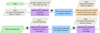 |
Fig. 1 Schematic view of this work’s methodology. The eye icon denotes the process of visually evaluating ML candidates, and T+22 stands for Thuruthipilly et al. (2022). The comprehensive details of each step in this flowchart are presented in Sec. 4. |
4 Methodology
In a recent publication, Thuruthipilly et al. (2022) used, for the first time, transformer encoders (TEs) to identify SGLs. A total of 18 000 images from the Lens Challenge dataset (see Sec. 3.3) were used to train 21 different TEs. This section outlines the TE architectures, performance metrics, and fine-tuning approach used in our study. A comprehensive overview of our methodology can be found in Fig. 1. The best-performing weights (before and after fine-tuning) and architecture of the model are publicly available on GitHub5.
4.1 The transformer encoder model
Figure 2 presents a schematic view of the transformer employed in this work. The initial component is a simple CNN designed to extract pertinent features from the input image. Since the transformer architecture is permutation-invariant, a fixed positional encoding is incorporated into the output of the CNN backbone. The positional encoding is defined as (Vaswani et al. 2017)
![Mathematical equation: $\[P E_{(\mathrm{pos}, 2 i)}=\sin \left(p o s / 12~800^{\frac{2 i}{d_{\text {model }}}}\right)\]$](/articles/aa/full_html/2024/08/aa49929-24/aa49929-24-eq4.png) (4)
(4)
![Mathematical equation: $\[P E_{(\mathrm{pos}, 2 i+1)}=\cos \left(p o s / 12~800^{\left.\frac{2 i}{d_{\text {model }}}\right)}\right),\]$](/articles/aa/full_html/2024/08/aa49929-24/aa49929-24-eq5.png) (5)
(5)
where pos is the position, i is the dimension of the positional encoding vector, and dmodel is the dimension of the input feature vector. The positional encoding layer embeds the positional information of each feature into the representation. This information is essential for the model to understand the spatial context of the features.
The features, along with their positional encoding, are then fed into the TE layer, which comprises a multi-head self-attention module and a feed-forward network (FFN). Within this layer, self-attention is applied to the input. This process involves treating each point in the feature map as a random variable and determining the pairwise covariances. The value of each prediction is enhanced or diminished based on its similarity to other points in the feature map. The FFN learns the weighted features filtered by the encoder layers.
The model output is a single neuron with a sigmoid activation function that predicts the likelihood of the input image being a lens. This value, known as the prediction probability, ranges from 0 to 1, with 1 representing the maximum probability of the image containing a lens. We considered all elements with a prediction probability exceeding 0.8 as lens candidates.
In this work, we employed the three best-performing models (M15, M16, M21) trained on four-band simulated images by Thuruthipilly et al. (2022) and one model specifically trained on r, i, g-band images (RIG model). The incorporation of the three-band model stems from the observation that the u-band data in the real KiDS images exhibit significantly poorer seeing conditions. Consequently, a three-band network could potentially show superior performance on real data. Furthermore, previous searches in KiDS primarily employed three- or one-band networks.
Table 2 summarizes the model architectures. In a TE, the notation X HY indicates the presence of X independent attention heads, each processing a hidden representation of dimension Y. These heads act as multiple independent units focusing on different aspects of the data. The dimension, Y, refers to the size of the hidden representation processed by each head and determines the model’s complexity and capacity. Furthermore, Z(E) denotes the inclusion of Z, the main processing units that extract information from the input data and pass it through subsequent layers. The area under the receiver operating characteristic curve (AUROC), true positive rate (TPR), and false positive rate (FPR) metric definitions are provided in Appendix B.
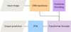 |
Fig. 2 Scheme of the general architecture of the TE. The extracted features of the input image by the CNN backbone are combined with positional encoding and passed on to the encoder layer to assign attention scores to each feature. The weighted features are then passed to the feed-forward neural network to predict the probability. |
Name, model structure, AUROC, TPR, and FPR of the models from Thuruthipilly et al. (2022) used in this study.
4.2 Metrics
Astronomical surveys like KiDS lack precise counts of genuine lenses and non-lenses within the data. While visual inspection allows us to identify correctly classified lenses – the true positives (TPs) – and non-lenses misidentified as lenses (FPs), it is difficult to determine the exact number of missed lenses as well as the correctly classified non-lenses. This limitation renders commonly used evaluation metrics, such as AUROC, TPR, and FPR, inapplicable.
To assess our models’ performance, we instead used the precision metric:
![Mathematical equation: $\[P=\frac{\mathrm{TP}}{\mathrm{TP}+\mathrm{FP}}.\]$](/articles/aa/full_html/2024/08/aa49929-24/aa49929-24-eq6.png) (6)
(6)
4.3 Visual inspection
Visual inspection is a valuable, albeit time-consuming, step for preliminary quality assessment of candidate lenses identified by the ML model. This step is essential for obtaining a clean training dataset and estimating model precision.
The individual tasked with evaluating the candidate images, referred to as the inspector, is presented with four bands of 101 x 101 pixel images and a composite red-green-blue image constructed from the r, i, and g bands, as outlined in the methodology presented in Lupton et al. (2004). The inspector is then required to assign a grade to the object displayed on the screen. The available options are as follows:
0: No lensing features are present
1: Most likely a SGL. The presence of clear lensing features, such as arcs or multiple distorted images, strongly suggests strong gravitational lensing. Accordingly, grade 1 was assigned to candidates with blue arcs and a red source or when multiple images were positioned in a manner consistent with strong gravitational lensing.
2: Possibly a SGL. The presence of a single image or a weakly curved arc-like structure raises the possibility of gravitational lensing. However, the absence of a distinct ring or the ambiguity between an Einstein ring and a ring galaxy hinders conclusive classification. This grade was awarded when only a single faint blue arc or image was visible and the configuration of the lens and source remained unclear.
3: Object exhibiting lensing-like features (arc-like structures) without being a lens: This grade was assigned to candidates that exhibited arc-like structures but were not caused by gravitational lensing. Such objects could be merging galaxies or unusual galaxies with peculiar structures.
The utility of a model hinges on the balance between TPs and FPs that is deemed acceptable by the inspectors. In the context of wide-area surveys, visual inspection represents a bottleneck in candidate identification, necessitating the implementation of a model with a relatively low FPR. Despite the unknown total number of strong lenses (TPs + FPs), the model’s performance can be assessed by evaluating its ability to identify lenses discovered by other surveys.
As previously stated, visual inspection is a time-consuming task. Due to the broad redshift range and lack of specific galaxy population restrictions in this study, only one expert initially assesses the candidates. Subsequently, a group of experts scrutinizes the more promising candidates (labeled 1, 2, or occasionally 3). The lenses retained with a grade of 1 after this final round are designated as HQ or high-confidence candidates, while all candidates (labeled 1 and 2) are referred to as TEGLIE candidates.
4.4 Fine-tuning and data augmentation
The Lens Finding Challenge dataset has been created for the purpose of testing different automated techniques for the identification of SGLs. Consequently, the dataset was not intended to precisely replicate real observations; rather, KiDS was employed as a guideline for image creation. For this reason, for instance, Davies et al. (2019) identified inconsistencies, such as an over-representation of large Einstein rings and simulated lensed galaxies fainter than the COSMOS lenses (Faure et al. 2008). Given the discrepancies observed, it is anticipated that models trained exclusively on the simulated dataset will exhibit suboptimal performance when presented with actual KiDS observations. Consequently, in order to mitigate this issue, the model with the highest performance is selected by evaluating it on a representative subset of KiDS data (10 deg2). Furthermore, transfer learning and data augmentation techniques are employed to enhance the training data, with the objective of fine-tuning the model to the characteristics of KiDS.
Transfer learning involves fine-tuning a model that has already been trained on a large, diverse dataset to adapt it to a specific task or domain. Previous studies have demonstrated the effectiveness of transfer learning in improving the performance of ML models on small datasets (Pan & Yang 2010; Yosinski et al. 2014). Instead of simply fine-tuning specific layers, we loaded the pretrained weights and fine-tuned the entire model on a representative subset of real KiDS data augmented to address the model’s limitations. In this approach, the knowledge learned from the simulated data is adapted to the unique features and characteristics present in real KiDS observations, potentially overcoming the challenge of identifying FPs.
Data augmentation refers to techniques that artificially expand the training set size by generating new images from the existing ones. Common approaches include geometric transformations (scaling, rotation, cropping, flipping), random erasing, noise injection, color space modifications, and many more. An in-depth overview of image augmentation techniques is available in Mumuni & Mumuni (2022) and Xu et al. (2023). However, the ideal augmentation strategy depends heavily on the specific model and task. Therefore, we used the best-performing model on the small KiDS data sample to test different combinations of augmentation techniques specifically for SGLs in KiDS. This process ensured we tailored the augmented data to the model’s needs, optimizing its ability to generalize to real-world observations. Ultimately, the model fine-tuned on the dataset yielding the best performance with data augmentation is selected to search for lenses in a larger KiDS area of ~200 deg2.
The dataset used for fine-tuning includes a balanced quantity of real observations of both SGLs and non-SGLs; the SGL class has few available examples and is therefore the only one that includes augmented images.
For the SGL class, 169 HQ strong lens candidates from KiDS DR4, identified by Petrillo et al. (2019); Li et al. (2020, 2021) and publicly available on the KiDS DR4 website6, are employed. Some of these previously discovered lenses used for fine-tuning are shown in Fig. 3.
In this work we used straightforward image augmentation techniques, including rotation, flipping, transposing, and noise injection. To preserve the intrinsic properties of the observed objects, we avoided transformations that alter the image’s color or zoom ratio. Specifically, we used rotation angles of 90°, 180°, and 270°, which are necessary to avoid empty corners. For noise injection, we introduced white Gaussian (![Mathematical equation: $\[\boldsymbol{\mathcal{N}}\]$](/articles/aa/full_html/2024/08/aa49929-24/aa49929-24-eq7.png) ) noise with a mean μ = 0 and standard deviations of σ = 10−11 and 10−15. To determine these values, we randomly selected 1000 cutouts that pass our sample selection. For each cutout, we calculated the average, minimum, and maximum pixel values. We then calculated the average of these three measurements, obtaining a minimum average value of −5.767 × 10⁻¹¹, a maximum average value of 2.644 × 10⁻⁹, and an average of 1.846 × 10⁻¹¹. We chose a noise level of the same order of magnitude as the average pixel value and a significantly smaller value to assess the network’s response to both magnitudes. An example of a SGL with different data augmentations is shown in Fig. 4.
) noise with a mean μ = 0 and standard deviations of σ = 10−11 and 10−15. To determine these values, we randomly selected 1000 cutouts that pass our sample selection. For each cutout, we calculated the average, minimum, and maximum pixel values. We then calculated the average of these three measurements, obtaining a minimum average value of −5.767 × 10⁻¹¹, a maximum average value of 2.644 × 10⁻⁹, and an average of 1.846 × 10⁻¹¹. We chose a noise level of the same order of magnitude as the average pixel value and a significantly smaller value to assess the network’s response to both magnitudes. An example of a SGL with different data augmentations is shown in Fig. 4.
The non-lens class in our dataset consists of images misclassified as strong lenses by the model. To improve its performance, we prioritized images with the highest probability of being misclassified lenses, a process known as uncertainty sampling (Lewis & Gale 1994). This technique identifies examples where the model exhibits the most uncertainty, allowing for efficient learning with minimal labeling effort. In our case, we have a fixed number of SGL candidates but a larger pool of non-lens examples. Therefore, we utilized all SGL candidates while selecting the most uncertain non-lens images based on their prediction error. This least confident sampling strategy prioritizes the most informative examples for model improvement. Specifically, we gathered the 150 most uncertain FP images from each of ten randomly selected KiDS DR4 tiles, ensuring equal representation from each tile. Figure 5 showcases some of these particularly uncertain non-lenses.
The datasets investigated in the fine-tuning process are
No augmentation: cutouts of SGL candidates found by the KiDS collaboration.
Rotated (R): four images for every SGL, the original plus the three rotations.
Rotated + Gaussian noise μ = 0, σ = 10−11: the rotated images described above but with some additional white noise drawn by
![Mathematical equation: $\[\boldsymbol{\mathcal{N}}\]$](/articles/aa/full_html/2024/08/aa49929-24/aa49929-24-eq8.png) (0, 10−11).
(0, 10−11).Rotated + Gaussian noise μ = 0, σ = 10−15: similar to the dataset described above, rotated images with additive white noise drawn from
![Mathematical equation: $\[\boldsymbol{\mathcal{N}}\]$](/articles/aa/full_html/2024/08/aa49929-24/aa49929-24-eq9.png) (0, 10−15).
(0, 10−15).Rotated, rotated + Gaussian noise μ = 0, σ = 10−15: rotated images and rotated images with additive noise drawn from
![Mathematical equation: $\[\boldsymbol{\mathcal{N}}\]$](/articles/aa/full_html/2024/08/aa49929-24/aa49929-24-eq10.png) (0, 10−15).
(0, 10−15).Rotated, flipped (RF): rotated images, and for every cutout, the flipped SGL with respect to the x-axis.
Rotated, flipped, transposed (RFT): rotated images, flipped SGL with respect to the x-axis, and transposed original image.
For each dataset, we randomly partitioned the data into training, testing, and validation sets, maintaining the equal representation of lenses and non-lenses classes. The test set comprises 20% of the overall augmented dataset, while the validation set constitutes 10% of the training set, leaving the remaining 72% of the augmented dataset for the training set. The sizes of the augmented datasets are presented in Table 3.
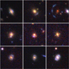 |
Fig. 3 Selection of the exemplary strong lens candidates found by the KiDS collaboration in DR4 (Li et al. 2020; Petrillo et al. 2019) and implemented in the fine-tuning dataset. |
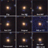 |
Fig. 4 High-quality KiDS SGL candidate (ICRS coordinates J030540.105-293416) cutout with different data augmentations. |
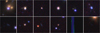 |
Fig. 5 Examples of cutouts employed as non-lenses in the fine-tuning dataset. |
Test and training set sizes for the different kinds of data augmentations.
5 Model evaluation
5.1 Testing on KiDS DR4
Table 2 summarizes the performance of the three best-performing models by Thuruthipilly et al. (2022). These models are tested on ten randomly selected KiDS tiles, listed in Table 4, none of these overlap with GAMA. The cutouts fed into the models are preprocessed according to the procedure described in Sec. 3.2. The distribution of prediction probabilities for each model across the ten tiles is depicted in the left plot of Fig. 6. The cutouts with a prediction probability exceeding the threshold of 0.8 (black vertical line in the figure) are referred to as ML candidates. To illustrate the proportion of TPs (blue bars) to FPs (purple bars), the candidates confirmed after visual inspection (TEGLIE candidates) are represented in the right plot of Fig. 6. The HQ (grade 1) candidates identified during this testing process have IDs ranging from 0 to 4 in Fig. 10 and Table A.1.
In the ten test tiles, 238 028 elements pass the preprocessing stage and are presented to the models. The precision of the different models is illustrated in Fig. 7. Compared to the other models, Model 16 identifies significantly fewer candidates (MLcandM16 = 4026), while Model 15 identifies the most candidates (MLcandM15 = 9944). Models 21 and RIG identify MLcandM21 = 7882 and MLcandRIG = 6100, respectively. Of these, TPM21 = 6 and TPRIG = 3 are visually confirmed as SGL candidates.
Model 15 achieves the highest precision PM15 = 0.11% among the models, followed by model 16 of PM16 = 0.099%, model 21 with PM21 = 0.076%, and model RIG with PRIG = 0.049%. Despite its high precision, Model 15 also generates double the number of FP compared to Model 16.
Figure 8 illustrates the overlap between the three models in terms of the candidates detected. The top diagram depicts the overlap for all candidates, while the bottom diagram represents the overlap for confirmed candidates. Given model RIG’s inferior performance, it has been excluded from this analysis. The three models identify distinct candidates, yet Model 15 uncovers the majority of the candidates found by Models 21 and 16. This indicates that Model 15 possesses a more comprehensive grasp of the shared characteristics of SGLs compared to the other two models.
The substantial prevalence of FPs renders the SGL detection impractical, necessitating fine-tuning. To accomplish this, one of the presented models must be selected. Model 15 exhibits the highest P among all models, despite having the highest number of FPs. Model 15 also has a significant overlap with the other models in terms of the detected candidates. This implies that Model 15 is capable of identifying a broad spectrum of SGL candidates and does not simply rely on a small number of very specific features. Additionally, Model 15 has demonstrated effectiveness on simulated data (Thuruthipilly et al. 2022), indicating that it is a robust model that is likely to generalize well to new datasets. Based on this assessment, Model 15 stands out as the most appropriate candidate for fine-tuning for KiDS.
Ten randomly chosen KiDS tiles used for testing the transformers on the survey data.
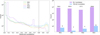 |
Fig. 6 Prediction probability sample extracted from the ten tiles in Table 4. Left: prediction probability of the four models used in this work from Thuruthipilly et al. (2022). The black line shows the threshold probability; every object above 0.8 is considered an ML candidate. Right: total number of ML candidates compared to the TPs with grades 1 and 2 (TEGLIE candidates) for every model. Bar element counts are shown above each bar. |
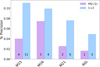 |
Fig. 7 Precision metric (Eq. (6)) of the models in Table 2 for the KiDS sample from the tiles in Table 4. In blue we show the metric computed considering objects with labels 1 and 2 as TPs. In purple, the same metric is shown but for objects with a confidence label of 1. The number at the bottom indicates the total number of TPs found in the ten tiles with each model. |
5.2 Testing of the fine-tuned models on KiDS DR4
Using each dataset specified in Table 3, we individually fine-tuned Model 15 for KiDS. We adhered to the same procedure outlined in Sect. 5.1, randomly selecting ten KiDS tiles. The tile names and characteristics are presented in Table 5 with two of these (KIDS_340.8_-28.2, KIDS_131.0_1.5) situated within the GAMA survey area.
Figure 9 presents the precision achieved on the ten test tiles, for various augmentation techniques. The purple boxes represent the precision for only the HQ candidates, the blue boxes represent the metric for all confirmed candidates and the numbers at the bottom of the boxes the SGL candidates found. Figure 9 demonstrates how the performance of the transformers varies with the fine-tuning dataset. As expected, the model with the most FPs is the one employing the original, not fine-tuned weights – “no fine-tuning”;. The precision of the no fine-tuning model is approximately half of the best-performing fine-tuned model, highlighting the impact of transfer learning. The models with the least FPs are RFT, RF, and R. However, the number of TPs changes substantially between these models. The model fine-tuned with rotated flipped and transposed images, RFT, emerges as the best-performing model in this ten-tile evaluation. The number of FPs significantly impacts the precision of the no fine-tuning model. The model identified 7068 FPs, considerably higher than the 2035 FPs found by the RFT model. While the RF model achieved the lowest number of FPs (1847), it also detected one fewer SGL candidate compared to the RFT model. This tradeoff between FPs and TPs is well depicted by the precision metric.
In total, 23 objects have been labeled as SGL candidates across the ten test tiles, and the ten HQ instances have IDs 5 to 14 in Fig. 10 and Table A.1. The RFT model exhibits an average of 70% fewer FPs than the no fine-tuning model.
6 Application to 221 deg2 of KiDS DR4
The overlapping region between the GAMA and KiDS surveys spans 221 deg2, with the GAMA survey regions’ coordinates provided in Table 1. We employed the RFT model to identify SGLs in this portion of the sky. The preselection yields a target sample of 5 538 525 elements, from which RFT identifies MLcand = 51 626, the full list of these objects with relative KiDS ID, coordinates, label and prediction probability is in Table 6. Throughout this section and the following, we use the term “TEGLIE”; candidates or (TPTEGLIE) to refer to the comprehensive list of all lenses graded 1 or 2. The subset of “HQ TEGLIE”; candidates, denoted by the label 1, encompasses high-confidence SGL candidates.
Upon visual examination, the final list of SGL candidates within the GAMA footprint includes 175 candidates, 56 of which are categorized as HQ SGLs. These HQ candidates, along with those discovered during model testing outside the GAMA region, are combined and presented in Table A.1 and displayed in Fig. 10. Henceforth, we use the indices in the tables to reference specific grade 1 candidates. The merged catalog consists of 264 lens candidates, including 71 HQ candidates. The less certain grade 2 candidates discovered within the GAMA footprint are depicted in the Appendix, illustrated in Fig. C.1 and listed in Table C.1.
To ascertain which of our TEGLIE candidates represent novel discoveries, we cross-checked them against catalogs from other survey searches: KiDS, Survey of gravitationally lensed objects in HSC Imaging (SuGOHI), Pan-STARRS, and Strong Lensing Legacy Survey (SL2S). It is noteworthy that most SGL catalogs published in the literature comprise candidate lenses, with only a small proportion of these having been spectroscopically confirmed so far. Due to the size of our cutouts (20″ × 20″), we cross-matched with other catalogs using a 10″ tolerance. If multiple objects are found, the closest one was considered.
In Table A.1, the “crosscheck”; column indicates the surveys or searches in which these high-confidence candidates were identified. Table 7 presents the number of coinciding elements with the SGL searches that exhibit the highest overlap. The top row lists the names of the various searches, including TEGLIE. HQ KiDS refers to the HQ SGL candidates proposed by the KiDS collaboration in Petrillo et al. (2019) and Li et al. (2020), LinKS encompasses all objects flagged as strong lens candidates by at least one visual inspector Petrillo et al. (2019), and SuG-OHI from Jaelani et al. (2021). Within the SuGOHI survey, we also subdivided the candidates based on their grades: A indicates “definitely a lens”;, B “likely a lens”;, and C “possibly a lens”;. The leftmost column defines the different grade subsets, with 1+2 constituting the sum of candidates with grades 1 and 2.
Of the HQ KiDS SGL candidates, which were incorporated into our fine-tuning set, HQkiDS = 38 fall within this portion of the sky. Of these HQKiDS candidates, ten were not identified by our model: three failed to meet our redshift cutoff, and seven (shown in Fig. 11, image IDs from 5 to 11) did not exceed the prediction probability threshold, even though the model has been trained on these images. Out of the 28 candidates that cleared the prediction probability threshold, 23 have been labeled as TPs, while 5 were deemed FPs. The FP candidates are presented in Fig. 11 (images from 0 to 4). Images 0, 1, and 4 all exhibit an arc-like structure even though the arc in image 1 requires very close inspection to be noticed. These candidates have been overlooked by the visual inspector during the validation process. This demonstrates the challenges of labeling lenses, as both distraction and fatigue can lead to missed candidates. Finally, candidate 3 displays diffuse emission but lacks distinct arcs.
The LinKS dataset comprises TPLinKS = 1983, of which TPLinKS,GAMA = 503 fall within the GAMA survey area. Out of these LinKS candidates, 10 are HQKiDS and of the TPLinKS,GAMA candidates, 354 were also identified by our model (MLcandTEGLIE), and 37 were graded as TPs, including 21 in high-confidence (HQTEGLIE) candidates. Of TPLinKS in HQkiDS 5 have been tagged as FP.
The Hyper Suprime-Cam Subaru Strategic Program (HSC SSP; Miyazaki et al. 2012) has also surveyed this portion of the sky, generating the SuGOHI catalog of 3057 SGL candidates (Sonnenfeld et al. 2017, 2020; Chan et al. 2020; Jaelani et al. 2020; Wong et al. 2022). Among the around 50 000 MLcandTEGLIE candidates identified by our ML model, 194 were found in the SuGOHI catalog. Of these, 37 were confirmed as TPs, and among them, 21 were classified as high-confidence candidates. Notably, 111 of the grade 0 SGLs held a “possibly a lens”; (grade C) classification in SuGOHI. This discrepancy suggests that our grading standards might have been stricter than those used for the HSC lenses. This could be due to factors like different grader expertise or specific selection criteria employed by each project. While most of the higher-grade SuGOHI lenses have been missed by our graders due to the superior resolution and depth of the HSC data.
Furthermore, two candidates have been located and suggested as SGL candidates by the Canada-France-Hawaii Telescope Legacy Survey-Strong legacy survey (SL2S; More et al. 2012). However, only object 21 (SDSSJ1143-0144) has been labeled as HQ TP, while SDSSJ0912+0029, not showing clear lensing structures, has been labeled as a FP.
Three additional lenses (Pan-STARRS ID: PS1J0846-0149, PS1J0921+0214, PS1J1422+0209) in MLcandTEGLIE have been found in the Pan-STARRS candidates sample (Cañameras et al. 2020). However, only PS1J0921+0214 has been labeled a SGL candidate. Upon visual inspection, no clear double images or arc-like structures were found in the images of the missed candidates.
Finally, each candidate in Table A.1 underwent inspection on the SIMBAD astronomical database (Wenger et al. 2000). This check led to the exclusion of one candidate (object 8) due to the lensed object classification as a white dwarf. Candidate 59, is a confirmed strong lens and part of the SDSS Giant Arcs Sample (SGAGS; presented in Hennawi et al. 2008; Bayliss et al. 2011) with ID SGAGS J144133.2-005401 (Rigby et al. 2014). Candidate 38, is a confirmed quadruple-lensed source, initially discovered with the HSC survey (More et al. 2017).
Of the grade 2 objects, 23 have been already located either in SuGOHI or in the KiDS searches.
In summary, our model identified a total of 264 TPTEGLIE, among which 71 HQ candidates with 27 rediscoveries, yielding 44 new HQ candidates discovered exclusively by our model.
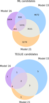 |
Fig. 8 Venn diagram exploring common elements found by different models. Numbers indicate the numbers of elements in common between datasets. Top: diagram of the ML candidates found by the three four-band models. Bottom: diagram of the visually inspected candidates only. |
Ten randomly chosen KiDS tiles used for testing the fine-tuned transformers.
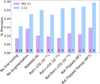 |
Fig. 9 Precision metric (Eq. (6)) for different types of augmented datasets. In blue we show the metric computed considering objects with labels 1 and 2 as TPs. In purple, the same metric is shown but for objects with a confidence label of 1. TP counts are shown at the bottom of every bar. |
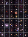 |
Fig. 10 First 48 high-confidence SGL candidates found in this work. The numbers at the top of every cutout correspond to the ID of the object in Table A.1. Images marked with an asterisk are HQ SGL candidates already identified by the KiDS Collaboration. Remaining 23 high-confidence SGL candidates found in this work. |
Catalog of the ML SGL candidates from the 221 deg2 check (extract).
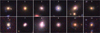 |
Fig. 11 From 0 to 4: SGL candidates found in previous KiDS automated searches (Petrillo et al. 2019; Li et al. 2020) proposed as SGL candidates by our model but rejected by the visual inspectors. From 5 to 11: HQ SGLs found in previous KiDS automated searches not proposed as SGL candidates by our model even though they were in the training set. |
7 Cross-matching with GAMA
The sky region investigated in this study completely overlaps with the GAMA fields, allowing us to search for spectroscopic counterparts. We performed the nearest neighbor matching by right ascension and declination within a 3-arcsecond positional tolerance between the GAMA DR4 catalog and the candidates found in this work. Out of the 264 TEGLIE candidates, we find 144 matches, with 35 of these being high-confidence candidates. Considering that a 3-arcsecond positional tolerance might be too broad for some objects, we implemented an additional verification step. We compared the FLUX_RADIUS values from the SExtractor run of each object in the KiDS catalog. If the separation between the KiDS and GAMA positions is less than the FLUX_RADIUS converted in arcseconds, we considered the crossmatch to be reliable. Twelve sources do not pass this test (eight are grade 2 and four are grade 1).
Using the AATSpecAutozAllv27_DR4 catalog, as detailed in Sect. 3.4, we investigated the TEGLIE candidates spectra. Among the 101 grade 2 candidates with reliable GAMA counterparts, 7 (ID in Table C.1: 9, 60, 111, 112, 150, 153, 186) have either the first or second best-fitting template of a star, while all grade 1 images have galaxy templates. To identify double redshift candidates, we applied the R (Eq. (3)) selection criteria outlined by Holwerda et al. (2015); Knabel et al. (2023) to the grade 1 candidates. With R ≥ 1.85, we found 26 blended spectra. Relaxing the threshold to R ≥ 1.2 increases the number of selected candidates to 31. Among the 31 selected candidates, 13 are ELG+PG, 8 ELG+ELG, 7 PG+ELG, and 3 PG+PG pairs.
We include the spectroscopic redshifts of the first (zspec) and second (zspec,2) correlation peaks of the grade 1 candidates in Table A.1. Figure 12 compares the lens KiDS photometric redshifts with the GAMA spectroscopic redshifts for the “high-confidence”; double redshift candidates (selected with R > 1.2). The error bars represent the minimum and maximum redshift ranges provided in the KiDS catalog. The blue circles represent the “most likely”; redshift derived from spectral fitting for each source. The purple crosses depict an alternative spec-z value, which corresponds to the lower redshift among the two obtained from the two highest correlation peaks identified in the spectra. The figure suggests a possible overestimation of the photo-z values compared to the spec-z, particularly for some sources. This discrepancy could be attributed to the close proximity of the lensing galaxy (central source) to other objects in the field, potentially corresponding to multiple images. Such complex environments can pose challenges for accurate photometric redshift estimation algorithms. Whether this is a systematic effect or specific to our sample requires further investigation.
Holwerda et al. (2015) considered pairs with PGs as the foreground object and ELGs as the background object as potential SGL candidates. Our sample includes seven such PG+ELG configurations, identified with IDs 13, 29, 30, 46, 52, 55 and 67 in Table A.1.
A cross-match (within a 3″ radius) between the Holwerda et al. (2015) sample and the ML candidates (Table 6) revealed 64 overlapping. Among these, 22 have PG+ELG galaxy templates and hence are considered as SGL candidates by Holwerda et al. (2015). Of these 22 double-z SGL candidates, 21 have been labeled as non-lenses during our visual inspection (shown in Fig. E.1) and 1 as grade 3 (ID 20 in Table D.1). Inspecting Fig. E.1, there is no object showing clear lensing features, the objects appear to be serendipitous overlaps of two galaxies rather than gravitationally lensed systems. This highlights the limitations of the blended spectra method for definitive SGL identification. While effective for selecting candidate galaxy pairs, follow-up observations with either high-resolution imaging or further spectroscopical data are crucial for confirmation. This has already been noted by Chan et al. (2016). In their work, only 6 out of 14 PG+ELG candidates from the Holwerda et al. (2015) sample within the HSC field were confirmed as probable lenses, suggesting a success rate of approximately 50% for the blended spectra approach. However, confirmation for the Chan et al. (2016) candidates themselves is still required to solidify this success rate estimate.
Knabel et al. (2020) further refined the selection criteria established by Holwerda et al. (2015) by requiring an absolute difference in the spectroscopic redshifts of the first and second correlation peaks (Δz) to be greater than 0.1. Figure 13 shows the distribution of Δz for PG+ELG pairs (purple) and all other source combinations (blue). As expected, all PG+ELG pairs exhibit Δz > 0.1, making them stronger SGL candidates. The source combinations with Δz < 0.1 include three ELG+PG pairs, three ELG+ELG pairs, and one PG+PG pair.
Knabel et al. (2023) preselected sources with foreground redshifts exceeding 0.05. All configurations in our sample satisfy this criterion except for three ELG+ELG pairs and four ELG+PG pairs, leaving us with 25 potential SGL candidates.
Due to the limited number of source matches between GAMA and KiDS surveys, subsequent sections rely on photometric redshifts for characterizing the properties of the candidates. Additionally, spectroscopic redshifts are unavailable for some of the candidate double redshifts identified in previous studies (Petrillo et al. 2019; Li et al. 2020, 2021). To ensure consistency when comparing our results with these studies, we employ the KiDS photometric redshifts in the following sections.
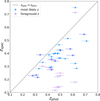 |
Fig. 12 Comparison of the spectroscopic redshifts (zspec) from the GAMA survey with the photometric redshifts (zphot) derived from the nearest neighbor search in KiDS of the 31 grade 1 galaxies with R ≥ 1.2 (Eq. (3)). For objects in GAMA, we utilize the redshift from the AATSpecAutozAllv27_DR4 catalog. The purple crosses represent the KiDS Zphot vs. the lower zspec between the two redshift estimates coming from the two highest correlation peaks from the AUTOZ output. The blue circles illustrate the KiDS zphot vs. the zspec “best-fitting”; redshift (highest cross-correlation) from AUTOZ. The black solid line represents a perfect one-to-one correspondence between the two redshift measurements. |
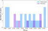 |
Fig. 13 Absolute difference in redshift between the foreground and background galaxies of the 31 grade 1 candidates with a ratio R (Eq. (3)) greater than 1.2. Purple blocks represent the PG + ELG (background + foreground) and blue blocks include all the other galaxy pairs (PG+PG, ELG+ELG, and ELG+PG). |
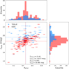 |
Fig. 14 Photometric redshift vs. r-band magnitude space. Red crosses represent lenses found by the KiDS collaboration, with error bars indicating the range between the predicted maximal and minimal estimated redshift given by the BPZ code. Histograms of redshift and magnitude, for both populations, are plotted along each axis to better visualize the distribution of values. Values of the median magnitude and redshift for both samples are represented by dashed lines (TEGLIE), and solid lines (KiDS) and reported in the plot. |
8 Properties of the candidates
In this section, we delve into the characteristics of the 71 HQTEGLIE included in Table A.1, excluding the one classified as a star in the SIMBAD database.
Figure 14 presents photometric redshift versus r-band magnitude and the distribution of two quantities, as in Li et al. (2020), for the HQ SGL candidates identified by KiDS collaboration and in this work. We denote ![Mathematical equation: $\[\tilde{x}\]$](/articles/aa/full_html/2024/08/aa49929-24/aa49929-24-eq14.png) as the median of variable x. The TEGLIE candidates have an r-band magnitude that is slightly fainter than that of the SGL candidates found by the KiDS collaboration, with
as the median of variable x. The TEGLIE candidates have an r-band magnitude that is slightly fainter than that of the SGL candidates found by the KiDS collaboration, with ![Mathematical equation: $\[\widetilde{r}_{\text {TEGLIE }}=19.33\]$](/articles/aa/full_html/2024/08/aa49929-24/aa49929-24-eq15.png) mag compared to
mag compared to ![Mathematical equation: $\[\widetilde{r}_{\mathrm{KiDS}}=18.66\]$](/articles/aa/full_html/2024/08/aa49929-24/aa49929-24-eq16.png) mag. Whereas the redshift median is similar for both datasets,
mag. Whereas the redshift median is similar for both datasets, ![Mathematical equation: $\[\widetilde{z}_{\text {TEGLIE }}=0.46\]$](/articles/aa/full_html/2024/08/aa49929-24/aa49929-24-eq17.png) in this work and
in this work and ![Mathematical equation: $\[\widetilde{z}_{\mathrm{KiDS}}=0.45\]$](/articles/aa/full_html/2024/08/aa49929-24/aa49929-24-eq18.png) for KiDS. This suggests that the TEGLIE candidates are slightly less luminous but share a similar redshift distribution, albeit with a less pronounced peak, to the KiDS sample. Moreover, the redshift distribution of KiDS confirms that selecting a redshift range from 0 to 0.8 was a safe decision, as most of the lenses fall within this range. The lenses identified by KiDS exhibit a correlation between redshift and magnitude, likely attributable to the preselection of BGs. In contrast, the TEGLIE candidates appear more dispersed across the redshift-magnitude space, possibly due to the absence of such a preselection.
for KiDS. This suggests that the TEGLIE candidates are slightly less luminous but share a similar redshift distribution, albeit with a less pronounced peak, to the KiDS sample. Moreover, the redshift distribution of KiDS confirms that selecting a redshift range from 0 to 0.8 was a safe decision, as most of the lenses fall within this range. The lenses identified by KiDS exhibit a correlation between redshift and magnitude, likely attributable to the preselection of BGs. In contrast, the TEGLIE candidates appear more dispersed across the redshift-magnitude space, possibly due to the absence of such a preselection.
In Fig. 15, we present the observer-frame g − r color in relation to the redshift of TEGLIE and KiDS HQ candidates. As mentioned in Sect. 2, the KiDS collaboration preselected a sample of BGs and a subsample of LRGs. This color cut resulted in the selection of KiDS lenses with red colors, g − rKiDS ~0.8 mag at z ~0 and g − rKiDS ~1.6 at z ~0.5. In our case, without any color cut, we still obtain similar results to the KiDS sample. The influence of this color cut is further investigated in a color-color plot in Fig. 16. All sources passing the BG preselection are plotted as red crosses. The LRG selection is determined by an additional magnitude cut and two inequalities as per Eq. (1). The solid pink line represents the boundaries of the lower inequality in Eq. (1), while the pink area indicates the region where the inequality holds. The top inequality in Eq. (1) depends on the r-band magnitude of each object – all candidates satisfying this inequality are plotted as red squares in Fig. 16. As a result, all squares within the pink area of the plot are considered LRGs according to the KiDS formulation. On the other hand, all objects (crosses and squares) outside the pink stripe are thus BGs. Most of the TEGLIE candidates (blue-filled circles) fall within the color cut cperp (pink block) but not all meet the BG preselection criteria. We highlight these “not BG”; candidates with a wider blue circumference. Of the HQ TEGLIE candidates, 57 are BGs based on the criteria outlined in Sec. 2. Specifically, seven candidates have a magnitude greater than 21, and four have SG2DPHOT values equal to 4. These latter candidates (IDs 2, 7, 22, and 58) exhibit a small separation between the two sources and are therefore classified as potential stars, although none of them are tagged as such in SIMBAD.
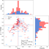 |
Fig. 15 g − r observer-frame color corrected for Galactic extinction vs. photometric redshift. Red crosses represent lenses found by KiDS, with error bars indicating the range between the predicted maximum and minimum estimated redshift. Blue dots represent newly found HQ candidates. Histograms of redshift and color, for both populations, are plotted along each axis to better visualize the distribution of values. Values of the median color and estimated redshift for both populations are represented by dashed lines (TEGLIE) or solid lines (KiDS) and reported in the plot. |
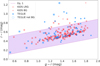 |
Fig. 16 Visualization of the KiDS selection criteria for identifying LRGs and BGs through a color cut, as described in Sec. 2. Our model was applied to a sample without this specific color selection, allowing it to detect candidates that would have otherwise been excluded by the KiDS LRG–BG cut. The blue dots with a circle around are all the TEGLIE HQ (grade 1) candidates that would have been missed with the KiDS preselection. A solid pink line limits the boundaries of the bottom inequality in Eq. (1). The red crosses are the HQ KiDS lenses that satisfy the top inequality in Eq. (1); the red crosses represent all the objects passing the BG selection, as described in Sec. 2. Blue dots are the TEGLIE candidate while the blue circles are all the HQ TEGLIE that would have not been passed the KiDS color cut. |
9 Discussion
9.1 Comparison of model performances
Table 8 summarizes the results of various SGL searches in KiDS, including this work. For this comparison, we considered only the final search on the 221 deg2 overlapping with GAMA. For studies that employ multiple CNN architectures (Petrillo et al. 2019; Li et al. 2021), we report only the three-band (r, i, and g) model results for a more accurate comparison with our four-band TE (r, i, g, and u). Both models leverage color information in addition to morphology, in contrast with the r-band one, which considers only morphology.
The differences in sample sizes between distinct searches – with the same preprocessing (preselection) – are due to differences in sky coverage. The quantity of SGL candidates found by the ML model (ML candidates) instead, is influenced by the prediction probability threshold (p) used to divide the SGL candidates class from the non-lens ones and by the sample size. In the same way, the FPs increase together with the ML candidates and sample size: the more data are provided to the ML model, the more chances of finding FPs. To standardize performance comparison, we calculated the percentage of ML candidates relative to the entire sample (% ML cand), the percentage of FPs within the ML candidates (% FP) long with the precision (P). These metrics provide an overall assessment of model performance.
While expert visual confirmation remains essential for identifying TPs, across studies, significant variations exist in the number of inspectors involved and the grading system employed. This inconsistency can considerably impact the reported percentage of ML candidates. In our work, the majority of visual inspections were conducted by a single author, potentially introducing labeling bias and increasing the risk of overlooking HQ candidates. However, the high false positive rate (FPR) necessitated this approach, as assigning the same lenses to multiple inspectors for confirmation proved impractical and too time-consuming. This highlights the crucial importance of considering these methodological variations when comparing results across different studies.
Table 8 highlights the difference in our model’s precision compared to other SGL searches. While the lower precision in our study could be partially attributed to the sample size investigated, similar-sized samples like in Li et al. (2020) report a significantly higher precision (one order of magnitude greater). This suggests that our model’s performance currently falls short of the competitive level. The primary factor contributing to this discrepancy likely lies in the contrasting training strategies employed. Our model was trained entirely on simulated data before being fine-tuned for the KiDS survey. In contrast, Li et al. (2020) trained their model on real KiDS galaxies with superimposed simulated lensing features. This inherent difference in the training data could explain the observed variation in precision. The next sections will delve deeper into this aspect, exploring the potential influence of training data as well as galaxy population preselection on the model performance.
9.2 Data preselection cuts
Another key difference lies in preprocessing strategies. Early SGL searches (Petrillo et al. 2017, 2018, 2019) targeted only the LRGs subsample, capitalizing on their higher lensing probability (~80%%) compared to the 20% probability of spiral galaxies (see, for instance, Turner et al. 1984). Later studies expanded to include both LRGs and BGs, aiming to generalize the sample beyond a simple color cut. Due to the aforementioned reason, the CNN models in Petrillo et al. (2017, 2018, 2019); Li et al. (2020, 2021) were trained on simulated arcs superimposed on LRGs. This potential bias toward LRGs leads to higher FPs contamination in the BG sample, justifying the higher prediction probability threshold used for this sample in the studies considering this galaxy population.
We considered the impact of different p thresholds and sample selection for the TEGLIE candidates on the GAMA footprint by using preprocessing strategies used in other KiDS SGL searches. Table 8 also shows the outcomes of these selections. This work exhibits a significantly lower precision (around one order of magnitude) than other SGL searches. The BG cut with p > 0.98 yielded improved precision compared to the original redshift cut (z < 0.8), but still remained lower than other studies. Interestingly, the percentage of ML candidates in our work closely aligns with other studies except for the LRG cut, which shows the lowest performance. Furthermore, the TEGLIE candidates with z < 0.8 would have reduced both TPs and FPs by ~20% for BGs and ~70% for LRGs, making the LRG cut overly restrictive. Initially, the ML sample contained 231 candidates with 51 396 FPs (99.55% of all the candidates). Increasing the prediction probability threshold from 0.8 to 0.9 shrunk the ML sample by roughly 37%. Further raising the threshold to 0.98 filtered out an additional ~60%. This stricter threshold also led to a significant reduction in FPs, with a decrease of 40% and 53% for p = 0.9 and p = 0.98, respectively. These findings underline the impact of preselection in the framework of SGL searches.
Table 8 provides insights into both total and high-confidence (grade 1) TPs, with the latter displayed in parentheses within the TP column. Analyzing all TEGLIE candidates reveals a proportional decrease in total TPs as the number of ML candidates shrinks. The LRG cut stands out as an exception, being overly restrictive and leading to a significant reduction in candidates. However, the picture changes when focusing on high-confidence TPs. The LRG cut remains overly restrictive, hindering potential discoveries. The BG cut, instead, maintains most of the confirmed candidates. With p = 0.8 we retain a 94% completeness of the original candidates while achieving a ~20% reduction in FPs. Even more stringent cuts, like p = 0.98, demonstrate significant potential. This cut offers a 61% reduction in FPs while still preserving 68% of the original high-confidence TPs identified with the less restrictive z < 0.8 cut.
9.3 Selecting training data
Another fundamental aspect to consider when comparing ML models is the training set. The TE was trained on the Bologna Lens Challenge dataset outperforming, with a 99% accuracy, all the models that participated in the challenge (Metcalf et al. 2019). The simulated dataset contains 80% fully simulated images and 15% KiDS BG images with added simulated arcs. On the simulated images, KiDS PSF maps of each band were applied. This training set is significantly different from the one used in other SGL searches where the lensed arcs were all superimposed on LRGs images in KiDS. Fine-tuning with real SGL candidates from KiDS improved performance, but not to the level of direct training on KiDS observed galaxies. This suggests that fine-tuning helps mitigate FPs, but it cannot fully compensate for training with images resembling the actual observed data with its specific PSF. This sensibility is known for CNNs but it is valid also for TEs, though the latter should be able to extract and learn the relation between pixels and better understand the morphology of SGLs. Another difference, as evidenced already by Davies et al. (2019) is that the simulated lenses on the Bologna lens challenge had too wide Einstein rings with respect to the ones found in observations.
The presence of FPs is a constant issue in SGL searches. In Table 8 we include the percentage of FPs in respect to the ML candidates and for most of the searches above 90%, with an average of ≈90%. In this work, we explored a way to mitigate the prevalence of FPs generated by ML model when transitioning to a new target set, particularly when moving from simulated data to real observations. SGLs are extremely rare phenomena, making it challenging to assemble a substantial collection of real observations to effectively train ML algorithms for their identification. Due to the scarcity of real SGL observations, simulated images are employed for training ML algorithms. Another reason for the presence of FPs is that real-world observations are inherently more intricate than simulated data, and SGLs may not always exhibit the classic bright arcs paired with a redder central source resulting in more FPs. For instance, training an algorithm to identify arcs in an image does not guarantee a low FPR. Numerous celestial objects possess elongated features that can mimic lensed galaxies, such as the tidal tails of merging galaxies. Additionally, some edge-on galaxies can be misclassified as lensed arcs if they lie in close proximity to another source. Similarly, ring galaxies, which are rare galaxies with a bright ring of stars surrounding a central core, can be confused with Einstein rings (Timmis & Shamir 2017). In this work, we identified 121 objects during visual inspection that exhibited such characteristics and were assigned a grade of 3. These objects are illustrated in Fig. 17.
In Fig. 5, we present some of the non-lenses used in the fine-tuning, these cutouts do not exactly show dubious cases in which a human would have difficulties in the labeling. The discrepancy between human and machine perception of relevant features emphasizes the importance of having a diverse dataset, including images similar to lenses. While incorporating genuine SGL images is essential for training models, it is equally important to include misleading objects for both human experts and ML models. Figure 17 exemplifies such cases. Certain features like elongation and the presence of brighter arcs or redder central sources are not conclusive indicators of SGLs, as the presence of multiple objects with similar colors can lead to ambiguity, making visual inspection challenging even for experienced inspectors, as discussed in Rojas et al. (2023).
As previously discussed in Rojas et al. (2022), a dataset that includes ring galaxies and other potential FPs will be valuable for training more accurate models in the future. Datasets with misleading objects are important for training ML algorithms; however, as discussed in Wilde et al. (2022), this approach has a fundamental interpretability problem. It is not possible to directly understand how the model works, which features of SGLs the model learns, or if there is a substantial bias toward a class of lenses. The “black-box”; issue is a critical problem in ML studies and understanding the biases of these algorithms is vital (e.g., Obermeyer et al. 2019; Yip et al. 2021; Chou et al. 2022; Chen et al. 2023; Ferrara 2024). Machine learning methods excel at modeling high-dimensional data by capturing intricate nonlinear relationships. Consequently, handling models with billions of parameters is a challenging endeavor.
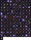 |
Fig. 17 Grade 3 objects, mostly mergers and ring galaxies. |
9.4 Model interpretability and biases
Several techniques, such as GradCAM (Selvaraju et al. 2019) and LIME (Ribeiro et al. 2016), can be employed to pinpoint the features that play a crucial role in a model’s decision-making process. However, these methods are not suitable for the present scenario due to their constraints. GradCAM is only applicable to CNNs, while LIME is incapable of handling images with more than three dimensions, making it unsuitable for the four-band image data used to train the model. Techniques like GradCAM and other input-altering approaches, such as masking specific regions of the image, have been investigated in Wilde et al. (2022) to enhance the interpretability of CNNs for SGL detection. These methods suggest that models tend to prioritize lenses exhibiting blue ring-like features. However, observations of Einstein rings and lensed dusty forming galaxies have been reported in the literature (Negrello et al. 2010, 2016; Geach et al. 2015; Spilker et al. 2016; Rivera et al. 2019; Neri et al. 2020), highlighting a potential limitation of ML models for SGL detection if they rely heavily on the lensing systems’ colors.
One approach to mitigating bias in ML classifications could involve ensembling different architectures with varying hyperparameters, trained on diverse datasets. The final label could then be determined by averaging the prediction probabilities of these individual networks, as demonstrated by Canameras et al. (2023) and Schaefer et al. (2018). Alternatively, a more structured approach could involve incorporating the calibrated probabilities generated within a Bayesian framework, as presented in Holloway et al. (2024). Averaging the predictions of multiple models can lead to a more robust detection algorithm. This, combined with enhanced training data and the contributions of citizen science initiatives, holds the potential to drive significant scientific advancements in the years to come.
For next-generation surveys like the LSST, a combination of methods and ML models will be essential. This process could begin with a robust preselection step to identify galaxies with a statistically high likelihood of being strong lenses. Subsequently, a variety of ML models and algorithms could be employed for precise feature detection and FP reduction. Finally, by combining ML with citizen science initiatives like the Space Warps project (Marshall et al. 2016), the accurate labeling of all SGL candidates could be achieved.
10 Conclusions
This paper presents a methodology for mitigating the challenge of FPs arising from ML models employed for SGL detection. Our approach incorporates images of real SGL candidates and non-SGL examples alongside data augmentation techniques. Utilizing this augmented dataset, we fine-tuned a pretrained model, originally developed using simulated data that approximate the KiDS observations, to enhance its performance on real KiDS data. Through an evaluation of six different data augmentation techniques, we identified the combination of rotation, flipping, and transposed image augmentation as the most effective, achieving a 70% reduction in FPs.
Applying our method to a 221 deg2 region co-observed by the KiDS and GAMA surveys yielded 56 high-confidence and 175 less certain SGL candidate detections. These candidates originated from a relaxed galaxy selection compared to previous searches, incorporating all galaxies up to redshift 0.8. Incorporating the SGL candidates identified during the testing phase of the fine-tuned model, the total number of HQ SGL candidates increases to 71. Of these 71, 44 candidates are entirely new detections, not previously identified by other methods.
Our analysis reveals that stricter selection criteria would have significantly reduced the number of candidates. Focusing solely on BGs would have decreased both TPs (grade 1 and 2) and FPs by 20%. Further restricting ourselves to the LRG population would have reduced both categories by 70%, hindering discoveries. However, with the BG cut and considering only high-confidence candidates, we would have retrieved 94% of them while still achieving a 20% reduction in FPs.
Among the high-confidence SGLs, 31 pass the double-redshift selection using the GAMA survey data. Of these, seven show blended spectra of PGs in the foreground as ELGs in the background, confirming their chance of being strong lenses and enabling further analysis for lens modeling and property investigation in future work.
Additionally, we provide a catalog of 121 FPs that exhibit features resembling those of SGLs, such as bright arcs, bent structures, and ring galaxies. This catalog provides valuable training data for future ML models, aiding in their ability to differentiate true SGLs and further minimize FP detections.
Our work highlights the efficacy of fine-tuning with data augmentation in enhancing the performance of ML models for SGL detection. The fine-tuned model achieved a significant reduction in FPs, detecting 70% fewer compared to the non-fine-tuned model. We also demonstrate the importance of the selection cuts in galaxy populations, which enables the identification of novel SGL candidates while simultaneously reducing the number of FPs. However, our model has still not reached competitive performance. While the model architecture demonstrates strong performance on simulated data (as reported by Thuruthipilly et al. 2022), the current limitation suggests the need for more realistic simulations of SGL systems during the training phase. Incorporating such data has the potential to significantly enhance the model’s ability to detect real-world SGLs. Furthermore, a multifaceted approach – including fine-tuning, citizen science efforts, and model ensembles – is likely the most effective strategy for minimizing FPs. Citizen science can play a crucial role in scrutinizing all the SGL candidates identified by ML models. Looking ahead, the adoption of novel architectures like TEs and widely used models like CNNs holds promise for furthering the field of strong lens identification in wide-area surveys such as LSST.
Acknowledgements
The authors wish to express their gratitude to Alessandro Sonnenfeld for the enlightening discussion, to Junais for the useful comments, and to Shuaibo Geng for helping with the visual inspection. This research was supported by the Polish National Science Centre grant UMO-2018/30/M/ST9/00757 and by Polish Ministry of Science and Higher Education grant DIR/WK/2018/12. This article/publication is based upon work from COST Action CA21136 – “Addressing observational tensions in cosmology with systematics and fundamental physics (CosmoVerse)”;, supported by COST (European Cooperation in Science and Technology). M.L. and V.E. acknowledge support from the South African Radio Astronomy Observatory and the National Research Foundation (NRF) towards this research. Opinions expressed and conclusions arrived at, are those of the authors and are not necessarily to be attributed to the NRF. Based on observations made with ESO Telescopes at the La Silla Paranal Observatory under programme IDs 177.A-3016, 177.A-3017, 177.A-3018 and 179.A-2004, and on data products produced by the KiDS consortium. The KiDS production team acknowledges support from: Deutsche Forschungsgemeinschaft, ERC, NOVA and NWO-M grants; Target; the University of Padova, and the University Federico II (Naples). GAMA is a joint European-Australasian project based around a spectroscopic campaign using the Anglo-Australian Telescope. The GAMA input catalogue is based on data taken from the Sloan Digital Sky Survey and the UKIRT Infrared Deep Sky Survey. Complementary imaging of the GAMA regions is being obtained by a number of independent survey programmes including GALEX MIS, VST KiDS, VISTA VIKING, WISE, Herschel-ATLAS, GMRT and ASKAP providing UV to radio coverage. GAMA is funded by the STFC (UK), the ARC (Australia), the AAO, and the participating institutions. The GAMA website is https://www.gama-survey.org/.
Appendix A Grade 1 candidates
High-quality candidates identified through visual inspection.
Appendix B Metrics for labeled dataset
Metrics are necessary to evaluate the effectiveness of ML models. In our case, metrics provide a quantitative measure of a model’s ability to distinguish between lenses and non-lenses. The number of TPs and true negatives (TNs), representing correctly classified images, and the number of FPs and false negatives (FNs), representing misclassified images, are ideal metrics but often unavailable for real-world datasets due to the difficulty of obtaining labeled data. In the Bologna Lens Challenge, where labels were readily available, the models were evaluated using the area under the receiver operating characteristic curve (AUROC) and true positive rate (TPR).
The receiver operating characteristic (ROC) curve is constructed by plotting the TPR against the FPR at different thresholds. The area enclosed by this curve represents the AUROC value. A perfect model would have an AUROC of 1.0, while a completely random model would have an AUROC of 0.5.
TPR, also called sensitivity, is defined as
![Mathematical equation: $\[T P R=\frac{T P}{T P+F N},\]$](/articles/aa/full_html/2024/08/aa49929-24/aa49929-24-eq19.png) (B.1)
(B.1)
and the FPR as
![Mathematical equation: $\[F P R=\frac{F P}{F P+T N}.\]$](/articles/aa/full_html/2024/08/aa49929-24/aa49929-24-eq20.png) (B.2)
(B.2)
Appendix C Grade 2 candidates
Candidates identified through visual inspection with grade 2.
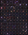 |
Fig. C.1 TEGLIE grade 2 objects. These candidates exhibit some lensing features such as a distorted arc or multiple images. However, these features are not definitive enough to confirm the lensing hypothesis. The images marked with an asterisk are HQ lens candidates already identified by the KiDS collaboration. |
Appendix D Grade 3 candidates
Grade 3 candidates found during the search within the GAMA footprint.
Appendix E Blended spectra search
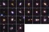 |
Fig. E.1 Strong lens candidates found through the blended spectra search by Holwerda et al. (2015) and labeled as not lenses during the visual inspection. |
References
- Allam, T. J., & McEwen, J. D. 2023, RAS Tech. Instrum., 3, 209 [Google Scholar]
- Aslahishahri, M., Ubbens, J., & Stavness, I. 2023, arXiv e-prints [arXiv:2307.08837] [Google Scholar]
- Baldry, I. K., Alpaslan, M., Bauer, A. E., et al. 2014, MNRAS, 441, 2440 [Google Scholar]
- Barnabè, M., Dutton, A. A., Marshall, P. J., et al. 2012, MNRAS, 423, 1073 [Google Scholar]
- Bayliss, M. B., Gladders, M. D., Oguri, M., et al. 2011, ApJ, 727, L26 [NASA ADS] [CrossRef] [Google Scholar]
- Benítez, N. 2011, Astrophysics Source Code Library [record ascl:1108.011] [Google Scholar]
- Bertin, E., & Arnouts, S. 1996, A&AS, 117, 393 [NASA ADS] [CrossRef] [EDP Sciences] [Google Scholar]
- Bolton, A. S., Burles, S., Koopmans, L. V. E., et al. 2008, ApJ, 682, 964 [Google Scholar]
- Boylan-Kolchin, M., Springel, V., White, S. D. M., Jenkins, A., & Lemson, G. 2009, MNRAS, 398, 1150 [Google Scholar]
- Brownstein, J. R., Bolton, A. S., Schlegel, D. J., et al. 2011, ApJ, 744, 41 [Google Scholar]
- Cañameras, R., Schuldt, S., Suyu, S. H., et al. 2020, A&A, 644, A163 [Google Scholar]
- Canameras, R., Schuldt, S., Shu, Y., et al. 2021, A&A, 653, L6 [NASA ADS] [CrossRef] [EDP Sciences] [Google Scholar]
- Canameras, R., Schuldt, S., Shu, Y., et al. 2023, arXiv e-prints [arXiv:2306.03136] [Google Scholar]
- Cao, S., Biesiada, M., Gavazzi, R., Piórkowska, A., & Zhu, Z.-H. 2015, ApJ, 806, 185 [NASA ADS] [CrossRef] [Google Scholar]
- Cao, S., Li, X., Biesiada, M., et al. 2017, ApJ, 835, 92 [NASA ADS] [CrossRef] [Google Scholar]
- Capaccioli, M., & Schipani, P. 2011, The Messenger, 146, 27 [NASA ADS] [Google Scholar]
- Carion, N., Massa, F., Synnaeve, G., et al. 2020, in Computer Vision – ECCV 2020, eds. A. Vedaldi, H. Bischof, T. Brox, & J.-M. Frahm (Cham: Springer International Publishing), 213 [Google Scholar]
- Chan, J. H. H., Suyu, S. H., More, A., et al. 2016, ApJ, 832, 135 [NASA ADS] [CrossRef] [Google Scholar]
- Chan, J. H. H., Suyu, S. H., Sonnenfeld, A., et al. 2020, A&A, 636, A87 [NASA ADS] [CrossRef] [EDP Sciences] [Google Scholar]
- Chen, P., Wu, L., & Wang, L. 2023, Appl. Sci., 13, 10258 [CrossRef] [Google Scholar]
- Chou, Y.-L., Moreira, C., Bruza, P., Ouyang, C., & Jorge, J. 2022, Inf. Fusion, 81, 59 [CrossRef] [Google Scholar]
- Collett, T. E. 2015, ApJ, 811, 20 [NASA ADS] [CrossRef] [Google Scholar]
- Collett, T. E., & Auger, M. W. 2014, MNRAS, 443, 969 [NASA ADS] [CrossRef] [Google Scholar]
- Davies, A., Serjeant, S., & Bromley, J. M. 2019, MNRAS, 487, 5263 [NASA ADS] [CrossRef] [Google Scholar]
- de Jong, J. T. A., Verdoes Kleijn, G. A., Kuijken, K. H., & Valentijn, E. A. 2013, Exp. Astron., 35, 25 [Google Scholar]
- de Jong, J. T. A., Verdoes Kleijn, G. A., Boxhoorn, D. R., et al. 2015, A&A, 582, A62 [NASA ADS] [CrossRef] [EDP Sciences] [Google Scholar]
- de Jong, J. T. A., Verdoes Kleijn, G. A., Erben, T., et al. 2017, A&A, 604, A134 [NASA ADS] [CrossRef] [EDP Sciences] [Google Scholar]
- Devlin, J., Chang, M.-W., Lee, K., & Toutanova, K. 2019, arXiv e-prints [arXiv:1810.04805] [Google Scholar]
- Diehl, H. T., Buckley-Geer, E. J., Lindgren, K. A., et al. 2017, ApJS, 232, 15 [NASA ADS] [CrossRef] [Google Scholar]
- Donoso-Oliva, C., Becker, I., Protopapas, P., et al. 2023, A&A, 670, A54 [NASA ADS] [CrossRef] [EDP Sciences] [Google Scholar]
- Dosovitskiy, A., Beyer, L., Kolesnikov, A., et al. 2021, in 9th International Conference on Learning Representations, ICLR 2021, Virtual Event, Austria, May 3–7, 2021 (OpenReview.net) [Google Scholar]
- Driver, S. P., Norberg, P., Baldry, I. K., et al. 2009, Astron. Geophys., 50, 5.12 [NASA ADS] [CrossRef] [Google Scholar]
- Driver, S. P., Hill, D. T., Kelvin, L. S., et al. 2011, MNRAS, 413, 971 [Google Scholar]
- Driver, S. P., Bellstedt, S., Robotham, A. S. G., et al. 2022, MNRAS, 513, 439 [NASA ADS] [CrossRef] [Google Scholar]
- Dye, S., & Warren, S. J. 2005, ApJ, 623, 31 [NASA ADS] [CrossRef] [Google Scholar]
- Eisenstein, D. J., Annis, J., Gunn, J. E., et al. 2001, AJ, 122, 2267 [Google Scholar]
- Faure, C., Kneib, J.-P., Covone, G., et al. 2008, ApJS, 176, 19 [NASA ADS] [CrossRef] [Google Scholar]
- Ferrara, E. 2024, Science, 6 [Google Scholar]
- Garvin, E. O., Kruk, S., Cornen, C., et al. 2022, A&A, 667, A141 [NASA ADS] [CrossRef] [EDP Sciences] [Google Scholar]
- Geach, J. E., More, A., Verma, A., et al. 2015, MNRAS, 452, 502 [NASA ADS] [CrossRef] [Google Scholar]
- Gentile, F., Tortora, C., Covone, G., et al. 2021, MNRAS, 510, 500 [NASA ADS] [CrossRef] [Google Scholar]
- He, K., Zhang, X., Ren, S., & Sun, J. 2016, in 2016 IEEE Conference on Computer Vision and Pattern Recognition (CVPR), 770 [Google Scholar]
- He, Z., Er, X., Long, Q., et al. 2020, MNRAS, 497, 556 [NASA ADS] [CrossRef] [Google Scholar]
- Hennawi, J. F., Gladders, M. D., Oguri, M., et al. 2008, AJ, 135, 664 [NASA ADS] [CrossRef] [Google Scholar]
- Hezaveh, Y., Dalal, N., Holder, G., et al. 2016, J. Cosmol. Astropart. Phys., 2016, 048 [CrossRef] [Google Scholar]
- Holloway, P., Marshall, P. J., Verma, A., et al. 2024, MNRAS, 530, 1297 [NASA ADS] [CrossRef] [Google Scholar]
- Holwerda, B. W., Baldry, I. K., Alpaslan, M., et al. 2015, MNRAS, 449, 4277 [NASA ADS] [CrossRef] [Google Scholar]
- Huang, G., Liu, Z., Van Der Maaten, L., & Weinberger, K. Q. 2017, 2261 [Google Scholar]
- Huang, X., Storfer, C., Ravi, V., et al. 2020, ApJ, 894, 78 [NASA ADS] [CrossRef] [Google Scholar]
- Huang, X., Storfer, C., Gu, A., et al. 2021, ApJ, 909, 27 [NASA ADS] [CrossRef] [Google Scholar]
- Huang, K.-W., Chih-Fan Chen, G., Chang, P.-W., et al. 2022, arXiv e-prints [arXiv:2210.04143] [Google Scholar]
- Hwang, S. Y., Sabiu, C. G., Park, I., & Hong, S. E. 2023, J. Cosmol. Astropart. Phys., 2023, 075 [CrossRef] [Google Scholar]
- Jacobs, C., Collett, T., Glazebrook, K., et al. 2019, ApJS, 243, 17 [Google Scholar]
- Jaelani, A. T., More, A., Oguri, M., et al. 2020, MNRAS, 495, 1291 [Google Scholar]
- Jaelani, A. T., Rusu, C. E., Kayo, I., et al. 2021, MNRAS, 502, 1487 [NASA ADS] [CrossRef] [Google Scholar]
- Jia, P., Sun, R., Li, N., et al. 2023, AJ, 165, 26 [NASA ADS] [CrossRef] [Google Scholar]
- Khan, S., Naseer, M., Hayat, M., et al. 2022, ACM Comput. Surv., 54, 1 [CrossRef] [Google Scholar]
- Knabel, S., Steele, R. L., Holwerda, B. W., et al. 2020, AJ, 160, 223 [NASA ADS] [CrossRef] [Google Scholar]
- Knabel, S., Holwerda, B. W., Nightingale, J., et al. 2023, MNRAS, 520, 804 [NASA ADS] [CrossRef] [Google Scholar]
- Krizhevsky, A., Sutskever, I., & Hinton, G. E. 2012, in Advances in Neural Information Processing Systems, 25, eds. F. Pereira, C. Burges, L. Bottou, & K. Weinberger (Curran Associates, Inc.) [Google Scholar]
- Kuijken, K. 2008, A&A, 482, 1053 [NASA ADS] [CrossRef] [EDP Sciences] [Google Scholar]
- Kuijken, K. 2011, The Messenger, 146, 8 [NASA ADS] [Google Scholar]
- Kuijken, K., Heymans, C., Dvornik, A., et al. 2019, A&A, 625, A2 [NASA ADS] [CrossRef] [EDP Sciences] [Google Scholar]
- La Barbera, F., de Carvalho, R. R., Kohl-Moreira, J. L., et al. 2008, PASP, 120, 681 [NASA ADS] [CrossRef] [Google Scholar]
- Laureijs, R., Amiaux, J., Arduini, S., et al. 2011, arXiv e-prints [arXiv:1110.3193] [Google Scholar]
- LeCun, Y., Bottou, L., Bengio, Y., & Haffner, P. 1998, Proc. IEEE, 86, 2278 [Google Scholar]
- Lewis, D. D., & Gale, W. A. 1994, 3 [Google Scholar]
- Li, R., Napolitano, N. R., Tortora, C., et al. 2020, ApJ, 899, 30 [Google Scholar]
- Li, R., Napolitano, N. R., Spiniello, C., et al. 2021, ApJ, 923, 16 [NASA ADS] [CrossRef] [Google Scholar]
- Li, X., Ding, H., Yuan, H., et al. 2023, arXiv e-prints [arXiv:2304.09854] [Google Scholar]
- Liske, J., Baldry, I. K., Driver, S. P., et al. 2015, MNRAS, 452, 2087 [Google Scholar]
- LSST Science Collaboration (Abell, P. A., et al.) 2009, arXiv e-prints [arXiv:0912.0201] [Google Scholar]
- Lupton, R., Blanton, M. R., Fekete, G., et al. 2004, PASP, 116, 133 [NASA ADS] [CrossRef] [Google Scholar]
- Marshall, P. J., Verma, A., More, A., et al. 2016, MNRAS, 455, 1171 [NASA ADS] [CrossRef] [Google Scholar]
- Merz, G., Liu, Y., Burke, C. J., et al. 2023, MNRAS, 526, 1122 [NASA ADS] [CrossRef] [Google Scholar]
- Metcalf, R. B., & Petkova, M. 2014, MNRAS, 445, 1942 [NASA ADS] [CrossRef] [Google Scholar]
- Metcalf, R. B., Meneghetti, M., Avestruz, C., et al. 2019, A&A, 625, A119 [NASA ADS] [CrossRef] [EDP Sciences] [Google Scholar]
- Miyazaki, S., Komiyama, Y., Nakaya, H., et al. 2012, SPIE Conf. Ser., 8446, 84460Z [NASA ADS] [Google Scholar]
- More, A., Cabanac, R., More, S., et al. 2012, ApJ, 749, 38 [NASA ADS] [CrossRef] [Google Scholar]
- More, A., Verma, A., Marshall, P. J., et al. 2015, MNRAS, 455, 1191 [Google Scholar]
- More, A., Lee, C.-H., Oguri, M., et al. 2017, MNRAS, 465, 2411 [NASA ADS] [CrossRef] [Google Scholar]
- Mumuni, A., & Mumuni, F. 2022, Array, 16, 100258 [CrossRef] [Google Scholar]
- Negrello, M., Hopwood, R., Zotti, G. D., et al. 2010, Science, 330, 800 [NASA ADS] [CrossRef] [Google Scholar]
- Negrello, M., Amber, S., Amvrosiadis, A., et al. 2016, MNRAS, 465, 3558 [Google Scholar]
- Neri, R., Cox, P., Omont, A., et al. 2020, A&A, 635, A7 [NASA ADS] [CrossRef] [EDP Sciences] [Google Scholar]
- Nightingale, J. W., Massey, R. J., Harvey, D. R., et al. 2019, MNRAS, 489, 2049 [NASA ADS] [Google Scholar]
- Obermeyer, Z., Powers, B., Vogeli, C., & Mullainathan, S. 2019, Science, 366, 447 [CrossRef] [PubMed] [Google Scholar]
- O’Donnell, J. H., Wilkinson, R. D., Diehl, H. T., et al. 2022, ApJS, 259, 27 [CrossRef] [Google Scholar]
- Oguri, M., & Marshall, P. J. 2010, MNRAS, 405, 2579 [NASA ADS] [Google Scholar]
- Pan, S. J., & Yang, Q. 2010, IEEE Trans. Knowl. Data Eng., 22, 1345 [Google Scholar]
- Paul, S., & Chen, P.-Y. 2022, Proc. AAAI Conf. Artif. Intell., 36, 2071 [Google Scholar]
- Petkova, M., Metcalf, R. B., & Giocoli, C. 2014, MNRAS, 445, 1954 [NASA ADS] [CrossRef] [Google Scholar]
- Petrillo, C. E., Tortora, C., Chatterjee, S., et al. 2017, MNRAS, 472, 1129 [Google Scholar]
- Petrillo, C. E., Tortora, C., Chatterjee, S., et al. 2018, MNRAS, 482, 807 [NASA ADS] [Google Scholar]
- Petrillo, C. E., Tortora, C., Vernardos, G., et al. 2019, MNRAS, 484, 3879 [Google Scholar]
- Rezaei, S., McKean, J. P., Biehl, M., de Roo, W., & Lafontaine, A. 2022, MNRAS, 517, 1156 [NASA ADS] [CrossRef] [Google Scholar]
- Ribeiro, M. T., Singh, S., & Guestrin, C. 2016, arXiv e-prints [arXiv:1602.04938] [Google Scholar]
- Rigby, J. R., Bayliss, M. B., Gladders, M. D., et al. 2014, ApJ, 790, 44 [NASA ADS] [CrossRef] [Google Scholar]
- Rivera, J., Baker, A. J., Gallardo, P. A., et al. 2019, ApJ, 879, 95 [NASA ADS] [CrossRef] [Google Scholar]
- Rojas, K., Savary, E., Clément, B., et al. 2022, A&A, 668, A73 [NASA ADS] [CrossRef] [EDP Sciences] [Google Scholar]
- Rojas, K., Collett, T. E., Ballard, D., et al. 2023, MNRAS, 523, 4413 [NASA ADS] [CrossRef] [Google Scholar]
- Schaefer, C., Geiger, M., Kuntzer, T., & Kneib, J.-P. 2018, A&A, 611, A2 [NASA ADS] [CrossRef] [EDP Sciences] [Google Scholar]
- Schneider, P., Ehlers, J., & Falco, E. E. 1992 [Google Scholar]
- Seidel, G., & Bartelmann, M. 2007, A&A, 472, 341 [NASA ADS] [CrossRef] [EDP Sciences] [Google Scholar]
- Selvaraju, R. R., Cogswell, M., Das, A., et al. 2019, Int. J. Comput. Vis., 128, 336 [Google Scholar]
- Shu, Y., Brownstein, J. R., Bolton, A. S., et al. 2017, ApJ, 851, 48 [Google Scholar]
- Shu, Y., Cañameras, R., Schuldt, S., et al. 2022, A&A, 662, A4 [NASA ADS] [CrossRef] [EDP Sciences] [Google Scholar]
- Simonyan, K., & Zisserman, A. 2015, arXiv e-prints [arXiv:1409.1556] [Google Scholar]
- Sonnenfeld, A., Chan, J. H. H., Shu, Y., et al. 2017, PASJ, 70 [Google Scholar]
- Sonnenfeld, A., Verma, A., More, A., et al. 2020, A&A, 642, A148 [NASA ADS] [CrossRef] [EDP Sciences] [Google Scholar]
- Spilker, J. S., Marrone, D. P., Aravena, M., et al. 2016, ApJ, 826, 112 [NASA ADS] [CrossRef] [Google Scholar]
- Stein, G., Blaum, J., Harrington, P., Medan, T., & Lukić, Z. 2022, ApJ, 932, 107 [NASA ADS] [CrossRef] [Google Scholar]
- Storfer, C., Huang, X., Gu, A., et al. 2022, arXiv e-prints [arXiv:2206.02764] [Google Scholar]
- Szegedy, C., Liu, W., Jia, Y., et al. 2015, in 2015 IEEE Conference on Computer Vision and Pattern Recognition (CVPR), 1 [Google Scholar]
- Tan, M., & Le, Q. 2019, International Conference on Machine Learning, 6105 [Google Scholar]
- Thuruthipilly, H., Zadrozny, A., Pollo, A., & Biesiada, M. 2022, A&A, 664, A4 [NASA ADS] [CrossRef] [EDP Sciences] [Google Scholar]
- Thuruthipilly, H., Grespan, M., & Zadrożny, A. 2024a, AIP Conf. Proc., 3061, 040003 [NASA ADS] [CrossRef] [Google Scholar]
- Thuruthipilly, H., Junais, Pollo, A., et al. 2024b, A&A, 682, A4 [NASA ADS] [CrossRef] [EDP Sciences] [Google Scholar]
- Timmis, I., & Shamir, L. 2017, ApJS, 231, 2 [NASA ADS] [CrossRef] [Google Scholar]
- Tran, K.-V. H., Harshan, A., Glazebrook, K., et al. 2022, AJ, 164, 148 [NASA ADS] [CrossRef] [Google Scholar]
- Turner, E. L., Ostriker, J. P., & Gott, J. R. I., 1984, ApJ, 284, 1 [NASA ADS] [CrossRef] [Google Scholar]
- Vaswani, A., Shazeer, N., Parmar, N., et al. 2017, in Advances in Neural Information Processing Systems 30: Annual Conference on Neural Information Processing Systems 2017, December 4–9, 2017, Long Beach, CA, USA, 5998 [Google Scholar]
- Verma, A., Collett, T., Smith, G. P., Strong Lensing Science Collaboration, & the DESC Strong Lensing Science Working Group. 2019 arXiv e-prints [arXiv:1902.05141] [Google Scholar]
- Wang, Z., Ng, P., Ma, X., Nallapati, R., & Xiang, B. 2019, Assoc. Computat. Linguist., 5878 [Google Scholar]
- Wei, J.-J., Chen, Y., Cao, S., & Wu, X.-F. 2022, ApJ, 927, L1 [NASA ADS] [CrossRef] [Google Scholar]
- Wenger, M., Ochsenbein, F., Egret, D., et al. 2000, A&ASS, 143, 9 [NASA ADS] [CrossRef] [EDP Sciences] [Google Scholar]
- Wilde, J., Serjeant, S., Bromley, J. M., et al. 2022, MNRAS, 512, 3464 [Google Scholar]
- Wong, K. C., Chan, J. H. H., Chao, D. C.-Y., et al. 2022, PASJ, 74, 1209 [CrossRef] [Google Scholar]
- Wortsman, M., Ilharco, G., Gadre, S. Y., et al. 2022, PMLR, 162, 23965 [Google Scholar]
- Xu, M., Yoon, S., Fuentes, A., & Park, D. S. 2023, Pattern Recognit., 137, 109347 [NASA ADS] [CrossRef] [Google Scholar]
- Yip, K. H., Changeat, Q., Nikolaou, N., et al. 2021, AJ, 162, 195 [NASA ADS] [CrossRef] [Google Scholar]
- Yosinski, J., Clune, J., Bengio, Y., & Lipson, H. 2014, in Advances in Neural Information Processing Systems, 27, eds. Z. Ghahramani, M. Welling, C. Cortes, N. Lawrence, & K. Weinberger (Curran Associates, Inc.) [Google Scholar]
- Yu, J., Wang, Z., Vasudevan, V., et al. 2022, Trans. Mach. Learn. Res., 2022 [Google Scholar]
- Zaborowski, E. A., Drlica-Wagner, A., Ashmead, F., et al. 2023, ApJ, 954, 68 [NASA ADS] [CrossRef] [Google Scholar]
All Tables
Name, model structure, AUROC, TPR, and FPR of the models from Thuruthipilly et al. (2022) used in this study.
Ten randomly chosen KiDS tiles used for testing the transformers on the survey data.
All Figures
|
Fig. 1 Schematic view of this work’s methodology. The eye icon denotes the process of visually evaluating ML candidates, and T+22 stands for Thuruthipilly et al. (2022). The comprehensive details of each step in this flowchart are presented in Sec. 4. |
| In the text | |
|
Fig. 2 Scheme of the general architecture of the TE. The extracted features of the input image by the CNN backbone are combined with positional encoding and passed on to the encoder layer to assign attention scores to each feature. The weighted features are then passed to the feed-forward neural network to predict the probability. |
| In the text | |
|
Fig. 3 Selection of the exemplary strong lens candidates found by the KiDS collaboration in DR4 (Li et al. 2020; Petrillo et al. 2019) and implemented in the fine-tuning dataset. |
| In the text | |
|
Fig. 4 High-quality KiDS SGL candidate (ICRS coordinates J030540.105-293416) cutout with different data augmentations. |
| In the text | |
|
Fig. 5 Examples of cutouts employed as non-lenses in the fine-tuning dataset. |
| In the text | |
|
Fig. 6 Prediction probability sample extracted from the ten tiles in Table 4. Left: prediction probability of the four models used in this work from Thuruthipilly et al. (2022). The black line shows the threshold probability; every object above 0.8 is considered an ML candidate. Right: total number of ML candidates compared to the TPs with grades 1 and 2 (TEGLIE candidates) for every model. Bar element counts are shown above each bar. |
| In the text | |
|
Fig. 7 Precision metric (Eq. (6)) of the models in Table 2 for the KiDS sample from the tiles in Table 4. In blue we show the metric computed considering objects with labels 1 and 2 as TPs. In purple, the same metric is shown but for objects with a confidence label of 1. The number at the bottom indicates the total number of TPs found in the ten tiles with each model. |
| In the text | |
|
Fig. 8 Venn diagram exploring common elements found by different models. Numbers indicate the numbers of elements in common between datasets. Top: diagram of the ML candidates found by the three four-band models. Bottom: diagram of the visually inspected candidates only. |
| In the text | |
|
Fig. 9 Precision metric (Eq. (6)) for different types of augmented datasets. In blue we show the metric computed considering objects with labels 1 and 2 as TPs. In purple, the same metric is shown but for objects with a confidence label of 1. TP counts are shown at the bottom of every bar. |
| In the text | |
|
Fig. 10 First 48 high-confidence SGL candidates found in this work. The numbers at the top of every cutout correspond to the ID of the object in Table A.1. Images marked with an asterisk are HQ SGL candidates already identified by the KiDS Collaboration. Remaining 23 high-confidence SGL candidates found in this work. |
| In the text | |
|
Fig. 11 From 0 to 4: SGL candidates found in previous KiDS automated searches (Petrillo et al. 2019; Li et al. 2020) proposed as SGL candidates by our model but rejected by the visual inspectors. From 5 to 11: HQ SGLs found in previous KiDS automated searches not proposed as SGL candidates by our model even though they were in the training set. |
| In the text | |
|
Fig. 12 Comparison of the spectroscopic redshifts (zspec) from the GAMA survey with the photometric redshifts (zphot) derived from the nearest neighbor search in KiDS of the 31 grade 1 galaxies with R ≥ 1.2 (Eq. (3)). For objects in GAMA, we utilize the redshift from the AATSpecAutozAllv27_DR4 catalog. The purple crosses represent the KiDS Zphot vs. the lower zspec between the two redshift estimates coming from the two highest correlation peaks from the AUTOZ output. The blue circles illustrate the KiDS zphot vs. the zspec “best-fitting”; redshift (highest cross-correlation) from AUTOZ. The black solid line represents a perfect one-to-one correspondence between the two redshift measurements. |
| In the text | |
|
Fig. 13 Absolute difference in redshift between the foreground and background galaxies of the 31 grade 1 candidates with a ratio R (Eq. (3)) greater than 1.2. Purple blocks represent the PG + ELG (background + foreground) and blue blocks include all the other galaxy pairs (PG+PG, ELG+ELG, and ELG+PG). |
| In the text | |
|
Fig. 14 Photometric redshift vs. r-band magnitude space. Red crosses represent lenses found by the KiDS collaboration, with error bars indicating the range between the predicted maximal and minimal estimated redshift given by the BPZ code. Histograms of redshift and magnitude, for both populations, are plotted along each axis to better visualize the distribution of values. Values of the median magnitude and redshift for both samples are represented by dashed lines (TEGLIE), and solid lines (KiDS) and reported in the plot. |
| In the text | |
|
Fig. 15 g − r observer-frame color corrected for Galactic extinction vs. photometric redshift. Red crosses represent lenses found by KiDS, with error bars indicating the range between the predicted maximum and minimum estimated redshift. Blue dots represent newly found HQ candidates. Histograms of redshift and color, for both populations, are plotted along each axis to better visualize the distribution of values. Values of the median color and estimated redshift for both populations are represented by dashed lines (TEGLIE) or solid lines (KiDS) and reported in the plot. |
| In the text | |
|
Fig. 16 Visualization of the KiDS selection criteria for identifying LRGs and BGs through a color cut, as described in Sec. 2. Our model was applied to a sample without this specific color selection, allowing it to detect candidates that would have otherwise been excluded by the KiDS LRG–BG cut. The blue dots with a circle around are all the TEGLIE HQ (grade 1) candidates that would have been missed with the KiDS preselection. A solid pink line limits the boundaries of the bottom inequality in Eq. (1). The red crosses are the HQ KiDS lenses that satisfy the top inequality in Eq. (1); the red crosses represent all the objects passing the BG selection, as described in Sec. 2. Blue dots are the TEGLIE candidate while the blue circles are all the HQ TEGLIE that would have not been passed the KiDS color cut. |
| In the text | |
|
Fig. 17 Grade 3 objects, mostly mergers and ring galaxies. |
| In the text | |
|
Fig. C.1 TEGLIE grade 2 objects. These candidates exhibit some lensing features such as a distorted arc or multiple images. However, these features are not definitive enough to confirm the lensing hypothesis. The images marked with an asterisk are HQ lens candidates already identified by the KiDS collaboration. |
| In the text | |
|
Fig. E.1 Strong lens candidates found through the blended spectra search by Holwerda et al. (2015) and labeled as not lenses during the visual inspection. |
| In the text | |
Current usage metrics show cumulative count of Article Views (full-text article views including HTML views, PDF and ePub downloads, according to the available data) and Abstracts Views on Vision4Press platform.
Data correspond to usage on the plateform after 2015. The current usage metrics is available 48-96 hours after online publication and is updated daily on week days.
Initial download of the metrics may take a while.