| Issue |
A&A
Volume 643, November 2020
|
|
|---|---|---|
| Article Number | A155 | |
| Number of page(s) | 9 | |
| Section | Interstellar and circumstellar matter | |
| DOI | https://doi.org/10.1051/0004-6361/202039087 | |
| Published online | 18 November 2020 | |
A novel framework for studying the impact of binding energy distributions on the chemistry of dust grains
1
Universitäts-Sternwarte München,
Scheinerstr. 1,
81679
München,
Germany
e-mail: This email address is being protected from spambots. You need JavaScript enabled to view it.
2
Excellence Cluster Origin and Structure of the Universe,
Boltzmannstr.2,
85748
Garching bei München, Germany
3
Departamento de Astronomía, Facultad Ciencias Físicas y Matemáticas, Universidad de Concepción, Av. Esteban Iturra s/n Barrio Universitario,
Casilla 160,
Concepción, Chile
4
Max-Planck-Institut für extraterrestrische Physik,
Giessenbachstrasse 1,
85748
Garching, Germany
5
Departamento de Físico-Química, Facultad de Ciencias Químicas, Universidad de Concepción, Concepción, Chile
Received:
2
August
2020
Accepted:
8
September
2020
Abstract
The evaporation of molecules from dust grains is crucial to understanding some key aspects of the star- and the planet-formation processes. During the heating phase, the presence of young protostellar objects induces molecules to evaporate from the dust surface into the gas phase, enhancing its chemical complexity. Similarly, in circumstellar discs, the position of the so-called snow lines is determined by evaporation, with important consequences for the formation of planets. The amount of molecules that are desorbed depends on the interaction between the species and the grain surface, which is controlled by the binding energy. Recent theoretical and experimental works point towards a distribution of values for this parameter instead of the single value often employed in astrochemical models.We present a new “multi-binding energy” framework to assess the effects that a distribution of binding energies has on the amount of species bound to the grains. We find that the efficiency of the surface chemistry is significantly influenced by this process, with crucial consequences on the theoretical estimates of the desorbed species.
Key words: astrochemistry / methods: numerical / dust, extinction
© ESO 2020
1 Introduction
Since Hasegawa et al. (1992) and Hasegawa & Herbst (1993), the desorption process, which is the evaporation of molecules from the surface of dust grains, has been modelled with a classic Polanyi-Wigner approach, where instantaneous desorption at a given binding energy1, Eb = kBTb, is controlled by the rate ke ∝ exp(−Tb∕Td), with Td being the temperature of the dust. This is somehow limiting our understanding of the evaporation process, and, more importantly, might affect the interpretation of observational data through astrochemical models.
The desorption process, per se, has been studied both theoretically (e.g. Fayolle et al. 2016; Penteado et al. 2017; Wakelam et al. 2017; Das et al. 2018; Shimonishi et al. 2018; Enrique-Romero et al. 2019) and experimentally (e.g. Collings et al. 2004; Muñoz Caro et al. 2010; Dulieu et al. 2013; Fraser & van Dishoeck 2004; Potapov et al. 2017; Theulé et al. 2020). For example, temperature programmed desorption (TPD) experiments under different conditions provided binding energies as a function of coverage and substrate material (e.g. He et al. 2011, 2016a; Noble et al. 2012). However, these experiments also show some limitations, in particular due to sensitivity problems related to the measurements and identification of the volatiles (through mass spectrometry), and the difficulty of studying radical species (see the discussion in Schlemmer et al. 2001 and the recent attempts to present a non-destructive detection method for the desorbed species e.g. Theulé et al. 2020 and Yocum et al. 2019).
On the other hand, theoretical studies have never been conducted systematically; most of them have employed idealised setups, considering, for instance, the interaction of the molecule of interest with a single water molecule (see e.g. Wakelam et al. 2017), even though the energetics strongly depend on the geometrical configuration of the molecules embedded in a cluster (or in a typical solid structure such as the amorphous solid water (ASW)).
Some attempts at improvement have been pursued by Das et al. (2018), who performed calculations of the binding energy of 100 molecules interacting with small clusters of up to six water molecules, and Shimonishi et al. (2018) provided molecular dynamics simulations to properly describe a cluster of 20 water molecules and their interactions with carbon, nitrogen, and oxygen atoms. Recent works have shown improvements (see e.g. Enrique-Romero et al. 2019), but a systematic study, which mixes accurate molecular dynamics simulations and robust quantum chemistry methods is still lacking. In a recent effort, Bovolenta et al. (2020) built a robust pipeline to compute the binding energy of hydrogen fluoride (HF) on ASW showing a Gaussian-like distribution of the binding energy of the interacting sites, pointing out that the binding energy does not, in fact, have a single value. This will be extended in the future to study more molecules on realistic substrates by simultaneously performing accurate molecular dynamics simulations and applying ab initio methods to evaluate the energetics of such systems.
The few available experiments show that molecules interact with the surface of grains in different ways depending on the available type of sites (e.g. Watanabe et al. 2010; He et al. 2016a). Some sites are indeed more suitable for strong interactions and are usually the first to be populated, while “peak” sites (as opposed to “valley” sites) produce weaker interactions. If we consider the inverse process (evaporation), the capability of a molecule to remain bound to the surface will be determined by the binding energies; if this indeed is not represented by a single value but by a Gaussian distribution (He et al. 2011; Noble et al. 2012; Bovolenta et al. 2020), the amount of molecules residing on the surface of grains could be larger than the one that assumes no distribution, since there are sites where molecules are bounded for longer times due to their greater binding energy.
This becomes relevant when modelling, for example, the chemistry of star-forming regions and protoplanetary discs (see Cuppen et al. 2017 and references therein), where evaporation is a crucial process, in particular for the formation of interstellar complex organic molecules (iCOMs) and for the position of the so-called snow lines, which is the region of a protoplanetary disc where volatiles evaporate from dust grains (see e.g. Stevenson & Lunine 1988; Zhang et al. 2015). Models and theoretical studies currently fail to reproduce the observed chemical complexity reflected in the richness of rotational spectra seenin young stellar objects (for an extensive review, see Herbst et al. 2020). While gas-phase routes are now extensively studied (Skouteris et al. 2018, 2019), most of the astrochemical models still focus on the formation of these molecules on the surface of grains via thermal hopping, tunnelling, and other interactions (Bonfand et al. 2019; Ruaud & Gorti 2019; Jin & Garrod 2020, to cite some of the most recent). The chemistry of these molecules depends on the amount of available reactants on the surface during the heating phase: if their residence time is relatively short, their abundances will rapidly decrease and quench the reactivity on the surface of the grain.
Over the last three decades, the development of more realistic and sophisticated models for dust surface chemistry has been mainly based on a multi-layer approach (e.g. Taquet et al. 2014; Vasyunin et al. 2017) rather than a multi-binding one. While multi-layering is paramount to understanding the reactivity on the surface of grains and the adsorption process, a multi-binding approach is crucial to determining the final amount of tracers released back into gas phase, and then to provide a more realistic comparison with observations. The effect of varying the binding energy as a parameter following the available experiments has been explored, for example, by Taquet et al. (2014) and Penteado et al. (2017), but without modelling a distribution.To the best of our knowledge, the only attempt to include multiple binding energies in the same chemical model was pursued by He et al. (2016a), but it was limited to the reactions relative to their specific experiments.
In this paper, we propose a new framework to take into account the multi-binding nature of the gas-grain interactions by modifying the classical single-binding approach, as discussed in Sect. 2. In Sect. 3, we report some results and show the impact of the multi-binding approach on the surface chemistry by evolving the abundances of a chemical network. We finally present our conclusions in Sect. 4.
2 Methods
2.1 Single-binding energy framework
In this work, we consider three types of grain chemical reactions (see e.g. Cuppen et al. 2017), namely freeze-out (X → Xd), which is the sticking of a gas-phase species onto a dust grain; evaporation (Xd →X), the inverse process; and formation/destruction reactions on the surface via the Langmuir-Hinshelwood diffusive mechanism (Xd + Yd → products). The species involved in these reactions are controlled by the following differential equations:
![Mathematical equation: \begin{align*} &\dot n_{\textrm{X}} \,{=}\, -R_{\textrm{f, X}} + R_{\textrm{e, X}} + \mathcal{C}_{\textrm{X}}\\[3pt] &\dot n_{{\textrm{X}_{\textrm{d}}}} \,{=}\, R_{\textrm{f, X}} - R_{\textrm{e, X}} + \mathcal{H}_{\textrm{X}}, \end{align*}](/articles/aa/full_html/2020/11/aa39087-20/aa39087-20-eq1.png)
where  contains all the formation and destruction reactions for X in the gas phase and
  all the formation and destruction reactions for X on the grain surface.
The freeze-out reaction rate for a grain is
 (3)
(3)
where πa2 is the grain’s geometrical cross-sectionwith a the grain size, nX is the volume density of the species in the gas phase, nd is the grain number density, vX is the thermal speed of the species X
 (4)
(4)
where kB is the Boltzmann constant, T the temperature of the gas, and mX the mass of X. The sticking coefficient S represents the efficiency of the above process (Hollenbach & McKee 1979),
![Mathematical equation: \begin{equation*} S\,{=}\,\left[ 1 + 4\,{\times}\,10^{-2} \sqrt{T+T_{\textrm{d}}} +2\,{\times}\,10^{-3} T + 8\,{\times}\,10^{-6} T^2 \right]^{-1}, \end{equation*}](/articles/aa/full_html/2020/11/aa39087-20/aa39087-20-eq6.png) (5)
(5)
with Td being the dust temperature (we note that improved and recommended state-of-the-art sticking factors like those of e.g. He et al. 2016b do not affect the findings of our study).
Equation (3) can be easily generalised for a grain size distribution with φ ∝ ap, p = − 3.5 (Mathis et al. 1977), defined in the range of amin to amax, with dust-to-gas mass ratio  , and bulk densityρ0, as
 (6)
(6)
Analogously, thermal desorption is controlled by the Polanyi-Wigner rate (e.g. Stahler et al. 1981; Grassi et al. 2017):
 (7)
(7)
where ν0 = 1012 s−1 is the Debye frequency2 (Tielens & Allamandola 1987), and Eb, X = kBTb,X the binding energy of species X on the grain site.
Surface reactions that belong to  , for example, between Xd and Yd, are determined by the thermal hopping of the molecules on the surface (e.g. Hocuk & Cazaux 2015; Cuppen et al. 2017)
![Mathematical equation: \begin{equation*}R_{\textrm{r, X, Y}}\,{=}\,\frac{n_{{\textrm{X}_{\textrm{d}}}}n_{{\textrm{Y}_{\textrm{d}}}}}{n_{\textrm{s}}} \nu_0 P_{\textrm{b}} \left[\exp\left(-g\frac{T_{\textrm{b, X}}}{T_{\textrm{d}}}\right) + \exp\left(-g\frac{T_{\textrm{b, Y}}}{T_{\textrm{d}}}\right)\right], \end{equation*}](/articles/aa/full_html/2020/11/aa39087-20/aa39087-20-eq11.png) (8)
(8)
where g = 2∕3, and the number density of binding sites follows the same approach as Eq. (6)
 (9)
(9)
with a binding site average distance δs = 3Å, and tunnelling probability of crossing the rectangular barrier Ea of ab = 1Å in width (Hocuk & Cazaux 2015)
 (10)
(10)
where ℏ is the reduced Planck constant and  the reduced mass of the two species involved.
2.2 Multi-binding energy framework
The previous expressions hold until we assume that the binding sites, instead of having a unique binding energy Eb, X = kBTb, X per species, have different binding temperatures that follow a Gaussian distribution centred in Tb, X with variance 
![Mathematical equation: \begin{equation*}P(T_{\textrm{b}})\,{=}\,C \exp\left[-\frac{\left(T_{\textrm{b}} - T_{\textrm{b, X}}\right)^2}{2\sigma_{\textrm{X}}^2}\right], \end{equation*}](/articles/aa/full_html/2020/11/aa39087-20/aa39087-20-eq16.png) (11)
(11)
where C is defined by the constraint
 (12)
(12)
with Tb, min and Tb, max found by defining a lower limits ε = 10−5 of the Gaussian distribution, which gives
 (13)
(13)
The classic single-binding approach is the limiting case when σX → 0. It is worth noting that this theoretical definition of the distribution can be replaced by more realistic distributions obtained by experiments and theoretical works (see e.g. He et al. 2011; Noble et al. 2012; Enrique-Romero et al. 2019), however in this paper we always assume a Gaussian distribution controlled by Tb and σX, which is compatible with some of the experimental findings so far and easier to interpret within the assumptions/limitations of this work. The Gaussian becomes less accurate when, for example, the surface coverage is about to reach 1 monolayer, the binding energy approaches the value for multi-layers, and the corresponding cutoff in the energy value does not necessarily occur in the tail of P.
We discretise the binding energies for Xd and Yd with Nb equally- and linearly-spaced bins (grain sites) in the range defined by Eq. (13), thus increasing the number of dust species by a factor 2 × Nb, and obtaining a new set of reactions:

where i represents the species on dust, bound with the binding temperature in the ith bin, which is Tb,i (analogously for the jth bin). The abundance  of the species Xd on the grain surface will be replaced by Nb abundances
  . Each freeze-out and evaporation reaction consists now of Nb reactions, for a total of
  reactions, where the last term is due to Eq. (18), with M as the number of products with multiple binding sites.
The new system of differential equations then reads
 (19)
(19)
where the rates are
![Mathematical equation: \begin{align} & R_{\textrm{f, X}, i} \,{=}\, R_{\textrm{f, X}} P(T_{\textrm{b, X},i})\\ & R_{\textrm{e, X}, i} \,{=}\, n_{\textrm{{\textrm{X}_{\textrm{d}, i}}}} \nu_0 \exp\left(-\frac{T_{\textrm{b, X},i}}{T_{\textrm{d}}}\right)\\ & R_{\textrm{X, Y}, i, j} \,{=}\, \frac{n_{\textrm{{\textrm{X}_{\textrm{d}, i}}}} n_{\textrm{{\textrm{Y}_{\textrm{d}, j}}}}}{n_{\textrm{s}}}\nu_0 P_{\textrm{b}}\nonumber\\ &\qquad\quad\quad{\times}\, \left[\exp\left(-g\frac{T_{\textrm{b, X}, i}}{T_{\textrm{d}}}\right) + \exp\left(-g\frac{T_{\textrm{b, Y}, j}}{T_{\textrm{d}}}\right)\right], \end{align}](/articles/aa/full_html/2020/11/aa39087-20/aa39087-20-eq24.png)
and the analogues to Eqs. (20) and (21) for Y.
This restricted set of reactions already shows that a simple chemical network, when Nb ≳ 10 (see Sect. 3.3), could be represented by a number of differential equations that is difficult to handle even by state-of-the-art differential equation integrators. Reducing the computational cost of this approach is beyond the objectives of this paper, however it could be possible to select some specific reactions that need to be “expanded” with a multi-binding approach, depending on what the relevant chemical species that need to be tracked are.
Equations (20)–(22) do not include interactions between bins of the same species (e.g. Xd,i →Xd,j). One of the limitations of a Gaussian with “non-intercommunicating” bins is that experiments show that the molecules tend to fill the sites with stronger bindings first. Then, while heating, molecules diffuse into different sites before desorption. This limitation can be overcome by including a diffusion term for molecules among different binding sites, with the drawback of increasing the number of rates by at least a factor Nb (Nb − 1)∕2 per molecule, assuming that the coefficients are available.
3 Results
In order to explore the effects of the multi-binding scenario, we developed a dedicated and publicly-available3 PYTHON framework that, given a chemical network in text form, writes the necessary code of the corresponding differential equations, rates, and Jacobian while running (i.e. without the need for any pre-processor stage, as in e.g. KROME Grassi et al. 2014). The core of the code is SCIPY’s SOLVE_IVP, an implicit multi-step variable-order BDF solver (Shampine & Reichelt 1997), which has a good balance between efficiency and ease of implementation. Our code also includes the pipeline for the analysis of the results.
We limited the set of reactions to the H-C-O chemical network4 from Glover et al. (2010) and Grassi et al. (2017) with the addition of the following surface reactions:

where the subscripts i and j indicate that each one of the Nb binding energy bins includes that type of reaction. The last reaction (with activation energy Ea ∕kB = 2500 K, KIDA database, Wakelam et al. 2017) is a key surface mechanism in pre-stellar cores (e.g. Vasyunin et al. 2017) that leads to the formation of relevant molecules such as H2CO and CH3OH by subsequent H-atom additions (e.g. Linnartz et al. 2015), which are here used as proxy to determine the efficiency of the process when changing Nb.
In this paper, we employ Nb = 51 bins, and the Tb, X and σX values reported in Table 1 and plotted in Fig. 1, unless specified otherwise (see parameter sensitivity in Sect. 3.3). These values are compatible with the theoretical and experimental findings, but we do not refer to any specific experiment or theoretical calculation. However, with the values employed being realistic, our conclusions are unaffected by the very specific choice (see also Sect. 3.3).
The dust grains have a size distribution of nd(a) ∝ ap = a−3.5 from amin = 5 × 10⁻⁷ cm to amax = 2.5 × 10⁻⁵ cm, dust-to-gas mass ratio of  , and bulk density of ρ0 = 3 g cm−3 (see Eq. (6)). The rest of the chemical network is based on Glover et al. (2010), as employed by Grassi et al. (2017) for example,and – being far from completeness – it is included here to test our framework without additional uncertain chemical processes that might complicate the process of analysing the results. Despite this, our conclusions are independent of the chemical network employed.
3.1 Case study 1: the region surrounding a protostar with time-dependent luminosity evolution
In order to explore the effects of the variability of the dust temperature and of the density, we employed a physical model representinga clump of gas and dust around a high-mass protostar, whose luminosity evolves in time following Stahler & Palla (2005) and Hosokawa & Omukai (2009). The gas density profile (Tafalla et al. 2002) is  , where5 nc = 105 cm−3, rc = 105 au, r in au, and the dust mass density profile is
  , where μ = 2.34 is the mean molecular weight. We compute the dust temperature profile by using the radiative transfer code MOCASSIN (Ercolano et al. 2003, 2005), assuming that the protostar at the centre of the clump accretes mass at a rate of Ṁ = 10−3 M⊙ yr−1, and we related the mass of the protostar M*, at a given time, to its luminosity by employing the findings from Hosokawa & Omukai (2009), which are presented in their Fig. 4. The temperature map found with this procedure is reported in Fig. 2. Further information about the model can be found in Grassi et al. (in prep.).
This physical model determines the density n(r) and the temperature profile T(r, t) = Td(r, t). At each radius, we initialised the abundances of the species as in Röllig et al. (2007) – see Table 2 – and we evolved the system6 assuming n = 104 cm−3, T = Td = 10 K, for a time corresponding to the free-fall time at the given r. The cosmic-ray ionisation rate is ζ = 5 × 10⁻¹⁷ s−1, and the visual extinction is Av = 30 mag. The abundances obtained with this initial stage are then scaled by a factor n(r)∕104 cm−3, and the chemical species are evolved with the time-dependent gas and dust temperature profiles obtained with the radiative transfer and shown in Fig. 2. In Fig. 3, we report the rate of Hd + COd →products, defined by
 (27)
(27)
for the three different models indicated in Fig. 2 (namely A, B, and C), with the classical single-binding (Nb = 1) and with the new multi-binding (Nb = 51) approach. This rate was employed as a proxy to probe the efficiency of the process, and to determine the potential impact on the abundances of the different chemical species.
Figure 3 shows a general decreasing of the flux with time, since in all the models the temperature increases simultaneously in time. Models A (“hot”) and C (“cold”) present, respectively, the smallest and the largest values of RH, CO for both single- and multi-binding cases, with model B (“warm”) placed in between them. The overall behaviour is determined by the abundances of the species ( and
and  ) on the surface of the dust, which is proportional to the grain temperature and to their binding energy.
Similarly, this explains the difference between the single- and the multi-binding results for each model; given the distribution of binding sites, the latter also includes binding sites with higher binding energies that are capable of retaining the chemical species for longer times, and hence remaining available for the surface chemical reaction. The reaction flux in the latter case is orders of magnitude larger when compared to the single-binding energy approach.
It is worth noticing that the binding energy distribution not only has an effect on the abundances, but also on the rate coefficient kH, CO. In particular, the rate coefficient is controlled by the sum of the exponential hopping terms of the two reaction partners (see Eq. (8)), where higher Tb values reduce the mobility of the chemical species, quenching kH, CO. However, their sum is dominated by the term with lowest binding energy, hence kH, CO is maximised when at least one of the reaction partners belongs to a low binding energy site. On the contrary, when the dust temperatureincreases, the mobility of species on the surface increases, meaning that reactions will also take place involving sites with higher binding energies at high-temperatures.
These interactions can be explained the maps in Fig. 4 (also sketched in Fig. 5), where we report the logarithm of the ratio between RH, CO,i,j and the RH, CO of the corresponding single-binding model; each panel is a snapshot of one of the (r, t) combinations indicated by the six circular markers in Figs. 2 and 3. The upper-right panel shows the coldest case (15 K), where the shape of the whitish area is determined by the interplay between the hopping terms (higher when at least one of the two species has lower binding energies), the abundances of the species in each binding site (higher when both species have higher binding energies), and the binding site’s availability, meaning the distribution P (higher when both species have binding energies that correspond to the centre of P).
In other words, this approach allows the existence of molecules bound to high-energy binding sites that react with hopping molecules, thus producing reactions that are not efficient in the classical single-binding scenario. The combination of the three conditions described before not only determines the butterfly-shaped area at the centre of the upper-right panel (see Fig. 5), but also the similar features in the upper-middle and lower-right panels, where this effect ismore prominent and shifted towards higher binding energies, because of the relatively higher dust temperature(35.4 and 38.0 K). We note that as the temperature increases, the absolute value of the reference RH, CO decreases, as indicated byRref in each panel and by Fig. 3, given the overall reduced amount of bound species. When the temperature reaches 45.9 K (upper-left panel), the features of the previous panels depend on the binding energy of CO only, since H has relatively lower binding energies than CO.
Finally, when the dust grains become hotter (lower-left and lower-middle panels, 132.1 and 102.9 K, respectively), the effect is smoothed and also characterised by considerably smaller values of Rref, causing a less prominent divergence from the single-binding case (see also Fig. 3).
We note that taking into account multiple bins might worsen the stochastic problem for reactions with H at T >15−20 K, when the total concentration of hydrogen atoms per grain becomes <1, so that its concentration in a specific bin will be even smaller (e.g. Tielens & Hagen 1982; Caselli 2002). We therefore expect that in Fig. 3 the differences found for A and B could be less prominent when using a more accurate treatment of stochasticity, via, for example, a Monte Carlo method. However, with the approach employed in our paper (and commonly used in the astrophysical community), our conclusions remain unaffected by this specific problem, as the prefactor used to account for tunnelling of H does not depend on the binding energy. When thermal hopping is considered for H atoms, this problem is not relevant, as discussed in Katz et al. (1999) and Garrod (2008). Additionally, we note that H + CO in this work is a proxy reaction, but the multiple binding energy approach is applicable to any X + Y surface product interaction, hence even to reactions without stochasticity issues.
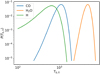 |
Fig. 1 Distribution of Gaussian binding temperatures P(Tb, X) as defined in Eq. (11) for CO (blue), water (orange), and H (green). Parameters Tb, X and σX are in Table 1. We note that there is a log–log scale. |
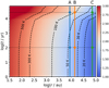 |
Fig. 2 Temperature map as a function of r and t of the physical model calculated with the radiative transfer code MOCASSIN, assuming T = Td, and where the colour bar reports log(T). The chemical network is evolved in time at each radius, varying the dust and the gas temperature according to this model, while density is a function of r only. We selected three models at three specific radii (marked A, B, and C) to discuss the impact of the multiple binding energy approach, see Fig. 3. At these radii, we further discuss the distribution of the chemical abundances at specific (r, t) combinations, indicated by the circular markers and by the horizontal dashed lines (see Fig. 4). The inner (r ≲ 3 × 10³ au) high-temperature region of the envelope is less relevant for the overall discussion, given the relatively short evaporation timescale, and for this reason it is ignored in our discussion. |
Initial abundances from Röllig et al. (2007) employed in our model in units of gas number density n.
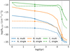 |
Fig. 3 Time evolution of rate RH, CO obtained by summing the rates of the reactions that involve the individual bins with different binding energies, as defined in Eq. (27). We note the decline of the rates with time, given by the increasing Td that evaporates more and more reactants from the surface of the grains. The models are A (blue), B (orange), and C (green), as indicated in Fig. 2, while solid and dashed lines indicate multiple- and single-bin approaches, respectively.The vertical dotted lines and the circular markers are the same as in Fig. 2, employed as a reference for Fig. 4. |
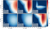 |
Fig. 4 Logarithm of RH, CO,i,j ratio with the corresponding Rref = RH, CO calculated with the single binding energy approach, for the (r, t) combinations indicated with circular markers in Figs. 2 and 3, namely cases A, B, and C (left to right panels), for t = 102 yr and t = 2.7 × 10⁴ yr (upper and lower panels). In the box, we report the dust temperature Td(r, t), t, r, and Rref in units of cm−3 s−1. The cross indicates the position of the single-case binding energy. For the sake of clarity, the colour palette lower limit is set to − 5. Compare with the sketch in Fig. 5. |
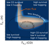 |
Fig. 5 Schematic representation of upper-right panel of Fig. 4, but also applicable to the other panels. Labels indicate the specific conditions that characterise the flux in those regions. Dashed circular lines represent the reduction of available binding sites due to the Gaussian shape of their distribution. The orange shaded area is where the flux is maximised, due to the interplay of the above conditions. |
3.2 Case study 2: the midplane of a static circumstellar disc
We applied our model to the midplane of a circumstellar disc, a denser environment when compared to the previous case, and where the temperature of the dust decreases with the distance from the star embedded in the system. We followed the minimum mass solar nebula model (MMSN; e.g. Min et al. 2011), with the following density and temperature radial profiles, where r denotes the distancefrom the central star,

with μ = 2.34, and a scale height
 (30)
(30)
where the speed of sound and the Keplerian angular frequency are, respectively,
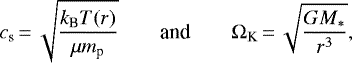 (31)
(31)
assuming M* = 1M⊙, Σ0 = 1700 g cm−2, T0 = 200 K, and where G is the gravitational constant. The dust is assumed to have the same properties as those mentioned in Sect. 3.1, while the initial abundances are the same as in Table 2, as well as the cosmic-ray ionisation rate and the visual extinction set to ζ = 5 × 10⁻¹⁷ s−1 and Av = 30 mag, respectively.
At each radius, we let the chemical abundances evolve to equilibrium, keeping the temperature and the density constant over time7. In this scenario, we are interested in determining the amount of CO and water condensed onto the dust grains at different positions of the disc. The outcome of the model is reported in Fig. 6, where the solid and the dashed lines indicate the abundance 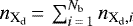 of CO (blue) and H2O (orange) with the multi- and the single-binding approach, respectively.
In this scenario, Td decreases with r, hence the abundances of the species condensed onto the grain surface increase with r, and, analogously to the previous case, the multi-binding approach retains more molecules at relatively higher temperatures, given the availability of higher binding energy sites. This behaviour is shown in Fig. 6, where H2 O ice is formed around 1.3 au in the multi-binding case and around 2 au with single binding, while CO is shifted from 90 to about 33 au, aware that the exact values depend on T0, which determines the temperature profile of the disc.
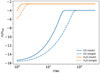 |
Fig. 6 Comparison of radial profiles of the abundances relative to the total density between single- (dashed) and multi-binding (solid) ones for CO (blue) and water (orange). The background model is the static MMSN protoplanetary disc described in the text. |
3.3 Parameter analysis
In order to avoid convergence problems, we performed our previous models with Nb = 51 bins of binding energy. However, this number affects the overall efficiency of the chemical solver, sincethe number of each evaporation/adsorption reaction is increased by a factor Nb, while the number of each surface reaction by a factor  , where M is the number of products. The effect ofchanging Nb is reported in Fig. 7 by plotting the same quantity of Fig. 3 for cases B and C and by changing the number of bins as Nb = [1, 5, 11, 21, 51]. We note that Nb = 21 reproduces the results of Nb = 51, while Nb = 11 works for B,but not for C, which presents some divergence. Case A (not reported here for the sake of clarity) shows the same behaviour as case B.
Figure 8 shows the effect of changing σX, in particular half (σX ∕2, dotted) and a quarter (σX ∕4, dash-dotted) of the original value (solid), as well as the single-binding (σX → 0, dashed). As expected, reducing this value produces results that converge to the single-binding limiting case, so σX → 0, and σX ∕4 shows a behaviour close to that of the single-binding case, suggesting that additional experiments and theoretical studies are necessary to determine P(Tb) with accuracy.
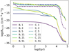 |
Fig. 7 Cases B (solid) and C (dashed) as described in Fig. 3. The different Nb in the legend are indicated with different colours. Case A is not reported for the sake of clarity, but presents similar convergence with Nb to case B. |
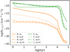 |
Fig. 8 Cases B (orange) and C (green) as described in Fig. 3. We compare σX as in Table 1 (solid), half (dotted), quarter (dash-dotted) of the value, and single case (dashed), meaning σX → 0. Case A is not reported for the sake of clarity, but presents a similar behaviour to case B. |
4 Discussion and outlook
We implemented a framework to explore the effects of a distribution of binding energies on the grain sites that participate in dust chemistry, rather than a single value, as is generally employed in chemical models. This approach is supported by recent theoreticaland experimental findings that show distributions resembling Gaussian functions.
Our results suggest that employing a distribution allows the molecules to have access to higher energy binding sites, hence increasing their residence time onto the grain surface, and then becoming available to react with other molecules, even at dust temperatures that usually present poor or no reactivity at all. We also found that, given the dust temperature, the surface reactivity is affected by the interplay of three ingredients (cf. Fig. 5):
Residence time: in the high-energy part of the binding site’s distribution P(Tb), molecules remain for longer on the grains, making them available for reactions at higher temperatures.
Thermal hopping: on the other hand, the high-energy region of P has lower hopping efficiency, hence reducing the reactivity.
Site availability: even if there are combinations of reactants with long residence times and high hopping efficiency, the reactivity is ultimately determined by the wings of P, where there are (by construction) fewer available sites where molecules can be bounded.
Our models show that the combination of these three effects is relevant in astrophysical environments, such as the gas surrounding protostars and in protoplanetary discs, with consequences on the formation of interstellar-complex organic molecules and on the location of the so-called snow lines.
In the first case, we followed the time-dependent evolution of a chemical network, which we computed alongside the variation of the dust temperature caused by the change in the protostar’s luminosity. In particular, we followed the efficiency of the reaction Hd + COd → products, finding differences that span several orders of magnitude, depending on density and temperature.
Analogously, on the midplane of a protoplanetary disc with the multi-binding approach, molecules like CO and H2 O can be found on grains at a closer distance from the central star, where the dust is relatively warmer. This determines the position of the snow lines, which play a key role in regulating the position and the characteristics of the planet-forming regions of the disc.
It is important to notice that our model follows the widely used approach that does not make a distinction between the position of the monolayers in the ice mantle. However, if we assume that deeper layers behave differently, we might obtain different results when the ice thickness increases, given that the chemistry of the bulk ice depends on cracks, mantle porosity (Mispelaer et al. 2013; Yoneda et al. 2016), and on the possible lack of bulk diffusion (Ghesquière et al. 2018; Shingledecker et al. 2019).
In conclusion, by exploring a set of astrophysical models, we found that including a multi-binding framework in chemical models leads to a substantial difference in their outcomes. However, in a practical situation, (i) the number of reactions needed for multi-binding is considerably large (affecting the computational efficiency of most of the state-of-the-art chemical models), and (ii) the exact shape of the binding energy distribution function will play a key role in the evolution of these chemical models. These two points suggest that it is crucial to find affordable solutions in order to simplify the problem from a numerical point of view and to increase the number of theoretical and experimental works to constrain the uncertainties. We also stress the need for systematic theoretical studies to build a proper database of accurate binding energy distributions, not only on ASW structure, but also on a mixture of ices and as a function of the coverage parameter.
Acknowledgements
The authors want to thank the referees for their useful comments and insights. S.B. is financially supported by CONICYT Fondecyt Iniciación (project 11170268), CONICYT programa de Astronomia Fondo Quimal 2017 QUIMAL170001, and BASAL Centro de Astrofisica y Tecnologias Afines (CATA) AFB-17002. G.B. acknowledges support from Beca de Doctorado Nacional ANID n. 21200180. S.V.G. is financially supported by ANID Fondecyt Iniciacion (project 11170949). B.E. acknowledges support from the DFG cluster of excellence “Origin and Structure of the Universe” (http://www.universe-cluster.de/). This work was funded by the DFG Research Unit FOR 2634/1 ER685/11-1.
Appendix A Chemical network
The chemical reactions employed in our models are reported in Table A.1 following Glover et al. (2010), as implemented in Grassi et al. (2017). The rate coefficients in machine-readable format can be found online8 and in Sect. 3 for surface reactions.
Chemical network employed in this paper.
References
- Bonfand, M., Belloche, A., Garrod, R. T., et al. 2019, A&A, 628, A27 [NASA ADS] [CrossRef] [EDP Sciences] [Google Scholar]
- Bovolenta, G., Bovino, S., Vöhringer-Martinez, E., et al. 2020, Mol. Astrophys., submitted [arXiv:2010.09138] [Google Scholar]
- Caselli, P. 2002, Planet. Space Sci., 50, 1133 [NASA ADS] [CrossRef] [Google Scholar]
- Collings, M. P., Anderson, M. A., Chen, R., et al. 2004, MNRAS, 354, 1133 [NASA ADS] [CrossRef] [Google Scholar]
- Cuppen, H. M., Walsh, C., Lamberts, T., et al. 2017, Space Sci. Rev., 212, 1 [Google Scholar]
- Das, A., Sil, M., Gorai, P., Chakrabarti, S. K., & Loison, J.-C. 2018, ApJS, 237, 9 [NASA ADS] [CrossRef] [Google Scholar]
- Dulieu, F., Congiu, E., Noble, J., et al. 2013, Sci. Rep., 3, 1338 [NASA ADS] [CrossRef] [Google Scholar]
- Enrique-Romero, J., Rimola, A., Ceccarelli, C., et al. 2019, ACS Earth Space Chem., 3, 2158 [CrossRef] [Google Scholar]
- Ercolano, B., Barlow, M. J., Storey, P. J., & Liu, X. W. 2003, MNRAS, 340, 1136 [NASA ADS] [CrossRef] [Google Scholar]
- Ercolano, B., Barlow, M. J., & Storey, P. J. 2005, MNRAS, 362, 1038 [NASA ADS] [CrossRef] [Google Scholar]
- Fayolle, E. C., Balfe, J., Loomis, R., et al. 2016, ApJ, 816, L28 [NASA ADS] [CrossRef] [Google Scholar]
- Fraser, H., & van Dishoeck, E. 2004, Ad. Space Res., 33, 14 [NASA ADS] [CrossRef] [Google Scholar]
- Garrod, R. T. 2008, A&A, 491, 239 [NASA ADS] [CrossRef] [EDP Sciences] [Google Scholar]
- Ghesquière, P., Ivlev, A., Noble, J. A., & Theulé, P. 2018, A&A, 614, A107 [NASA ADS] [CrossRef] [EDP Sciences] [Google Scholar]
- Glover, S. C. O., Federrath, C., Mac Low, M. M., & Klessen, R. S. 2010, MNRAS, 404, 2 [Google Scholar]
- Grassi, T., Bovino, S., Schleicher, D. R. G., et al. 2014, MNRAS, 439, 2386 [NASA ADS] [CrossRef] [MathSciNet] [Google Scholar]
- Grassi, T., Bovino, S., Haugbølle, T., & Schleicher, D. R. G. 2017, MNRAS, 466, 1259 [NASA ADS] [CrossRef] [Google Scholar]
- Hasegawa, T. I., & Herbst, E. 1993, MNRAS, 263, 589 [NASA ADS] [CrossRef] [Google Scholar]
- Hasegawa, T. I., Herbst, E., & Leung, C. M. 1992, ApJS, 82, 167 [NASA ADS] [CrossRef] [Google Scholar]
- He, J., Frank, P., & Vidali, G. 2011, Phys. Chem. Chem. Phys., 13, 15803 [CrossRef] [Google Scholar]
- He, J., Acharyya, K., & Vidali, G. 2016a, ApJ, 825, 89 [NASA ADS] [CrossRef] [Google Scholar]
- He, J., Acharyya, K., & Vidali, G. 2016b, ApJ, 823, 56 [CrossRef] [Google Scholar]
- Herbst, E., Vidali, G., & Ceccarelli, C. 2020, ACS Earth Space Chem., 4, 488 [CrossRef] [Google Scholar]
- Hocuk, S., & Cazaux, S. 2015, A&A, 576, A49 [NASA ADS] [CrossRef] [EDP Sciences] [Google Scholar]
- Hollenbach, D., & McKee, C. F. 1979, ApJS, 41, 555 [NASA ADS] [CrossRef] [Google Scholar]
- Hosokawa, T., & Omukai, K. 2009, ApJ, 691, 823 [NASA ADS] [CrossRef] [Google Scholar]
- Jin, M., & Garrod, R. T. 2020, ApJS, 249, 26 [CrossRef] [Google Scholar]
- Katz, N., Furman, I., Biham, O., Pirronello, V., & Vidali, G. 1999, ApJ, 522, 305 [NASA ADS] [CrossRef] [Google Scholar]
- Linnartz, H., Ioppolo, S., & Fedoseev, G. 2015, Int. Rev. Phys. Chem., 34, 205 [CrossRef] [Google Scholar]
- Mathis, J. S., Rumpl, W., & Nordsieck, K. H. 1977, ApJ, 217, 425 [NASA ADS] [CrossRef] [Google Scholar]
- Min, M., Dullemond, C. P., Kama, M., & Dominik, C. 2011, Icarus, 212, 416 [NASA ADS] [CrossRef] [Google Scholar]
- Mispelaer, F., Theulé, P., Aouididi, H., et al. 2013, A&A, 555, A13 [NASA ADS] [CrossRef] [EDP Sciences] [Google Scholar]
- Muñoz Caro, G. M., Jiménez-Escobar, A., Martín-Gago, J. Á., et al. 2010, A&A, 522, A108 [NASA ADS] [CrossRef] [EDP Sciences] [Google Scholar]
- Noble, J. A., Congiu, E., Dulieu, F., & Fraser, H. J. 2012, MNRAS, 421, 768 [NASA ADS] [Google Scholar]
- Penteado, E. M., Walsh, C., & Cuppen, H. M. 2017, ApJ, 844, 71 [NASA ADS] [CrossRef] [Google Scholar]
- Potapov, A., Jäger, C., Henning, T., Jonusas, M., & Krim, L. 2017, ApJ, 846, 131 [NASA ADS] [CrossRef] [Google Scholar]
- Röllig, M., Abel, N. P., Bell, T., et al. 2007, A&A, 467, 187 [NASA ADS] [CrossRef] [EDP Sciences] [Google Scholar]
- Ruaud, M., & Gorti, U. 2019, ApJ, 885, 146 [NASA ADS] [CrossRef] [Google Scholar]
- Schlemmer, S., Illemann, J., Wellert, S., & Gerlich, D. 2001, J. Appl. Phys., 90, 5410 [CrossRef] [Google Scholar]
- Shampine, L. F., & Reichelt, M. W. 1997, SIAM J. Sci. Comput., 18, 1 [CrossRef] [Google Scholar]
- Shimonishi, T., Nakatani, N., Furuya, K., & Hama, T. 2018, ApJ, 855, 27 [CrossRef] [Google Scholar]
- Shingledecker, C. N., Vasyunin, A., Herbst, E., & Caselli, P. 2019, ApJ, 876, 140 [NASA ADS] [CrossRef] [Google Scholar]
- Skouteris, D., Balucani, N., Ceccarelli, C., et al. 2018, ApJ, 854, 135 [Google Scholar]
- Skouteris, D., Balucani, N., Ceccarelli, C., et al. 2019, MNRAS, 482, 3567 [NASA ADS] [CrossRef] [Google Scholar]
- Stahler, S. W., & Palla, F. 2005, The Formation of Stars (New York: John Wiley & Sons) [Google Scholar]
- Stahler, S. W., Shu, F. H., & Taam, R. E. 1981, ApJ, 248, 727 [NASA ADS] [CrossRef] [Google Scholar]
- Stevenson, D. J., & Lunine, J. I. 1988, Icarus, 75, 146 [NASA ADS] [CrossRef] [Google Scholar]
- Tafalla, M., Myers, P. C., Caselli, P., Walmsley, C. M., & Comito, C. 2002, ApJ, 569, 815 [NASA ADS] [CrossRef] [Google Scholar]
- Taquet, V., Charnley, S. B., & Sipilä, O. 2014, ApJ, 791, 1 [NASA ADS] [CrossRef] [Google Scholar]
- Theulé, P., Endres, C., Hermanns, M., Bossa, J.-B., & Potapov, A. 2020, ACS Earth Space Chem., 4, 86 [CrossRef] [Google Scholar]
- Tielens, A. G. G. M., & Allamandola, L. J. 1987, Interstellar Processes, eds. D. J. Hollenbach, & H. A. Thronson, (Dordrecht: Springer), 134, 397 [NASA ADS] [CrossRef] [Google Scholar]
- Tielens, A. G. G. M., & Hagen, W. 1982, A&A, 114, 245 [Google Scholar]
- Vasyunin, A. I., Caselli, P., Dulieu, F., & Jiménez-Serra, I. 2017, ApJ, 842, 33 [Google Scholar]
- Wakelam, V., Loison, J. C., Mereau, R., & Ruaud, M. 2017, Molecular Astrophysics, 6, 22 [NASA ADS] [CrossRef] [Google Scholar]
- Watanabe, N., Kimura, Y., Kouchi, A., et al. 2010, ApJ, 714, L233 [NASA ADS] [CrossRef] [Google Scholar]
- Yocum, K. M., Smith, H. H., Todd, E. W., et al. 2019, J. Phys. Chem. A, 123, 8702 [CrossRef] [Google Scholar]
- Yoneda, H., Tsukamoto, Y., Furuya, K., & Aikawa, Y. 2016, ApJ, 833, 105 [NASA ADS] [CrossRef] [Google Scholar]
- Zhang, K., Blake, G. A., & Bergin, E. A. 2015, ApJ, 806, L7 [NASA ADS] [CrossRef] [Google Scholar]
Binding energy Eb and binding temperature are related by the Boltzmann constant kB. The terms “binding energy” and “binding temperature” are used in this paper interchangeably.
In principle, this number varies with the properties of the specific molecule, but the value employed here (and by other authors) does not affect our conclusions.
https://bitbucket.org/tgrassi/multi_bind, commit: 87c8a72.
Chemical reactions are listed in Appendix A and rate coefficients can be found at https://bitbucket.org/tgrassi/multi_bind/src/master/networks/
We tested our model by changing nc in the 104 to 107 cm−3 range and rc in the 104 to 105 au range, but their role in affecting our findings is negligible when compared to the role played by the variation in luminosity, the latter having the largest impact on the temperature profiles.
The code to reproduce this model can be found at https://bitbucket.org/tgrassi/multi_bind/src/master/main.py
The code to reproduce the disc model can be found at https://bitbucket.org/tgrassi/multi_bind/src/master/main_disk.py
All Tables
Initial abundances from Röllig et al. (2007) employed in our model in units of gas number density n.
All Figures
|
Fig. 1 Distribution of Gaussian binding temperatures P(Tb, X) as defined in Eq. (11) for CO (blue), water (orange), and H (green). Parameters Tb, X and σX are in Table 1. We note that there is a log–log scale. |
| In the text | |
|
Fig. 2 Temperature map as a function of r and t of the physical model calculated with the radiative transfer code MOCASSIN, assuming T = Td, and where the colour bar reports log(T). The chemical network is evolved in time at each radius, varying the dust and the gas temperature according to this model, while density is a function of r only. We selected three models at three specific radii (marked A, B, and C) to discuss the impact of the multiple binding energy approach, see Fig. 3. At these radii, we further discuss the distribution of the chemical abundances at specific (r, t) combinations, indicated by the circular markers and by the horizontal dashed lines (see Fig. 4). The inner (r ≲ 3 × 10³ au) high-temperature region of the envelope is less relevant for the overall discussion, given the relatively short evaporation timescale, and for this reason it is ignored in our discussion. |
| In the text | |
|
Fig. 3 Time evolution of rate RH, CO obtained by summing the rates of the reactions that involve the individual bins with different binding energies, as defined in Eq. (27). We note the decline of the rates with time, given by the increasing Td that evaporates more and more reactants from the surface of the grains. The models are A (blue), B (orange), and C (green), as indicated in Fig. 2, while solid and dashed lines indicate multiple- and single-bin approaches, respectively.The vertical dotted lines and the circular markers are the same as in Fig. 2, employed as a reference for Fig. 4. |
| In the text | |
|
Fig. 4 Logarithm of RH, CO,i,j ratio with the corresponding Rref = RH, CO calculated with the single binding energy approach, for the (r, t) combinations indicated with circular markers in Figs. 2 and 3, namely cases A, B, and C (left to right panels), for t = 102 yr and t = 2.7 × 10⁴ yr (upper and lower panels). In the box, we report the dust temperature Td(r, t), t, r, and Rref in units of cm−3 s−1. The cross indicates the position of the single-case binding energy. For the sake of clarity, the colour palette lower limit is set to − 5. Compare with the sketch in Fig. 5. |
| In the text | |
|
Fig. 5 Schematic representation of upper-right panel of Fig. 4, but also applicable to the other panels. Labels indicate the specific conditions that characterise the flux in those regions. Dashed circular lines represent the reduction of available binding sites due to the Gaussian shape of their distribution. The orange shaded area is where the flux is maximised, due to the interplay of the above conditions. |
| In the text | |
|
Fig. 6 Comparison of radial profiles of the abundances relative to the total density between single- (dashed) and multi-binding (solid) ones for CO (blue) and water (orange). The background model is the static MMSN protoplanetary disc described in the text. |
| In the text | |
|
Fig. 7 Cases B (solid) and C (dashed) as described in Fig. 3. The different Nb in the legend are indicated with different colours. Case A is not reported for the sake of clarity, but presents similar convergence with Nb to case B. |
| In the text | |
|
Fig. 8 Cases B (orange) and C (green) as described in Fig. 3. We compare σX as in Table 1 (solid), half (dotted), quarter (dash-dotted) of the value, and single case (dashed), meaning σX → 0. Case A is not reported for the sake of clarity, but presents a similar behaviour to case B. |
| In the text | |
Current usage metrics show cumulative count of Article Views (full-text article views including HTML views, PDF and ePub downloads, according to the available data) and Abstracts Views on Vision4Press platform.
Data correspond to usage on the plateform after 2015. The current usage metrics is available 48-96 hours after online publication and is updated daily on week days.
Initial download of the metrics may take a while.