| Issue |
A&A
Volume 643, November 2020
|
|
|---|---|---|
| Article Number | A71 | |
| Number of page(s) | 37 | |
| Section | Catalogs and data | |
| DOI | https://doi.org/10.1051/0004-6361/202037620 | |
| Published online | 05 November 2020 | |
The Gaia-ESO Survey: Calibrating the lithium–age relation with open clusters and associations
I. Cluster age range and initial membership selections⋆,⋆⋆
1
Departamento de Física de la Tierra y Astrofísica and IPARCOS-UCM, Instituto de Física de Partículas y del Cosmos de la UCM, Facultad de Ciencias Físicas, Universidad Complutense de Madrid, 28040 Madrid, Spain
e-mail: This email address is being protected from spambots. You need JavaScript enabled to view it.
2
Observatorio Astronómico Nacional (OAN-IGN), Apdo 112, 28803 Alcalá de Henares, Madrid, Spain
3
Instituto de Astrofísica e Ciências do Espaçø, Universidade do Porto, CAUP, Rua das Estrelas, 4150-762 Porto, Portugal
4
Instituto de Astrofísica de Canarias (IAC), 38205 La Laguna, Tenerife, Spain
5
Universidad de la Laguna, Dept. Astrofísica, 38206 La Laguna, Tenerife, Spain
6
INAF – Osservatorio Astrofisico di Catania, Via S. Sofia, 78 95123 Catania, Italy
7
Università di Catania, Dipartimento di Fisica e Astronomia, Sezione Astrofisica, Via S. Sofia 78, 95123 Catania, Italy
8
Institut für Astronomie und Astrophysik, Eberhard Karls Universität, Sand 1, 72076 Tübingen, Germany
9
INAF – Osservatorio Astrofisico di Arcetri, Largo E. Fermi 5, 50125 Firenze, Italy
10
Nicolaus Copernicus Astronomical Center, Polish Academy of Sciences, ul. Bartycka 18, 00-716 Warsaw, Poland
11
Observational Astrophysics, Division of Astronomy and Space Physics, Department of Physics and Astronomy, Uppsala University, Box 516, 751 20 Uppsala, Sweden
12
Institute of Astronomy, University of Cambridge, Madingley Road, Cambridge CB3 0HA, UK
13
Lund Observatory, Department of Astronomy and Theoretical Physics, Box 43 221 00 Lund, Sweden
14
INAF – Osservatorio Astronomico di Palermo, Piazza del Parlamento, 1, 90134 Palermo, Italy
15
Dipartimento di Fisica e Astronomia, Università di Padova, Vicolo dell’Osservatorio 3, 35122 Padova, Italy
16
Spanish Virtual Observatory, Centro de Astrobiología (INTA-CSIC), PO Box 78, 28691 Villanueva de la Cañada, Madrid, Spain
17
Departamento de Ciencias Físicas, Universidad Andrés Bello, Fernández Concha 700, Las Condes, Santiago, Chile
18
Dipartimento di Fisica “E. Fermi”, Università di Pisa, Largo Bruno Pontecorvo 3, 56127 Pisa, Italy
19
INAF – Padova Observatory, Vicolo dell’Osservatorio 5, 35122 Padova, Italy
20
Instituto de Física y Astronomía, Universidad de Valparaíso, Valparaíso, Chile
21
Núcleo Milenio Formación Planetaria – NPF, Universidad de Valparaíso, Valparaíso, Chile
22
Núcleo de Astronomía, Facultad de Ingeniería y Ciencias, Universidad Diego Portales (UDP), Santiago, Chile
23
Instituto de Astrofísica de Andalucía (CSIC), Glorieta de la Astronomía s/n, 18008 Granada, Spain
24
Dipartimento di Fisica e Astronomia Galileo Galilei, Vicolo Osservatorio 3, 35122 Padova, Italy
Received:
29
January
2020
Accepted:
29
July
2020
Abstract
Context. Previous studies of open clusters have shown that lithium depletion is not only strongly age dependent but also shows a complex pattern with other parameters that is not yet understood. For pre- and main-sequence late-type stars, these parameters include metallicity, mixing mechanisms, convection structure, rotation, and magnetic activity.
Aims. We perform a thorough membership analysis for a large number of stars observed within the Gaia-ESO survey (GES) in the field of 20 open clusters, ranging in age from young clusters and associations, to intermediate-age and old open clusters.
Methods. Based on the parameters derived from the GES spectroscopic observations, we obtained lists of candidate members for each of the clusters in the sample by deriving radial velocity distributions and studying the position of the kinematic selections in the EW(Li)-versus-Teff plane to obtain lithium members. We used gravity indicators to discard field contaminants and studied [Fe/H] metallicity to further confirm the membership of the candidates. We also made use of studies using recent data from the Gaia DR1 and DR2 releases to assess our member selections.
Results. We identified likely member candidates for the sample of 20 clusters observed in GES (iDR4) with UVES and GIRAFFE, and conducted a comparative study that allowed us to characterize the properties of these members as well as identify field contaminant stars, both lithium-rich giants and non-giant outliers.
Conclusions. This work is the first step towards the calibration of the lithium–age relation and its dependence on other GES parameters. During this project we aim to use this relation to infer the ages of GES field stars, and identify their potential membership to young associations and stellar kinematic groups of different ages.
Key words: open clusters and associations: general / stars: late-type / stars: abundances / techniques: spectroscopic
Based on observations collected with ESO telescopes at the La Silla Paranal Observatory in Chile, for the Gaia-ESO Large Public Spectroscopic Survey (188.B-3002, 193.B-0936).
All tables in Appendix C are only available at the CDS via anonymous ftp to cdsarc.u-strasbg.fr (130.79.128.5) or via http://cdsarc.u-strasbg.fr/viz-bin/cat/J/A+A/643/A71
© ESO 2020
1. Introduction
Lithium is a very fragile element that is easily destroyed in stellar interiors, burning at temperatures above ∼2.5 × 10⁶ K, corresponding to the temperature at the base of the convective zone of a solar-mass star on the zero-age main sequence (ZAMS; Siess et al. 2000). For this reason, lithium is slowly being depleted and its surface abundance decreases over time in solar-type and lower mass stars (Jeffries et al. 2014; Bouvier et al. 2016; Lyubimkov 2016). According to standard stellar models, low-mass stars show lithium depletion increasing with decreasing mass, while stars more massive than the Sun undergo little or no depletion, and very low-mass stars show no depletion at all, given that their central temperature never reaches the Li burning point (Jones et al. 1999). An additional contribution of surface lithium abundance can also be detected for some stars, such as Li-rich giants. Given the low stellar temperatures necessary to destroy lithium in stellar interiors, these Li-rich stars would require extra non-standard mixing mechanisms to account for the additional lithium detected on their surfaces (see Sect. 4).
Because it only survives in the outer layers of a star1, lithium is a very sensitive tracer of stellar evolution and non-standard mixing mechanisms in stellar interiors (see e.g., Sestito & Randich 2005; Castro et al. 2016), and is particularly relevant for studies of the evolution of low-mass stars and for the determination of the age of stellar clusters. Cluster ages determined in this way are less subject to systematic uncertainties than ages derived from other methods (e.g., Hobbs & Pilachowski 1986; Oliveira et al. 2003; Soderblom et al. 2014).
As most stars do not form individually, but inside clusters and associations, the study of clusters of different ages (from a few Myr to several Gyr) and chemical compositions is essential to understand star formation and evolution. In addition to this, open clusters are very useful tracers when studying the formation and evolution of the Galaxy, especially the spatial distribution of elemental abundances in the Galactic thin disc and their evolution with time (e.g., Friel 1995; Smiljanic et al. 2014; Magrini et al. 2015; Netopil et al. 2016; Casali et al. 2019).
While standard models of stellar evolution including convection as the only mixing mechanism (e.g., Soderblom et al. 1990) predict that stellar Li abundances should only be a function of effective temperature and age, observations of solar and late-type stars in open clusters of different ages show that lithium depletion depends also on a series of other factors, such as metallicity, rotation, mixing mechanisms, convection structure, mass loss and magnetic activity (e.g., Deliyannis et al. 1990; Soderblom et al. 1993; Ventura et al. 1998; Jones et al. 1999; Randich et al. 2002; Charbonnel & Talon 2005; Pallavicini et al. 2005; Bouvier 2008). This indicates the presence of additional non-standard mixing processes, such as rotational mixing, diffusion, mass loss or gravitational waves, in addition to convection (e.g., Duncan 1981; Soderblom et al. 1995; Pallavicini et al. 1997). Even though a large amount of theoretical and observational work has been dedicated to the understanding of Li and its evolution (e.g., Sestito & Randich 2005), current available data have shown a complex pattern of Li depletion in pre- and main-sequence stars that is not yet understood. The most precise way to calibrate these effects is to conduct a comprehensive study of stellar groups with similar ages, such as open clusters, associations, and kinematic groups.
In the present work we use lithium, among other criteria, to constrain the cluster membership of a series of open clusters and associations using data from the Gaia-ESO Survey (GES). The membership analysis and calibration of the ages of open clusters and associations is of great importance to study the lithium–age relation (Soderblom 1983, 2010), which will allow us to use lithium as an effective age indicator for the field stars from GES whose age is still unknown. Thus, the ultimate aim of this project, which will continue in a separate forthcoming paper (see Sect. 7), is to use the spectroscopic observations obtained by GES for a large number of stars in a wide sample of open clusters and associations in order to apply this analysis of cluster membership to calibrate this lithium–age relation and establish its dependence on other parameters that can also be derived from the GES observations. With this ultimate aim, we focus in this work on presenting an analysis of membership for a data sample of 20 GES open clusters.
The Gaia-ESO Survey (GES – Gilmore et al. 2012; Randich et al. 2013)2 is a large public spectroscopic survey that provides a homogeneous overview of the distribution of kinematics, dynamical structure and chemical compositions in the Galaxy (Bergemann et al. 2014; Smiljanic et al. 2014). The survey uses the multi-object spectrograph FLAMES on the Very Large Telescope (ESO, Chile) to obtain high-quality, uniformly calibrated spectroscopy of about 105 stars, plus a sample of about 100 open clusters (OCs) and star-forming regions (SFRs) of all ages, metallicities and stellar masses3. GES is unique among other surveys for its depth, its UVES observations, and its comprehensive data for open clusters. Combined with precision astrometry provided by Gaia, delivering accurate parallaxes and proper motions, GES provides a rich dataset yielding 3D spatial distributions, 3D kinematics, chemical abundances, and improved fundamental parameters for all target objects (e.g., Beccari et al. 2018; Cantat-Gaudin et al. 2018; Randich et al. 2018; Roccatagliata et al. 2018; Soubiran et al. 2018; Cánovas et al. 2019; Bossini et al. 2019).
This paper is organised as follows. In Sect. 2 we discuss the GES target selection and describe the spectral measurements we initially took using the available GES data. Section 3 describes our criteria on radial velocities (RV), atmospheric lithium content, surface gravity, and metallicity to identify likely cluster members. In Sect. 4 we discuss the selection of giant and non-giant (NG) outlier contaminants also obtained during the membership process. In Sect. 5 we present our lists of candidate members for all clusters studied here (individual cluster notes with more detailed information on the membership process for each of the pre-selected clusters can be also found in Appendix A). In Sect. 6 we present some further discussion of our results. Finally, we summarise our results and discuss our future work as part of this project in Sect. 7.
2. Data
GES observations are performed with the optical spectrograph FLAMES at the VLT (Pasquini et al. 2002), providing both high-resolution spectra with UVES (R = 47 000) of mainly single FGK stars (e.g., Smiljanic et al. 2014; Frasca et al. 2015; Lanzafame et al. 2015), and medium resolution spectra with GIRAFFE (R = 5500–6500) of late-type (F to M) stars in the PMS (pre-main sequence) or MS phase. The GIRAFFE/HR15N setup is particularly useful when it comes to the study of young stars considering that it covers both Hα and Li (6707.84 Å) spectral regions. However, fundamental parameters such as Teff, log g and [Fe/H] are less well determined in this wavelength range than in other settings (e.g., Lanzafame et al. 2015). The WG10 and WG11 GES working groups (WGs) are focused on the spectroscopic analysis of the GIRAFFE and UVES FGK stars, respectively (e.g., Gilmore et al. 2012; Sacco et al. 2015), while WG12 is dedicated to the analysis of stars in the fields of young clusters using both UVES and GIRAFFE data.
The analysis is performed in cycles, after the reduction of new spectra observed by GES. Recommended parameters are defined by improving upon each new analysis by means of updated input and methods using a calibration strategy described in Pancino et al. (2017). At the end of each cycle, and after additional internal checks are made following the data homogenisation, an internal data release (iDR) is produced and made available to the GES consortium (e.g., Lanzafame et al. 2015). The last internal data releases (iDR5, iDR6) include all the data derived from the observations collected until the completion of the survey, in January 2018.
For all the following analysis presented in this paper we used the data provided by the fourth internal data release of GES (iDR4). iDR4 is a full internal release within the GES consortium available since February 2016, containing recommended parameters, derived products (such as individual element abundances or chromospheric activity), and radial and rotational velocities for 38 clusters, both open and globular. We also note that we decided to wait until iDR6 had been fully released instead of upgrading our analysis with the iDR5 data (see Sect. 7). We consider that there is not an appreciable difference between iDR4 and iDR5 (as opposed to iDR4 versus iDR6) in regards to for example the number of clusters present in the release: there are 47 clusters in iDR5 versus 38 in iDR4 – only 9 additional clusters, compared to the total of 80 in iDR6, 42 more than in iDR4. We also note that, seeing as we focus in this study on FGK stars, we discarded all stars with Teff > 7500 K from the iDR4 sample.
The output parameters resulting from the spectroscopic analysis of GES WGs are divided into raw, fundamental and derived parameters: Raw parameters such as Hα emission and Li equivalent widths (EWs) are directly measured on the input spectra. Their values are used in the case of groups such as WG12 to optimise the evaluation of the fundamental parameters (Teff, log g, [Fe/H], projected rotational velocity (v sin i), veiling (r), and the gravity-sensitive spectral index γ, Damiani et al. 2014). Lastly, derived parameters (such as elemental abundances and chromospheric activity indices), are those that require prior knowledge of the fundamental parameters. Smiljanic et al. (2014) derived parameters for UVES spectra of FGK stars, while Lanzafame et al. (2015) did the same specifically for PMS stellar spectra.
As part of the analysis of iDR4 data conducted by the GES UCM node (Lanzafame et al. 2015), during the course of this study we analysed the UVES spectra and manually measured the EWs of Li Iλ6707.76 and adjacent Fe Iλ6707.43 lines (EW(Fe)). The initial EWs of these lines were measured with the automatic tool TAME (Tool for Automatic Measurement of Equivalent Widths – Kang & Lee 2012; Tabernero et al. 2019). This tool allowed us to discard all spectra with EW(Li) < 5 mÅ. We then performed an individual analysis of each of the remaining spectra by measuring the EW(Li) and EW(Fe) manually with the IRAF task splot (e.g., Smiljanic et al. 2014; Lanzafame et al. 2015), using the TAME values for comparison purposes. With enough resolution (among other factors such as the lack of broadening because of rotation), the Li line and the nearby blends are distinguishable, and EW(Li) and EW(Fe) can be measured individually, deblending and adopting a Gaussian fitting to the line profile. However, in the case of lower resolution spectra only EW(Li I + Fe I) can be measured. EWs were corrected as EW(Li) =EW(Li I + Fe I)−EW(Fe) in those cases where the Li and Fe lines could not be resolved. EW(Fe) was estimated using the ewfind driver within MOOG code (Sneden 1973) and adopting the recommended stellar parameters4. We also made use of the lithium measurements derived by the OACT (Osservatorio Astrofisico di Catania) node, adding to our cluster calibration analysis a number of GIRAFFE stars with no recommended EW(Li) values in iDR4. This has been especially important regarding the intermediate-age and old clusters considered in this study, for which only a few UVES Li values were listed in the iDR4 sample.
Our present sample from iDR4 includes 12493 UVES and GIRAFFE spectra of 20 open clusters of ages ranging from 1 Myr to 5 Gyr. Given the nature of our particular study, we discarded the 12 old globular clusters out of the 38 clusters in iDR4, as lithium cannot be used as a youth indicator in those cases. Of the remaining 26 we also discarded six young and intermediate open clusters during our analysis (NGC 2264, NGC 2451, NGC 3532, NGC 3293, NGC 6530, and Trumpler 14) as a result of the data suffering from the contamination of nebular lines, which could affect the RV distributions and therefore our membership analysis (Klutsch et al., in prep.)5. The remaining 20 clusters that constitute our sample include two SFRs (1–3 Myr) and five young clusters (10–38 Myr) with no nebulosity issues, along with three intermediate clusters (251–500 Myr), and ten old clusters (0.8–5 Gyr). In Sect. 3 we discuss the membership criteria followed to present the lists of initial candidate members of all the clusters included in the sample.
A number of membership studies have already been conducted and the authors identified potential members from the GES data for most of the 20 clusters selected in the present paper (Table 1). These studies have been of great use to evaluate the goodness of our membership analysis by comparing our final candidates with previous membership lists. Table 1 also lists the age estimates and mean metallicities from the literature for all clusters. We divided the sample clusters into groups according to age: young (1–50 Myr), intermediate (50–700 Myr), and old clusters (> 700 Myr). As shown in the table, we differentiate between publications that include membership studies, and the few that only mention them and/or study them without taking membership analysis primarily into account. In the individual notes of Appendix A, where we present our results of cluster membership, we reference these studies in more detail for each of the clusters. These previous GES studies also provided their mean properties. In particular we made use of their mean ages (Table 1), RVs (Table 2), and metallicities (Tables 1 and 3).
Age estimates, mean metallicity, distance to the Sun, and GES membership studies from the literature for the 20 clusters in our sample.
Fit parameters and RV members for the sample clusters.
Fit parameters and metallicity membership for the sample clusters.
3. Selection criteria and membership analysis
To obtain final lists of candidate members for the 20 clusters in our sample, we conducted a homogeneous and coherent analysis of their membership according to the following criteria:
-
RV analysis (Sect. 3.1): We selected the RV candidates by fitting the radial velocity distributions derived from GES for each cluster using a two-sigma clipping method.
-
Li content (Sect. 3.2): Any RV candidate is considered a potential lithium member according to its locus in the EW(Li)-versus-Teff diagrams.
-
Gravity indicators (Sect. 3.3): We use the Kiel (log g-versus-Teff) diagram to identify outliers, such as lithium-rich giant stars and other field contaminants, which we disregard hereafter during our analysis. In the case of young clusters, we mainly use the gravity indicator γ to effectively discard giant contaminants.
-
Metallicity (Sect. 3.4): An analysis of the metallicity distributions for each cluster provides confirmation of the membership of the candidate stars.
-
Gaia studies (Sects. 3.5 and 5): Finally, we made use of additional studies conducted from Gaia DR1 and DR2 data (Cantat-Gaudin et al. 2018; Randich et al. 2018; Soubiran et al. 2018; Bossini et al. 2019; Cánovas et al. 2019) to further confirm our candidate selections.
Regarding the order of criteria, for the young clusters, due to their appreciable field contamination, we discarded all giant contaminants using the γ index before performing the RV analysis and obtaining lithium members. In addition, for the intermediate-age and old clusters, we relied more on the study of their metallicity distribution to ascertain final members from the initial RV candidates, as a result of the increasing difficulty in using lithium as a relevant criterion in this age range.
We also note that for all clusters we identified and discarded a series of SB1 and SB2/3/4 binary stars, which can add significant contamination to our analysis. SB1s were excluded from our kinematic analysis as they can strongly affect the observed RV distributions, but we included them in the rest of our membership analysis as lithium measurements are not affected. On the other hand, SB2/3/4s were fully discarded from our data sample for all clusters. These binary stars were identified using the iDR4 data release metadata, as well as existing studies (Merle et al. 2017, 2020).
3.1. Kinematic selection
Despite the fact that the spectroscopic targets in the field of the clusters we are studying were photometrically selected to be likely members, the GES sample also suffers from significant field star contamination. Many of these outliers can be separated from the cluster stars on the basis of their RVs (e.g., Cantat-Gaudin et al. 2014; Friel et al. 2014). Thus, the analysis of the distributions of radial velocity is decisive for estimating the cluster membership on the basis of a first selection of their potential kinematic candidates.
We obtained RV candidates for each cluster by studying each of the velocity distributions of the RV measurements that were derived from both the UVES and GIRAFFE spectra. First, we discarded initial field outliers at the tails of each of the RV distributions using the RStudio6boxplot command7. We then fitted a Gaussian curve to the resulting distribution by applying an iterative two-sigma clipping procedure on the median (e.g., Donati et al. 2014b; Friel et al. 2014). In the same way as the analysis carried out by studies such as Friel et al. (2014), we minimise the influence of the field star contaminants that could affect the estimate of the average value by relying on the median of the distribution, a more robust measure of the cluster velocity than the mean, which is more significantly affected by the presence of outliers in the distribution. After convergence is reached8, this method results in final average velocities and dispersions for each cluster. We consider as RV members all stars with RVs lying within 2σ from the average cluster velocity provided by the fit. In the specific case of those clusters that display two peaks in their RV distributions (γ Vel and NGC 2547), we note that we relied primarily on the member selections presented in the literature (Damiani et al. 2014; Jeffries et al. 2014; Spina et al. 2014b; Frasca et al. 2015; Sacco et al. 2015; Prisinzano et al. 2016; Cantat-Gaudin et al. 2018; Randich et al. 2018), as explained in Sect. 5.
For the remaining 18 clusters analysed here, Table 2 presents the mean velocity, dispersion, and RV membership intervals rendered by each fit, as well as the number of resulting RV members. After applying all membership criteria we also obtained mean RVs and dispersions for the velocity distributions of the final candidates for all clusters. For each cluster studied, our mean RV value is in agreement with that reported in the literature, as shown in Table 1. While every study made use of their own methods and criteria, a comparison with these previous literature values can be useful for further assessing the goodness of our results. We also note that, depending on a series of factors, from the number of stars in the sample to the quality of the data, some distributions exhibit more dispersion than others, and thus, larger values of σ, even after discarding field outliers with the two-sigma-clipping procedure. However, the velocity intervals, defined by σ to ascertain whether or not the stars of the sample are RV members, do include in all cases the reference RV values from the literature for each cluster. Along with this, we subsequently identified and discarded any contaminants among our kinematic selections by applying additional membership criteria.
As an example, Fig. 1 displays the RV histogram at different stages of the analysis leading to the selection of sources belonging to the one of the clusters in our sample, intermediate-age cluster NGC 6705. The top panel shows the initial RV distribution for all GES targets in this cluster field. The distribution is broad, an indicator of contamination by field outliers, and presents an increasing dispersion with distance far away from the cluster centre, where the contaminants dominate. The red markings provide an additional visualisation of how the data points are spread out. The middle panel exemplifies how we discarded a series of field stars with the RStudio boxplot tool, as a result of which the distribution becomes less broad at smaller distances, with the cluster members starting to predominate over the field contaminants (e.g., Friel et al. 2014). Finally, the bottom panel shows the fitted RV distribution following the two-sigma clipping procedure around the median. The solid line indicates the Gaussian fit of the peak of the distribution, which identifies the signature of the cluster with respect to the field contaminants, and gives the central mean velocity and dispersion σ. Figure 2 displays the RV distribution and Gaussian fit of the final candidate selection for NGC 6705, after applying all criteria resulting from our membership analysis. We report all the mean RV values and their associated dispersions in Table 2, and we also present the kinematic distributions for all clusters in our sample in Appendix B.
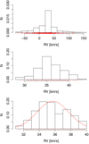 |
Fig. 1. Distribution of radial velocities and RV selection for stars in the field of the cluster NGC 6705. Top panel: initial RV distribution for all the GES sources. We discard a few contaminants at the tails using the RStudioboxplot command (middle panel), and we show the Gaussian fit of the peak of the distribution using the 2σ clipping procedure around the median (bottom panel). |
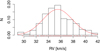 |
Fig. 2. Gaussian fit of the RV distribution of the members of the cluster NGC 6705 resulting from our membership analysis. |
Regarding the young clusters, we also recall that we discarded all giant contaminants using gravity indicators (Sect 3.3) before applying any other criteria, due to the large number of outliers in these fields. Thus, we only took the NG stars in the sample into account to study the velocity distribution and obtain RV members9. This initial filter minimised the presence of field outliers and appreciably reduced the dispersions of the velocity distributions, which resulted in improved values of σ obtained from the Gaussian fits.
3.2. Lithium members
As mentioned in the introduction, lithium is a powerful membership indicator and of great use in determining the age of clusters. Given that Li starts to be depleted during the PMS phase and that young FGK stars seem to always show a strong lithium feature (e.g., Soderblom 2010), the presence of lithium in stellar spectra is a relevant indicator of youth in late-type stars10. However, a few G/K giants may also have large Li content, and contamination by Li-rich field giants therefore remains possible (e.g., Smith et al. 1995). In the case of clusters older than 50 Myr, we subsequently discarded these giants with the aid of gravity indicators (see Sects. 3.3 and 4).
In this study we consider EW(Li) as one of the principal criteria in our analysis to select probable cluster members. We obtain the Li members of each cluster by studying the position of the RV candidates in EW(Li)-versus-Teff figures with a series of Li envelopes as a guide. We use the upper lithium envelope of IC 2602 (35 Myr) (Montes et al. 2001), the upper (Neuhaeuser et al. 1997) and lower (Soderblom et al. 1993) envelopes of the Pleiades (78–125 Myr), and the upper envelope of the Hyades (750 Myr) (Soderblom et al. 1993). These envelopes delimit the region populated by member stars in well-known open clusters covering a large range of ages. Given that various studies have already obtained age estimates for the clusters we are studying, we can distinguish the bona-fide cluster members from the Li-rich contaminants and other field stars by studying their position in the EW(Li)-versus-Teff diagram with respect to the Li envelopes.
As an example, Fig. 3 shows the EW(Li)-versus-Teff diagram for the 35 Myr young cluster IC 2602. As described above, Li members were selected by studying the position of the RV selection with respect to the IC 2602 envelope. We disregard the stars lying above the IC 2602 envelope, which are younger than 35 Myr, and those at the bottom of the figure, which are older than the cluster members. In this specific case, we can also compare the position of the Li candidates and final selection for IC 2602 with the corresponding Li envelope for the same cluster. We later applied our gravity criteria to distinguish the giant and NG outliers with Li, as shown in the figure for completeness (see Sects. 3.3 and 4). We present the EW(Li)-versus-Teff diagrams for all clusters in our sample in Appendix B.
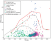 |
Fig. 3. EW(Li)-versus-Teff diagram showing the final candidate selection (red squares) for IC 2602, a 35-Myr-old cluster. The upper envelope of EW(Li) for the cluster IC 2602 is shown in red; the upper and lower envelopes of the Pleiades cluster are shown in grey; and the turquoise line represents the upper envelope of the Hyades cluster. For completeness we show here all field contaminants of interest, colour-coded as follows: RV non-members (open grey squares), Li-rich giants (blue), giant outliers which are not Li-rich, and finally (fuchsia), NG non-members (green) and possible candidates (turquoise). For more details, we refer the readers to Sects. 3.3 and 4). |
We note that, in the case of the SFRs (age ≤5 Myr), EW(Li) values can be underestimated in stars with a strong mass accretion rate due to the veiling factor (Frasca et al. 2015). Following the criterion applied by Sacco et al. (2017), for the two SFRs in our sample we considered as members all accretors with Hα10% > 270–300 km s−1 (White & Basri 2003)11, regardless of whether they are Li members or not. On the other hand, for intermediate-age and especially old clusters it becomes harder to ascertain the membership of the cluster candidates by relying on their lithium content. In these cases, the criteria on surface gravity and metallicity take on even greater importance when carrying out our membership analysis.
3.3. Gravity indicators: Kiel diagram and γ index
We made use of the Teff and log g GES spectroscopic parameters to study the (Teff, log g) plane (also known as the Kiel diagrams) for each of the 20 pre-selected clusters. Among our candidates we identified the giant stars in the field of the clusters thanks to their locus on the Kiel diagrams. This is especially helpful to exclude evolved field contaminants for which we were not able to establish a secure membership based on lithium. We consider all stars with log g < 3.5 to be likely giants, while the Li-rich giants are giant stars with A(Li) > 1.5 (see Sect. 4) for more details). For all clusters we made use of the PARSEC isochrones (Bressan et al. 2012), with Z = 0.019 (except for the very low metallicity cluster NGC 2243, where we used isochrones with Z = 0.006), and ages ranging from 1 Myr to 5 Gyr. As an example, in Fig. 4 we present the Kiel diagram for the cluster NGC 6705, while the Kiel diagrams for all clusters in our sample are in Appendix B.
 |
Fig. 4. Kiel diagram of the GES sources (open squares) in the field of the cluster NGC 6705 (300 Myr). We indicate the candidate members with red squares, while the other coloured squares denote additional field contaminants of interest: Li-rich giants (blue), (non-Li-rich) giant outliers (fuchsia), and NG non-members with Li (green). We overplot the PARSEC isochrones for a metallicity of Z = 0.019 at 200 Myr (turquoise curve), 300 Myr (blue curve), 400 Myr (green curve), and 1 Gyr (gray dashed curve). |
As the recommended log g values are often missing for the young stars in the field of clusters younger than 50 Myr when observed with the GIRAFFE setups, we made use of the γ index defined by Damiani et al. (2014) and provided by the Consortium. This index is another efficient gravity indicator for the GIRAFFE targets observed with HR15N, allowing a clear separation between low-gravity giants (γ ≥ 1), and higher gravity stars for spectral types later than G in the MS and PMS (γ ≤ 1), as shown by Spina et al. (2017). By plotting the γ index of the Li candidate members as a function of the stellar effective temperature, we have an alternative method to identify giant background stars that we excluded before applying the other membership criteria. As in previous works (e.g., Damiani et al. 2014; Delgado Mena et al. 2016; Spina et al. 2017), we classify as Li-rich background giants all stars with effective temperatures lower than 5200 K, A(Li) > 1.5, and γ > 1.01. In Fig. 5 we show as an example the γ-versus-Teff diagram for the young cluster Cha I, where the dashed lines (at Teff = 5200 and γ = 1.01) delimit the locus of the giant background stars. This region is clearly separated from the main sequence and pre-main sequence member stars. The other γ-versus-Teff diagrams of the young clusters in our sample are displayed in Appendix B.
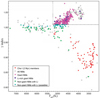 |
Fig. 5. Gravity-sensitive spectral index γ as a function of Teff for the sources (open squares) in the field of the SFR Cha I. The candidate members of Cha I are marked in red squares, while the other coloured squares denote the field contaminants of interest: Li-rich giants (blue), (non-Li-rich) giant outliers (fuchsia), NG non-members with Li (green), and potential NG outliers (turquoise – i.e., those in the 1.01 > γ > 1.0 range, see Sect. 4). As indicated by the dashed lines, we classified any stars with Teff < 5200 K and γ > 1.01. as giants. |
3.4. Metallicity
We have also taken the metallicity of the clusters into account to identify additional non-members. We use the spectroscopic index [Fe/H] derived from the GES analysis as a proxy of the metallicity. Using the [Fe/H] histograms. we search for stars with metallicities too far away from the mean cluster value. Given the homogeneity of cluster member stars, these stars are likely outliers. As an example we show the metallicity distribution for cluster NGC 6705 plotted in Fig. 6. As we mention in Sect. 3.2, the lithium criterion is less relevant when analysing older clusters, as it becomes harder to ascertain the membership of RV candidates based on their position in the EW(Li)-versus-Teff diagram. Therefore, for these clusters we relied more heavily on their metallicity distributions to discard outliers.
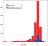 |
Fig. 6. Histogram of [Fe/H] values for all the GES stars (red) in the field of the cluster NGC 6705, as well as the candidate members (blue) resulting from our analysis. The histogram shows an increasing dispersion towards the tails, confirming that this initial distribution is dominated by field stars. |
Similarly to the selection of RV members (see Sect. 3.1), for the metallicity analysis we fitted the initial [Fe/H] distribution for each cluster (including all stars in the field before applying other membership criteria), to obtain probable metallicity candidates. For the young clusters we only took the NG stars into account to study the [Fe/H] distribution and obtain metallicity members, because of the high field contamination. We fitted each of the distributions by applying a 2σ clipping procedure on the median and adopting a 2σ limit about the cluster mean [Fe/H] yielded by the Gaussian fit to identify the most likely metallicity members. Thus, stars that are members on the basis of all the former criteria but show [Fe/H] values visibly far from the cluster average in the distribution were classified as non-members and disregarded afterwards. Figure 7 shows an example of the [Fe/H] distribution analysis for cluster NGC 6705, comparing the initial fit following the 2σ clipping procedure, from which we obtain metallicity membership limits, with the final distribution of the metallicities of the final candidates for the cluster.
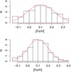 |
Fig. 7. Distributions of [Fe/H] and Gaussian fits for the intermediate-age cluster NGC 6705. We display the histogram both for sources resulting from the 2σ clipping procedure on all the GES sources in this field (top panel), and for likely cluster members after applying all of our membership criteria (bottom panel). |
Unlike the UVES metallities, the [Fe/H] values derived from the GIRAFFE spectra are widely dispersed and subject to larger uncertainties that contribute to broadening the distributions, which is a result of the lower resolution spectroscopy of the setups selected during the Survey (e.g., Spina et al. 2014b). Because the metallicity and gravity criteria are less reliable for GIRAFFE targets, we also accepted as candidates for the intermediate-age and old clusters a number of GIRAFFE Li members with [Fe/H] values outside the 2σ limit from the cluster mean provided by our fit (this was done case by case, as described in more detail in the individual notes of Appendix A, although we also consider a maximum threshold for all instances). For this reason, we also used existing membership studies from the literature to ascertain the membership of possible GIRAFFE candidates. For more details regarding specific clusters, we refer the reader to the individual notes in Appendix A and the tables in Appendix C.
We show the results of the analysis of the metallicity distributions for all clusters in Table 3, including the mean [Fe/H], dispersion and membership intervals rendered by each fit. As in the case of RV distributions, we then fitted the metallicity distributions of our final selections of candidate members for each cluster and compared the central mean [Fe/H] and its dispersion with those present in the literature (also shown in Table 1). We find that our estimates mostly agree with the literature, with the exception of a few clusters (ρ Oph, Cha I, Pismis 18 and M67, see Table 3). A possible explanation for this could be related to the lower accuracy on the [Fe/H] values derived from GIRAFFE spectra (see the individual notes in Appendix A for more details on this matter). However, it is worth noting that the literature values of [Fe/H] are obtained with different methods and from different datasets. Thus, we only conduct qualitative comparisons of these measures with those obtained from the homogeneously measured iDR4 sample, which does not consist of a means of firmly assessing the membership of our final candidates.
3.5. Gaia studies
To assess the relevance of our selections and to aid in the confirmation of our final candidates, we made use of the recent membership studies that were conducted from the Gaia-DR1 (Randich et al. 2018) and Gaia-DR2 (Cantat-Gaudin et al. 2018; Cánovas et al. 2019) data.
Randich et al. (2018) combined the parallaxes and proper motions in the Gaia-DR1 TGAS catalogue and the spectroscopic information from the iDR4 GES data for eight open clusters to calibrate stellar evolution and ages. Six of them are included in our data sample (namely, NGC 2547, IC 2391, IC 2602, IC 4665, NGC 2516 and NGC 6633). As well as considering an astrometric membership selection, these latter authors derived the cluster membership probabilities for the GES targets and used several spectroscopic tracers similar to ours: GES stars are required to have values of Teff, RVs (and v sin i when possible), and log g or γ index, as well as EW(Li) measurements. Candidates were selected based on criteria such as lithium content and RV membership probabilities, and contaminants were also discarded based on gravity, low metallicity or slow rotation. Cantat-Gaudin et al. (2018) used the astrometry data provided by the Gaia-DR2 release and applied an unsupervised membership assignment code (UPMASK) to list members and derived mean properties for 1229 clusters. Fourteen of the pre-selected 20 clusters are included in Cantat-Gaudin et al. (2018) (namely, NGC 2547, IC 2391, IC 2602, IC 4665, NGC 2516, NGC 6705, NGC 4815, NGC 6633, Berkeley 81, NGC 6005, NGC 6802, Trumpler 20, Berkeley 44, and NGC 2243). In contrast to Randich et al. (2018), this study makes use of the Gaia data alone and does not consider any spectroscopic criteria during the membership analysis. Cánovas et al. (2019) also used Gaia-DR2 astrometric measurements to study the young cluster ρ Oph, applying density-based clustering algorithms to select candidate members and identify potential new members.
In the end, we took advantage of these three studies to indirectly consider Gaia astrometry as a criterion to confirm the candidates from our spectroscopic analysis as members of each of the 17 clusters in common. For each of the clusters considered in these studies, see the cluster individual notes in Appendix A for more details regarding the comparison between the candidates listed in the Gaia studies and our final member selections. In the tables of Appendix C we also include for reference these Gaia membership selections alongside the columns listing the results of our membership analysis criteria.
Finally, when available, we adopted the ages revised by Bossini et al. (2019) for six of our clusters, which are mainly the young ones, and the RVs from Soubiran et al. (2018) for 17 of them, as reported in Tables 1 and 2, respectively. We also observed that, judging by the updated Gaia ages, as well as the apparent Li envelopes of our candidates, it is possible that some of the former age estimates for the pre-selected intermediate-age and old clusters could be overestimates – NGC 6005, for example, had a former age estimate of 1.2 Gyr, while Bossini et al. (2019) gives a lower age of 973 ± 5 Myr, which is more in accordance with the Li envelope of our candidate selection.
4. Identification of giant and NG contaminants
The study of Li-rich giants is of great interest because even though they can be found ubiquitously in a number of different environments – from open clusters, to globular clusters, the Galactic Bulge, and even dwarf galaxies (e.g., Smiljanic et al. 2016, and references therein) –, most of them are still not well understood. The existence and properties of these stars contradict expectations from standard stellar evolution models (those which only include convection as a mixing mechanism), and would need additional mechanisms that explained a supplemental contribution of surface Li abundance (e.g., Casey et al. 2016; Smiljanic et al. 2018). Li-rich giants comprise approximately 1–2% of FGK giants (e.g., Lyubimkov 2016; Smiljanic et al. 2016; Gao et al. 2019, and references therein), and are defined as those that have A(Li) ≥ 1.5 (Iben 1967; Cameron & Fowler 1971; Lagarde et al. 2012; Delgado Mena et al. 2016; Gao et al. 2019). According to standard evolutionary models, this limit refers to the post-dredge up Li abundance of a low-mass star (Iben 1967; Lagarde et al. 2012).
As discussed in Sect. 3.3, gravity indicators help identify giant contaminants in the field of the clusters by plotting the sample stars in the Kiel diagram and the (γ, Teff) plane. Given their interest (e.g., Smiljanic et al. 2018), we also aim to study these giant outliers, specifically potential Li-rich giants with A(Li) > 1.5. We consider as likely giants any source with log g < 3.5 (Spina et al. 2014a, 2017) and/or with γ > 1.01 (Damiani et al. 2014; Casey et al. 2016; Sacco et al. 2015; Spina et al. 2017). We also consider Li-rich giants to have Teff < 5200 K (Casey et al. 2016; Spina et al. 2017) and, in the case of stars in the field of young clusters, a lack of Hα emission, given that this is a youth indicator for PMS stars (Casey et al. 2016). We note that the classification of Li-rich giant stars in this study (see Table 5) is only preliminary. We find a large number of potential Li-rich giants in the field of some clusters (e.g. IC 2602) and, while these stars fulfil the adopted criteria (Teff < 5200 K and A(Li) > 1.5), given the rare nature of these objects, further confirmation would be required to accept them as Li-rich giants.
In addition to Li-rich giants, we also included giant contaminants which are not Li rich (A(Li) < 1.5), as well as a series of NG contaminants, outliers which have not yet been studied in detail in previous GES works. These stars are classified as non-members during the membership analysis for each cluster, and their Li content makes them interesting targets. We consider as NG outliers with Li all non-member stars with log g > 3.5 and a Li limit of EW(Li) > 10 mÅ (in order to exclude stars with very low values of Li). In the case of young clusters, we consider those non-member stars with γ < 1.01 to be definite NG contaminants, but decided to mark those stars in the 1.01 > γ > 1.0 range, as well as a small number of stars with γ < 1.0, as potential NG outliers only, as we find some log g < 3.5 measurements in the iDR4 sample for these young clusters in this γ range, which would indicate that these stars are giants. However, given the lack of data, log g is not the most reliable gravity indicator for young clusters, and thus we consider all these stars as potential NGs following our γ index criterion for giant contaminants; see Table 4 for a summary of the criteria considered for all giant and NG contaminants. The outliers found for each of the pre-selected clusters are indicated in Tables 5 and 6, as well as in the tables of Appendix C.
Criteria for giant and NG outliers.
Main results for the 20 open clusters analysed.
Results for the 20 open clusters in the sample.
In the diagrams of EW(Li), log g, and γ as a function of Teff, for both the young clusters (Fig. 8) and the intermediate-age and old ones (Fig. 9), we display the locus of outlier contaminants, both giants and NGs, identified during our analysis in the field of all 20 clusters in our sample. In Sect. 5 we also specify, when discussing the individual notes on each cluster of the sample, the number of giant and NG contaminants found in the field of each cluster. Finally, we note that all non-members found in this study are marked as “Li-rich G” (Li-rich giant), “G” ((Non-Li-rich) Giant), and “NG” (non-giant) in the tables of Appendix C.
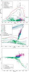 |
Fig. 8. Panels from top to bottom: EW(Li), log g, and γ as a function of Teff for the Li-rich giant (blue squares), (non-Li-rich) giant (fuchsia squares), and NG (green squares) outliers in the field of the young clusters, in all cases without taking into account the rest of field stars. Turquoise squares indicate potential NGs in the 1.01 > γ > 1.0 range. |
 |
Fig. 9. EW(Li)-versus-Teff and Kiel diagrams for the Li-rich giant (blue squares), (non-Li-rich) giant (fuchsia squares), and NG (green squares) outliers in the field of the intermediate-age and old clusters in the sample. |
5. Results: Cluster member selections
In this section we present our results from the membership analysis of each cluster, as summarised in Table 5. For each cluster, we report i the number of stars from the iDR4 sample observed with both UVES and GIRAFFE; (ii) those with measured values of EW(Li); (iii) the number of stars selected as candidate members; and (iv) the number of potential outlier contaminants. Readers are directed to the individual notes of Appendix A, where we offer a more detailed discussion of the membership analysis for each cluster, as well as commenting on features of interest regarding individual stars in the selection, and comparing our candidate lists with former membership studies (also listed in Table 1).
The full tables resulting from our membership analysis are provided in Appendix C. In the tables of Appendix C we show the results of our analysis and the final selections of candidate members for each of the 20 open clusters analysed, as well as the lists of giant and NG contaminants of interest also studied in this work. We indicate here for reference the columns for each table: The star ID, the GES object name from coordinates (CNAME), the RV of each star with its error, Teff with error, log g with error, γ index with error (for the young clusters), [Fe/H] metallicity with error, corrected values of EW(Li) with error, and flags for EW(Li) errors (see footnotes in the tables for more details). These are followed by the membership analysis columns, listing all candidates following all our criteria (RV, EW(Li), log g and/or γ index, [Fe/H]), as well as additional columns, whenever possible, listing candidates according to different studies from the literature. Each table ends with the list of final candidate members and non-members, as well as a final column listing the giant and NG contaminants with Li.
We also show our final selections in the following figures: Fig. 10 shows the EW(Li)-versus-Teff diagrams subdivided into young, intermediate-age, and old clusters; Fig. 11 shows the γ-versus-Teff diagram for the young clusters in our sample; and Fig. 12 shows the Kiel diagram for all clusters in the sample, for these same age ranges. Additionally, Appendix B shows all the individual figures for the pre-selected clusters, including both candidate member as well as giant and NG contaminants of interest.
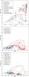 |
Fig. 10. EW(Li)-versus-Teff diagrams for the candidate members of the young clusters (1–50 Myr; top panel), as well as the intermediate-age (50–700 Myr; middle panel) and old clusters (> 700 Myr; bottom panel). Open squares indicate possible members only, while inverted triangles refer to Li-rich members. |
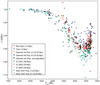 |
Fig. 11. Gravity index γ as a function of Teff for the young members in the young clusters of our sample. |
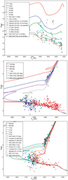 |
Fig. 12. Kiel diagrams for the candidate members of the young clusters (1–50 Myr; top panel), as well as the intermediate-age (50–700 Myr; middle panel) and old clusters (> 700 Myr; bottom panel). We overplot the PARSEC isochrones in a similar age range, with a metallicity of Z = 0.019. Open squares indicate possible members only, while inverted triangles refer to Li-rich members. |
6. Discussion
In Table 6 we show some further results of our membership analysis for the 20 clusters studied. As in Table 5, we show the number of stars in the field of each cluster from the initial iDR4 sample, and the number of candidate stars for all clusters, as well as the giant and NG outlier contaminants obtained as a parallel result during the membership analysis of each cluster. With these results we derived percentages of the candidate members and contaminants, which we used to assess the number of members and outliers found for different age ranges and clusters. Regarding the candidate members, these percentages are considered firstly with respect to all stars in the field of each cluster, and also with respect to all stars that present Li in the initial sample (as mentioned in Sect. 2, we also consider values from the OACT node for GIRAFFE stars in clusters older than 50 Myr). We consider, for each cluster, only percentages of any outlier class with respect to stars with EW(Li) > 10 mÅ, as explained in Sect. 4. However, in the case of the candidate members, percentages with respect to all stars with only EW(Li) > 10 mÅ are not considered given that there are, in the case of some of the older clusters, a series of attested members with Li values below this limit. We also note that the percentages of the giant contaminants only correspond to those stars with a EW(Li) value, given that for the giant outliers our selection is based more on A(Li) than on EW(Li) (see Sect. 4).
These percentages allow us to to rank the clusters and age ranges in terms of the percentage of candidate members and contaminants identified, with respect to all GES stars in the field of each cluster considered in this study. First considering all clusters, M67 is the cluster which has the highest percentage of candidate members (90%), followed by NGC 2516 (65%); then NGC 4815, Trumpler 20 and 23, and NGC 6802 (49–53%), NGC 6705 (48%), and Berkeley 44 (44%). Next we have Pismis 18 (38%), NGC 6005, and NGC 2547 (35%) (the young cluster with the highest percentage), Berkeley 81 (31%), and NGC 2243 and NGC 6633 (26–27%). So far, we see that, apart from NGC 2547, the clusters that provide the highest candidate percentages are either in the old or intermediate range. As to the remaining young clusters, γ Velorum (23%) and the SFRs are the ones with the highest percentages regarding the number of cluster candidates (ρ Oph with 19% and Cha I with 16%), followed by IC IC2391, IC 2602 and IC 4665, which are the clusters with the lowest percentages of cluster candidates in our list (2–9%).
Regarding age ranges separately, the lowest percentages for young clusters are found for IC 2391, IC 2602 and IC 4665, followed by the SFRs (ρ Oph and Cha I), γ Velorum, and NGC 2547, which presents the highest percentage. For intermediate clusters, NGC 6705 has the lowest member percentages, followed closely by NGC 4815, while NGC 2516 is the cluster for which we obtain the most members. In the case of the clusters in the old range, we note that M67 is the cluster with the highest percentage (90%), followed by Trumpler 23, NGC 6802, and Trumpler 20 and Berkeley 44 (44–53%); while the clusters with the lowest candidate percentages are Berkeley 81, NGC 6005, and Pismis 18 (31–38%), and NGC 6633 and NGC 2243 (26–27%).
Similarly, considering the outlier contaminants, we firstly note that we only obtained Li-rich contaminants in the field of 13 of the 20 clusters in our sample, and all percentages are low (1–3%) (as could be expected, considering that these stars only comprise 1–2% of FGK giants, as discussed in Sect. 4). Additionally, given that the selection criteria for giant outliers relies on A(Li) and not EW(Li), in the case of some clusters the Li-rich giants do not present Li values (or very few), and thus the percentages are listed as 0%. We find the highest percentages of Li-rich giants in the field of clusters Trumpler 23 and IC 2391 (3%), followed by 2% for Cha I, γ Vel, IC 2602, and NGC 6633. We find the lowest percentages in the field of ρ Oph, NGC 2547, and NGC 6005 (1%). We find Li-rich giants in all young clusters, with their presence becoming scarcer in the field of intermediate and old clusters. As for those giant outliers that are not Li-rich, which we listed for 18 of the 20 clusters in the sample (however, we again note that in some cases the percentages are negligible for lack of EW(Li) values), the highest percentages of these are found in the field of the young clusters: from 68–73% for IC 2391 and IC 2602, to 45–50% for Cha I and γ Vel, and 30–39% for the rest. We then find percentages in the 14–17% range for NGC 2516, NGC 6633, Trumpler 23, and NGC 6005; and the lowest percentages can be found in the field of NGC 6705, NGC 6802, and Pismis 18 (1–5%). Finally, regarding the NG contaminants (which we obtain for all 20 clusters of the sample), we find the highest percentages in the field of NGC 2243, Pismis 18, Berkeley 81, NGC 6005, and (IC 4665) (63–74%), followed by Berkeley 44, Trumpler 20 and NGC 6633 (50–56%), and the intermediate clusters NGC 6705 and NGC 4815 (43–49%). We then find percentages in the 20-40% range in the field of clusters such as NGC 6802, (ρ Oph), Trumpler 23, and (IC 2602). We find the lowest percentages (1–18%) for M67, NGC 2516, and young clusters such as Cha I or γ Vel. In the case of these NG outliers, we note that in Table 6 we list two percentages, the second one indicating that we take the stars in the 1.01 > γ > 1.0 range into account as well (see Sect. 4).
If we consider individual age ranges for the contaminant stars, we see that for young clusters the highest percentages for Li-rich and non-Li-rich giants are found in the fields of IC 2391 and IC 2602, followed by γ Vel and Cha I. On the other hand, the clusters with the lowest Li-rich giant percentages – such as IC 4665 and ρ Oph – seem to also present the highest percentages for NG contaminants. Regarding intermediate clusters, we find the highest percentage of non-Li-rich giants for NGC 2516, and we only find Li-rich giants in the field of NGC 6705, albeit with no EW(Li) values. We find similar percentages of NG outliers in the field of NGC 6705 and NGC 4815, with the lowest value for NGC 2516. We note that NGC 2516 is also the intermediate cluster with the highest member percentage, while NGC 4815 and NGC 6705 have the lowest member percentages (and the highest values for outlier contaminants). Finally, we only find Li-rich giants for five of the ten old clusters, with the clusters NGC 6633 and Trumpler 23 presenting the highest percentages. These two latter clusters, alongside NGC 6005, also present the highest percentages for non-Li-rich giant outliers. Regarding NG contaminants, we find the highest percentage in the field of cluster NGC 2243, closely followed by Berkeley 81, Pismis 18, and NGC 6005. We find the lowest values for M67, followed by NGC 6802, and Trumpler 23. We note that these clusters present both the highest member percentages and the lowest NG outlier values. This potential correlation of higher member percentages paired with lower contaminant percentages (especially the percentages for NG outliers) is something that we observe both in the intermediate and old age ranges, and to a lesser extent also for the young clusters.
7. Summary and future work
We used the GES-derived data provided in iDR4 to conduct an analysis of the membership and Li abundance of a series of 20 young, intermediate-age, and old clusters and associations ranging from 1 Myr to 5 Gyr.
We summarise our analysis and the main results of this work as follows:
-
During the membership selection process we used the iDR4 survey-derived radial velocities, stellar atmospheric parameters, lithium EWs, and metallicities to obtain lists of candidate members for the selected clusters.
-
We started using radial velocities to derive a series of initial RV candidates for each cluster. The position of these RV candidates in the EW(Li)-versus-Teff diagram then provided a series of lithium members. These members were analysed using gravity criteria (Kiel diagrams and the gravity index γ) that allow us to discard giant field contaminants. Finally, we used the [Fe/H] metallicity values to further confirm the membership of our candidates for each cluster. We also make use of recent studies based on Gaia DR1 and DR2 data to assess our candidate selections.
-
As a result of this membership study, we identified potential members for each cluster, as shown in Table 5 of this paper. The results of our membership analysis are discussed in more detail in the individual notes of Appendix A. Additionally, Appendix C presents the associated tables in which we also specify which membership criteria are fulfilled by each of the stars studied in all selected clusters.
-
Furthermore, as an additional result of our membership analysis we obtained a series of Li-rich giant and NG outliers with Li, which we aim to study in more detail. As in the case of the candidate members, the number of outliers for each cluster is also given in Table 5, and the list for each cluster is presented in Appendix C.
-
We find that our lists of cluster candidates agree with those of previous GES studies, when available. However, we also consider a series of candidate stars to be members despite not appearing in former lists, given that they fulfil all our membership criteria. We also note that we studied the membership of old cluster M67, which has not been previously studied using GES data.
Regarding our future work, we aim to calibrate the lithium–age relation and obtain its dependence on other stellar parameters derived from the GES spectroscopic observations, such as the level of chromospheric activity (Hα), accretion indicators, rotation (v sin i), metallicity ([Fe/H]), and other parameters available from the literature (e.g. photometric rotational period).
-
The age of each cluster will be revised using all this information, the lithium depletion boundary when possible, and other methods. For each cluster observed within GES, we also aim to include as part of our membership analysis all the EW(Li) measurements provided by other authors, as well as other well-known open clusters studied in the literature but not observed by GES. This will help to extend the age coverage.
-
We also aim to update the analysis and cluster member selections in the present study with the upgraded measurements and parameters of the last internal GES data release (iDR6), as well as astrometry from Gaia. This will also allow us to add new clusters to our calibration and therefore contribute to better constraining the lithium–age relation.
-
We plan to use these upgraded cluster candidate selections in a separate forthcoming paper in continuation of the work presented here in order to derive the lithium–age relation and its dependence on other stellar parameters. This will allow us to infer the ages of GES field stars whose age is still unknown, and to study the potential membership of these field stars to young associations and stellar kinematic groups of different ages.
-
Finally, another aspect of our future work involves studying in more detail some of the unknown non-member contaminants in the field of the clusters presented in this paper (Li-rich stars, and giant and NG outliers with Li), possibly including new young field stars or Li-rich giants.
And in fully convective stars the surface abundance of Li is rapidly depleted when the core reaches the Li-burning temperature.
In the end GES observed 65 clusters, as well as analysing ESO archive data for about 20 additional open clusters.
More details about how the recommended EWs were determined, as well as the associated errors, can be found in, e.g., Smiljanic et al. (2014), Lanzafame et al. (2015), and Tabernero et al. (2019).
The reason for excluding those clusters with high differential nebulosity from this study is the fact that the survey is fiber-fed, and thus subtraction of the nebular sky background is not a straightforward procedure (Bonito et al. 2013, 2020).
RStudio is an integrated development environment (IDE) for R, a programming language for statistical computing and graphics.
This tool shows the interquartile range (IQR) in a box-and-whisker plot, indicating the spread of the values in the distribution and the most probable outliers. The demarcation line for outliers is 1.5 × IQR – any value lying more than 1.5 times the length of the box from either end is considered to be a clear outlier of the distribution.
The 2σ clipping algorithm proceeds as follows: We fitted the distribution with a Gaussian curve to calculate its median (m) and standard deviation (σ). All points smaller or larger than m±2σ are then disregarded. This is repeated in an iterative manner until convergence is reached and the obtained σ remains within a certain tolerance level of the previous one. In each iteration, the range of input data decreases and so outliers can be effectively removed from the distribution.
In this study we discarded evolved stars in the field of young clusters without taking into account small effects, such as different initial accretion patterns which potentially lead to gravity spreads in this age range and thus to the possibility of biasing the sample to only objects with a particular accretion history.
For the Li membership analysis in this study we have generally not taken into account small Li variations and anomalies caused by a series of effects, such as planet engulfment or the influence of parameters such as chromospheric activity or rotation. These effects can also cause gravity spreads as well as variations on the metallicity in some cases. We plan on studying these effects and the dependence of Li on these stellar parameters in greater depth in our future work.
A tracer of accretion and youth indicator in young PMS stars, Hα10% refers to the width of the Hα emission line at 10% peak intensity. As already mentioned in Sect. 2 when discussing the cluster sample, Hα measurements are reliable only for clusters with no dominant nebular contribution to the emission.
As mentioned above, we relied less heavily on Cantat-Gaudin et al. (2018) from a comparative viewpoint because the study bases the membership analysis primarily on Gaia astrometry (parallaxes and proper motions as well as velocity) and does not use the spectroscopic information or lithium as main criteria, as we do in this study.
Acknowledgments
Financial support was provided by the Universidad Complutense de Madrid and by the Spanish Ministry of Economy and Competitiveness (MINECO) from project AYA2016-79425-C3-1-P. We acknowledge the support from INAF and Ministero dell’ Istruzione, dell’ Universitá’ e della Ricerca (MIUR) in the form of the grant “Premiale VLT 2012”. T.B. was funded by the project grant “The New Milky Way” from the Knut and Alice Wallenberg Foundation. J.I.G.H. acknowledges financial support from the Spanish Ministry of Science, Innovation and Universities (MICIU) under the 2003 Ramón y Cajal program RYC-2013-14875, and also from the Spanish Ministry project MICIU AYA2017-86389-P. E.M. acknowledges financial support from the Spanish Ministerio de Ciencia e Innovación through fellowship FPU15/01476. A.G. acknowledges support from the European Union FP7 programme from the UK space agency. U.H. acknowledges support from the Swedish National Space Agency (SNSA/Rymdstyrelsen). F.J.E. acknowledges financial support from the Spanish MINECO/FEDER through the grant AyA2017-84089. S.G.S acknowledges the support of Fundação para a Ciência e Tecnologia (FCT) through national funds and research grant (project ref. UID/FIS/04434/2013, and PTDC/FIS-AST/7073/2014). S.G.S also acknowledges the support from FCT through Investigador FCT contract of reference IF/00028/2014 and POPH/FSE (EC) by FEDER funding through the program “Programa Operacional de Factores de Competitividad” – COMPETE MT also acknowledges support from the FCT – Fundação para a Ciência e a Tecnologia through national funds (PTDC/FIS-AST/28953/2017) and by FEDER – Fundo Europeu de Desenvolvimento Regional through COMPETE2020 – Programa Operacional Competitividade e Internacionalização (POCI-01-0145-FEDER-028953). TM acknowledges support from the State Research Agency (AEI) of the Spanish Ministry of Science, Innovation and Universities (MCIU) and the European Regional Development Fund (FEDER) under grant AYA2017-88254-P Based on data products from observations made with ESO Telescopes at the La Silla Paranal Observatory under programme focusID 188.B-3002. These data products have been processed by the Cambridge Astronomy Survey Unit (CASU) at the Institute of Astronomy, University of Cambridge, and by the FLAMES/UVES reduction team at INAF–Osservatorio Astrofisico di Arcetri. These data have been obtained from the GES Data Archive, prepared and hosted by the Wide Field Astronomy Unit, Institute for Astronomy, University of Edinburgh, which is funded by the UK Science and Technology Facilities Council. This work was partly supported by the European Union FP7 programme through ERC grant number 320360 and by the Leverhulme Trust through grant RPG-2012-541. The results presented here benefit from discussions held during GES workshops and conferences supported by the ESF (European Science Foundation) through the GREAT Research Network Programme. This work was also supported by Fundação para a Ciência e Tecnologia (FCT) through the research grants UID/FIS/04434/2019, UIDB/04434/2020 and UIDP/04434/2020. This work has made use of data from the European Space Agency (ESA) mission Gaia (https://www.cosmos.esa.int/gaia), processed by the Gaia Data Processing and Analysis Consortium (DPAC, https://www.cosmos.esa.int/web/gaia/dpac/consortium). Funding for the DPAC has been provided by national institutions, in particular the institutions participating in the Gaia Multilateral Agreement. This publication makes use of the VizieR database (Ochsenbein et al. 2000) and the SIMBAD database (Wenger et al. 2000), both operated at CDS, Centre de Données astronomiques de Strasbourg, France. This research also made use of the WEBDA database, operated at the Department of Theoretical Physics and Astrophysics of the Masaryk University, and the interactive graphical viewer and editor for tabular data TOPCAT (Taylor 2005). For the analysis of the distributions of RV and metallicity we used RStudio Team (2015). Integrated Development for R. RStudio, Inc., Boston, MA (http://www.rstudio.com/). Finally, we would like to thank the anonymous referee for helpful comments and suggestions.
References
- Bailey, J. I., Mateo, M., White, R. J., Shectman, S. A., & Crane, J. D. 2018, MNRAS, 475, 1609 [NASA ADS] [CrossRef] [Google Scholar]
- Balachandran, S. 1995, ApJ, 446, 203 [NASA ADS] [CrossRef] [Google Scholar]
- Barrado y Navascués, D., Stauffer, J. R., & Patten, B. M. 1999, ApJ, 522, L53 [NASA ADS] [CrossRef] [Google Scholar]
- Barrado y Navascués, D., Stauffer, J. R., Briceño, C., et al. 2001, ApJS, 134, 103 [NASA ADS] [CrossRef] [Google Scholar]
- Barrado y Navascués, D., Stauffer, J. R., & Jayawardhana, R. 2004, ApJ, 614, 386 [NASA ADS] [CrossRef] [Google Scholar]
- Beccari, G., Boffin, H. M. J., Jerabkova, T., et al. 2018, MNRAS, 481, L11 [NASA ADS] [CrossRef] [Google Scholar]
- Bergemann, M., Ruchti, G. R., Serenelli, A., et al. 2014, A&A, 565, A89 [NASA ADS] [CrossRef] [EDP Sciences] [Google Scholar]
- Bonito, R., Prisinzano, L., Guarcello, M. G., & Micela, G. 2013, A&A, 556, A108 [NASA ADS] [CrossRef] [EDP Sciences] [Google Scholar]
- Bonito, R., Prisinzano, L., Venuti, F., et al. 2020, A&A, 642, A56 [CrossRef] [EDP Sciences] [Google Scholar]
- Bossini, D., Vallenari, A., Bragaglia, A., et al. 2019, A&A, 623, A108 [NASA ADS] [CrossRef] [EDP Sciences] [Google Scholar]
- Bouvier, J. 2008, A&A, 489, L53 [NASA ADS] [CrossRef] [EDP Sciences] [Google Scholar]
- Bouvier, J., Lanzafame, A. C., Venuti, L., et al. 2016, A&A, 590, A78 [NASA ADS] [CrossRef] [EDP Sciences] [Google Scholar]
- Bravi, L., Zari, E., Sacco, G. G., et al. 2018, A&A, 615, A37 [NASA ADS] [CrossRef] [EDP Sciences] [Google Scholar]
- Bressan, A., Marigo, P., Girardi, L., et al. 2012, MNRAS, 427, 127 [NASA ADS] [CrossRef] [Google Scholar]
- Brucalassi, A., Koppenhoefer, J., Saglia, R., et al. 2017, A&A, 603, A85 [NASA ADS] [CrossRef] [EDP Sciences] [Google Scholar]
- Cameron, A. G. W., & Fowler, W. A. 1971, ApJ, 164, 111 [Google Scholar]
- Cánovas, H., Cantero, C., Cieza, L., et al. 2019, A&A, 626, A80 [NASA ADS] [CrossRef] [EDP Sciences] [Google Scholar]
- Cantat-Gaudin, T., Vallenari, A., Zaggia, S., et al. 2014, A&A, 569, A17 [NASA ADS] [CrossRef] [EDP Sciences] [Google Scholar]
- Cantat-Gaudin, T., Jordi, C., Vallenari, A., et al. 2018, A&A, 618, A93 [NASA ADS] [CrossRef] [EDP Sciences] [Google Scholar]
- Carlberg, J. K. 2014, AJ, 147, 138 [NASA ADS] [CrossRef] [Google Scholar]
- Casali, G., Magrini, L., Tognelli, E., et al. 2019, A&A, 629, A62 [CrossRef] [EDP Sciences] [Google Scholar]
- Casey, A. R., Ruchti, G., Masseron, T., et al. 2016, MNRAS, 461, 3336 [NASA ADS] [CrossRef] [Google Scholar]
- Castro, M., Duarte, T., Pace, G., & do Nascimento, J.-D. 2016, A&A, 590, A94 [NASA ADS] [CrossRef] [EDP Sciences] [Google Scholar]
- Charbonnel, C., & Talon, S. 2005, Science, 309, 2189 [Google Scholar]
- Damiani, F., Prisinzano, L., Micela, G., et al. 2014, A&A, 566, A50 [NASA ADS] [CrossRef] [EDP Sciences] [Google Scholar]
- Delgado Mena, E., Tsantaki, M., Sousa, S. G., et al. 2016, A&A, 587, A66 [NASA ADS] [CrossRef] [EDP Sciences] [Google Scholar]
- Deliyannis, C. P., Demarque, P., & Pinsonneault, M. H. 1990, BAAS, 22, 1214 [Google Scholar]
- De Silva, G. M., D’Orazi, V., Melo, C., et al. 2013, MNRAS, 431, 1005 [NASA ADS] [CrossRef] [Google Scholar]
- Dias, W. S., Alessi, B. S., Moitinho, A., & Lépine, J. R. D. 2002, A&A, 389, 871 [NASA ADS] [CrossRef] [EDP Sciences] [Google Scholar]
- Donati, P., Beccari, G., Bragaglia, A., Cignoni, M., & Tosi, M. 2014a, MNRAS, 437, 1241 [NASA ADS] [CrossRef] [Google Scholar]
- Donati, P., Cantat Gaudin, T., Bragaglia, A., et al. 2014b, A&A, 561, A94 [NASA ADS] [CrossRef] [EDP Sciences] [Google Scholar]
- Duncan, D. K. 1981, ApJ, 248, 651 [NASA ADS] [CrossRef] [Google Scholar]
- Elliott, P., Huélamo, N., Bouy, H., et al. 2015, A&A, 580, A88 [NASA ADS] [CrossRef] [EDP Sciences] [Google Scholar]
- Franciosini, E., Sacco, G. G., Jeffries, R. D., et al. 2018, A&A, 616, L12 [NASA ADS] [CrossRef] [EDP Sciences] [Google Scholar]
- Frasca, A., Biazzo, K., Lanzafame, A. C., et al. 2015, A&A, 575, A4 [NASA ADS] [CrossRef] [EDP Sciences] [Google Scholar]
- Friel, E. D. 1995, ARA&A, 33, 381 [NASA ADS] [CrossRef] [Google Scholar]
- Friel, E. D., & Janes, K. A. 1993, A&A, 267, 75 [NASA ADS] [Google Scholar]
- Friel, E. D., Jacobson, H. R., & Pilachowski, C. A. 2010, AJ, 139, 1942 [NASA ADS] [CrossRef] [Google Scholar]
- Friel, E. D., Donati, P., Bragaglia, A., et al. 2014, A&A, 563, A117 [NASA ADS] [CrossRef] [EDP Sciences] [Google Scholar]
- Gaia Collaboration (Brown, A. G. A., et al.) 2018, A&A, 616, A1 [NASA ADS] [CrossRef] [EDP Sciences] [Google Scholar]
- Gao, Q., Shi, J.-R., Yan, H.-L., et al. 2019, ApJS, 245, 33 [CrossRef] [Google Scholar]
- Geller, A. M., Latham, D. W., & Mathieu, R. D. 2015, AJ, 150, 97 [NASA ADS] [CrossRef] [Google Scholar]
- Gilmore, G., Randich, S., Asplund, M., et al. 2012, The Messenger, 147, 25 [NASA ADS] [Google Scholar]
- Hatzidimitriou, D., Held, E. V., Tognelli, E., et al. 2019, A&A, 626, A90 [NASA ADS] [CrossRef] [EDP Sciences] [Google Scholar]
- Hayes, C. R., & Friel, E. D. 2014, AJ, 147, 69 [NASA ADS] [CrossRef] [Google Scholar]
- Heiter, U., Soubiran, C., Netopil, M., & Paunzen, E. 2014, A&A, 561, A93 [NASA ADS] [CrossRef] [EDP Sciences] [Google Scholar]
- Hobbs, L. M., & Pilachowski, C. 1986, ApJ, 311, L37 [NASA ADS] [CrossRef] [Google Scholar]
- Iben, I. 1967, ApJ, 147, 624 [NASA ADS] [CrossRef] [Google Scholar]
- Irwin, J., Hodgkin, S., Aigrain, S., et al. 2007, MNRAS, 377, 741 [NASA ADS] [CrossRef] [Google Scholar]
- Jackson, R. J., & Jeffries, R. D. 2010, MNRAS, 407, 465 [NASA ADS] [CrossRef] [Google Scholar]
- Jackson, R. J., Jeffries, R. D., Randich, S., et al. 2016, A&A, 586, A52 [NASA ADS] [CrossRef] [EDP Sciences] [Google Scholar]
- Jacobson, H. R., Friel, E. D., & Pilachowski, C. A. 2011, AJ, 141, 58 [NASA ADS] [CrossRef] [Google Scholar]
- Jacobson, H. R., Friel, E. D., Jílková, L., et al. 2016, A&A, 591, A37 [NASA ADS] [CrossRef] [EDP Sciences] [Google Scholar]
- Jeffries, R. D. 1997, MNRAS, 292, 177 [NASA ADS] [CrossRef] [Google Scholar]
- Jeffries, R. D., James, D. J., & Thurston, M. R. 1998, MNRAS, 300, 550 [NASA ADS] [CrossRef] [Google Scholar]
- Jeffries, R. D., Thurston, M. R., & Hambly, N. C. 2001, A&A, 375, 863 [NASA ADS] [CrossRef] [EDP Sciences] [Google Scholar]
- Jeffries, R. D., Totten, E. J., Harmer, S., & Deliyannis, C. P. 2002, MNRAS, 336, 1109 [NASA ADS] [CrossRef] [Google Scholar]
- Jeffries, R. D., Jackson, R. J., James, D. J., & Cargile, P. A. 2009, MNRAS, 400, 317 [NASA ADS] [CrossRef] [Google Scholar]
- Jeffries, R. D., Jackson, R. J., Cottaar, M., et al. 2014, A&A, 563, A94 [NASA ADS] [CrossRef] [EDP Sciences] [Google Scholar]
- Jones, B. F., Fischer, D., & Soderblom, D. R. 1999, AJ, 117, 330 [NASA ADS] [CrossRef] [Google Scholar]
- Kang, W., & Lee, S.-G. 2012, MNRAS, 425, 3162 [Google Scholar]
- Kharchenko, N. V., Piskunov, A. E., Röser, S., Schilbach, E., & Scholz, R.-D. 2005, A&A, 438, 1163 [NASA ADS] [CrossRef] [EDP Sciences] [MathSciNet] [Google Scholar]
- Lanzafame, A. C., Frasca, A., Damiani, F., et al. 2015, A&A, 576, A80 [NASA ADS] [CrossRef] [EDP Sciences] [Google Scholar]
- Lagarde, N., Decressin, T., Charbonnel, C., et al. 2012, A&A, 543, A108 [NASA ADS] [CrossRef] [EDP Sciences] [Google Scholar]
- López Martí, B., Jiménez-Esteban, F., Bayo, A., et al. 2013, A&A, 556, A144 [NASA ADS] [CrossRef] [EDP Sciences] [Google Scholar]
- Lyubimkov, L. S. 2016, Astrophysics, 59, 411 [NASA ADS] [CrossRef] [Google Scholar]
- Magrini, L., Randich, S., Romano, D., et al. 2014, A&A, 563, A44 [NASA ADS] [CrossRef] [EDP Sciences] [Google Scholar]
- Magrini, L., Randich, S., Donati, P., et al. 2015, A&A, 580, A85 [NASA ADS] [CrossRef] [EDP Sciences] [Google Scholar]
- Magrini, L., Randich, S., Kordopatis, G., et al. 2017, A&A, 603, A2 [NASA ADS] [CrossRef] [EDP Sciences] [Google Scholar]
- Magrini, L., Vincenzo, F., Randich, S., et al. 2018, A&A, 618, A102 [NASA ADS] [CrossRef] [EDP Sciences] [Google Scholar]
- Marsden, S. C., Carter, B. D., & Donati, J.-F. 2009, MNRAS, 399, 888 [NASA ADS] [CrossRef] [Google Scholar]
- Martin, E. L., & Montes, D. 1997, A&A, 318, 805 [Google Scholar]
- Martín, E. L., Lodieu, N., Pavlenko, Y., & Béjar, V. J. S. 2018, ApJ, 856, 40 [NASA ADS] [CrossRef] [Google Scholar]
- Merle, T., Van Eck, S., Jorissen, A., et al. 2017, A&A, 608, A95 [NASA ADS] [CrossRef] [EDP Sciences] [Google Scholar]
- Merle, T., Van der Swaelmen, M., Van Eck, S., et al. 2020, A&A, 635, A155 [Google Scholar]
- Messina, S., Parihar, P., Koo, J.-R., et al. 2010, A&A, 513, A29 [NASA ADS] [CrossRef] [EDP Sciences] [Google Scholar]
- Messina, S., Desidera, S., Lanzafame, A. C., Turatto, M., & Guinan, E. F. 2011, A&A, 532, A10 [NASA ADS] [CrossRef] [EDP Sciences] [Google Scholar]
- Montes, D., López-Santiago, J., Fernández-Figueroa, M. J., & Gálvez, M. C. 2001, A&A, 379, 976 [NASA ADS] [CrossRef] [EDP Sciences] [Google Scholar]
- Netopil, M., Paunzen, E., Heiter, U., & Soubiran, C. 2016, A&A, 585, A150 [NASA ADS] [CrossRef] [EDP Sciences] [Google Scholar]
- Neuhaeuser, R., Torres, G., Sterzik, M. F., & Randich, S. 1997, A&A, 325, 647 [Google Scholar]
- Ochsenbein, F., Bauer, P., & Marcout, J. 2000, A&AS, 143, 23 [NASA ADS] [CrossRef] [EDP Sciences] [Google Scholar]
- Oliveira, J. M., Jeffries, R. D., Devey, C. R., et al. 2003, MNRAS, 342, 651 [NASA ADS] [CrossRef] [Google Scholar]
- Overbeek, J. C., Friel, E. D., & Jacobson, H. R. 2016, ApJ, 824, 75 [NASA ADS] [CrossRef] [Google Scholar]
- Overbeek, J. C., Friel, E. D., Donati, P., et al. 2017, A&A, 598, A68 [NASA ADS] [CrossRef] [EDP Sciences] [Google Scholar]
- Pace, G., Castro, M., Meléndez, J., Théado, S., & do Nascimento, J.-D., Jr 2012, A&A, 541, A150 [NASA ADS] [CrossRef] [EDP Sciences] [Google Scholar]
- Pallavicini, R., Pasquini, L., & Randich, S. 1997, Mem. Soc. Astron. Ital., 68, 933 [Google Scholar]
- Pallavicini, R., Randich, S., & Sestito, P. 2005, in 13th Cambridge Workshop on Cool Stars, Stellar Systems and the Sun, 560, 867 [Google Scholar]
- Pancino, E., Lardo, C., Altavilla, G., et al. 2017, A&A, 598, A5 [NASA ADS] [CrossRef] [EDP Sciences] [Google Scholar]
- Pasquini, L., Randich, S., & Pallavicini, R. 1997, A&A, 325, 535 [NASA ADS] [Google Scholar]
- Pasquini, L., Avila, G., Blecha, A., et al. 2002, The Messenger, 110, 1 [Google Scholar]
- Pasquini, L., Brucalassi, A., Ruiz, M. T., et al. 2012, A&A, 545, A139 [NASA ADS] [CrossRef] [EDP Sciences] [Google Scholar]
- Patten, B. M., & Simon, T. 1996, ApJS, 106, 489 [NASA ADS] [CrossRef] [Google Scholar]
- Peña, J. H., Robleto-Orús, A., Piña, D. S., et al. 2017, Rev. Mex. Astron. Astrofis., 53, 309 [Google Scholar]
- Piatti, A. E., Clariá, J. J., Bica, E., Geisler, D., & Minniti, D. 1998, AJ, 116, 801 [NASA ADS] [CrossRef] [Google Scholar]
- Platais, I., Melo, C., Mermilliod, J.-C., et al. 2007, A&A, 461, 509 [NASA ADS] [CrossRef] [EDP Sciences] [Google Scholar]
- Postnikova, E. S., Chupina, N. V., & Vereshchagin, S. V. 2019, INASAN Sci. Rep., 3, 336 [Google Scholar]
- Postnikova, E. S., Elsanhoury, W. H., Sariya, D. P., et al. 2020, Res. Astron. Astrophys., 20, 016 [CrossRef] [Google Scholar]
- Prisinzano, L., Damiani, F., Micela, G., et al. 2016, A&A, 589, A70 [NASA ADS] [CrossRef] [EDP Sciences] [Google Scholar]
- Randich, S., Aharpour, N., Pallavicini, R., Prosser, C. F., & Stauffer, J. R. 1997, A&A, 323, 86 [NASA ADS] [Google Scholar]
- Randich, S., Pallavicini, R., Meola, G., Stauffer, J. R., & Balachandran, S. C. 2001, A&A, 372, 862 [NASA ADS] [CrossRef] [EDP Sciences] [Google Scholar]
- Randich, S., Primas, F., Pasquini, L., & Pallavicini, R. 2002, A&A, 387, 222 [NASA ADS] [CrossRef] [EDP Sciences] [Google Scholar]
- Randich, S., Gilmore, G., & Gaia-ESO Consortium 2013, The Messenger, 154, 47 [NASA ADS] [Google Scholar]
- Randich, S., Tognelli, E., Jackson, R., et al. 2018, A&A, 612, A99 [NASA ADS] [CrossRef] [EDP Sciences] [Google Scholar]
- Richer, H. B., Fahlman, G. G., Rosvick, J., & Ibata, R. 1998, ApJ, 504, L91 [NASA ADS] [CrossRef] [Google Scholar]
- Rigliaco, E., Wilking, B., Meyer, M. R., et al. 2016, A&A, 588, A123 [NASA ADS] [CrossRef] [EDP Sciences] [Google Scholar]
- Robrade, J., & Schmitt, J. H. M. M. 2007, A&A, 461, 669 [NASA ADS] [CrossRef] [EDP Sciences] [Google Scholar]
- Roccatagliata, V., Sacco, G. G., Franciosini, E., & Randich, S. 2018, A&A, 617, L4 [NASA ADS] [CrossRef] [EDP Sciences] [Google Scholar]
- Sacco, G. G., Jeffries, R. D., Randich, S., et al. 2015, A&A, 574, L7 [NASA ADS] [CrossRef] [EDP Sciences] [Google Scholar]
- Sacco, G. G., Spina, L., Randich, S., et al. 2017, A&A, 601, A97 [NASA ADS] [CrossRef] [EDP Sciences] [Google Scholar]
- Sampedro, L., Dias, W. S., Alfaro, E. J., Monteiro, H., & Molino, A. 2017, MNRAS, 470, 3937 [NASA ADS] [CrossRef] [Google Scholar]
- Sestito, P., & Randich, S. 2005, A&A, 442, 615 [NASA ADS] [CrossRef] [EDP Sciences] [Google Scholar]
- Siess, L., Dufour, E., & Forestini, M. 2000, A&A, 358, 593 [Google Scholar]
- Smiljanic, R., Randich, S., & Pasquini, L. 2011, A&A, 535, A75 [NASA ADS] [CrossRef] [EDP Sciences] [Google Scholar]
- Smiljanic, R., Korn, A. J., Bergemann, M., et al. 2014, A&A, 570, A122 [NASA ADS] [CrossRef] [EDP Sciences] [Google Scholar]
- Smiljanic, R., Franciosini, E., Randich, S., et al. 2016, A&A, 591, A62 [NASA ADS] [CrossRef] [EDP Sciences] [Google Scholar]
- Smiljanic, R., Franciosini, E., Bragaglia, A., et al. 2018, A&A, 617, A4 [NASA ADS] [CrossRef] [EDP Sciences] [Google Scholar]
- Smith, V. V., Plez, B., Lambert, D. L., & Lubowich, D. A. 1995, ApJ, 441, 735 [NASA ADS] [CrossRef] [Google Scholar]
- Sneden, C. A. 1973, Ph.D. Thesis, Univ. Texas at Austin, USA [Google Scholar]
- Soderblom, D. R. 1983, ApJS, 53, 1 [NASA ADS] [CrossRef] [Google Scholar]
- Soderblom, D. R. 2010, ARA&A, 48, 581 [NASA ADS] [CrossRef] [Google Scholar]
- Soderblom, D. R., Oey, M. S., Johnson, D. R. H., & Stone, R. P. S. 1990, AJ, 99, 595 [NASA ADS] [CrossRef] [Google Scholar]
- Soderblom, D. R., Jones, B. F., Balachandran, S., et al. 1993, AJ, 106, 1059 [NASA ADS] [CrossRef] [Google Scholar]
- Soderblom, D. R., Jones, B. F., Stauffer, J. R., & Chaboyer, B. 1995, AJ, 110, 729 [NASA ADS] [CrossRef] [Google Scholar]
- Soderblom, D. R., Hillenbrand, L. A., Jeffries, R. D., Mamajek, E. E., & Naylor, T. 2014, Protostars Planets VI, 3, 219 [Google Scholar]
- Soubiran, C., Cantat-Gaudin, T., Romero-Gómez, M., et al. 2018, A&A, 619, A155 [NASA ADS] [CrossRef] [EDP Sciences] [Google Scholar]
- Spezzi, L., Pagano, I., Marino, G., et al. 2009, A&A, 499, 541 [NASA ADS] [CrossRef] [EDP Sciences] [Google Scholar]
- Spina, L., Randich, S., Palla, F., et al. 2014a, A&A, 568, A2 [NASA ADS] [CrossRef] [EDP Sciences] [Google Scholar]
- Spina, L., Randich, S., Palla, F., et al. 2014b, A&A, 567, A55 [NASA ADS] [CrossRef] [EDP Sciences] [Google Scholar]
- Spina, L., Randich, S., Magrini, L., et al. 2017, A&A, 601, A70 [NASA ADS] [CrossRef] [EDP Sciences] [Google Scholar]
- Stauffer, J. R., Hartmann, L. W., Prosser, C. F., et al. 1997, ApJ, 479, 776 [NASA ADS] [CrossRef] [Google Scholar]
- Tabernero, H. M., Marfil, E., Montes, D., et al. 2019, A&A, 628, A131 [CrossRef] [EDP Sciences] [Google Scholar]
- Tang, B., Geisler, D., Friel, E., et al. 2017, A&A, 601, A56 [NASA ADS] [CrossRef] [EDP Sciences] [Google Scholar]
- Tautvaišienė, G., Drazdauskas, A., Mikolaitis, Š., et al. 2015, A&A, 573, A55 [NASA ADS] [CrossRef] [EDP Sciences] [Google Scholar]
- Taylor, M. B. 2005, Astron. Data Anal. Softw. Syst. XIV, 347, 29 [Google Scholar]
- Terndrup, D. M., Pinsonneault, M., Jeffries, R. D., et al. 2002, ApJ, 576, 950 [NASA ADS] [CrossRef] [Google Scholar]
- Umezu, M., & Saio, H. 2000, MNRAS, 316, 307 [NASA ADS] [CrossRef] [Google Scholar]
- Ventura, P., Zeppieri, A., Mazzitelli, I., & D’Antona, F. 1998, A&A, 331, 1011 [NASA ADS] [Google Scholar]
- Vereshchagin, S. V., Tutukov, A. V., & Chupina, N. V. 2019, INASAN Sci. Rep., 3, 302 [Google Scholar]
- Wenger, M., Ochsenbein, F., Egret, D., et al. 2000, A&AS, 143, 9 [NASA ADS] [CrossRef] [EDP Sciences] [Google Scholar]
- White, R. J., & Basri, G. 2003, ApJ, 582, 1109 [NASA ADS] [CrossRef] [Google Scholar]
Appendix A: Individual cluster notes
A.1. SFRs (age ≤ 5 Myr) and young open clusters (age ≤ 50 Myr)
A.1.1. ρ Ophiuchi
Of the final members in ρ Oph, 29 belong to the SFR L1688 (Rigliaco et al. 2016), and 17 of them are also strong accretors with Hα10% > 270–300 km s−1. Of these 17 accreting stars, only one (J16273311−2441152) does not pass our gravity criteria. This star, with γ = 1.026 and A(Li) = 3.18, could be listed as a potential Li-rich giant, but due to the fact that it is also a strong accretor (with Hα10% = 456 km s−1)we counted it as a likely member of ρ Oph, also in accordance with Rigliaco et al. (2016). Cánovas et al. (2019) listed 38 candidates that are common to our selection (for the remaining two stars in their study the iDR4 sample does not include Li measurements). We note that one of the stars in our final selection (J16270456−2442140) presents a [Fe/H] value which deviates appreciably from the rest of candidates, while another four candidates are RV non-members with RVs deviating 2.5σ (or 5 km s−1) from the mean of the cluster and in one case up to 4σ (or 8 km s−1). We included these stars given that they fulfil the rest of the membership criteria (especially regarding gravity indicators and lithium), and they are also listed as candidates by studies such as Cánovas et al. (2019).
A.1.2. Chamaeleon I
As a result of the analysis of Cha I we find 35 accreting stars, of which only one (J11092578−7623207) is not a Li member. This is probably due to possible veiling suppressing the absorption Li line, and so we classified this strong accretor as an additional likely member. We also note that three of the stars in our final selection are RV non-members, with RVs deviating 2.7–4σ (or 4–6 km s−1) from the mean of the cluster and, in one case, up to 6.7σ (or 10 km s−1). These stars fulfil the rest of the membership criteria (especially regarding gravity indicators and lithium), and they are also listed as candidates by Sacco et al. (2017) and Robrade & Schmitt (2007). Regarding previous selections, we find all the UVES members observed by Spina et al. (2014a) in our selection, except for J10555973−7724399 and J11092378−7623207, for which several parameters are not released in the iDR4 catalog. On the other hand, all our candidate stars are included in the member list of Sacco et al. (2017), except for one (J11110238−7613327), which is listed in Robrade & Schmitt (2007). Regarding field contaminants, one Li-rich giant (J11000515−7623259) is listed in Casey et al. (2016).
A.1.3. Vela OB2 association: γ Velorum and NGC 2547
The cluster membership selections for both of these clusters consist of 210 stars in γ Vel (104 in γ Vel A and 83 in γ Vel B, as well as 23 additional candidate stars that are not associated to a specific population), and 107 stars in NGC 2547 (88 in NGC 2547 A and 19 in NGC 2547 B). As mentioned in Sect. 3, for this study we used the membership selections obtained by a series of former studies in the literature: Regarding γ Vel, we first used Jeffries et al. (2014), the study specifying the members of Pop. A and B, as well as a series of other GES studies (Damiani et al. 2014; Spina et al. 2014b; Frasca et al. 2015; Prisinzano et al. 2016). For NGC 2547 we used Sacco et al. (2015), together with the Gaia studies conducted by Cantat-Gaudin et al. (2018) and Randich et al. (2018). All three of these latter papers list the membership probabilities of each candidate to Pop. A/B. For γ Vel, we find 23 additional candidates that were not listed in the previous GES studies. We added them to the candidates not associated with one of the two γ Vel populations. We note that Frasca et al. (2015) used the data from Jeffries et al. (2014), and in this case we consider five stars listed as members which had no listed Pop. A/B in Jeffries et al. (2014).
Recent studies Cantat-Gaudin et al. (2018) and Randich et al. (2018) furthermore offer updated membership probabilities for NGC 2547 (as well as a series of other clusters in our sample), using data from Gaia. Randich et al. (2018) listed a series of new members with respect to Sacco et al. (2015). Although their membership probabilities for each population are generally consistent with each other, six stars were associated with different populations in Sacco et al. (2015) and Randich et al. (2018). In this case, we adopted the membership from Randich et al. (2018), as this is the most recent study which used both the GES iDR4 data and Gaia DR2 data. For this cluster we also compared the member stars in Sacco et al. (2015), Cantat-Gaudin et al. (2018) and Randich et al. (2018) with the candidate members in Bravi et al. (2018). For all our candidates, Bravi et al. (2018) find high probabilities, namely ranging from 60 to 100%, of being RV members of the cluster.
Finally, as to field contaminants, we also find two of the γ Vel Li-rich giants in our list (J08095783−4701385 and J08102116−4740125), as well as one of the Li-rich giants from NGC 2547 (J08110403−4852137), in Casey et al. (2016). Another one, (J08110403−4658057) in γ Vel, is listed in Smiljanic et al. (2018). Regarding the NG non-members, we included only the contaminants marked as such by the aforementioned studies. The reason for this is that without an additional membership analysis (as we have done for the rest of the clusters) we cannot confirm many NG stars not listed by these studies as either members or contaminants.
A.1.4. IC 2391
We discarded but 34 Li members of IC 2391 for not having any measured values of chromospheric activity, taking into account both the accretion and chromospheric EW(Hα). From these 34 stars, we discarded seven as non-members for not fulfilling our RV and metallicity criteria. Some of them have very large RVs deviating up to 150σ (or 450 km s−1) from the mean of the cluster. Four of these seven stars are also listed as non-members by Randich et al. (2018). We also note that we consider three candidates which are RV non-members, with RVs deviating from the mean by up to 4.3σ (or 13 km s−1), as they are good spectroscopic candidates, fulfilling the rest of the membership criteria (especially regarding gravity indicators and lithium).
We first compared our selection with a series of non-GES studies, finding ten of our candidates in one or more previous lists (Patten & Simon 1996; Barrado y Navascués et al. 2001, 2004; Platais et al. 2007; Marsden et al. 2009; Spezzi et al. 2009; Messina et al. 2011; De Silva et al. 2013; Elliott et al. 2015). Regarding GES studies, Bravi et al. (2018) derived RV membership probabilities and lists of candidate members for this cluster (alongside IC 2602, IC 4665 and NGC 2547) using iDR4 data, which were selected from their EW(Li), gravity, and metallicity values reported in the GES iDR4 data. Comparing our final selection of 27 members with the list of 53 candidate stars of Bravi et al. (2018), we find 30 kinematic candidates and 17 final members in common (all of the common members stars have high RV membership probabilities of at least 0.95, except for two stars in the 0.7–0.9 range). We note that, for many stars Bravi et al. (2018) used values of EW(Li) and/or Teff which were derived from one of the WG12 nodes and do not appear in the iDR4 sample. As a result, we excluded these stars from our membership analysis and only consider those stars in Bravi et al. (2018) with EW(Li) values in the iDR4 sample. Our mean RV and σ for IC 2391 also agree with the estimates in Bravi et al. (2018).
Finally, Cantat-Gaudin et al. (2018) and Randich et al. (2018) also list updated membership probabilities for IC 2391. We have 19 common stars listed as members with Randich et al. (2018), as well as 13 stars with Cantat-Gaudin et al. (2018). As we mention in Sect. 3.5, in this study we relied more heavily on Randich et al. (2018), as they used the same iDR4 sample and their membership criteria are similar to ours. We relied less heavily on Cantat-Gaudin et al. (2018) from a comparative standpoint, given that they primarily base their membership analysis on Gaia astrometry and do not use spectroscopic criteria. We note that we discarded a small number of possible candidate stars which were listed as non-members by both Randich et al. (2018) and Bravi et al. (2018), and we also did not consider a small number of stars listed by Randich et al. (2018) and Cantat-Gaudin et al. (2018) for not having a measured Hα in the iDR4 sample (the latter also applies to the clusters IC 2602 and IC 4665 listed below). We also mention here a series of recent studies that used Gaia-DR2 data to study the spacial-kinematic distribution and cluster membership of IC 2391 (Postnikova et al. 2019, 2020; Vereshchagin et al. 2019).
A.1.5. IC 2602
We discarded all but 42 of the 52 Li candidates in IC 2602 for not having measured values of chromospheric activity. Of these 42 Li members we finally discarded ten stars, all of which are also listed as non-members by Randich et al. (2018) and Bravi et al. (2018). Comparing our selection with former studies, we find four of our candidates in one or more of the member lists of these non-GES studies (Randich et al. 1997, 2001; Stauffer et al. 1997; Marsden et al. 2009; Smiljanic et al. 2011). Regarding GES studies, we find 55 kinematic candidates and 27 final members in common with the list of 101 candidates in Bravi et al. (2018). As in the case of IC 2391, many of the stars in Bravi et al. (2018) have no EW(Li) values in the iDR4 sample, and therefore we excluded them in our own membership analysis. The mean RV and σ derived in Bravi et al. (2018) for IC 2602 are also in agreement with the ones obtained in this paper. As for Gaia studies, we have 28 common stars listed as members with Randich et al. (2018), as well as 19 stars with Cantat-Gaudin et al. (2018).
A.1.6. IC 4665
We discarded all but 51 Li members in IC 4665 for not having measured values of EW(Hα) in the GES sample, and finally discarded 11 of these 51 stars as non-members for not fulfilling our RV and metallicity criteria. Five of these stars are also listed as non-members by both Randich et al. (2018) and Bravi et al. (2018). Finally, three of the final Li members are also listed as non-members by Randich et al. (2018), and therefore we decided to consider them as possible candidates only. Comparing our selection with former studies, we find six of our member stars in Jeffries et al. (2009). Regarding GES studies, we find 30 kinematic candidates and 19 final members in common with the list of 122 candidates in Bravi et al. (2018). Our mean RV and σ are also consistent with the previous estimates in this work. As for Gaia, we find 21 common stars listed as members with both Randich et al. (2018) and Cantat-Gaudin et al. (2018).
A.2. Intermediate-age clusters (age = 50–700 Myr)
A.2.1. NGC 2516
In our selection of candidate members of NGC 2516 we listed 30 Li members with RVs deviating up to 13σ (or 8 km s−1) from the mean of the cluster. All of these stars fulfil our main criteria and are also included as members by Randich et al. (2018). Regarding all the intermediate clusters of our sample, as already mentioned in Sects. 3.2 and 3.4, we also note that, given the lower resolution of the GIRAFFE spectra, we accepted as candidates a number of Li members with [Fe/H] values outside the limit of 2σ from the cluster mean provided by our fit.
Comparing our UVES selection with existing GES studies, we find all of our final UVES candidates to be the same as those in the list of NGC 2516 stars classified as members by Jacobson et al. (2016), and all but two of our candidates are also listed as members by Magrini et al. (2017). Regarding the GIRAFFE candidates, we find 211 of our 273 candidates listed as members in the membership list of Jeffries et al. (2001), as well as 25 in Terndrup et al. (2002), 24 in Irwin et al. (2007), 19 in Jackson & Jeffries (2010), two in Heiter et al. (2014), 23 in Jackson et al. (2016), 49 in Sampedro et al. (2017), and 45 candidates in Bailey et al. (2018). Another candidate of interest is J07572938−6050104, which seems to deviate slightly more from the rest in the EW(Li)-versus-Teff diagram, but is also listed as a member of NGC 2516 in existing studies (Jeffries et al. 2001; Sampedro et al. 2017). Regarding the studies using data from Gaia, we have 280 and 230 candidates in common with Randich et al. (2018) and Cantat-Gaudin et al. (2018), respectively. We also note that, in order to help confirm the membership of the stars in the field of this cluster, we further made use of the additional members of Jeffries et al. (1998).
We also find among our candidates a series of K type stars (evolutionary stage unknown) with high values of Li and in the 3500–4000 K temperature range, which are listed as members by a series of former studies (Jeffries et al. 2001; Irwin et al. 2007; Jackson & Jeffries 2010; Jackson et al. 2016), and which seem to be lower mass, lower luminosity PMS stars, chromospherically active and rapidly rotating, which have not yet depleted their original Li content (Pallavicini et al. 1997). These stars can be helpful to study the LDB for this cluster, as well as the age–LDB luminosity relationship, a reliable and sensitive age calibration method for clusters in the 20–200 Myr range which requires few assumptions and is not model-dependent (Barrado y Navascués et al. 1999; Soderblom 2010; Soderblom et al. 2014).
A.2.2. NGC 6705
Comparing our selection of candidate members for NGC 6705 with existing studies, we note that all of our 27 final UVES candidates are listed as NGC 6705 member stars by GES studies Tautvaišienė et al. (2015) and Jacobson et al. (2016). We also find 21 and 15 of our UVES candidate stars in the membership GES studies of Magrini et al. (2014) and Magrini et al. (2017), respectively. On the other hand, we find 119 of our GIRAFFE candidates listed as members by Cantat-Gaudin et al. (2014), as well as 55 common candidates in the membership study of Sampedro et al. (2017), and 77 common members in the list of Cantat-Gaudin et al. (2018). We also note that both Cantat-Gaudin et al. (2018) and Sampedro et al. (2017) list a number of our member stars as non-members. We however decided to classify them as candidate members because they are included as members in other studies (Messina et al. 2010; Cantat-Gaudin et al. 2014), and fulfil our membership criteria12.
A.2.3. NGC 4815
Of 29 Li candidates in NGC 4815 we discarded one star (J12583456−6453419) for not fulfilling our gravity indicator criterion, as well as for having a [Fe/H] value far from the mean of the cluster. In addition to the remaining 28 Li members, which fulfil the rest of the criteria, we also accepted the UVES non-Li member J12572442−6455173, given that it is listed as a candidate of NGC 4815 by a series of previous studies (Magrini et al. 2015; Tautvaišienė et al. 2015; Jacobson et al. 2016). This star, with a Li value significantly far from the other candidates, seems to be a Li-rich member. Comparing our selection with other GES studies, we note that five of our eight UVES candidates are included in the lists of NGC 4815 stars classified as members in several studies (Friel et al. 2014; Magrini et al. 2015; Tautvaišienė et al. 2015; Jacobson et al. 2016). Three of our eight UVES candidates are also listed in the membership study of Magrini et al. (2017). Although not listed in these studies, we consider three additional UVES stars, which fulfilled all of our membership criteria, as candidates of the cluster. We also find six of our GIRAFFE candidates listed in Cantat-Gaudin et al. (2018). Finally, this study includes two of the stars in our candidate list as non-members, but we consider them because they fulfil our membership criteria.
A.3. Old clusters (age > 700 Myr)
A.3.1. NGC 6633
Our RV analysis of NGC 6633 reveals a large contaminant population with positive RVs in the middle of the distribution, which could not be discarded with the aid of the 2σ clipping procedure (as we did for most RV contaminants in the tails for the rest of the clusters in the sample). The presence of this contaminant population effectively affected the mean RV rendered by the Gaussian fit and also gave a very high dispersion even after the final convergence of the clipping procedure. When comparing the final fit with literature values, we saw that taking all the contaminant positive RVs into consideration caused the mean RV to deviate considerably from the reference estimate for this cluster (−28.6 ± 0.1 km s−1). For this reason, we decided to filter this contaminant population with positive RVs before re-analysing the RV distribution for the cluster and obtaining a mean and dispersion which were more probable, and consistent with the literature values as well. A series of stars from this outlier population could also be discarded when studying the Li, gravity and/or metallicity criteria, but in other cases it was the RV criterion which helped discard them, given that they seemed to fulfil all other criteria.
After the RV analysis, of the 131 Li members obtained we further discarded 12 stars. Three of them we discarded for not fulfilling the gravity and/or metallicity criteria, and the remaining nine were marginal RV members which presented positive RVs far from the mean of the cluster rendered by the fit. We considered these stars to be probable contaminants from the aforementioned outlier population, given that they significantly affected the RV mean rendered by the final fit of the candidate selection. Five of these stars are additionally listed as non-members by Randich et al. (2018). Finally, we consider 17 Li members to be possible members only as they are listed as non-members by Randich et al. (2018) but also fulfil our membership criteria. Similarly to the previously discussed intermediate clusters, given the lower resolution of the GIRAFFE spectra, we note that for the clusters in the old age-range we similarly accepted as probable candidates most Li members with [Fe/H] values outside the σ-limit from the cluster mean provided by our fit (see Sects. 3.2 and 3.4). As an additional feature of interest, we also note that the lower metallicity of this cluster, ranging from −0.10 to −0.01 dex (Jeffries et al. 2002; Jacobson et al. 2016), and of −0.01 ± 0.11 in Magrini et al. (2018), can explain why in our analysis the EW(Li) envelope for NGC 6633 is above the Hyades (and thus, the fact that Li is being depleted at a slower pace in the case of NGC 6633), despite the very similar age of these two clusters (Umezu & Saio 2000).
Comparing our selection with existing studies, we find 11 of our 13 UVES members in the member list of Jacobson et al. (2016), and also eight of these UVES candidates in the list of stars classified as members by Magrini et al. (2017). We also list the remaining two UVES stars in our selection, which are not included in any of these studies (Jeffries 1997; Jacobson et al. 2016; Magrini et al. 2017), given that they fulfil all of our membership criteria. Regarding our GIRAFFE candidates, we find one star (J18275896+0629050) in Jeffries (1997), as well as another (J18275187+0624499) in Peña et al. (2017). Regarding the studies using data from Gaia, we have 35 and 17 candidates in common with Randich et al. (2018) and Cantat-Gaudin et al. (2018), respectively. We also note that, in order to help ascertain the potential membership of the stars in the field of this cluster, we also used the additional members in Jeffries (1997), Heiter et al. (2014), Magrini et al. (2017), and Sampedro et al. (2017).
Focusing on a couple of particular cases for this cluster, we firstly note that three of our selection candidates present a higher Li than the rest, but seem to be consistent with the EW(Li) envelope in Jeffries (1997). One of them (J18274267+0639082) is listed as a non-member in the list of Randich et al. (2018), but we consider it a member given that it fulfils our membership criteria and is also listed as a member by other studies (Jacobson et al. 2016; Magrini et al. 2017). Secondly, we note that among our candidates we find a series of K stars with high values of Li, in the 3300–4000 K temperature range, some of which are listed as members by Randich et al. (2018), and in agreement with other studies such as (Jeffries 1997). As with the case of NGC 2516, these seem to be lower mass, lower luminosity PMS stars which have not yet depleted their original Li content (Pallavicini et al. 1997). These stars can be helpful to study the LDB for this cluster, as well as the age–LDB luminosity relationship (Barrado y Navascués et al. 1999; Soderblom 2010; Soderblom et al. 2014). In this case, the study of the LDB of the Hyades, of very similar age, can be helpful as well (Martín et al. 2018). Finally, regarding non-members, one of the Li-rich giants in our list (J18265248+0627259) is listed in Smiljanic et al. (2018).
A.3.2. Trumpler 23
Regarding the old clusters in our sample, as already mentioned in Sects. 3.2 and 3.4, given the lower resolution of the GIRAFFE spectra we accepted as candidates a number of Li members with [Fe/H] values outside the limit of 2σ from the cluster mean provided by our fit. Comparing our final selection for Trumpler 23 with other existing GES studies, we find all 11 of our final UVES candidates to be classified as members of Trumpler 23 by several studies (Jacobson et al. 2016; Magrini et al. 2017; Overbeek et al. 2017). In spite of being listed as a non-member by Overbeek et al. (2017), we consider the UVES star J16004025−5329439 as a member, as opposed to a Li-rich giant non-member, given that it fulfils all our membership criteria, as in Magrini et al. (2017). Regarding our six GIRAFFE candidates, all are listed as members by Overbeek et al. (2017), and some also by Sampedro et al. (2017).
A.3.3. Berkeley 81
As well as the 27 Li members in Berkeley 81, we also consider one UVES Li-rich giant star (J19014498−0027496) as an additional candidate instead of a giant contaminant, not only because it fulfils all of our membership criteria, but also because other studies (Jacobson et al. 2016; Magrini et al. 2017) considered it to be a member of this cluster. Comparing our selection with existing studies, we find that our selection of UVES candidates coincides with those stars classified as final members by both Jacobson et al. (2016) and Magrini et al. (2017). As for our GIRAFFE candidates, we find seven of these candidate stars in the list of stars classified as RV members of Magrini et al. (2015), and we also have six stars in common with Gaia study Cantat-Gaudin et al. (2018).
A.3.4. NGC 6005
Of the 41 Li candidates in NGC 6005 we discarded three stars for not fulfilling our gravity and/or metallicity criteria. Comparing our selection with other existing GES studies, we find all but two of our 14 UVES candidates in the list of NGC 6005 stars classified as members by Jacobson et al. (2016). The remaining two UVES stars in our candidate list (J15553294−5725298 and J15555069−5726255) are not included in this study but we included them as potential members, as they fulfil all of our membership criteria. Regarding the GIRAFFE candidates, we find 11 common stars in Cantat-Gaudin et al. (2018).
A.3.5. NGC 6802
Of the 24 Li candidates in NGC 6802 we discarded two UVES stars for not fulfilling our gravity criterion, and for having [Fe/H] values far from the mean of the cluster. We also note that we included two Li members with RVs deviating up to 2.4σ (or 4 km s−1) from the mean of the cluster. These stars fulfil our main criteria and are also included as members by Tang et al. (2017). Comparing our selection with other GES studies, we find that our final UVES candidates are the same as those in the list of NGC 6802 stars classified as members by both Jacobson et al. (2016) and Magrini et al. (2017). As for our ten GIRAFFE candidates, we find all of them in the list of stars classified as members of NGC 6802 by Tang et al. (2017), and we also have six common stars with Cantat-Gaudin et al. (2018). Regarding non-members, of the three Li-rich giants found, one of them (J19303773+2016196) is marginal, with a Li abundance very close to our criterion of A(Li) > 1.5, and we consider it a a Li-rich giant for this reason. Finally, one of the Li-rich giants in our list (J19304281+2016107) is also listed in Casey et al. (2016).
A.3.6. Pismis 18
During the analysis for Pismis 18 we note that we included three Li members with RVs deviating up to 4.3σ (or 12 km s−1) from the mean of the cluster. These stars fulfil our main criteria and are also included as members by a series of studies (Sampedro et al. 2017; Hatzidimitriou et al. 2019). Comparing our selection with other existing GES studies, we find all but one of our final UVES candidates in the list of Pismis 18 stars classified as members by Jacobson et al. (2016). The remaining star, J13365001−6205376, is included as a member in Hatzidimitriou et al. (2019). We also find eight of our candidates listed as high confidence members in a recent study by Hatzidimitriou et al. (2019). As for GIRAFFE candidates, we find three of our candidate stars in Sampedro et al. (2017).
A.3.7. Trumpler 20
Of the 125 Li candidates in Trumpler 20 we discarded one star for not fulfilling our gravity criterion and having [Fe/H] values far from the mean of the cluster. We note that as part of our final selection we included eight Li members with RVs deviating up to 4σ (or 7 km s−1) from the mean of the cluster. These stars fulfil our main criteria and are also included as members by a series of studies (Sampedro et al. 2017; Cantat-Gaudin et al. 2018). Additionally, three of our final UVES candidates are Li-rich member stars, in agreement with existing GES studies such as Smiljanic et al. (2016), who discussed two of these three Li-rich giant members (J12400449−6036566 and J12395566−6035233) in their analysis. Comparing the members in our selection with other studies, we firstly note that the 41 UVES candidates in our list are the same as those in the list of stars classified as members of Trumpler 20 by both Jacobson et al. (2016) and Smiljanic et al. (2016). We also find some of our GIRAFFE candidates in GES studies (Donati et al. 2014b; Tautvaišienė et al. 2015; Merle et al. 2017), and in the non-GES study Sampedro et al. (2017), as well as 45 common stars with Gaia study Cantat-Gaudin et al. (2018). On the other hand, we also note that a couple of stars in our selection, which fulfil all our criteria, are nevertheless listed as non-members by Sampedro et al. (2017) and Cantat-Gaudin et al. (2018). Finally, we also find two stars (J12392452−6035361 and J12393024−6037097) which we listed as potential Li-rich members and fulfil the rest of our criteria. Given the attested Li-rich members in this clusters, we have listed them as a Li-rich candidates rather than as Li-rich giant contaminants.
A.3.8. Berkeley 44
Of the 23 Li candidates in Berkeley 44 we discarded one star for not fulfilling our gravity indicator criterion, and for having [Fe/H] values far from the mean metallicity of the cluster. We note that as part of our final selection we included five Li members with RVs deviating up to 2 km s−1 from the 2-interval (and up to 4 km s−1 from the mean of the cluster). These stars fulfil our main criteria and are also included as members by a series of studies (Sampedro et al. 2017; Cantat-Gaudin et al. 2018). Comparing our selection with other studies, we note that all UVES stars classified as members by Jacobson et al. (2016) are among our final candidates. We also find some of our GIRAFFE candidates in Sampedro et al. (2017), and 14 common candidates with Cantat-Gaudin et al. (2018).
A.3.9. M67
Of the 19 Li members in M67, we consider all but one as candidate members of the cluster, in agreement with earlier studies which include membership lists for this cluster (Pace et al. 2012; Pasquini et al. 2012; Carlberg 2014; Geller et al. 2015; Brucalassi et al. 2017). The remaining Li member (J08505891+1148192) we listed as a possible member, given that, while it fulfils all of our membership criteria, it is listed as a non-member by Geller et al. (2015). We note that we accepted as a final candidate a star deviating by up to 7.8σ (or 7 km s−1) from the mean of the cluster, also in agreement with non-GES membership studies (Pace et al. 2012; Pasquini et al. 2012; Carlberg 2014; Geller et al. 2015). We also used lists of M67 candidates found in a series of non-GES studies (Hobbs & Pilachowski 1986; Balachandran 1995; Pallavicini et al. 1997; Pasquini et al. 1997; Jones et al. 1999; Randich et al. 2002) to further help us analyse the stars in our GES sample.
A.3.10. NGC 2243
For NGC 2243, a cluster with particularly low metallicity, we firstly note that for the individual figures of this cluster, shown in Appendix B, we considered PARSEC isochrones with Z = 0.006 instead of the usual near-solar metallicity of Z = 0.019 used for the rest of the clusters in our sample. Regarding the GIRAFFE stars with Li in the field of NGC 2243 found in the OACT node (used in addition to the iDR4 sample), we discarded as non-members about 35 RV members with appreciable values of Li higher than the upper envelope of the Hyades cluster by up to 40 mÅ. We suggest that these contaminant field stars might be part of a younger cluster close to NGC 2243. Comparing our selection of candidates with previous membership studies, we find most of our UVES member stars in the lists provided by GES study Magrini et al. (2017), as well as in a couple of non-GES studies (Jacobson et al. 2011; Heiter et al. 2014). We also find one of our GIRAFFE candidates (J06292133−3118094) in Sampedro et al. (2017), and 25 common stars with Cantat-Gaudin et al. (2018). Given that NGC 2243 and M67 are close age-wise, we have additionally made use of the Li envelope created by our candidate selection for M67 (as well as former M67 attested members) to help confirm the potential membership of the GIRAFFE stars for NGC 2243. We also note that for this cluster we observe a larger dispersion among the attested UVES and GIRAFFE candidates, with some members higher in the EW(Li)-versus-Teff diagram than the rest, also in comparison with our selection for M67.
Appendix B: Individual cluster figures
B.1. ρ Ophiuchi
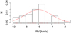 |
Fig. B.1. Gaussian fit of the RV distribution for ρ Oph after the 2σ clipping procedure. |
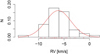 |
Fig. B.2. Gaussian fit of the RV distribution for the final selection of ρ Oph. |
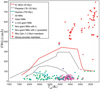 |
Fig. B.3. EW(Li)-versus-Teff figure for the final candidates of ρ Oph. All Li non-members are shown in open squares, of which we select giant and NG field contaminants of interest. |
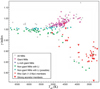 |
Fig. B.4. Gravity index γ as a function of Teff for ρ Oph. |
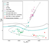 |
Fig. B.5. Kiel diagram for ρ Oph. We use the PARSEC isochrones with a metallicity of Z = 0.019. |
B.2. Chamaeleon I
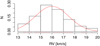 |
Fig. B.6. Gaussian fit of the RV distribution for Cha I after the 2σ clipping procedure. |
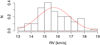 |
Fig. B.7. Gaussian fit of the RV distribution for the final selection of Cha I. |
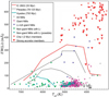 |
Fig. B.8. EW(Li)-versus-Teff figure for Cha I. |
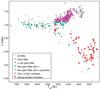 |
Fig. B.9. Gravity index γ as a function of Teff for Cha I. |
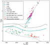 |
Fig. B.10. Kiel diagram for Cha I. |
B.3. γ Velorum
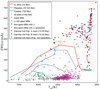 |
Fig. B.11. EW(Li)-versus-Teff figure for γ Velorum. |
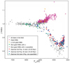 |
Fig. B.12. Gravity index γ as a function of Teff for γ Velorum. |
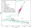 |
Fig. B.13. Kiel diagram for γ Velorum. |
B.4. NGC 2547
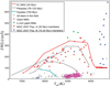 |
Fig. B.14. EW(Li)-versus-Teff figure for NGC 2547. |
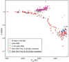 |
Fig. B.15. Gravity index γ as a function of Teff for NGC 2547. |
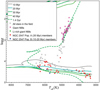 |
Fig. B.16. Kiel diagram for NGC 2547. |
B.5. IC 2391
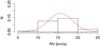 |
Fig. B.17. Gaussian fit of the RV distribution for IC 2391 after the 2σ clipping procedure. |
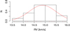 |
Fig. B.18. Gaussian fit of the RV distribution for the final selection of IC 2391. |
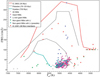 |
Fig. B.19. EW(Li)-versus-Teff figure for IC 2391. |
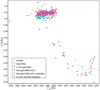 |
Fig. B.20. Gravity index γ as a function of Teff for IC 2391. |
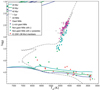 |
Fig. B.21. HR diagram for IC 2391. |
B.6. IC 2602
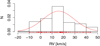 |
Fig. B.22. Gaussian fit of the RV distribution for IC 2602 after the 2σ clipping procedure. |
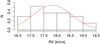 |
Fig. B.23. Gaussian fit of the RV distribution for the final selection of IC 2602. |
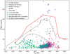 |
Fig. B.24. EW(Li)-versus-Teff figure for IC 2602. |
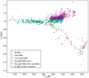 |
Fig. B.25. Gravity index γ as a function of Teff for IC 2602. |
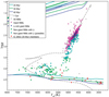 |
Fig. B.26. Kiel diagram for IC 2602. |
B.7. IC 4665
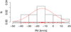 |
Fig. B.27. Gaussian fit of the RV distribution for IC 4665 after the 2σ clipping procedure. |
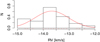 |
Fig. B.28. Gaussian fit of the RV distribution for the final selection of IC 4665. |
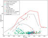 |
Fig. B.29. EW(Li)-versus-Teff figure for IC 4665. |
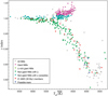 |
Fig. B.30. Gravity index γ as a function of Teff for IC 4665. |
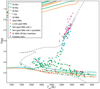 |
Fig. B.31. Kiel diagram for IC 4665. |
B.8. NGC 2516
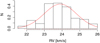 |
Fig. B.32. Gaussian fit of the RV distribution for NGC 2516. |
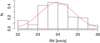 |
Fig. B.33. Gaussian fit of the RV distribution for the final selection of NGC 2516. |
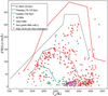 |
Fig. B.34. EW(Li)-versus-Teff figure for NGC 2516. |
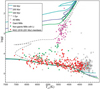 |
Fig. B.35. Kiel diagram for NGC 2516. |
B.9. NGC 6705
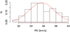 |
Fig. B.36. Gaussian fit of the RV distribution for NGC 6705. |
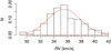 |
Fig. B.37. Gaussian fit of the RV distribution for the final selection of NGC 6705. |
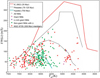 |
Fig. B.38. EW(Li)-versus-Teff figure for NGC 6705. |
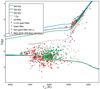 |
Fig. B.39. Kiel diagram for NGC 6705. |
B.10. NGC 4815
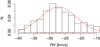 |
Fig. B.40. Gaussian fit of the RV distribution for NGC 4815. |
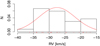 |
Fig. B.41. Gaussian fit of the RV distribution for the final selection of NGC 4815. |
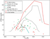 |
Fig. B.42. EW(Li)-versus-Teff figure for NGC 4815. |
 |
Fig. B.43. Kiel diagram for NGC 4815. |
B.11. NGC 6633
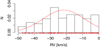 |
Fig. B.44. Gaussian fit of the RV distribution for NGC 6633. |
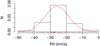 |
Fig. B.45. Gaussian fit of the RV distribution for the final selection of NGC 6633. |
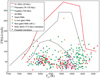 |
Fig. B.46. EW(Li)-versus-Teff figure for NGC 6633. |
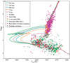 |
Fig. B.47. Kiel diagram for NGC 6633. |
B.12. Trumpler 23
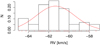 |
Fig. B.48. Gaussian fit of the RV distribution for Trumpler 23. |
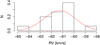 |
Fig. B.49. Gaussian fit of the RV distribution for the final selection of Trumpler 23. |
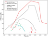 |
Fig. B.50. EW(Li)-versus-Teff figure for Trumpler 23. |
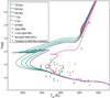 |
Fig. B.51. Kiel diagram for Trumpler 23. |
B.13. Berkeley 81
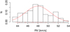 |
Fig. B.52. Gaussian fit of the RV distribution for Berkeley 81. |
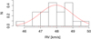 |
Fig. B.53. Gaussian fit of the RV distribution for the final selection of Berkeley 81. |
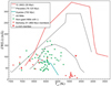 |
Fig. B.54. EW(Li)-versus-Teff figure for Berkeley 81. |
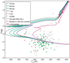 |
Fig. B.55. Kiel diagram for Berkeley 81. |
B.14. NGC 6005
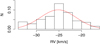 |
Fig. B.56. Gaussian fit of the RV distribution for NGC 6005. |
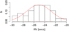 |
Fig. B.57. Gaussian fit of the RV distribution for the final selection of NGC 6005. |
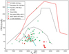 |
Fig. B.58. EW(Li)-versus-Teff figure for NGC 6005. |
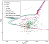 |
Fig. B.59. Kiel diagram for NGC 6005. |
B.15. NGC 6802
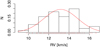 |
Fig. B.60. Gaussian fit of the RV distribution for NGC 6802. |
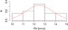 |
Fig. B.61. Gaussian fit of the RV distribution for the final selection of NGC 6802. |
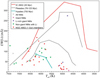 |
Fig. B.62. EW(Li)-versus-Teff figure for NGC 6802. |
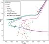 |
Fig. B.63. Kiel diagram for NGC 6802. |
B.16. Pismis 18
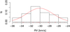 |
Fig. B.64. Gaussian fit of the RV distribution for Pismis 18. |
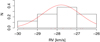 |
Fig. B.65. Gaussian fit of the RV distribution for the final selection of Pismis 18. |
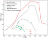 |
Fig. B.66. EW(Li)-versus-Teff figure for Pismis 18. |
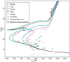 |
Fig. B.67. Kiel diagram for Pismis 18. |
B.17. Trumpler 20
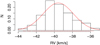 |
Fig. B.68. Gaussian fit of the RV distribution for Trumpler 20. |
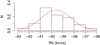 |
Fig. B.69. Gaussian fit of the RV distribution for the final selection of Trumpler 20. |
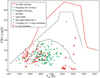 |
Fig. B.70. EW(Li)-versus-Teff figure for Trumpler 20. |
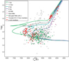 |
Fig. B.71. Kiel diagram for Trumpler 20. |
B.18. Berkeley 44
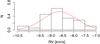 |
Fig. B.72. Gaussian fit of the RV distribution for Berkeley 44. |
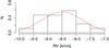 |
Fig. B.73. Gaussian fit of the RV distribution for the final selection of Berkeley 44. |
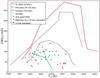 |
Fig. B.74. EW(Li)-versus-Teff figure for Berkeley 44. |
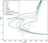 |
Fig. B.75. Kiel diagram for Berkeley 44. |
B.19. M67
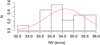 |
Fig. B.76. Gaussian fit of the RV distribution for M67. |
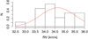 |
Fig. B.77. Gaussian fit of the RV distribution for the final selection of M67. |
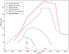 |
Fig. B.78. EW(Li)-versus-Teff figure for M67. |
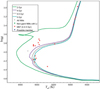 |
Fig. B.79. Kiel diagram for M67. |
B.20. NGC 2243
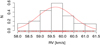 |
Fig. B.80. Gaussian fit of the RV distribution for NGC 2243. |
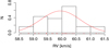 |
Fig. B.81. Gaussian fit of the RV distribution for the final selection of NGC 2243. |
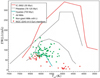 |
Fig. B.82. EW(Li)-versus-Teff figure for NGC 2243. |
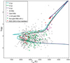 |
Fig. B.83. Kiel diagram for NGC 2243. Due to the metal-poor metallicity of this cluster we have considered PARSEC isochrones with Z = 0.006 instead of the usual near-solar metallicity of Z = 0.019. |
Appendix C: Tables with the full lists of cluster stars with membership analysis
Tables C.1–C.20 are available at the CDS.
All Tables
Age estimates, mean metallicity, distance to the Sun, and GES membership studies from the literature for the 20 clusters in our sample.
All Figures
|
Fig. 1. Distribution of radial velocities and RV selection for stars in the field of the cluster NGC 6705. Top panel: initial RV distribution for all the GES sources. We discard a few contaminants at the tails using the RStudioboxplot command (middle panel), and we show the Gaussian fit of the peak of the distribution using the 2σ clipping procedure around the median (bottom panel). |
| In the text | |
|
Fig. 2. Gaussian fit of the RV distribution of the members of the cluster NGC 6705 resulting from our membership analysis. |
| In the text | |
|
Fig. 3. EW(Li)-versus-Teff diagram showing the final candidate selection (red squares) for IC 2602, a 35-Myr-old cluster. The upper envelope of EW(Li) for the cluster IC 2602 is shown in red; the upper and lower envelopes of the Pleiades cluster are shown in grey; and the turquoise line represents the upper envelope of the Hyades cluster. For completeness we show here all field contaminants of interest, colour-coded as follows: RV non-members (open grey squares), Li-rich giants (blue), giant outliers which are not Li-rich, and finally (fuchsia), NG non-members (green) and possible candidates (turquoise). For more details, we refer the readers to Sects. 3.3 and 4). |
| In the text | |
|
Fig. 4. Kiel diagram of the GES sources (open squares) in the field of the cluster NGC 6705 (300 Myr). We indicate the candidate members with red squares, while the other coloured squares denote additional field contaminants of interest: Li-rich giants (blue), (non-Li-rich) giant outliers (fuchsia), and NG non-members with Li (green). We overplot the PARSEC isochrones for a metallicity of Z = 0.019 at 200 Myr (turquoise curve), 300 Myr (blue curve), 400 Myr (green curve), and 1 Gyr (gray dashed curve). |
| In the text | |
|
Fig. 5. Gravity-sensitive spectral index γ as a function of Teff for the sources (open squares) in the field of the SFR Cha I. The candidate members of Cha I are marked in red squares, while the other coloured squares denote the field contaminants of interest: Li-rich giants (blue), (non-Li-rich) giant outliers (fuchsia), NG non-members with Li (green), and potential NG outliers (turquoise – i.e., those in the 1.01 > γ > 1.0 range, see Sect. 4). As indicated by the dashed lines, we classified any stars with Teff < 5200 K and γ > 1.01. as giants. |
| In the text | |
|
Fig. 6. Histogram of [Fe/H] values for all the GES stars (red) in the field of the cluster NGC 6705, as well as the candidate members (blue) resulting from our analysis. The histogram shows an increasing dispersion towards the tails, confirming that this initial distribution is dominated by field stars. |
| In the text | |
|
Fig. 7. Distributions of [Fe/H] and Gaussian fits for the intermediate-age cluster NGC 6705. We display the histogram both for sources resulting from the 2σ clipping procedure on all the GES sources in this field (top panel), and for likely cluster members after applying all of our membership criteria (bottom panel). |
| In the text | |
|
Fig. 8. Panels from top to bottom: EW(Li), log g, and γ as a function of Teff for the Li-rich giant (blue squares), (non-Li-rich) giant (fuchsia squares), and NG (green squares) outliers in the field of the young clusters, in all cases without taking into account the rest of field stars. Turquoise squares indicate potential NGs in the 1.01 > γ > 1.0 range. |
| In the text | |
|
Fig. 9. EW(Li)-versus-Teff and Kiel diagrams for the Li-rich giant (blue squares), (non-Li-rich) giant (fuchsia squares), and NG (green squares) outliers in the field of the intermediate-age and old clusters in the sample. |
| In the text | |
|
Fig. 10. EW(Li)-versus-Teff diagrams for the candidate members of the young clusters (1–50 Myr; top panel), as well as the intermediate-age (50–700 Myr; middle panel) and old clusters (> 700 Myr; bottom panel). Open squares indicate possible members only, while inverted triangles refer to Li-rich members. |
| In the text | |
|
Fig. 11. Gravity index γ as a function of Teff for the young members in the young clusters of our sample. |
| In the text | |
|
Fig. 12. Kiel diagrams for the candidate members of the young clusters (1–50 Myr; top panel), as well as the intermediate-age (50–700 Myr; middle panel) and old clusters (> 700 Myr; bottom panel). We overplot the PARSEC isochrones in a similar age range, with a metallicity of Z = 0.019. Open squares indicate possible members only, while inverted triangles refer to Li-rich members. |
| In the text | |
|
Fig. B.1. Gaussian fit of the RV distribution for ρ Oph after the 2σ clipping procedure. |
| In the text | |
|
Fig. B.2. Gaussian fit of the RV distribution for the final selection of ρ Oph. |
| In the text | |
|
Fig. B.3. EW(Li)-versus-Teff figure for the final candidates of ρ Oph. All Li non-members are shown in open squares, of which we select giant and NG field contaminants of interest. |
| In the text | |
|
Fig. B.4. Gravity index γ as a function of Teff for ρ Oph. |
| In the text | |
|
Fig. B.5. Kiel diagram for ρ Oph. We use the PARSEC isochrones with a metallicity of Z = 0.019. |
| In the text | |
|
Fig. B.6. Gaussian fit of the RV distribution for Cha I after the 2σ clipping procedure. |
| In the text | |
|
Fig. B.7. Gaussian fit of the RV distribution for the final selection of Cha I. |
| In the text | |
|
Fig. B.8. EW(Li)-versus-Teff figure for Cha I. |
| In the text | |
|
Fig. B.9. Gravity index γ as a function of Teff for Cha I. |
| In the text | |
|
Fig. B.10. Kiel diagram for Cha I. |
| In the text | |
|
Fig. B.11. EW(Li)-versus-Teff figure for γ Velorum. |
| In the text | |
|
Fig. B.12. Gravity index γ as a function of Teff for γ Velorum. |
| In the text | |
|
Fig. B.13. Kiel diagram for γ Velorum. |
| In the text | |
|
Fig. B.14. EW(Li)-versus-Teff figure for NGC 2547. |
| In the text | |
|
Fig. B.15. Gravity index γ as a function of Teff for NGC 2547. |
| In the text | |
|
Fig. B.16. Kiel diagram for NGC 2547. |
| In the text | |
|
Fig. B.17. Gaussian fit of the RV distribution for IC 2391 after the 2σ clipping procedure. |
| In the text | |
|
Fig. B.18. Gaussian fit of the RV distribution for the final selection of IC 2391. |
| In the text | |
|
Fig. B.19. EW(Li)-versus-Teff figure for IC 2391. |
| In the text | |
|
Fig. B.20. Gravity index γ as a function of Teff for IC 2391. |
| In the text | |
|
Fig. B.21. HR diagram for IC 2391. |
| In the text | |
|
Fig. B.22. Gaussian fit of the RV distribution for IC 2602 after the 2σ clipping procedure. |
| In the text | |
|
Fig. B.23. Gaussian fit of the RV distribution for the final selection of IC 2602. |
| In the text | |
|
Fig. B.24. EW(Li)-versus-Teff figure for IC 2602. |
| In the text | |
|
Fig. B.25. Gravity index γ as a function of Teff for IC 2602. |
| In the text | |
|
Fig. B.26. Kiel diagram for IC 2602. |
| In the text | |
|
Fig. B.27. Gaussian fit of the RV distribution for IC 4665 after the 2σ clipping procedure. |
| In the text | |
|
Fig. B.28. Gaussian fit of the RV distribution for the final selection of IC 4665. |
| In the text | |
|
Fig. B.29. EW(Li)-versus-Teff figure for IC 4665. |
| In the text | |
|
Fig. B.30. Gravity index γ as a function of Teff for IC 4665. |
| In the text | |
|
Fig. B.31. Kiel diagram for IC 4665. |
| In the text | |
|
Fig. B.32. Gaussian fit of the RV distribution for NGC 2516. |
| In the text | |
|
Fig. B.33. Gaussian fit of the RV distribution for the final selection of NGC 2516. |
| In the text | |
|
Fig. B.34. EW(Li)-versus-Teff figure for NGC 2516. |
| In the text | |
|
Fig. B.35. Kiel diagram for NGC 2516. |
| In the text | |
|
Fig. B.36. Gaussian fit of the RV distribution for NGC 6705. |
| In the text | |
|
Fig. B.37. Gaussian fit of the RV distribution for the final selection of NGC 6705. |
| In the text | |
|
Fig. B.38. EW(Li)-versus-Teff figure for NGC 6705. |
| In the text | |
|
Fig. B.39. Kiel diagram for NGC 6705. |
| In the text | |
|
Fig. B.40. Gaussian fit of the RV distribution for NGC 4815. |
| In the text | |
|
Fig. B.41. Gaussian fit of the RV distribution for the final selection of NGC 4815. |
| In the text | |
|
Fig. B.42. EW(Li)-versus-Teff figure for NGC 4815. |
| In the text | |
|
Fig. B.43. Kiel diagram for NGC 4815. |
| In the text | |
|
Fig. B.44. Gaussian fit of the RV distribution for NGC 6633. |
| In the text | |
|
Fig. B.45. Gaussian fit of the RV distribution for the final selection of NGC 6633. |
| In the text | |
|
Fig. B.46. EW(Li)-versus-Teff figure for NGC 6633. |
| In the text | |
|
Fig. B.47. Kiel diagram for NGC 6633. |
| In the text | |
|
Fig. B.48. Gaussian fit of the RV distribution for Trumpler 23. |
| In the text | |
|
Fig. B.49. Gaussian fit of the RV distribution for the final selection of Trumpler 23. |
| In the text | |
|
Fig. B.50. EW(Li)-versus-Teff figure for Trumpler 23. |
| In the text | |
|
Fig. B.51. Kiel diagram for Trumpler 23. |
| In the text | |
|
Fig. B.52. Gaussian fit of the RV distribution for Berkeley 81. |
| In the text | |
|
Fig. B.53. Gaussian fit of the RV distribution for the final selection of Berkeley 81. |
| In the text | |
|
Fig. B.54. EW(Li)-versus-Teff figure for Berkeley 81. |
| In the text | |
|
Fig. B.55. Kiel diagram for Berkeley 81. |
| In the text | |
|
Fig. B.56. Gaussian fit of the RV distribution for NGC 6005. |
| In the text | |
|
Fig. B.57. Gaussian fit of the RV distribution for the final selection of NGC 6005. |
| In the text | |
|
Fig. B.58. EW(Li)-versus-Teff figure for NGC 6005. |
| In the text | |
|
Fig. B.59. Kiel diagram for NGC 6005. |
| In the text | |
|
Fig. B.60. Gaussian fit of the RV distribution for NGC 6802. |
| In the text | |
|
Fig. B.61. Gaussian fit of the RV distribution for the final selection of NGC 6802. |
| In the text | |
|
Fig. B.62. EW(Li)-versus-Teff figure for NGC 6802. |
| In the text | |
|
Fig. B.63. Kiel diagram for NGC 6802. |
| In the text | |
|
Fig. B.64. Gaussian fit of the RV distribution for Pismis 18. |
| In the text | |
|
Fig. B.65. Gaussian fit of the RV distribution for the final selection of Pismis 18. |
| In the text | |
|
Fig. B.66. EW(Li)-versus-Teff figure for Pismis 18. |
| In the text | |
|
Fig. B.67. Kiel diagram for Pismis 18. |
| In the text | |
|
Fig. B.68. Gaussian fit of the RV distribution for Trumpler 20. |
| In the text | |
|
Fig. B.69. Gaussian fit of the RV distribution for the final selection of Trumpler 20. |
| In the text | |
|
Fig. B.70. EW(Li)-versus-Teff figure for Trumpler 20. |
| In the text | |
|
Fig. B.71. Kiel diagram for Trumpler 20. |
| In the text | |
|
Fig. B.72. Gaussian fit of the RV distribution for Berkeley 44. |
| In the text | |
|
Fig. B.73. Gaussian fit of the RV distribution for the final selection of Berkeley 44. |
| In the text | |
|
Fig. B.74. EW(Li)-versus-Teff figure for Berkeley 44. |
| In the text | |
|
Fig. B.75. Kiel diagram for Berkeley 44. |
| In the text | |
|
Fig. B.76. Gaussian fit of the RV distribution for M67. |
| In the text | |
|
Fig. B.77. Gaussian fit of the RV distribution for the final selection of M67. |
| In the text | |
|
Fig. B.78. EW(Li)-versus-Teff figure for M67. |
| In the text | |
|
Fig. B.79. Kiel diagram for M67. |
| In the text | |
|
Fig. B.80. Gaussian fit of the RV distribution for NGC 2243. |
| In the text | |
|
Fig. B.81. Gaussian fit of the RV distribution for the final selection of NGC 2243. |
| In the text | |
|
Fig. B.82. EW(Li)-versus-Teff figure for NGC 2243. |
| In the text | |
|
Fig. B.83. Kiel diagram for NGC 2243. Due to the metal-poor metallicity of this cluster we have considered PARSEC isochrones with Z = 0.006 instead of the usual near-solar metallicity of Z = 0.019. |
| In the text | |
Current usage metrics show cumulative count of Article Views (full-text article views including HTML views, PDF and ePub downloads, according to the available data) and Abstracts Views on Vision4Press platform.
Data correspond to usage on the plateform after 2015. The current usage metrics is available 48-96 hours after online publication and is updated daily on week days.
Initial download of the metrics may take a while.