| Issue |
A&A
Volume 643, November 2020
|
|
|---|---|---|
| Article Number | A40 | |
| Number of page(s) | 22 | |
| Section | Planets and planetary systems | |
| DOI | https://doi.org/10.1051/0004-6361/201936227 | |
| Published online | 29 October 2020 | |
A new equation of state applied to planetary impacts
II. Lunar-forming impact simulations with a primordial magma ocean
1
Lund Observatory, Department of Astronomy and Theoretical Physics, Lund University,
Box 43,
22100
Lund, Sweden
e-mail: This email address is being protected from spambots. You need JavaScript enabled to view it.
2
Institute of Theoretical Astrophysics, University of Oslo,
Postboks 1029,
0315
Oslo,
Norway
e-mail: This email address is being protected from spambots. You need JavaScript enabled to view it.
Received:
2
July
2019
Accepted:
11
August
2020
Abstract
Observed FeO/MgO ratios in the Moon and Earth are inconsistent with simulations done with a single homogeneous silicate layer. In this paper we use a newly developed equation of state to perform smoothed particle hydrodynamics simulations on the lunar-forming impact, testing the effect of a primordial magma ocean on Earth. This is investigated using the impact parameters of both the canonical case, in which a Mars-sized impactor hits a non-rotating Earth at an oblate angle, and the fast-rotating case, in which a half-sized Mars impactor hits a fast-spinning Earth head-on. We find that the inclusion of a magma ocean results in a less massive Moon and leads to slightly more mixing. Additionally, we test how an icy Theia would affect the results and find that this reduces the probability of a successful Moon formation. Simulations of the fast-spinning case are found to be unable to form a massive-enough Moon.
Key words: equation of state / planets and satellites: formation / planets and satellites: dynamical evolution and stability / planets and satellites: interiors / Moon / Earth
© ESO 2020
1 Introduction
During the late stages of planet formation, it is believed that the inner Solar System was populated by planetary embryos with masses ranging from 0.01 to 0.2 Earth masses (Mars-like; Ida & Makino 1993). For a planet to grow much larger than this, collisions between planetary embryos are believed to be necessary (Goldreich et al. 2004). Several of these giant collisions resulted in the Earth, and the last one is believed to have been the lunar-forming impact (Hartmann & Davis 1975; Cameron & Ward 1976). In addition to fitting neatly into planetary formation models, this scenario also explains many of the observed physical traits of the Earth–Moon system (i.e., correct Moon mass and angular momentum of the current Earth–Moon system, and the small iron core of the Moon; Canup & Asphaug 2001). There are several variants and models of the giant impact theory, the most famous one being the “canonical” one (Benz et al. 1989; Canup 2004), in which a planet called Theia hit the Earth at around a 45-degree impact angle resulting in a disc of material that eventually coalesced into the Moon (Canup & Asphaug 2001). This model correctly captures many of the dynamical aspects of the Earth–Moon system, but fails to reproduce the isotopic similarity of the Earth and Moon found from observations (Wiechert et al. 2001; Zhang et al. 2012); in the canonical model, most of the mass that created the Moon came from Theia, which would most likely have had a different isotopic ratio, and certain isotope ratios are very sensitive to their initial birth environment in the protoplanetary disk (Pahlevan & Stevenson 2007). This has led to other variants of the giant-impact theory, the most prominent ones being: the merger theory (Canup 2012), which predicts that the Moon formed from the debris left by a merger between two half-sized Earths; the fast-spinning theory (Ćuk & Stewart 2012), in which a smaller Theia collides with a fast-spinning proto-Earth that flung material out to create the Moon; and the hit-and-run model (Reufer et al. 2012), in which a substantial amount of Theia escapes orbit, leaving a disc that is less enriched with Theia than in the canonical model. The first two variations are referred to as high-angular-momentum theories as the resulting system has an angular momentum that is far above the one we have today. Fast-spinning theory argues that this is due to subsequent momentum loss caused by evection resonance (Touma & Wisdom 1998; Ćuk & Stewart 2012). These two models produce the correct isotopic ratios, but are problematic when it comes to reproducing the chemical differences between Earth and the Moon. In comparison to Earth, the Lunar mantle is depleted in volatile and siderophile elements (Jones & Palme 2000), which includes a difference in the content of FeO (Earth: 7.67% vs. Moon: 10.6%; Warren & Dauphas 2014). Because of the highly mixed end-state of the high-angular-momentum models, this FeO difference cannot have originated from the lunar-forming impact itself and requires either a post-impact self-oxidation of the lunar mantle (Wade & Wood 2005), oxidation by a late veneer, or chemical fractionation in the post-impact disc (Pahlevan et al. 2011). It is unlikely that self-oxidation of the lunar mantle or oxidation by a late veneer would be more important on the Moon than on the Earth (Meier et al. 2014). Pahlevan et al. (2011) showed that chemical fractionation can occur in the post-impact disc due to rainout in convective clouds; however, this requires that the turbulent mixing occur faster than the transfer of angular momentum within the disk (Melosh 2009), and whether or not this happens is still uncertain. Further post-disc simulations are required to gauge the effect of chemical fractionation. In the case of the canonical model, the chemical difference can be more easily explained because the difference produced depends heavily on the composition of Theia. To obtain the correct isotope ratios in this latter case would require that proto-Earth and Theia have almost identical isotope ratios to begin with; this has been argued to be the case by some authors (Mastrobuono-Battisti et al. 2015; Dauphas 2017), but is considered unlikely by others (Pahlevan & Stevenson 2007; Kaib & Cowan 2015). Another possible solution was presented by Karato (2014), which suggested that the primordial magma ocean on Earth would have been enriched in FeO as melting changes the chemical composition. If large amounts of magma were flung into orbit, this could explain the richness in FeO that we see in the Moon today. All of the simulations mentioned above only used two homogeneous layers (iron core and silicate mantle) to describe the collision, neglecting the modeling of a magma ocean. Asymmetric shock heating would have been important if the Earth had amolten surface while Theia did not. The liquid has a higher Gruneisen parameter and is more easily compressed than its solid counterpart, leading to asymmetric heating at impact and a higher pressure gradient from the molten surface. From planetary studies, a Mars-like planet like Theia would not have had a molten surface (Sasaki & Nakazawa 1986). While the Earth is predicted to have had a molten surface of at least 300 km in depth (Abe 1997).Our numerical simulations test the effect of a proto-Earth with a molten surface compared to that of a solid surface. Thesimulations also test a wide array of different impact conditions. This includes simulations done in accordance with the setup of both the canonical case (Canup 2004) and from the fast-spinning case (Ćuk & Stewart 2012). In addition, we look at the difference between two models of Theia, a rocky and an icy one. An icy Theia would have had to migrate inward from the outer Solar System, just like Ceres is believed to have done (McKinnon 2008; Walsh et al. 2011). Concurrent to the development of the work presented in this paper, Hosono et al. (2019) presented results from numerical simulations of lunar-forming impacts with a terrestrial magma ocean. We discuss the results of the two models and differences between them in Sect. 5.
In Sect. 2 we explain the setup of the simulations. In Sect. 3 we discuss the post-analysis of the simulations and perform a compositional analysis of the lunar-forming impact. In Sect. 4 the results of our simulations are presented and in Sect. 5 we discuss the different results. We finally end with some conclusions.
2 Simulation setup
Simulations of the lunar-forming impact were done using smoothed particle hydrodynamics (SPH; Lucy 1977; Gingold & Monaghan 1977), with the astrophysical code VINE (Wetzstein et al. 2009). The equation of state (EOS) was implemented within VINE and the default internal energy evolution was replaced with a temperature evolution. Material strength can be ignored, as the kinetic energy of the lunar-forming impact exceeds the yield strength of the materials (Asphaug et al. 2015). We use a C4 Wendland kernel that has been shown to be resistant against the pairing instability (Dehnen & Aly 2012). This allows for a higher neighbor count (around 200), which improves the convergence of SPH. To model shock dissipation in SPH the artificial viscosity (AV) switch prescription of Morris & Monaghan (1997) is used.
2.1 Planetary models
The density profiles of the different models of proto-Earth and Theia were attained from the same method presented in paper 1. We used eight proto-Earth models in our simulations. This includes either a multi-layered (4 main layers) or a simple-layered (2 main layers) proto-Earth with either a molten (PEM) or solid (PES) surface with a mass of either MP = 0.95ME or MP = 1.05ME.
The multi-layered PES model consists of four layers, inner core (IC), outer core (OC), lower mantle (LM), and upper mantle (UM). The IC, OC, and LM are taken to be the same as the fitted values from the preliminary reference Earth model (PREM; see paper 1). The UM is taken to be made of olivine, which is the most abundant mineral in Earth’s upper mantle. The central pressure and temperature are taken to be the same as in the PREM model (see paper 1) in order to keep the conditions of the inner regions of the planet roughly the same for all the models. The simple-layered PES model is constructed with only the IC material and the UM material (olivine). To achieve a surface temperature of around 1000 K in both PES models, we add a small temperature discontinuity at the core–mantle boundary.
The multi-layered PEM model consists of exactly the same material layers with the addition of a surface magma layer that has a depth of around 300–500 km (Abe 1997). The magma layer is modeled after the olivine melt. We get the olivine material and melt data from several sources (Stixrude & Lithgow-Bertelloni 2005; Jing & Karato 2011; Thomas et al. 2012; Costa et al. 2017). We use the same central pressure and temperature as the PES model, however we do not include any temperature discontinuity at the core–mantle boundary. The simple-layered PEM model is constructed with only the IC material, the UM material (olivine), and the magma layer. In both models, the surface temperature ends up being around 2000 K.
We also have a test model which is the same as the two-layered model, except with its material vaporization energy set to triple the original value. This is done to gauge the effect of the expanded state model in the EOS.
In the case of Theia, we have three models. Two of these are different in that they have different sizes and mass (M = 0.142ME, M = 0.05ME), which are the same masses as the ones used by Canup (2004) and Ćuk & Stewart (2012). These two models consider only two layers, an iron core (modeled as the inner core PREM model) representing a third of the planet’s mass, and an olivine mantle representingthe rest. The core pressure and temperature are adjusted to give the desired mass and surface temperature (T ≈ 1000 K) of the planet. We call these the rocky Theia models. The theother Theia model represents an “icy” Theia with density and properties modeled based on CI-chondrite meteorites and planetary data from Ceres (Thomas et al. 2005; Park et al. 2016). We make a rather simple model of the “icy” material. CI-chondrites are made out of several different silicates and water-bearing phyllosilicates, with the most abundant silicate being olivine. We decided to determine the material properties of our icy material from a weighted average between olivine and ice from material parameters taken from Stixrude & Lithgow-Bertelloni (2005) and Weppner et al. (2015). We fit the values to a core that has around ρ = 2600 ↔ 2300 kg m−3 and a mantle that has around ρ = 1600 ↔ 2000 kg m−3, leaving us with a total bulk density of ρ = 2200 kg m−3, just as was measured for Ceres. All the planets and their material layers together with respective ambient pressure values are given in Appendix A.
2.2 Distribution of particles
Shells are distributed radially outward by the method described in Appendix B. Given the density profile and a chosen number of particles N, we can determine the number of shells and the number of particles per shell. All our particles have the same mass, as unequal masses produce numerical artifacts in very mixed cases (Rasio & Lombardi 1999). The particles are distributed in a spiral pattern on the shells following the prescribed method of Saff & Kuijlaars (1997).
Ideally one would like an initial distribution that is isotropic and that follows the true density profile. From Fig. 1 we can see that the distribution follows the density profile quite well. However, the distribution is not completely isotropic: there is a bias near the discontinuities. On the high-density side, the distance to the closest neighbors on the shell is smaller than the distance to the closest neighbors between shells. The opposite is true on the low-density side. However, without changing the particle masses or implementing first-order corrections to the kernel (Reinhardt & Stadel 2017) this small bias in the initial distribution is more desirable than a poor density fit. Letting the distribution relax and equilibrate will minimize the bias. The distribution is relaxed until the mean speed of the particles is below a fraction of the impact speed ( ). From Fig. 1 we can see that doing the relaxation of our planet gives a good fit to the planet’s true density profile despite having several density discontinuities to deal with.
To investigate the effect of rotation in impacts, we also add spin to our proto-Earth models. For the sake of comparison, we choose the rotations based on the ones used by Ćuk & Stewart (2012). We spin up the planets by incrementally adding angular momentum to the planet and letting it relax. This is done to reduce any unwanted particle disorder and to reduce the error in the total energy. We begin by spinning it up to a period of 6h, then further to 3, 2.5, and finally to 2.3 h1. When relaxing the rotating planet we instead stop the relaxation when the z-component of the velocity goes to a fraction of the impact speed. The flattening and equatorial radius of the spun up proto-Earth are  and Req = 8500 km respectively, which is in line with the initial conditions from Ćuk & Stewart (2012).
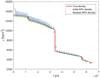 |
Fig. 1 Depiction of the initial condition of the M = 1.05ME multi-layered PES model. Here, we show how the true density compares with the approximated density from the SPH summation formula. The initial SPH density is given from the initial distribution of particles using the method described in Appendix B. The density after relaxation is given by the green curve. We can see that in general we get a very good fit; however, we do get a slight a gap between the density discontinuities, which is characteristic of the artificial surface tension effect (Agertz et al. 2007). |
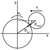 |
Fig. 2 Top-down view of an impact, highlighting the important parameters involved in the collision. |
2.3 Impact parameters
The collision is set up as seen in Fig. 2. The target planet is denoted with subscript “tar” and the impactor is denoted with subscript “imp”. Other than the mass (Mtar, Mimp), radius (Rtar, Rimp), and material properties of the two bodies (Appendix A), there are three important parameters to consider. The first is the velocity at impact vimp:
 (1)
(1)
where vesc is the escape velocity, which is the velocity that a body would attain from just the gravitational attraction of the other, if they started out at rest and infinitely far apart from each other, and vinf is the velocity at infinity which is any excess velocity that the body might have gained apart from the escape velocity. The second important parameter is the angle between the two planetary surfaces at the point of impact ξ, which is often written as an impact parameter b:
 (2)
(2)
The third involves the spin of the target planet ωz (or impactor) around the equatorial plane z. The spin can either be prograde or retrograde. We set up our spin on the planets such that b > 0 represents prograde impacts and b < 0 represents retrograde impacts. All of our impacts are aligned to the equatorial plane of the target planet z = 0.
We either choose vimp and b directly, or we infer vimp by choosing b and a desired angular momentum for the impact:
 (3)
(3)
where Limp is the total angular momentum involved in the impact, Lcol represents the initial orbital angular momentum, and Lω represent the spin angular momentum of the planets. By setting a desired Limp we can then get vimp from Lcol (Canup 2008a).
3 Impactanalysis
The success of an impact is evaluated based on constraints given by the current Earth–Moon system.
- 1.
The resulting planet (MP) and satellite (Mm) must have a mass similar to that of Earth (ME = 5.98 × 1024 kg) and the Moon (MM = 7.35 × 10²² kg).
- 2.
The final angular momentum must be greater than or equal to the current Earth–Moon system (LEM = 3.5 × 1034 kg m2 s−1)2.
- 3.
The resulting satellite must replicate the iron deficiency of the Moon (δFE < 10%).
- 4.
Given the isotopic composition of Theia, the impact must reproduce the similarity in isotopic ratios of the Earth and the Moon (δfT).
- 5.
The resulting planet and satellite must have plausible relative FeO/MgO ratios for proto-Earth (Qtar,solid) and Theia (Qimp).
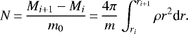
After the impact, a disk of material will form around the Earth. A fraction of the material in the disk will eventually coalesce and form the Moon. The subsequent viscous evolution of the disk is not simulated; instead we use the empirical results of Ida et al. (1997); Kokubo et al. (2000) to determine the mass of the Moon.
![Mathematical equation: \begin{equation*}M_m\,{=}\,\frac{1.9L_D}{\sqrt[]{2.9GM_E R_E}}-1.1M_D-1.9M_{D,\textrm{esc}} ,\end{equation*}](/articles/aa/full_html/2020/11/aa36227-19/aa36227-19-eq6.png) (4)
(4)
where MD and LD are the mass and angular momentum of the disk, respectively, and MD,esc is the estimated mass that is lost during its evolution. This latter is usually taken to be zero or 5% of the disk mass. Using an iterative process from Canup & Asphaug (2001), the SPH particles are classified as either planet, disk, or escapees. The particles are assumed to undergo energy dissipation due to mutual particle collision leading to circular orbits. Planet particles have a semi-major axis that is less than the equatorial radius of the planet3. Escapees have enough kinetic energy to become gravitationally unbound, and the remaining particles are disk particles. The angular momentum of the planet and disk particles then gives the total angular momentum of the bound system (Lsys). The fraction of iron particles in the disk determines the iron abundance of the resulting satellite (δFE). To clarify the subscript notation: the deviation in the isotopic composition of the resulting planet and satellite can be determined using a mass balance equation and the epsilon notation (Canup 2012):
 (5)
(5)
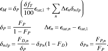
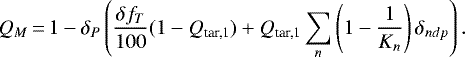
where FD and FP are the mass fractions of silicate material from the target planet in the resulting disk and planet, respectively, and δfT represents the percentage compositional deviation of the disk from the resulting planet, such that a δfT = 0 represents a disk with an equal fraction of target material as in the resulting planet. The required FeO/MgO ratios of proto-Earth and Theia can be determined using a similar method. A generalized expression can be developed for n materials with different compositions (Appendix C). In the case of the PEM model, we require two different proto-Earth materials, one solid and its respective melt. The FeO-to-MgO ratio for the Moon and the Earth becomes:
 (6)
(6)
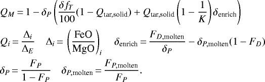
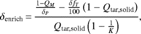
Here, subscript solid and molten represents the solid and molten silicate material, respectively, FP,molten and FD,molten are the mass fractions of molten material from the target planet in the resulting planet and disk, K is the exchange function with respect to the solid material (olivine), δenrich estimates the effective enrichment of FeO/MgO in the resulting disk, δP,molten describes how much of the resulting planet is composed of the molten part, and δP describes how much target material versus impactor material ends up in the resulting planet. We can calculate QM, ΔE, Δm from the FeO and MgO abundances on Earth and the Moon (Warren 2005):

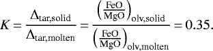
The exchange function of olivine and its melt has its average at 0.35 (Mibe et al. 2006):
 (7)
(7)
After a simulation we can calculate δP, δfT, and δenrich. Together with the value of QM we can calculate Qtar,solid from Eq. (6). Concurrently this also gives Qimp.
Before we continue to the simulation results, we investigate which collisions give satisfactory isotope and FeO/MgO ratios. The equations that are of interest in this analysis are as follows.
 (8)
(8)
![Mathematical equation: \begin{equation*}Q_{\textrm{imp}}\,{=}\,1+\delta_P\left[1-Q_{\textrm{tar,solid}}+\delta_{P,\textrm{molten}}Q_{\textrm{tar,solid}}\left(1-\frac{1}{K}\right)\right] .\end{equation*}](/articles/aa/full_html/2020/11/aa36227-19/aa36227-19-eq12.png) (9)
(9)
Because of the isotopic similarity between the Earth and the Moon, the parameter δfT is restricted depending on the isotopic composition of Theia. Meier et al. (2014) and Herwartz et al. (2014) give the required criterion parameter for δfT for CI-chondrite, Angrite, Vesta, Mars, and Enstatite composition:
In Canup (2012), an upper value of the isotopic composition of Theia is taken to be one-eighth of Mars which then gives a criterion of:
To further restrict our parameter space, we set a realistic maximum and minimum FeO/MgO ratio of our impactor. A realistic maximum FeO content would be around 30% (Meier et al. 2014), which would correspond to a FeO/MgO ratio of around unity. This then gives us Qimp,max ≈ 5 (about double that of Mars: QMars ≈ 2.6). The minimum is set to the limiting value of Q = 0. We choose three values of δP to look at. High, intermediate, and low values are chosen to represent the different cases: Low δP = 4, Intermediate δP = 8, High δP = 16. Finally we set a restriction on δP,molten. We also choose three values here: one which represents the removal of all molten material from the planet δP,molten = 0, an intermediate value of δP,molten = 0.15, and a high value of δP,molten = 0.3. Given QM and the partition function K together with all of the restrictions, we solve Eqs. (8) and (9) for a range of different Qtar,solid values. The result of the analysis is plotted in Fig. 3 (δP = 8 and the restis given in Appendix C). From this, we can see that the addition of a molten ocean opensup more possibilities in different compositions of Theia and proto-Earth. The parameters δenrich = 0 and δP,molten = 0 represents the classical Theia–Earth collision with only one target silicate material. We can see from Fig. 3 that the classical Theia–Earth collision is only possible for the enstatite composition case, requiring a Qtar,solid close to unity and a high Qimp. Increasing δP,molten leads to a larger range in the δenrich parameter, but restrictsQtar,solid to smaller ranges and values. Another trend that can be seen is the effect of increasing δP, which reduces the range of Qtar,solid but decreases the required value of δenrich for the smaller |δfT| values. Figure 4 shows the allowed composition of the impactor for different kinds of δP. As we can see, an increase in δP narrows the range of possible Qtar,solid values.
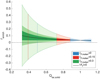 |
Fig. 3 Result of the compositional analysis with δP = 8. The blue, red, and green areas represent the cases in which the ratios of molten material in the resulting planet are δP,molten = 0, 0.15, 0.3 respectively.The vertical red and blue lines represent the extent of the red and blue areas. The light colors represent |δfT | < 40%, medium colors represent |δfT| < 13%, and dark colors represent |δfT| < 6%. The black dashed line highlights δenrich = 0 and the black solid line highlights |δfT| = 0. |
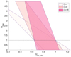 |
Fig. 4 Allowed values for the relative FeO/MgO of the target planet and impactor for different δP. The boundary line to the right of each shaded area represents δP,molten = 0 and the boundary line to the left represents δP,molten = 0.3. |
4 Simulation results
We divide the simulation results into two sections. The first outlines simulations done on a nonrotating proto-Earth, which we call the “canonical case” (denoted “c”). In the second section, called the “fast-spinning case” (denoted “f”) we outline simulations of a rapidly rotating proto-Earth with a period of 2.3 h ↔ 3 h. We make use of the models and methods that we have described in the previous sections and investigate the effect of different impact parameters and planetary compositions on the resulting Moon. All the rendered figures in the upcoming sections were visualized using SPLASH (Price 2007).
4.1 Canonical case
We performed 65 simulations of the lunar-forming impact with a nonrotating proto-Earth with a mass of Mtar = 0.95ME and an impactor with a mass of Mimp = 0.142ME. A total of 12 simulations were run with the simple-layered proto-Earth model (Tables A.6, A.7) together with the rocky Theia model (Table A.9) at a high resolution of N = 3.3 × 10⁶ particles (simulations referred to as Hdrc#Solid/Molten). A total of 53 simulations were run with the multi-layered proto-Earth model (Tables A.4, A.5) where 6 simulations were run with high resolution N = 3.3 × 10⁶ particles (simulations referred to as Hrc#Solid/Molten). One simulation was run with N = 1.2 × 10⁶ particles (Mrc1Solid) to check convergence. Also, 46 simulations were done with low resolution N = 1.2 × 10⁵ particles, 30 of which were run with the rocky Theia model (simulations referred to as Lrc#Solid/Molten) and the rest with the icy Theia model (Table A.10), these simulations are denoted as Lic#Solid/Molten. For each simulation, the impact angle and angular momentum of the impact was varied. Each of the simulations ran for 24 h and their results can be seen in Table 1.
In Figs. 5–10 we show the evolution of the high-resolution case: “Hrc1Solid”. In this case, the proto-Earth is modeled using the multi-layered PES model together with a rocky Theia. Figure 5 shows the pre-impact conditions from an equatorial view and a top-down view. The color rendering shows the temperature of each SPH particle. The impact parameter and angular momentum are in this case set to b = 0.3 and Li = 1.25LEM respectively. In Fig. 6 we see the state of the simulation in the top-down view at different times (t = 0.25, 1, 2, 5, 7.5, 15h). The impactor can be seen hitting in an oblique angle which results in shearing of the impactor. The impact leads to the formation of a pressure wave bulge that starts to go around the planet, a stream of infalling material follows right behind, heating the planet. At around t = 2 h, the wave bulge starts to collapse into the planet which releases a large amount of heat energy. At t = 5 h, the planet is rotating rapidly and the sheared-off material has developed into a stream that extends out from the planet. In the stream, we can see several satellites have started to form, especially the large satellite seen in the bottom left of t = 5 h which has approximately the mass of the Moon. The collapse of the initial wave bulge forms another pressure wave that goes around the planet. This pressure wave hits the tidal stream at t = 5 h which creates a strong torque on the infalling stream, and together with the high outward pressure from the heated vaporized surface, the stream is pushed into a larger orbit, which can be seen in t = 7.5 h. After t = 12 h, the large satellite is on a course to recollide with the planet. This eventually shears off some additional material into orbit which can be seen in Fig. 7, where the state of the system after t = 24 h is presented. The temperature profile of the inner r < 1Re is plotted in Fig. 10 before and after impact (for both the multi-layered case and the simple-layered case). The planet with its extended vaporized atmosphere has temperatures in the range of 3 × 10³ ↔ 3 × 10⁴ K with an average temperatureof Tavg = 5604 K.
Figure 8 shows a color rendering of the density at the end of the simulation from a top-down view and an equatorial view. We can see a disk-like structure around an almost spherical inner planet. Several small satellites can be seen in the extending material stream. Figure 9 shows the distribution of iron and silicate at the end of the simulation. This figure also shows the result from our disk analysis. Assuming no mass loss from the subsequent disk evolution, we get an estimated Moon mass of Mm = 1.19MM, and with a mass loss of around 5% in the disk evolution we get an estimated Moon mass of Mm = 1.02MM. The stream of particles that extends out from the planet mostly consists of impactor material. This is reasonable as the materialcomes mostly from the larger satellite, which was formed early on from the sheared-off impactor material that collided late in the simulation. The composition of the disk is dominated by impactor material with δfT = −52%; the iron content is below 10% and the estimated relative FeO/MgO ratio of the impactor and target is Qtar,solid = 0.88, Qimp = 1.95. The high δfT requires an impactor that has near-identical isotopic ratios to that of Earth. The iron content and the Q ratio are however well within the acceptable ranges. The angular momentum of the bounded system is slightly higher than the Earth–Moon system, namely Lsys = 1.23LEM.
Figure 11 shows the impact properties of all the simulations from Table 1. A description of each symbol, color, and size is given in the caption. In Fig. 11a we can see a linear relationship between the disk mass and its angular momentum. Fitting the Lrc# data to a polynomial we find LD = 0.1745MD. Rewriting Eq. (4) in terms of Lem and Mm and inserting the relationship into the equation we get Mm ≈ 0.74MD. Fitting to the Hdrc# data and we get LD = 0.1733MD and Mm ≈ 0.73MD and fitting to the Lic# data we get LD = 0.1575MD and Mm ≈ 0.56MD.
System properties of the canonical impact simulations.
4.2 Fast-spinning case
We performed 28 simulations of the Moon-forming impact with a fast-rotating proto-Earth with a mass of Mtar = 1.05ME and an impactor with a mass of Mimp = 0.05ME. All simulations used about N = 3.1 × 10⁵ SPH particles. The proto-Earth was in each case modeled using the multi-layered PES or PEM model described in Sect. 2.1 (Tables A.1 and A.2). These simulations are denoted Lrf#Solid/Molten. For six simulations, we used a simpler, two-layered model of a proto-Earth (Table A.3). These simulations are denoted Lrdf#Solid/Molten. Additionally, an extra two-layered model was made which was the same as the regular two-layered model but with material that had three times the vaporization energy. This simulation is denoted  . All the simulations used a rocky planetary model for Theia (Table A.8). For each simulation the impact angle, impact velocity, and rotation of the target planet were varied. The simulations ran for 24 h and their results can be seen in Table 2.
In Figs. 12–17 we show the evolution of the fast-spinning case of “Lrf12Molten”. In this case, the proto-Earth is modeled using the multi-layered PEM model. Figure 12 shows the pre-impact conditions from an equatorial view and a top-down view. From the very oblate target planet, we can see that the planet is spinning very rapidly. The color rendering shows the temperature of each SPH particle, and the color–temperature range can be seen in Fig. 12. The spin period, impact velocity, and angular momentum are set to P = 2.3 h, b = −0.3, and vimp = 20 km s−1 respectively.These starting values are taken from simulations done by Ćuk & Stewart (2012). Figure 13 shows the state of the simulation in the top-down view at different times (t = 0.25, 1, 2, 5, 7.5, 12 h). The impactor can be seen hitting the target head-on, which creates a strong shock-wave that propagates through the planet. Much of the impactor is swallowed by the target planet; however, there is also a significant amount that is scattered in the z-direction (which can better be seen from Fig. 17). As the planet falls in on itself due to its rapid rotation, it creates a torque and starts to fling material out into orbit. Similar to the canonical case we have a tidal bump that goes around the planet (albeit much smaller). After about 12 h the post-impact has calmed down, and we are left with a very hot planet and atmosphere. The average temperature of the planet and atmosphere is Tavg = 7700 K, which is a significant increase compared to the canonical model. In these kinds of simulations, we are not left with any distinct stream of particles; instead we have a more isotropic distribution around the planet (see Fig. 14).
Figure 16 shows the distribution of iron and silicate content of the target and impactor material. This figure also shows the result from our disk analysis. Assuming no mass loss from the disk, we get an estimated Moon mass of Mm = 0.13MM. We can also see that this type of simulation has a much more even distribution of the target and impactor material, leading to a lower δfT = −8%. The iron content in the disk is below 10% and the estimated FeO/MgO of the impactor and target is Qtar,solid = 0.3, Qimp = 6.09. The angular momentum of the bounded system is much higher than the Earth–Moon system Lsys = 2.68LEM. However, most of this comes from the planet and only LD = 0.06LEM is in the disk.
This type of collision has been seen to produce Moon-like satellites by Ćuk & Stewart (2012); Nakajima & Stevenson (2014), but none of our simulations show this (see Fig. 18). To figure out the reason for this discrepency, we performed several different tests. First we made a simpler model of the proto-Earth using only two layers, which is similar to the one used by Ćuk & Stewart (2012). We find however that this does not significantly change the result (ΔMm ≈ 0.02MM between the Lrf12Solid and Lrdf1Solid case). We see a small increase in the mass of the disk (ΔMD ≈ 0.07MM) and less mass escapes (ΔMesc ≈−0.43MM), but about the same angular momentum resides in the disk (LD = 0.09LEM). This model does not therefore fix the discrepancy between the results. Next, we increased the vaporization energy of our silicate material to see if this had any effect. This also does not change the result significantly (ΔMm ≈ 0.03MM between the Lrdf1Solid and  case). We see a further increase in the disk mass (ΔMD ≈ 0.08MM) and even less mass escapes the system (ΔMesc ≈−0.43MM). We also see a small increase in the disk angular momentum (ΔLD = 0.02LEM).
Figure 18 shows the impact properties of all the simulations in Table 2. A description of each symbol, color, and size is given in the caption. In Fig. 18a we can see a linear relationship between the disk mass and its angular momentum. Fitting the data to a polynomial we find LD = 0.1327MD. By inserting this value into Eq. (4), we obtain Mm ≈ 0.3MD.
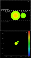 |
Fig. 5 Initial setup of the Hrc1Solid simulation. The impact parameter and angular momentum are in this case set to b = 0.3 and Limp = 1.25LEM respectively.The color rendering represents the temperature. Upper figure: equatorial view of the initial setup. The cross section that can be seen represents the region in which particles are rendered, which is done to improve the clarity of the following figures. Lower panel: top-down view of the initial setup and is the viewpoint in the following figures. |
5 Discussion
From the compositional analysis in Sect. 3 we saw that the classical Earth–Theia collision could only be satisfied for higher fractions of impactor material within the disk (δfT < −40%), which wouldrequire an almost Earth-like isotopic composition for Theia. An enstatite composition for Theia is still possible, but all known samples have little to no FeO content which means that substantial oxidation of the lunar mantle would be required post-impact (Meier et al. 2014). This could be resolved if Theia was massive enough to incorporate a substantial amount of Si within its core, which would contribute to the oxidation of the mantle (Javoy 1995). A smaller |δfT| allows for a larger difference in isotopic composition, but would require additional enrichment of FeO. The effective enrichment of the lunar mantle from the molten ocean is captured by the derived δenrich parameter, in which a higher value would also allow for a smaller |δfT|.
From our canonical simulation we find that all the simulations have reasonable Qtar,solid values (Fig. 11d), however δfT< −40% for all viable Moon-forming impacts (Fig. 11c). We also see no effective enrichment of FeO in the lunar mantle for these simulations (δenrich < 0.0). This is because only a small fraction of the resulting disk is composed of the enriched molten material. In the high-resolution case, the effect of a molten ocean does in general result in a smaller Moon mass because of the smaller disk mass and angular momentum. This ocean slightly increases the mixing of the resulting Moon which decreases |δfT| and is what we first predicted would occur from the increased pressure gradients due to asymmetric heating of the molten surface. However, the effect is mild; it would be interesting to investigate whether or not the effect becomes more prominent with a deeper molten ocean. Additionally, for silicate liquids the Gruneisen parameter has been observed to increase under pressure (Mosenfelder et al. 2009). In this paper we approximate this by using a higher ambient Gruneisen parameter for the molten material, but it might be that we still underestimate the effective heating and pressure from the molten surface. In the low-resolution cases, the effect of the molten ocean is not significant and is likely due to not resolving the molten ocean properly. However, dynamically, the low- and high-resolution cases are relatively close, leading to similar post-impact properties, with higher resolution and slightly larger Moon masses. Comparing the multi-layered proto-Earth simulations to the simple-layered proto-Earth simulations we can see that the same trends persist. However, due to the larger size of the simple-layered proto-Earth the same impact angular momentum corresponds to a smaller impact velocity, which can drastically reduce the amount of material that ends up in the disk (comparing the Hrc1Solid to Hdrc1Solid for example). Slightly increasing the impact velocity results in a much more massive Moon and with system properties that are more in line with the results of the multi-layered model. The multi-layered model does seem to in general confer more angular momentum to the disk for a given final angular momentum of the bound system. A curious result can be seen for the high impact-angular-momentum case (Hdrc3 with Limp∕LEM = 1.43), in which the final Moon mass between the Hdrc3Solid and Hdrc3Molten simulations differs by a significant factor. This is mainly due to the escape of a large satellite from the bound system in the Hdrc3Molten simulation (similar in size to the one seen in Fig. 6e). Interestingly, in Hdrc3Molten the final system properties suggest a quite dynamically successful Moon-forming impact with Lsys = 1.12 and Mm = 1.19. Recently, Hosono et al. (2019) presented results from numerical simulations done with a terrestrial magma ocean, where they show that a significant portion of the lunar-forming material is derived from the magma ocean. This is different from the results that we present in the present paper, and there are a few key differences between our simulations and those of these latter authors that can play a significant role. The first difference is the use of an alternative formulation of SPH, called DISPH (Saitoh & Makino 2013), which has been shown to improve gradient accuracy at contact discontinuity and allow for more efficient mixing of materials. This is likely the major factor that affects the results, as in Hosono et al. (2019) a target-dominated disk was not seen when using regular SPH, which is consistent with our results. The second difference is the use of a deeper magma ocean than the one presented here, ranging in depth from about 500 to 2000 km. Another potential factor is the difference in equations of state, where Hosono et al. (2019) use a double EOS model for their impact. Themolten silicate is accurately modeled with a hard-sphere model (Jing & Karato 2011), which correctly captures theincrease in the Gruneisen parameter during compression. However, the rest of the planetary material is modeled with the Tillotson EOS (Tillotson 1962), which has been shown to be inappropriate for high-energy impacts where there is significant vaporization. This is mainly due to the lack of a proper vapor transition which leads to erroneous decompression velocities as shown in Stewart et al. (2019). The result of our canonical simulations follows closely the trend from Canup (2004), with the most successful Moon-forming impacts occurring in the range b = 0.7 ↔ 0.76. The biggest difference in our results compared to those of Canup (2004) is that we get larger disk masses (about a 20% increase). The biggest effect is likely due to the artificial viscosity switch implementation which has been predicted to increase disk mass to about 10%. We can see that there is a certain linear relationship between the impact parameter and the resulting Moon mass. At a low impact parameter, we require a large impact velocity to create the desired angular momentum. This significantly disrupts the target planet and a lot of material escapes the system; these simulations also result in a more iron-rich disk. The introduction of an icy impactor resulted in quite different results. First, we got a large increase in resulting Moon masses in the range b = 0.67 ↔ 0.8. However, this drops quite rapidly when going below an impact parameter of 0.6. This is because there is a quite drastic increase in the amount of mass that escapes the system (see Fig. 11b). Another effect of the icy impactor is that the disk becomes even more dominated with impactor material (see Fig. 11c). This makes it highly unlikely that an icy impactor would be able to create the right conditions for the Earth–Moon system in these sorts of collisions. This is the main reason why we opted not to run higher resolution simulations for this case.
From our simulations of the fast-spinning case, we can see that we were not able to recreate the results of Ćuk & Stewart (2012), or those of Nakajima & Stevenson (2014). Both of these authors apply the M-ANEOS equation of state (Thompson & Lauson 1972; Melosh 2007) and similar impact parameters. Taking a closer look at their data, we can see that even thoughwe have similar angular momentum in the whole collision, only a very small fraction resides in the disk. We can see that our disk mass is almost two to three times lower. This large discrepancy is quite curious and implies that there is something that has a large effect on this kind of collision. It could be that the collision is very sensitive to the initial conditions and that because we use PREM material parameters for the inner regions, we get an impactor and planet that is less dense. A more compact impactor would first of all penetrate deeper into the planet leading to larger pressure wave bulges being formed that in turn fling more material into orbit. Making the impactor more compact would also decrease theamount of material that is scattered by the target planet (see Fig. 17), because these scattered particles have very low angular momentum (in z). We also tested a simpler double-layered model for proto-Earth and increased the vaporization energy for the materials. None of these tests changed the results significantly (Fig. 18). The simulations of the fast-spinning case do in general show less disk–planet deviation δfT > −20% (Fig. 18c), which constricts realistic combinations of target and impactor Q values and leads to only a handful of impacts that have acceptable Q values (Fig. 18d).
We now consider the two density profiles of the different cases in Figs. 8 and 15. As we can see from these figures, the two kinds of impacts result in very different disk structures. For the canonical case we are left with a disk-like structure. In the fast-spinning case on the other hand, there is not really a disc structure, and instead we end up with a more isotropic distribution. There does not seem to be any real distinction between the disk and the planet in this case. This raises the question of whether or not the method proposed by Ida et al. (1997) for estimating the disk mass and angular momentum is valid for this specific case. Because the disk is coupled to the vaporized atmosphere of the planet, the angular momentum considerations made by these latter authors should not be valid if the disk actively interacts with the atmosphere. This isotropic distribution of the final state can also be seen in the simulations of Ćuk & Stewart (2012); Lock & Stewart (2017), where the authors further discuss the different aspects of this kind of final state. Additionally, the subsequent evolution of such a system has been studied in the work of Lock et al. (2018), where satellites with many of the main features of our Moon were reproduced.
The fitted lines to the Ld/Md relationship that we see in Figs. 11a and 18a reveal how efficient the angular momentum transfer is in the collision. We can see that this parameter is the highest for the Lrc# model (Mm ≈ 0.74MD) and the Hdrc# model (Mm ≈ 0.73MD), followed by the Lic# model (Mm ≈ 0.56MD.), and is the lowest in the fast-spinning case (Mm ≈ 0.3MD.).
 |
Fig. 6 Top-down view of the evolution of the collision for the Hrc1Solid simulation. The temperature range and spatial range can be seen in the top left figure. The times when each of the images were captured, starting from the upper left, are t = 0.25, 1, 2, 5, 7.5, 12 h. |
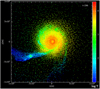 |
Fig. 7 State of the system after 24 h of simulation time. |
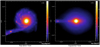 |
Fig. 8 Density rendering of the system after 24 h of simulation time. A disk-like structure can be seen around an almost spherical inner planet. The color rendering on the right-hand picture represents the column density. |
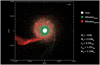 |
Fig. 9 Compositional analysis after 24 h of simulation time. Colors denote the different materials and origins. We can see a stream of material that is dominated by impactor material. Assuming no mass loss from the subsequent disk evolution we get an estimated Moon mass of Mm = 1.23MM. |
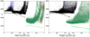 |
Fig. 10 Temperature profile of the multi-layered proto-Earth (left) and simple-layered proto-Earth (right) before and 24 h after impact. The gray (core) and light green (mantle) show the pre-impact proto-earth conditions. The black (iron) and dark green (silicate) show material from the target planet, while blue (iron) and red (silicate) show material from the impactor. This can be directly compared to the figure from Canup (2008b) which looks at the same ranges. Comparing to their results we can see that both of our pre-impact proto-Earths have a more continuous temperature profile (except at core mantle boundary). The silicate mantle is around the same temperature while our iron core is about 1000–2000K hotter. The most significant difference can be seen in the multi-layered case, where in the post-impact results there is significant mixing between the outer core material and impactor core, which is not present in the simple-layered case or in the work of Canup (2008b). This is due to the outer core being in a hotter state (molten) as the impactor core slams into it, which causes an increase in the temperature of the outer core material as the impactor material mixes with it. The temperature of the shocked impactor material reaches around 34 000 K at its peak for the multi-layered case and about 42 000K in the simple-layered case. |
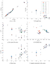 |
Fig. 11 Simulation results (those from Table 1). The size of the symbols represents the angular momentum of the impact. The colors represent different resolutions and whether the PES or PEM model were used: the blue and redrepresent the low-resolution PES and PEM models, while the green and purple represent the high-resolution PES and PEM model. The gradient in color represents the estimated mass of the Moon relative to the distribution. Surrounding gray borders represent cases that have more than 10% iron in their disk. Circles represent collisions made with a multi-layered proto-Earth and a rocky impactor, diamonds represent collisions made with a multi-layered proto-Earth and an icy impactor, and squares represent collisions made with a simple-layered proto-Earth and a rocky impactor. Panel a: linear relationship between the mass and angular momentum of the disk. Panel b: increase in escaped mass as the impact parameter decreases, which is because of the higher impact velocity required to recreate the given Limp. From panel c we can see, in general, a high negative disk–planet deviation as we increase the impact parameter. Panel d: shows that Q values for all the simulations are within the realistic limits (0 < Qimp < 5). Panels e and f: show that most prominent impacts occur in the range of 0.7 < b < 0.76. |
System properties of the fast-spinning simulations.
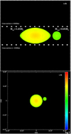 |
Fig. 12 Initial setup of the Lrf12Molten simulation.The impact parameter, impact velocity, and spin of the target planet is in this case set to b = − 0.3, vimp = 20 km s−1 and Ptar = 2.3 h respectively.The color rendering represents the temperature. Upper figure: equatorial view of the initial setup. The cross section that can be seen represents the region in which particles are rendered, which is done to improve the clarity of the following figures. Lower figure: top-down view of the initial setup and is the viewpoint in the upcoming figures. |
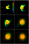 |
Fig. 13 Top-down view of the evolution of the collision of the Lrf12Molten simulation. The temperature range and spatial range can be seen in the top left panel. The times at which the images were taken, starting from the upper left, are t = 0.25, 1, 2, 5, 7.5, 12 h. |
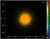 |
Fig. 14 State of the system after 24 h of simulation time. |
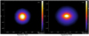 |
Fig. 15 Density rendering of the system after 24 h of simulation time. No real disk-like structure can be seen, the material appears evenly stratified around a fast-spinning inner core. The color rendering on the right picture represents the column density. |
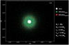 |
Fig. 16 Compositional analysis after 24 h of simulation time. Colors denote the different materials and origins. We can see that the target and impactor material are very evenly and isotropically distributed in the disk. Assuming no mass loss from the subsequent disk evolution we get an estimated Moon mass of Mm = 0.13MM. |
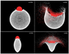 |
Fig. 17 Two snapshots from different viewing angles of the impactor penetrating into the target planet. Upper figure: top-down view and bottom figure: equatorial view. The impactor is fully rendered in red and only the surface particles of the target planet are rendered in white. Top panels: impactor making a large crater and reaching the core of the planet. Bottom figures: show that there are quite a lot of particles that scatter out from the plane of collision. |
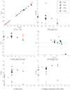 |
Fig. 18 Results from all the simulations in Table 2. The size of the symbols represents the impact velocity. The thickness of the surrounding black line represents the different initial spin periods, with the thickest being the 2.3 h case. The colors represent different proto-Earth models: the blue, red, green, and purple represent the PES, PEM, two-layered model, and the two-layered model with three times the vaporization energy respectively. The gradient in the color represents the estimated mass of the Moon relative to the distribution. The dashed lines in panel d represent the limits of the allowed compositional value of the impactor. The dashed line in panel f represents the angular momentum of the 2.3 h spinning planet. Panel a: linear relationship between the mass and angular momentum of the disk. Panel c: reveals that, in general, there is a small disk–planet deviation. Panel d: shows that most of the simulations result in unrealistic Q values whichare outside the limits (0 < Qimp < 5). Panels e and f: show that we cannot create a Moon-like satellite in this case. |
6 Conclusions
Our compositional analysis of the lunar-forming impact reveals that the classical models of a chemically uniform mantle are inconsistent with the current observed FeO/MgO difference between the Earth and the Moon. Either an additional source of enrichment is required or a Theia with near-identical Earth-like isotopic composition. An enstatite composition for Theia is still possible, but would require substantial mantle oxidation post-impact.
From our high-resolution canonical simulations we can conclude that a magma ocean of 300–500 km in depth slightly increases the mixing and results in a less massive Moon. The canonical simulations fit well withthe dynamical aspects of the Earth–Moon system, with an impact parameter of around b = 0.73 and angular momentum of around Limp = 1.25LEM. These simulations resulted in ahigh δfT value, whichmeans that we require a near Earth-like isotopic composition for Theia. These results agree well with the results from Canup (2004). The main trends are seen regardless of whether a multi-layered proto-Earth is used instead of a simple-layered proto-Earth. Although the simple-layered proto-Earth did in general produce smaller moon masses at a given impact angular momentum, we predict that this is mainly due to the increase in the radius of the simple-layered proto-Earth model, as the results were relatively sensitive to slight increases in the impact velocity. Using an icy Theia in the canonical model led to a higher δfT value and amore massive Moon compared to using a rocky Theia. The high δfT value makes this case very unlikely, as CI-chondrite requires a very low δfT value to be compatible with observations. In regard to the fast-spinning case, our simulations were not able to produce a sufficiently massive Moon.
Appendix A: Planetary models
Below are the models used in the simulations.
A.1 Proto-Earth models
Ic = Inner core Oc = Outer core Lm = Lower mantle Um = Upper mantle Mo = Molten ocean
PES Multi-layered Model 1 M = 1.05ME PC = 378 GPa TC = 5400 K.
PEM Multi-layered Model 1 M = 1.05ME PC = 385 GPa TC = 5400 K.
PES Two-layered Model 1 M = 1.05ME PC = 377 GPa TC = 5200 K.
PES Multi-layered Model 2 M = 0.95ME PC = 354 GPa TC = 5400 K.
PEM Multi-layered Model 2 M = 0.95ME PC = 361 GPa TC = 5400 K.
PES Simple-layered Model 2 M = 0.95ME PC = 354 GPa TC = 5400 K.
PEM Simple-layered Model 2 M = 0.95ME PC = 362 GPa TC = 5400 K.
A.2 Theia
Rocky Model 1 M = 0.05ME PC = 33.7 GPa TC = 1300 K.
Rocky model 2 M = 0.142ME PC = 71.9 GPa TC = 1800 K.
Icy model M = 0.142ME PC = 18.6 GPa TC = 500 K.
Appendix B: Shell distribution method
The numberof particles per shell is determined by the surrounding mass:
 (B.1)
(B.1)
Here, ri is not the position of the shells, but instead the mass boundaries that surround each shell. These boundaries go from r = 0 to r = R in which each mass boundary position is given by:
 (B.2)
(B.2)
where li determines the mass boundary distance. Each shell is placed halfway between each mass boundary:
 (B.3)
(B.3)
To determine the distance li between each mass boundary we begin first by calculating the mean particle distance in the current layer (inspired by Bobrick et al. 2017):
 (B.4)
(B.4)
Here, the l subscript represents the current layer, C is a constant, and  is the mean density of the layer. The number of shells in this layer is then given by:
 (B.5)
(B.5)
which is rounded to an integer number and then used to recalculate δl = rl∕n. This is acceptable for a one-layer planet or a layer with small density discontinuities. However, for planets with large density discontinuities we add one extra term to the equation:
 (B.6)
(B.6)
where K is a constant that is adjusted to fit with the SPH density approximation for the largest density drop in the planet max(Δρl). This was found to lead to good fits with any other density discontinuity found in the planet (Δρl). We can then use epsilon to once again recalculate δl.
 (B.7)
(B.7)
The length li is finally then given by:
 (B.8)
(B.8)
The “i” subscript represents the current shell. The constant C given above can be adjusted to give more or less shells.
Appendix C: Compositional analysis method
The compositional deviation from the Earth can be quantified using the ɛ notation:
 (C.1)
(C.1)
where Δ represents the ratio between two compositions and the subscript E signifies Earth values. The epsilon notation is usually used when measuring deviations in isotopic compositions and as these are usually quite small, the epsilon measures the relative deviation in parts of 104 and will thus have the limits [−∞ 104]. After a collision the deviation in composition of the resulting planet and Moon can be determined by two simple mass balance equations (Canup 2012):
 (C.2)
(C.2)
 (C.3)
(C.3)
where FP and FD represent the fraction of target material in the resulting planet and disk. ɛP, ɛM, ɛtar, ɛimp are the deviations of the resulting planet, Moon, target planet, and impactor. Assuming that the isotopic deviation is spread equally in the silicate material of the planet we can investigate the allowed values for ɛtar and ɛimp in a collision. This is because for the Earth-Theia collision the deviations of the resulting planet (Earth) and Moon is known. Setting ɛP = 0 and relating ɛtar ɛimp we can rewrite Eqs. (C.2) and (C.3) as:
 (C.4)
(C.4)
 (C.5)
(C.5)
 (C.6)
(C.6)
where δfT indicates the percentage of silicate material from the target planet in the resulting Earth and disk, and δfT = 0 represents a disk with an equal fraction of target material as in the resulting Earth. This allows one to investigate the allowed δfT percentages to give the seen isotopic variation between Earth and Moon for different kinds of impactor (Meier et al. 2014; Canup 2012).
We can develop a similar approach to decipher the effect of using a target with several silicate layers. However, for this we have to rewrite Eq. (C.2) in terms of the deviation in the different material layers of the target planets:
 (C.7)
(C.7)
where ɛtar,1 and ɛtar,n represent the deviation from the terrestrial value of the targets main and nth silicate material. FP,1 and FP,n are the mass fractions of the main and nth silicate material that comes from the target planet and ends up in the resulting planet. One can derive a similar expression for ɛM, which is written in terms of the different disk fractions instead:
 (C.8)
(C.8)
Setting ɛP = 0 and combining these equations leads to:
 (C.9)
(C.9)
Here we decide to dispatch of the epsilon notation and instead rewrite it in ratios as this gives a much clearer picture when dealing with large differences:
 (C.10)
 (C.11)
 (C.12)
Here Kn is the exchange function with respect to material 1:
 (C.13)
The equation then becomes:
 (C.14)
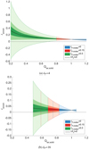 |
Fig. C.1 Result of the compositional analysis. The blue, red, and green areas indicate the cases in which the ratios of molten material in the resulting planet are δP,molten = 0, 0.15, 0.3, respectively.The vertical red and blue lines represent the extent of the red and blue areas. The light colors represent |δfT | < 40%, medium colors represent |δfT| < 13%, and dark colors represent |δfT| < 6%. The black dashed line highlights δenrich = 0 and the black solid line highlights |δfT| = 0. |
References
- Abe, Y. 1997, Phys. Earth Planet. Inter., 100, 27 [NASA ADS] [CrossRef] [Google Scholar]
- Agertz, O., Moore, B., Stadel, J., et al. 2007, MNRAS, 380, 963 [NASA ADS] [CrossRef] [Google Scholar]
- Asphaug, E., Collins, G., & Jutzi, M. 2015, Global Scale Impacts, eds. P. Michel, F. E. DeMeo, & W. F. Bottke (Tucson, AZ: University of Arizona Press), 661 [Google Scholar]
- Benz, W., Cameron, A. G. W., & Melosh, H. J. 1989, Icarus, 81, 113 [NASA ADS] [CrossRef] [Google Scholar]
- Bobrick, A., Davies, M. B., & Church, R. P. 2017, MNRAS, 467, 3556 [NASA ADS] [CrossRef] [Google Scholar]
- Cameron, A. G. W., & Ward, W. R. 1976, Lunar and Planetary Science Conference, 7 [Google Scholar]
- Canup, R. M. 2004, Icarus, 168, 433 [NASA ADS] [CrossRef] [Google Scholar]
- Canup, R. M. 2008a, Icarus, 196, 518 [NASA ADS] [CrossRef] [Google Scholar]
- Canup, R. M. 2008b, Lunar and Planetary Science Conference, 2429 [Google Scholar]
- Canup, R. M. 2012, Science, 338, 1052 [NASA ADS] [CrossRef] [Google Scholar]
- Canup, R. M., & Asphaug, E. 2001, Nature, 412, 708 [NASA ADS] [CrossRef] [Google Scholar]
- Costa, G. C. C., Jacobson, N. S., & Fegley, Jr. B. 2017, Icarus, 289, 42 [CrossRef] [Google Scholar]
- Ćuk, M., & Stewart, S. T. 2012, Science, 338, 1047 [NASA ADS] [CrossRef] [Google Scholar]
- Dauphas, N. 2017, Nature, 541, 521 [NASA ADS] [CrossRef] [Google Scholar]
- Dehnen, W., & Aly, H. 2012, MNRAS, 425, 1068 [NASA ADS] [CrossRef] [Google Scholar]
- Gingold, R. A., & Monaghan, J. J. 1977, MNRAS, 181, 375 [Google Scholar]
- Goldreich, P., Lithwick, Y., & Sari, R. 2004, ApJ, 614, 497 [NASA ADS] [CrossRef] [Google Scholar]
- Hartmann, W. K., & Davis, D. R. 1975, Icarus, 24, 504 [NASA ADS] [CrossRef] [Google Scholar]
- Herwartz, D., Pack, A., Friedrichs, B., & Bischoff, A. 2014, Science, 344, 1146 [CrossRef] [Google Scholar]
- Hosono, N., Karato, S.-i., Makino, J., & Saitoh, T. R. 2019, Nat. Geosci., 12, 418 [CrossRef] [Google Scholar]
- Ida, S., & Makino, J. 1993, Icarus, 106, 210 [NASA ADS] [CrossRef] [MathSciNet] [Google Scholar]
- Ida, S., Canup, R. M., & Stewart, G. R. 1997, Nature, 389, 353 [NASA ADS] [CrossRef] [Google Scholar]
- Javoy, M. 1995, Geophys. Res. Lett., 22, 2219 [NASA ADS] [CrossRef] [Google Scholar]
- Jing, Z., & Karato, S.-i. 2011, Geochim. Cosmochim. Acta, 75, 6780 [CrossRef] [Google Scholar]
- Jones, J. H., & Palme, H. 2000, Origin of the Earth and Moon, eds. R. M. Canup, & K. Righter (Tucson, AZ: University of Arizona Press), 197 [Google Scholar]
- Kaib, N. A., & Cowan, N. B. 2015, Icarus, 252, 161 [NASA ADS] [CrossRef] [Google Scholar]
- Karato, S.-I. 2014, Proc. Jpn. Acad., Ser. B, 90, 97 [CrossRef] [Google Scholar]
- Kokubo, E., Ida, S., & Makino, J. 2000, Icarus, 148, 419 [CrossRef] [Google Scholar]
- Lock, S. J., & Stewart, S. T. 2017, J. Geophys. Res. Planets, 122, 950 [CrossRef] [Google Scholar]
- Lock, S. J., Stewart, S. T., Petaev, M. I., et al. 2018, J. Geophys. Res. Planets, 123, 910 [NASA ADS] [CrossRef] [Google Scholar]
- Lucy, L. B. 1977, AJ, 82, 1013 [NASA ADS] [CrossRef] [Google Scholar]
- Mastrobuono-Battisti, A., Perets, H. B., & Raymond, S. N. 2015, Nature, 520, 212 [CrossRef] [Google Scholar]
- McKinnon, W. B. 2008, Bull. Am. Astron. Soc., 40, 464 [Google Scholar]
- Meier, M. M. M., Reufer, A., & Wieler, R. 2014, Icarus, 242, 316 [CrossRef] [Google Scholar]
- Melosh, H. J. 2007, Meteorit. Planet. Sci., 42, 2079 [NASA ADS] [CrossRef] [Google Scholar]
- Melosh, H. J. 2009, Meteorit. Planet. Sci. Suppl., 72, 5104 [Google Scholar]
- Mibe, K., Fujii, T., Yasuda, A., & Ono, S. 2006, Geochim. Cosmochim. Acta, 70, 757 [CrossRef] [Google Scholar]
- Morris, J. P., & Monaghan, J. J. 1997, J. Comput. Phys., 136, 41 [NASA ADS] [CrossRef] [MathSciNet] [Google Scholar]
- Mosenfelder, J. L., Asimow, P. D., Frost, D. J., Rubie, D. C., & Ahrens, T. J. 2009, J. Geophys. Res. Solid Earth, 114, B01203 [NASA ADS] [CrossRef] [Google Scholar]
- Nakajima, M., & Stevenson, D. J. 2014, Icarus, 233, 259 [NASA ADS] [CrossRef] [Google Scholar]
- Pahlevan, K., & Stevenson, D. J. 2007, Earth Planet. Sci. Lett., 262, 438 [CrossRef] [Google Scholar]
- Pahlevan, K., Stevenson, D. J., & Eiler, J. M. 2011, Earth Planet. Sci. Lett., 301, 433 [NASA ADS] [CrossRef] [Google Scholar]
- Park, R. S., Konopliv, A. S., Bills, B. G., et al. 2016, Nature, 537, 515 [NASA ADS] [CrossRef] [Google Scholar]
- Price, D. J. 2007, PASA, 24, 159 [Google Scholar]
- Rasio, F. A., & Lombardi, Jr. J. C. 1999, J. Comput. Appl. Math., 109, 213 [CrossRef] [Google Scholar]
- Reinhardt, C.,& Stadel, J. 2017, MNRAS, 467, 4252 [NASA ADS] [CrossRef] [Google Scholar]
- Reufer, A., Meier, M. M. M., Benz, W., & Wieler, R. 2012, Icarus, 221, 296 [NASA ADS] [CrossRef] [Google Scholar]
- Saff, E. B., & Kuijlaars, A. B. J. 1997, Math. Intell., 19, 5 [CrossRef] [MathSciNet] [Google Scholar]
- Saitoh, T. R., & Makino, J. 2013, ApJ, 768, 44 [NASA ADS] [CrossRef] [Google Scholar]
- Sasaki, S., & Nakazawa, K. 1986, J. Geophys. Res., 91, 9231 [NASA ADS] [CrossRef] [Google Scholar]
- Stewart, S. T., Davies, E. J., Duncan, M. S., et al. 2019, ArXiv e-prints [arXiv:1910.04687] [Google Scholar]
- Stixrude, L., & Lithgow-Bertelloni, C. 2005, Geophys. J. Int., 162, 610 [NASA ADS] [CrossRef] [Google Scholar]
- Thomas, P. C., Parker, J. W., McFadden, L. A., et al. 2005, Nature, 437, 224 [NASA ADS] [CrossRef] [PubMed] [Google Scholar]
- Thomas, C. W., Liu, Q., Agee, C. B., Asimow, P. D., & Lange, R. A. 2012, J. Geophys. Res. Solid Earth, 117, B10206 [CrossRef] [Google Scholar]
- Thompson, S. L., & Lauson, H. S. 1972, Improvements in the Chart D Radiation-Hydrodynamic Code. III: Revised Analytic Equations of State, Tech.rep. [Google Scholar]
- Tillotson, J. H. 1962, General Atomic Report GA-3216 [Google Scholar]
- Touma, J., & Wisdom, J. 1998, AJ, 115, 1653 [NASA ADS] [CrossRef] [Google Scholar]
- Wade, J., & Wood, B. J. 2005, Earth Planet. Sci. Lett., 236, 78 [CrossRef] [Google Scholar]
- Walsh, K. J., Morbidelli, A., Raymond, S. N., O’Brien, D. P., & Mandell, A. M. 2011, Nature, 475, 206 [NASA ADS] [CrossRef] [PubMed] [Google Scholar]
- Warren, P. H. 2005, Meteorit. Planet. Sci., 40, 477 [CrossRef] [Google Scholar]
- Warren, P. H., & Dauphas, N. 2014, Lunar Planet. Sci. Conf., 45, 2298 [Google Scholar]
- Weppner, S. P., McKelvey, J. P., Thielen, K. D., & Zielinski, A. K. 2015, MNRAS, 452, 1375 [NASA ADS] [CrossRef] [Google Scholar]
- Wetzstein, M., Nelson, A. F., Naab, T., & Burkert, A. 2009, ApJS, 184, 298 [NASA ADS] [CrossRef] [Google Scholar]
- Wiechert, U., Halliday, A. N., Lee, D.-C., et al. 2001, Science, 294, 345 [CrossRef] [Google Scholar]
- Zhang, J., Dauphas, N., Davis, A. M., Leya, I., & Fedkin, A. 2012, Nat. Geosci., 5, 251 [CrossRef] [Google Scholar]
The spin period is approximate, specifically the spin of the planet is fitted to the angular momentum given in Ćuk & Stewart (2012).
It can be greater than LEM due to tidal interaction with the Sun. If the Moon was captured in evection resonance, the angular momentum could decrease by a factor of two (Ćuk & Stewart 2012).
To give a good correlation with the equatorial radius of the fast-spinning case, the gyration constant is set to 0.69.
All Tables
All Figures
|
Fig. 1 Depiction of the initial condition of the M = 1.05ME multi-layered PES model. Here, we show how the true density compares with the approximated density from the SPH summation formula. The initial SPH density is given from the initial distribution of particles using the method described in Appendix B. The density after relaxation is given by the green curve. We can see that in general we get a very good fit; however, we do get a slight a gap between the density discontinuities, which is characteristic of the artificial surface tension effect (Agertz et al. 2007). |
| In the text | |
|
Fig. 2 Top-down view of an impact, highlighting the important parameters involved in the collision. |
| In the text | |
|
Fig. 3 Result of the compositional analysis with δP = 8. The blue, red, and green areas represent the cases in which the ratios of molten material in the resulting planet are δP,molten = 0, 0.15, 0.3 respectively.The vertical red and blue lines represent the extent of the red and blue areas. The light colors represent |δfT | < 40%, medium colors represent |δfT| < 13%, and dark colors represent |δfT| < 6%. The black dashed line highlights δenrich = 0 and the black solid line highlights |δfT| = 0. |
| In the text | |
|
Fig. 4 Allowed values for the relative FeO/MgO of the target planet and impactor for different δP. The boundary line to the right of each shaded area represents δP,molten = 0 and the boundary line to the left represents δP,molten = 0.3. |
| In the text | |
|
Fig. 5 Initial setup of the Hrc1Solid simulation. The impact parameter and angular momentum are in this case set to b = 0.3 and Limp = 1.25LEM respectively.The color rendering represents the temperature. Upper figure: equatorial view of the initial setup. The cross section that can be seen represents the region in which particles are rendered, which is done to improve the clarity of the following figures. Lower panel: top-down view of the initial setup and is the viewpoint in the following figures. |
| In the text | |
|
Fig. 6 Top-down view of the evolution of the collision for the Hrc1Solid simulation. The temperature range and spatial range can be seen in the top left figure. The times when each of the images were captured, starting from the upper left, are t = 0.25, 1, 2, 5, 7.5, 12 h. |
| In the text | |
|
Fig. 7 State of the system after 24 h of simulation time. |
| In the text | |
|
Fig. 8 Density rendering of the system after 24 h of simulation time. A disk-like structure can be seen around an almost spherical inner planet. The color rendering on the right-hand picture represents the column density. |
| In the text | |
|
Fig. 9 Compositional analysis after 24 h of simulation time. Colors denote the different materials and origins. We can see a stream of material that is dominated by impactor material. Assuming no mass loss from the subsequent disk evolution we get an estimated Moon mass of Mm = 1.23MM. |
| In the text | |
|
Fig. 10 Temperature profile of the multi-layered proto-Earth (left) and simple-layered proto-Earth (right) before and 24 h after impact. The gray (core) and light green (mantle) show the pre-impact proto-earth conditions. The black (iron) and dark green (silicate) show material from the target planet, while blue (iron) and red (silicate) show material from the impactor. This can be directly compared to the figure from Canup (2008b) which looks at the same ranges. Comparing to their results we can see that both of our pre-impact proto-Earths have a more continuous temperature profile (except at core mantle boundary). The silicate mantle is around the same temperature while our iron core is about 1000–2000K hotter. The most significant difference can be seen in the multi-layered case, where in the post-impact results there is significant mixing between the outer core material and impactor core, which is not present in the simple-layered case or in the work of Canup (2008b). This is due to the outer core being in a hotter state (molten) as the impactor core slams into it, which causes an increase in the temperature of the outer core material as the impactor material mixes with it. The temperature of the shocked impactor material reaches around 34 000 K at its peak for the multi-layered case and about 42 000K in the simple-layered case. |
| In the text | |
|
Fig. 11 Simulation results (those from Table 1). The size of the symbols represents the angular momentum of the impact. The colors represent different resolutions and whether the PES or PEM model were used: the blue and redrepresent the low-resolution PES and PEM models, while the green and purple represent the high-resolution PES and PEM model. The gradient in color represents the estimated mass of the Moon relative to the distribution. Surrounding gray borders represent cases that have more than 10% iron in their disk. Circles represent collisions made with a multi-layered proto-Earth and a rocky impactor, diamonds represent collisions made with a multi-layered proto-Earth and an icy impactor, and squares represent collisions made with a simple-layered proto-Earth and a rocky impactor. Panel a: linear relationship between the mass and angular momentum of the disk. Panel b: increase in escaped mass as the impact parameter decreases, which is because of the higher impact velocity required to recreate the given Limp. From panel c we can see, in general, a high negative disk–planet deviation as we increase the impact parameter. Panel d: shows that Q values for all the simulations are within the realistic limits (0 < Qimp < 5). Panels e and f: show that most prominent impacts occur in the range of 0.7 < b < 0.76. |
| In the text | |
|
Fig. 12 Initial setup of the Lrf12Molten simulation.The impact parameter, impact velocity, and spin of the target planet is in this case set to b = − 0.3, vimp = 20 km s−1 and Ptar = 2.3 h respectively.The color rendering represents the temperature. Upper figure: equatorial view of the initial setup. The cross section that can be seen represents the region in which particles are rendered, which is done to improve the clarity of the following figures. Lower figure: top-down view of the initial setup and is the viewpoint in the upcoming figures. |
| In the text | |
|
Fig. 13 Top-down view of the evolution of the collision of the Lrf12Molten simulation. The temperature range and spatial range can be seen in the top left panel. The times at which the images were taken, starting from the upper left, are t = 0.25, 1, 2, 5, 7.5, 12 h. |
| In the text | |
|
Fig. 14 State of the system after 24 h of simulation time. |
| In the text | |
|
Fig. 15 Density rendering of the system after 24 h of simulation time. No real disk-like structure can be seen, the material appears evenly stratified around a fast-spinning inner core. The color rendering on the right picture represents the column density. |
| In the text | |
|
Fig. 16 Compositional analysis after 24 h of simulation time. Colors denote the different materials and origins. We can see that the target and impactor material are very evenly and isotropically distributed in the disk. Assuming no mass loss from the subsequent disk evolution we get an estimated Moon mass of Mm = 0.13MM. |
| In the text | |
|
Fig. 17 Two snapshots from different viewing angles of the impactor penetrating into the target planet. Upper figure: top-down view and bottom figure: equatorial view. The impactor is fully rendered in red and only the surface particles of the target planet are rendered in white. Top panels: impactor making a large crater and reaching the core of the planet. Bottom figures: show that there are quite a lot of particles that scatter out from the plane of collision. |
| In the text | |
|
Fig. 18 Results from all the simulations in Table 2. The size of the symbols represents the impact velocity. The thickness of the surrounding black line represents the different initial spin periods, with the thickest being the 2.3 h case. The colors represent different proto-Earth models: the blue, red, green, and purple represent the PES, PEM, two-layered model, and the two-layered model with three times the vaporization energy respectively. The gradient in the color represents the estimated mass of the Moon relative to the distribution. The dashed lines in panel d represent the limits of the allowed compositional value of the impactor. The dashed line in panel f represents the angular momentum of the 2.3 h spinning planet. Panel a: linear relationship between the mass and angular momentum of the disk. Panel c: reveals that, in general, there is a small disk–planet deviation. Panel d: shows that most of the simulations result in unrealistic Q values whichare outside the limits (0 < Qimp < 5). Panels e and f: show that we cannot create a Moon-like satellite in this case. |
| In the text | |
|
Fig. C.1 Result of the compositional analysis. The blue, red, and green areas indicate the cases in which the ratios of molten material in the resulting planet are δP,molten = 0, 0.15, 0.3, respectively.The vertical red and blue lines represent the extent of the red and blue areas. The light colors represent |δfT | < 40%, medium colors represent |δfT| < 13%, and dark colors represent |δfT| < 6%. The black dashed line highlights δenrich = 0 and the black solid line highlights |δfT| = 0. |
| In the text | |
Current usage metrics show cumulative count of Article Views (full-text article views including HTML views, PDF and ePub downloads, according to the available data) and Abstracts Views on Vision4Press platform.
Data correspond to usage on the plateform after 2015. The current usage metrics is available 48-96 hours after online publication and is updated daily on week days.
Initial download of the metrics may take a while.