| Issue |
A&A
Volume 642, October 2020
|
|
|---|---|---|
| Article Number | A43 | |
| Number of page(s) | 12 | |
| Section | Planets and planetary systems | |
| DOI | https://doi.org/10.1051/0004-6361/202038592 | |
| Published online | 02 October 2020 | |
A charging model for the Rosetta spacecraft
1
Swedish Institute of Space Physics,
Uppsala,
Sweden
e-mail: This email address is being protected from spambots. You need JavaScript enabled to view it.
2
Uppsala University, Department of Astronomy and Space Physics,
Uppsala, Sweden
3
Laboratoire de Physique et Chimie de l’Environnement et de l’Espace, CNRS,
Orléans, France
4
Laboratoire Lagrange, OCA, CNRS, UCA,
Nice, France
5
University Paul Sabatier Toulouse III,
Toulouse, France
6
ESA/ESTEC,
Noordwijk, The Netherlands
7
Airbus Defence and Space GmbH,
Friedrichshafen, Germany
Received:
5
June
2020
Accepted:
6
August
2020
Abstract
Context. The electrostatic potential of a spacecraft, VS, is important for the capabilities of in situ plasma measurements. Rosetta has been found to be negatively charged during most of the comet mission and even more so in denser plasmas.
Aims. Our goal is to investigate how the negative VS correlates with electron density and temperature and to understand the physics of the observed correlation.
Methods. We applied full mission comparative statistics of VS, electron temperature, and electron density to establish VS dependence on cold and warm plasma density and electron temperature. We also used Spacecraft-Plasma Interaction System (SPIS) simulations and an analytical vacuum model to investigate if positively biased elements covering a fraction of the solar array surface can explain the observed correlations.
Results. Here, the VS was found to depend more on electron density, particularly with regard to the cold part of the electrons, and less on electron temperature than was expected for the high flux of thermal (cometary) ionospheric electrons. This behaviour was reproduced by an analytical model which is consistent with numerical simulations.
Conclusions. Rosetta is negatively driven mainly by positively biased elements on the borders of the front side of the solar panels as these can efficiently collect cold plasma electrons. Biased elements distributed elsewhere on the front side of the panels are less efficient at collecting electrons apart from locally produced electrons (photoelectrons). To avoid significant charging, future spacecraft may minimise the area of exposed bias conductors or use a positive ground power system.
Key words: plasmas / comets: individual: 67P/Churyumov-Gerasimenko / methods: numerical / methods: data analysis / space vehicles
© ESO 2020
1 Introduction
The European Space Agency’s (ESA) comet chaser, Rosetta, monitored the plasma environment of comet 67P/Churyumov-Gerasimenko from August 2014 to September 2016. The scientific payload included the Rosetta Plasma Consortium (RPC, Carr et al. 2007), dedicated to understanding the composition and evolution of the comet plasma. The RPC included, among other instruments, the Langmuir probe (LAP, Eriksson et al. 2007, 2017) and the Mutual Impedance Probe (MIP, Trotignon et al. 2007; Henri et al. 2017). Because the instruments are mounted on Rosetta, the RPC observations of charged particles are influenced by the electrostatic potential of the spacecraft with respect to its environment, VS, but several RPC measurements can also be used to quantify this potential.
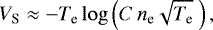
All objects in space exchange charge with their surroundings, mainly due to the collection of charged particles impacting the object and emission of electrons via the photoelectric effect and secondary emission. There are about as many negative electrons as positive ions in a plasma, but the electrons usually move much faster. In consequence, more electrons than ions tend to hit an uncharged spacecraft, giving it a negative charge unless the plasma is so tenuous that photoelectron emission dominates. An equilibrium is reached when the spacecraft becomes so negative that most plasma electrons are repelled. When the dominating compensating current is photoelectron emission, the spacecraft potential VS of a conductive spacecraft becomes (Odelstad et al. 2017)
 (1)
(1)
where ne is the number density the electrons, which are assumed to be a Maxwellian population of characteristic temperature Te, given in eV, and C is a constant not depending on the plasma properties. The quantity in the logarithm essentially is the electron flux, which, together with Te is thus expected to drive the VS in this case. If the collection of ions is a significant contribution to the current, the dependence on density becomes weaker.
Predictions for the spacecraft potential of Rosetta had already been produced prior to launch. In two coupled studies, Roussel & Berthelier (2004) used numerical simulations and Berthelier & Roussel (2004) investigated a spacecraft model in a laboratory plasma. Several plasma cases, including fully cooled (0.005 eV) cometary electrons were considered in the numerical simulations. Some simulations let the solar arrays to float into their own equilibrium potential which was found to be beneficial for reducing the otherwise often several volts positive potential observed in the simulations. The laboratory studies, therefore, emulated this case, with different surfaces on the model spacecraft insulated from each other and thus attaining their own equilibrium. The studies, which did not include biased elements on the solar arrays, suggested Rosetta would attain potentials between a few times − kBTe∕e and about + 10 V.
However, the spacecraft potential was continuously measured by LAP and found to be negative during most of the of Rosetta cometary operations (Odelstad et al. 2015, 2017). The spacecraft often reached negative potentials around and in excess of −15 V, which have a severe effect on in situ measurements of the plasma environment surrounding the spacecraft as electrons are repelled (Eriksson et al. 2017) and positive ions are perturbed (Bergman et al. 2019, 2020). From this spacecraft potential result, Odelstad et al. (2017), with Eq. (1), argued that the component dominating the electron flux is a thermal ≈ 5− 10 eV population omnipresent in the parts of the comet coma visited by Rosetta. The existence of these warm electrons has also been verified by direct observation, by LAP (Eriksson et al. 2017), by MIP (Wattieaux et al. 2020), as well as by the RPC Ion and Electron Sensor (Broiles et al. 2016). However, there is also evidence of a highly variable cold (≲ 0.1 eV) population of electrons, independently detected by LAP (Eriksson et al. 2017; Engelhardt et al. 2018) and MIP (Gilet et al. 2019; Wattieaux et al. 2020).
The cold electron population accounted for a significant, sometimes dominant, part of the total the electron density from January to September 2016 (Wattieaux et al. 2020), but due to its low temperature, the cold electron flux is low and is not expected to drive the spacecraft potential. However, in our analysis of LAP and MIP data during the cross-calibration activities for the final data deliveries for the ESA Planetary Science Archive, we came to notice a strong correlation between total plasma density, including the cold population and the spacecraft potential. Here, we report on these findings and present our investigation into why this is the case.
We structure this paper as follows: in Sect. 2, we present new statistics of simultaneously measured electron temperature, density, and spacecraft potential data showing unexpected correlations. To explain the results, we investigate details of the Rosetta electrostatic design in Sect. 3 and present a series of particle in cell simulations of a simplified model dealing with exposed biased elements on the spacecraft solar array in Sect. 4 and discuss this model’s shortcomings and merits. To improve our model, we adapt an analytical model of the vacuum potential of a charged disk in Sect. 5 and run numerical simulations (Sect. 6) of a concentric disks geometry in an effort to highlight spacecraft design decisions with a critical influence on the cold electron current collection. Finally, we suggest a simplified model describing the Rosetta current balance by setting up a system of equations to describe the current to the spacecraft and a positively biased surface behind a negative potential barrier in Sect. 7, solve it numerically, and compare it to Rosetta results.
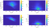 |
Fig. 1 2D histogram in 80 × 100 bins of 88 000 events of simultaneously measured spacecraft potential versus electron density (left column) and temperature (right column) from January to September 2016 at 2 to 3.8 AU. The identified electron populations by MIP from Wattieaux et al. (2020) are separated by temperature as warm (Tew ≈ 4 eV, top row) andcold (Tec ≈ 0.1 eV, bottom row).In total, 9700 outliers with either Tew > 15 eV (9400 outliers) or Tec > 0.5 eV (2800 outliers) have been removed. |
2 Data analysis
A reworked analysis of MIP spectra with signatures of two electron populations (Wattieaux et al. 2019; Gilet et al. 2019) yields an unprecedented precision in both energy and density of the thermal (≈ 5 eV) and cold (≈0.1 eV) electron populations. These estimates, combined with the recently published and improved spacecraft potential estimates from LAP (largely based on measurements published in Odelstad et al. 2017) in AMDA1, give us simultaneous measurements of all parameters in Eq. (1) for both populations. We plot the MIP density estimates, as well as the mean of the LAP spacecraft potential estimates (typically 1 or 29 samples) taken during the acquisition period of each MIP spectra (typically 2 s) and plot them in Fig. 1.
In contrast to our model in Eq. (1), the temperature variation in the two detected electron populations can only explain some of the variations in the Rosetta spacecraft potential. Instead, the cold electron density has the clearest (logarithmic) relation to spacecraft potential out of the four parameters investigated. However, for a uniformly charged spacecraft at −10 V, these cold (0.1 eV) electrons simply cannot reach the spacecraft and meaningfully contribute to the current balance that dictates the spacecraft potential.
The correlation between the cold electron density and the spacecraft potential is perhaps the clearest in a time-series, as plotted in Fig. 2 (top), where we also observe a rather weak dependence on warm electron density to spacecraft potential. We also note that from 2016-06-12T16:00:00 to 2016-06-13T08:00:00, the average temperature of plasma electrons should increase (up to 50 percent) as the cold electron population density decreases, which according to our relation in Eq. (1) would correspond to a more negative spacecraft potential. Instead, the opposite is true.
Normalising the spacecraft potential by e∕Tew in Fig. 2 (middle panel) we see that an increase in warm electron density (for a fixed Tew does not drive the spacecraft more negative at all during the entire period from January to September 2016. Instead, it seems that an increase in new is associated with a decrease of Tew, which is much more strongly coupled to the spacecraft potential. In general, it should not be surprising that in denser regions of the cometary ionosphere, the denser neutral cometary gas allows for more efficient cooling of all electrons (Edberg et al. 2015). What is also apparent is that the warm electron density does not strongly correlate with the cold electron density (bottom panel, same figure), which (albeit with more scatter) still shows the same trend of linearly increased charging with an exponential increase of cold electron density.
In the following section, we propose a mechanism to explain these observations.
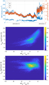 |
Fig. 2 Top: example time series of LAP spacecraft potential (diamonds), cold (circles), and warm (pluses) electron density estimates from MIP in the same interval, exhibiting the strong correlation between spacecraft potential and cold electron density. Middle: same data as shown in Fig. 1, 2D histogram of 120 × 150 bins of new vs. eVS ∕Tew. Bottom: as above, but with nec on the y-axis. |
3 Exploring what drives Rosetta to negative
Ionospheric spacecraft have been observed to be driven negative by exposed, positively biased conductors on solar panels. For example, the OGO-6 satellite was observed to reach about −20 V (Zuccaro & Holt 1982) and the International Space Station can reach as much as −140 V (Carruth et al. 2001). The reason is that such biased elements can draw a large electron current. To close the circuit, the spacecraft must respond by decreasing its potential to deflect more electrons away from it and to attract more ions from the plasma. This phenomenon can be regularly observed on small spacecraft equipped with Langmuir probes, where a large positive bias on the probe can result in a small negative shift of VS (e.g. Ivchenko et al. 2001). On Rosetta, the surface area of about 80 cm2 of each of the two LAP probes is negligibly small compared to the total spacecraft area (including solar panels) around 150 m2, so these cannot drive VS to the high negative values observed.
Rosetta was not expected to be (and effectively never was) exposed to the large fluxes of high energy particles often driving spacecraft charging to dangerous levels in, for example, auroral zones (Eriksson & Wahlund 2006; Garrett et al. 2008). Efforts were taken, nonetheless, to minimise exposed dielectrics and non-grounded conductors in order to provide a stable ground for plasma measurements. Providing a conductive and grounded outer layer was straightforward for most parts of the spacecraft. As Rosetta was to be the first spacecraft operating on only solar power as far from the Sun as 5.25 AU, the front side of the large (64 m2) solar arrays was a more complex issue, but in the end, it was decided that the solar cells would also be provided with cover glasses with a conductive indium tin oxide surface layer connected to spacecraft ground. In the low-energy dominated environments of concern here, the charging of dielectrics is not the primary concern. More of interest are exposed conductors, which can draw a significant current and, hence, influence the spacecraft potential. Thanks to the solar cell cover glasses and the equally conductive and grounded multi-layer insulation on the spacecraft body, the dominant fraction of all exposed conductive surfaces (we estimate at least 95%) is at spacecraft potential. However, there are exceptions, particularly on the solar panels.
The Rosetta solar array (Fig. 3) consists of 10 panels, each with 25 strings of 91 solar cells on its front side. While each cell has a conductive and grounded cover glass, there are small exposed biased conductors (interconnects) linking the cells in a string as well as the ends of a string to the spacecraft power bus. The single largest exposed positive potentials on a panel are the 25 small anodes of the bus bars at the end of each string, which can be seen as a sketch in Fig. 4. The bus bar anode is biased up to +79 V from spacecraft ground (and the bus bar cathode) on a string in open-circuit condition, and +65 V for a string operating at the maximum power point2. The 89 interconnects in each string between the anode and cathode are therefore biased to an equidistant and linearly increasing potential foreach consecutive solar cell in the string, such that the bias voltage on the last interconnect before a +79 V anode is +78.12 V, and the second to last is +77.24 V and so on. The bus bars are scattered on the panel, immediately surrounded by solar cells that are covered by a cover glass connected to spacecraft ground. The interconnects are more numerous but slightly smaller. Most of them are also scattered over the surface, but as each solar panel is organised into a grid of 57 rows and 42 columns, a string does not fit into one single column and so, it must wrap around when reaching a panel edge and continue along the next column. The upper and lower border of each solar panel front side are therefore lined by solar cell interconnects, and, as such, they are all biased to voltages between 0.7 and +78.12 V, depending on the bus bar anode potential. A naïve assumption might be to assume that incident electrons of any temperature could be collected at these voltages for the entire range of spacecraft potential measured inFig. 1 and, in some sense, eliminate the temperature dependence in Eq. (1).
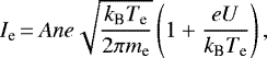
Based on simple Orbital-Motion Limited (OML) considerations, we see that small surfaces that are biased from the ground with a potential VB can easily dominate the positive current collection to a spacecraft as the current increases as a function of the absolute potential of the surface for any surface except an infinite plane (Laframboise & Parker 1973). For the simplest two-body problem of a spherical, positively charged body of surface area, A, immersed in a plasma of density, n, the current collection of electrons is
 (2)
(2)
where U is the absolute (positive) potential of the body U = VB + VS and other constants have their usual meaning. For 0.1 eV electrons and an exposed conductor at +75 V as discussed in the previous section, the current collection thus is leveraged by a factor of 750. Of course, charged elements on a spacecraft is a much more involved circuitry with a complex geometry that needs to be taken into account and requires numerical simulations.
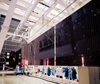 |
Fig. 3 Rosetta spacecraft and one of its solar wings. The solar cell cover glass on each cell is visible as small dark glossy surfaces, with metallic reflective interconnects above and below it. There are also 25 slightly larger reflective bus bar pairs, not to be confused with the six circular Kevlar cutter/hold-down points. Adapted from Rosetta Solar panels on ESA’s website. Retrieved May 4, 2020, from sci.esa.int/s/w0e6nbW. Copyright 2012 ESA-A, Van der Geest. Reprinted with permission. |
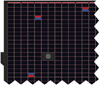 |
Fig. 4 Artistimpression of a corner section of the front side of a solar panel on Rosetta. The black squares are individual solar cells covered with grounded cover glass, connected in series via (pink) interconnects in a column that wrap around to the next column near the top edge (and bottom, not shown) of the solar panel via a longer interconnect (also pink). At the start and end of each string of 91 solar cells are bus bars, marked with red (anode) and blue (cathode). The grey circle represents one of six circular Kevlar cutter/hold-down points. All surfaces coloured in pink and red are exposed positively biased conductors. |
4 Numerical simulations
The Spacecraft-Plasma Interaction System (SPIS) is a hybrid code package to simulate the spacecraft-plasma interaction, solving the Gauss’s Law for electric fields, pushing particles, and simulating the spacecraft circuitry response and interaction with the plasma (Matéo-Vélez et al. 2012, 2015; Sarrailh et al. 2015). This work is a continuation of efforts of modelling the Rosetta spacecraft in a cometary plasma environment by Johansson et al. (2016) and Bergman et al. (2020) to understand the RPC instrument measurements. The simulation parameters for a reference simulation are provided in Table 1. The cometary ion population provides little current to the spacecraft system but ensures quasi-neutrality with a realistic (Stenberg Wieser et al. 2017) but isotropic thermal velocity. To reduce the computational time of some of the SPIS simulations, we can simulate particles also as a Maxwell-Boltzmann fluid approximation instead of a full particle-in-cell (PIC) simulation. This treatment is not valid when there are positively biased elements present as the electron density in each simulation cell is extrapolated from the potential in that cell and, as such, we would overestimate the electron density near positive elements and within potential barriers. However, the reduction of computational (PIC) noise from a fluid approximation is very welcome for the purposes of demonstration.
We can also gain insights by studying simplified geometries; given the solar panels are the largest areas, we neglect the body and becauseeach solar panel is large compared to the Debye length (which should be 30 cm or less with cold electrons around), the whole array should essentially behave as a single solar panel. Therefore, we approximate Rosetta with a box of size 1.25 × 1.25 × 0.15 m, where the thickness is exaggerated for the ease of simulation but brings in only a negligible contribution to the current balance. We also include four 0.1 × 0.1 m symmetrically placed elements on the front side of the solar panel, which we set to a bias potential VB = 75 V, as shown in Fig. 5. All surfaces are simulated as indium tin oxide (ITO) for the purpose of photoemission and conductivity as it is the principal material on all sunlit surfaces on Rosetta and we otherwise assume this to have a negligible effect on VS in a cometary (low-energy) plasma environment.
In Fig. 5, we show an instructive example of the potential structure around a −25 V solar panel with small positively biased elements from a SPIS simulation with with the electron density set by a Boltzmann relation with the potential, complete with a three-dimensional potential barrier of −8 V. As can be seen in Fig. 6, the effect of positively biased surfaces is two-fold:
-
The positively biased elements are collecting locally produced photoelectrons from the surrounding surfaces as well, where the current magnitude as measured by SPIS corresponds to the photosaturation current of an area six times their size. Effectively, this turns photoemission off on an area six times as large as the positively biased elements on the solararray and drives the spacecraft potential to be more negative. For a more realistic case, with exposed biased elementsthat are spread over the entire (sunlit) panel, the photoemission of Rosetta would be heavily suppressed. This can be part of the explanation on why Rosetta was substantially negatively charged during the cometary mission and readily explains why Rosetta only experienced moderate positive charging in the solar wind (Odelstad et al. 2017).
-
For standard OML, and indeed in the example SPIS Maxwell-Boltzmann fluid treatments in Figs. 5 and 6, the current to any positively charged surface (for the barrier potential, UM) is severely exaggerated as most electrons born at a potential of 0 V at infinity cannot penetrate the barrier if their energy does not exceed eUM. The aforementioned cold cometary electrons would contribute little to the current to these biased elements, as has indeed been confirmed by SPIS simulations with a PIC treatment of electrons.
This potential barrier effect is very effective in quenching the cold electron current when small positive elements are surrounded on all sides by grounded (negative) elements. Although the cold electron density population exhibits the exact behaviour we sought for in Sect. 2 in the fluid approximation simulations, we must look for another explanation when a realistic treatment of electrons is applied.
As described in Sect. 3 and in Fig. 4, the interconnects are dispersed all over the solar panel surfaces, but they are (possibly crucially) always present at the top and bottom border of the solar panel front side, as the solar cell string wraps around to the next column. As for all interconnects on the solar array, on average, this border is expected to be biased between +30 and 40 V (although an average may not be the best descriptor for the net effect on current collection since many interconnects would be repelling electrons exponentially at VB < −VS) and can have less restricted access to electrons as it is not surrounded by negatively charged surfaces, an effect we investigate further in the following sections.
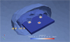 |
Fig. 5 Visualisation of electrostatic potential struture from a SPIS simulation of a model with four 0.1 × 0.1 m +75V biasedelements on a 1.25 × 1.25 × 0.15 m solar panel inside a spherical simulation volume of radius 15 m. Ten equipotential surfaces (cut in the Y = Z plane) from −17 V to +42.5 V are also plotted with the −8 V and −17 V surfaces specifically labelled. |
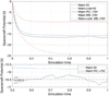 |
Fig. 6 Top: spacecraft (ground) potential evolution in five SPIS simulations. The reference simulation with no biased surfaces in a warm Tew = 10 eV plasma (blue line), with small charged surfaces of +75 V in a PIC simulation (black) or a fluid Maxwell-boltzmann simulation (yellow dot-dashed line). Also plotted, a simulation of the same plasma density but with 50 percent Tec = 0.1 eV electrons with either no biased surfaces (red), or with biased surfaces using the fluid approximation (purple dot-dash line). The Maxwell-Boltzmann simulations with surfaces at +75 V are strictly not valid but serve to illustrate the first approximation from Orbital-Motion-Limited theory. Bottom: zoom-in of above, with the calculated mean (dashed black line) and a 1σ range (dotted black lines) of spacecraft potential from the PIC simulation in this interval. |
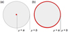 |
Fig. 7 Geometry of the concentric disk model for modelling of solar panels with biased elements as described in Sect. 5.1 for two different applications. Panel a: single exposed biased conductor on the main area of the solar panel (Sect. 5.2); panel b: exposes biased conductors along the edge (Sect. 5.3). Grey areas represent the main solar panel at spacecraft potential, red a biased element. |
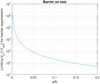 |
Fig. 8 Limiting potential ratio for barrier suppression for a small biased element on the z axis as given by Eq. (7). |
5 Analytical model of solar panels with biased elements
5.1 Vacuum model for thin circular disk
For a comparison and interpretation of the simulation results on the formation of potential barriers, we use an analytical solution of the Laplace equation around a thin circular disk which consists of two concentric parts, as illustrated by two examples in Fig. 7, an inner disc of radius, a, at potential, Vin, surrounded by an annulus of inner radius, a, and outer radius, b > a, at the potential Vout. At cylinder coordinates (ρ, ϕ, z), where z = 0 defines the disc plane, Sherman & Parker (1971) found that the vacuum potential from this object is
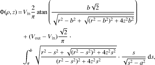 (3)
(3)
where r2 = ρ2 + z2. The integral can be analytically evaluated on the z axis and in the disk plane z = 0 to find that
![Mathematical equation: \begin{align} \Phi(0,z) &\,{=}\,\frac{2}{\pi} \left[ V_{\textrm{in}} \, \mathrm{atan} \frac{b}{z} + (V_{\textrm{out}}-V_{\textrm{in}}) \frac{z}{\sqrt{z^2+a^2}} \, \mathrm{atan} \sqrt{\frac{b^2-a^2}{z^2+a^2}}\ \right],\\ \Phi(\rho,0) &\,{=}\,\frac{2}{\pi} \left[ V_{\textrm{in}} \, \mathrm{atan} \frac{b}{\sqrt{\rho^2-b^2}} + (V_{\textrm{out}}-V_{\textrm{in}}) \, \mathrm{atan} \sqrt{\frac{b^2-a^2}{\rho^2-b^2}}\ \right].\end{align}](/articles/aa/full_html/2020/10/aa38592-20/aa38592-20-eq4.png)
We use these expressions to model potential barriers around solar panels with exposed biased conductors in Sects. 5.2 and 5.3 below. In extending an argument used by Sherman & Parker (1971) for the z axis, the potential will have an extremum (minimum or maximum) on exactly one of the two axes. This is because at large distance the two plates look like a point with charge equal to their net charge, which must be either positive or negative. Far away, the potential decays as ± 1∕r, so if negative at large distance, the potential must have a minimum somewhere along the axis from the positively charged part, which is the z axis if the positive part is the inner disk ρ < a and otherwise the ρ axis. Such a minimum in the potential is a maximum in electron potential energy and, hence, a potential barrier. By considering the net charge of the disks, the limit for barrier formation is found to be (Sherman & Parker 1971):
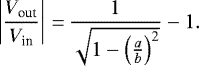 (6)
(6)
If the positive voltage, whether Vin as in Fig. 7a or Vout as in Fig. 7b, is higher than allowed by this expression, there will be no barrier for electron collection by the positive element.
5.2 Biased element in the centre of a solar panel
In this case, the outer annulus represents the solar panel at potential Vout = VS < 0 and the inner disk represents the biased element at Vin = VS + VB. The minimum value of Vin to break thebarrier follows from Eq. (6) as
 (7)
(7)
Figure 8 shows this expression evaluated for a range of the radial ratio a∕b. It is clear from this plot that forbiddingly large values of the bias ratio are needed for breaking the barrier, reinforcing the conclusion in Sect. 4 that small positive elements on the interior of a solar panel would not collect cold plasma electrons.
In Fig. 9, we show the vacuum electrostatic field near the centre of the same disk as calculated from the full expression Eq. (3) for four different bias voltages VB = Vin − Vout. The zero volt equipotential (red) ends at the intersection ρ = a = 0.02 b between the disks. All field lines starting on the positively biased inner surface ends up on the main solar panel area, as is expected since there is a potential barrier. The radius ρ0 delimiting field lines connecting to the inner disk or to infinity can be seen to expand from about 0.12 b to 0.18 b as VB increases from 30 V to 75 V. If photoelectrons were massless and emitted from the solar panel in the normal direction with zero speed, they would follow the electric field lines. Using ρ0 as a measure of the region from which photoelectrons from the solar panel would be collected by the biased element at the centre, we find that the area of this region is about 35 times bigger than the biased element itself already for VB = 30 V. While parameters are not perfectly comparable, this is still significantly more than the factor of about six that we found in the simulations in Sect. 4. This is expected, as photoelectrons would follow field lines perfectly only if massless and emitted at zero speed, neither of which is the case. Furthermore, our analytic model only considers a vacuum.
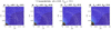 |
Fig. 9 Vacuum potential and electric field pattern in the ρ−z plane near the centre of a thin circular disk of radius b as sketched in Fig. 7a. The disk potential outside ρ = a is Vin = −10 V while the potential Vout in the centre ρ < a varies as stated above each panel. In all cases, a = 0.02 b. Numerically integrated electric field lines are plotted in white. The 0 V equipotential is shown in thick red; the potential is zero also at infinity. Black curves indicate equipotentials at every integer value (in volts), with the background colour further highlighting the potential. |
 |
Fig. 10 Vacuum potential and electric field pattern in the ρ−z plane around a thin circular disk of radius b as sketched in Fig. 7b. The disk potential inside ρ = a is Vin = −10 V while the potential Vout in the annulus a < ρ ≤ b varies as stated above each panel. In all cases, a = 0.98 b. Numerically integrated electric field lines are plotted in white. The 0 V equipotential is shown in thick red; the potential is zero also at infinity. Black curves indicate equipotentials at every integer value (in volts), with the background colour further highlighting the potential. The magenta star indicates the location of minimum electron barrier height. |
5.3 Barrier potential around solar panel edges
We now turn our attention to the positively biased elements around the solar panel edges and apply our analytical vacuum model to this case. If the barrier effect is as effective here as we found for biased elements on the main solar panel surface, we could conclude that the biased elements on the solar panels cannot be responsible for the strongly negative potential of Rosetta. Here we consider whether this is indeed the case.
In this situation, the general barrier limit Eq. (6) takes the form
 (8)
(8)
We plot this limit condition in Fig. 11. For a realistic representation of the Rosetta solar panels, a∕b should be in the upper end of the plotted range. While the values grow large as the outer ring becomes narrow (a∕b close to 1), they are still much more modest than the corresponding ratio in Fig. 8, a combined effect of thering having much larger area then the central circle of similar width and of the circle being exposed to space at the edge of the solar panels with no grounded elements surrounding it. For the value a∕b = 0.98, we get a limiting voltage ratio around − 4. This means that the approximate maximum bias voltage VB = +75 V (note that VB = Vout − Vin) would be sufficient to attract cold electrons if the spacecraft potential (Vin) is not more negative than − 15 V. However, this is only a vacuum model and we may expect the shielding provided by the plasma would lower the barrier height and so increase the efficiency of the solar panel edge as a driver of the spacecraft potential. In Sect. 6, we show that this actually is the case.
Instead of applying the general condition of Eq. (6), we could consider that a barrier in the disk plane means that the potential Eq. (5) has a local maximum. By setting d Φ(ρ, 0)∕dρ = 0, we then obtain the barrier position ρ1 from
![Mathematical equation: \begin{align*}\rho_1^2\,{=}\,\frac{V_{\textrm{in}} b a^2}{V_{\textrm{in}} b + [V_{\textrm{out}}-V_{\textrm{in}}] \sqrt{b^2-a^2}}. \end{align*}](/articles/aa/full_html/2020/10/aa38592-20/aa38592-20-eq8.png) (9)
(9)
Requiring  results in the condition Eq. (8), but we also find the expression Eq. (9) useful as such in Sect. 6.
Figure 10 shows equipotentials and field lines for this configuration for similar bias values as in Fig. 9 (but to much larger distance, that is, four times the disk radius b). The barrier can be seen for the two lowest bias cases, where all field lines to infinity connect to the main solar panel area. In the two high-bias cases the barrier is gone and, as discussed in Sect. 5.1, this means that only field lines from the solar panel edge connect to infinity, suggesting that there is an efficient collection of plasma electrons on this edge. Another consequence is that all field lines to the main solar panel area now originate at the biased edge, suggesting a strong suppression of solar panel photoemission. To find if this indeed is the case, we must turn back to the simulations.
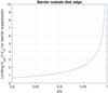 |
Fig. 11 Minimum value of Vout∕(−Vin) for full barrier suppression, as function of the ratio of the radii a∕b, for a circulardisk solar panel in vacuum, where Vout is positive. |
6 Simulation of concentric disks
To test and extend the validity of the analytical model in Sect. 5.1 to incorporate a plasma (and Debye shielding), we simulate two concentric disks at different bias potentials from the ground (0 and +75 V for the inner and outer disk, respectively) in SPIS. We take the models specified in Fig. 7 with a disc thickness of 5 mm and use the same environmentand materials as specified in Table 1 with a PIC treatment of all particles and simulate until the spacecraft potential converges. To improve statistics for the electrostatic potential in the volume, we utilise the symmetry of the problem in three dimensions (seen in Fig. 12). For plotting the potential along the z axis, we divided the axis into intervals of length dz. For each z value, we calculated the median value of the potential for all points between the planes defined by z and z+dz (as well as -z and -(z+dz)) which lie within ρ∕a = 0.2. For the plot of potential vs. ρ, we did the same for a ring-like volume containing all points between a cylinder of thickness dρ around ρ and within 2 degrees of the z = 0 plane.
Comparing the SPIS reference simulation to the vacuum case in Fig. 13, we find a potential barrier at the exact same position (as far as our SPIS simulations resolution allows) as our analytical model predicts. The absolute potential of the barrier UM is, unsurprisingly, smaller, as the plasma would screen all non-zero potentials via Debye shielding. The SPIS also allows us to run a series of simulations where we can change the Debye length of the plasma in the volume without changing the floating potential of the spacecraft (as changing the density or temperature of the plasma would undoubtedly shift the balance of currents to the spacecraft). These results are also shown in Fig. 13. The potential in the volume is more efficiently damped when moving away from the spacecraft as λD decreases and we can plot the fractional departure from the Sherman analytical model at the position of the barrier potential vs λD in each simulation in Fig. 14. Using the method of a least-squares fit to an appropriate model, we find that
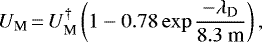 (10)
(10)
where UM is the SPIS barrier potential,  is the barrier potential in the vacuum solution, and λD is the Debye length. This model has the limit
  as expected for a vacuum. This particular model clearly does not describe the limit of very short Debye lengths correctly as UM here should go to zero, but it does well in describing the parameter range of our simulations and the transition to vacuum conditions.
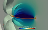 |
Fig. 12 3D visualisation of electrostatic potential structure for the SPIS concentric disks (a = 1.17 m, b = 1.25 m) simulation with VB = +75 V, coloured by electrostatic potential. To illustrate the potential in the volume, we plot the potential along the X–Z plane, as well as 10 equipotential surfaces from −30 V to +25 V, cut in the X-Y plane. The potential of the outer disk is −45.1 V and 29.9 V for the inner disk. |
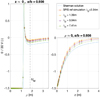 |
Fig. 13 Electrostatic potential normalised by potential of the positive outer ring (+30 V) along cylindrical axes, ρ (left) and z (right). For the vacuum case (blue line), the ring radii fraction, a, is identical to the SPIS model, and the absolute potential of the disks are taken from the output of the reference SPIS simulation (red circles). The associated analytical solution for the barrier potential, UM, is marked with a dashed black line. The other SPIS simulations were simulated at identical conditions except with fixed potentials on the rings, and with different plasma Debye lengths (modulated by changing the plasma density or electron temperaturein each simulation). |
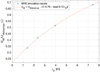 |
Fig. 14 Barrier potential for four SPIS PIC simulations at different Debye lengths with the same disk potentials, divided by the analytic vacuum model result (Sherman & Parker 1971). The fitted model is plotted in red. |
7 Spacecraft potential model
7.1 Model of current collection with barrier potential
At distances from a negatively charged object sufficiently large so that the potential has decayed by a few times, kB Te∕e, it follows fromLiouville’s theorem that the electron density equals the ambient plasma density reduced by a Boltzmann factor (Laframboise & Parker 1973).
As the potential is repelling from infinity up to the barrier, the plasma density at this point should be
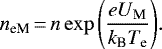 (11)
(11)
Olson et al. (2010) therefore proposed that the electron current, Iep, to a positive spherical probe within the negative barrier potential from a larger sphere some distance away is given by the standard orbital motion limited expression (Mott-Smith & Langmuir 1926) with the source density reduced by the Boltzmann factor at the barrier, viz.
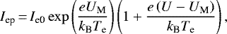 (12)
(12)
where  and it is further assumed that the current attraction is governed not by the absolute potential of the anode with respect to a plasma at infinity, but of the difference between the barrier potential and the anode. An electron passing the barrier may very well complete an orbit around the probe sphere and leave again, so the spherical probe form assumed by Olson et al. (2010) does not seem unrealistic. However, our case of an attracting ring on the edge of a repelling disk is quite different. An electron passing the barrier potential seen in Figs. 10a and b and Fig. 12 cannot encircle the anode along the disk edge in the poloidal direction and is efficiently focused toward the edge by the repelling field lines from the main solar panel. This is verified by our PIC simulations in which the current to the anode does not fit any spherical OML expression but is best described by the current collection to a plate of equal area. As such, Eq. (12) is simplified to
 (13)
(13)
7.2 Spacecraft potential from a current balance
Bringing it all together, we can estimate the electron current to positive biased elements in a plasma inside a barrier potential (if any) using Eqs. (5), (9), (10), and (13). Along with the expression for electron current to a negative surface in OML (Laframboise & Parker 1973), we find the general expression for the electron current to a charged solar panel within a barrier potential to be
 (14)
(14)
The ion current can be shown (Sagalyn et al. 1963) to be
 (15)
(15)
where Ei is the ion energy, and  . From the lessons learned in Sect. 4, we also reduce the photoemission on the spacecraft by a positive factor, γph ≤ 1, to simulate all interconnectors and bus bars scattered over the solar panels that reduce the net photoelectron production for the spacecraft. In this way, we can simplify the photoemission current expression in Grard (1973) for both surfaces to
 (16)
(16)
where dAU is the heliocentric distance in AU, and ra is the radius of the inner disk.
We find the equilibrium (spacecraft) potential for our solar panel when all currents to an inner disk at potential VS < UM and an outer disk at potential VS + VB, sum up to zero. After some rearranging to isolate VS from Eq. (14), we find
 (17)
(17)
where  is the sum of the currents
  and
and  as a function of potential (and barrier potential), and we use a superscript to separate terms for the inner and outer disks of radius a and b, respectively.
Now we have all the tools for predicting the current to the Rosetta solar panel without the need for computationally costly 3D PIC simulations. In an iterative solution of Eq. (17) of all currents to all surfaces on a concentric disk model of ten solar panels and a simple conductive and photo-emitting Rosetta SC box of 2 × 2 × 2.5 m, where we insert also a cold (0.1 eV) electron component that is otherwise computationally costly to simulate, we find the equilibrium spacecraft potential and the barrier potential. We plot the results in Fig. 15.
As we increase the cold electron component, we observe a significant negative charging up until a barrier potential is formed around VS ≈−27 V. Beyond this potential, or beyond the creation of a barrier potential, the electron density dependence on spacecraft potential tapers of rapidly as cold electrons can no longer reach the spacecraft (even when the net potential of the biased elements is still ≈ + 35 V). When comparing this result to Fig. 1, which prompted this study, we find an explanation for both the highly negative spacecraft potential and the strong dependence on cold electron density versus spacecraft potential below −25 V. As we move to larger heliocentric distances in Fig. 16, we shift the curve downwards as the photoemission current decreases everywhere and find a linear trend in the same regions of densities and potentials as in Fig. 1. In reality, the potential of the positive elements around the edge that we base our disk model upon should be distributed on some potential between +0.7 and +78 V and we see in Fig. 16 that for low bias potentials VB, the cold electron current has no coupling to the spacecraft or loses coupling even for low spacecraft charging as a potential barrier develops, indicating that moderate (absolute) positive potentials on the interconnects will have little effect on the Rosetta spacecraft current system.
In reality, Rosetta is not simply a set of solar panels and an ITO-coated spacecraft box but, rather, these represent the principle surfaces for photoemission and current collection and, as such, we believe that the current balance would only be slightly perturbed by incorporating a more realistic Rosetta spacecraft body. A more accurate shape model for the solar panels would increase the complexity of the barrier potential shape and the subsequent current collection to all surfaces, but it could be expected to have the same general behaviour in terms of the creation of barrier potentials and current collection to the positively biased surfaces. Introducing a flowing plasma and possible wakes associated with this flow may also alter the details of the balances, but wake effects should mostly be weak: those that are typically observed ion flow directions – between radially outward from the comet and anti-sunward (Berčič et al. 2018) – in combination with the Rosetta trajectory around 67P – with a mostly terminator orbit and its solar panel length axis along the direction perpendicular to the nucleus and the panels themselves normal to the sun – minimises wake effects on the solar panel front surface. We cannot be certain that all our simplifications are valid when moving to a more realistic model, but Figs. 1 and 16 show that we have found a candidate model that describes the general evolution of the spacecraft potential and current collection behaviour of cold electrons to Rosetta during its mission. Regardless of geometry, this current collection behaviour seen on Rosetta can only be represented by a positively biased conductor with sufficient bias to attract electrons beyond VS < −20 V and significant surface area to both overcome barrier potentials from surrounding surfaces as well as yield significant cold electron current. We also note that we do not see a decoupling of cold electrons to spacecraft potential in Fig. 1 even at the most negative potentials, which indicates that the positively biased surfaces are always (at least for this set of measurements taken between January to September 2016) large or positive enough that no negative barrier potential is formed. Therefore, as shown in Fig. 10, the solar array likely appears as net positive surfaces for a charged particle far away from the spacecraft.
On 12 July 2016, from 09:30 to 10:00 UTC, Rosetta conducted a solar array power test composed of a 60 deg rotation of the solar array from the sun, thus reducing the available solar power (and photoemission on the solar array) by 50 percent, along with, perhaps, a decrease of VB on the solar array anodes, as more strings would be at the maximum power point. At this moment, LAP registered a drop in spacecraft potential, from ≈−11.5 to ≈−17 V, plotted in Fig. 17, which is consistent with a spacecraft that is photo-emitting less. As the plasma parameters were otherwise relatively stable (no detected cold electron population, Tew ≈ 5 eV), this is a rare opportunity where we can compare these measurements to our model for various parameters in an attempt to constrain γph and possibly VB. In Fig. 17, we see that a decrease of 50 percent of photoemission, which in our model represents a 50 percent decrease in γph (from before the rotation) is compatible with our measurements for γph ≿ 0.4 in both absolute potential values and the relative potential drop, of which we suspect the latter to be a more relevant parameter, and γph = 0.8 gives us the best fit. What is also apparent in Fig. 17 is that we cannot put strong constraints on the positive bias VB, as there are nodetectable cold electrons.
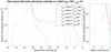 |
Fig. 15 Cold electron density vs. Spacecraft potential model solution (left) and barrier potential (right) for various cometary plasma parameters. |
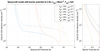 |
Fig. 16 Left: spacecraft potential model solution for a solar panel vs. nec at 2 AU, new = 80 cm−3, Tew = 4 eV at various bias potentials. Right: barrier potential in the model vs. nec. |
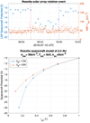 |
Fig. 17 Top: LAP spacecraft potential (blue circles) and MIP electron density (red dots) during a rotation of the Rosetta solar array of 60 deg from the sun, for which two dashed lines indicate the start (red) and end (blue) of the test. Bottom: spacecraft potential result at various γph and VB from an adaptation of our solar panel model to a Rosetta spacecraft box with ten panels, for which new = 50−3, Tew = 5 eV, at 3.4 AU with no cold electrons present. |
8 Conclusions
In our investigation of the correlation of the LAP measured Rosetta Spacecraft potential to the MIP measured densities and characteristic temperatures of two detected cometary electron populations, we find the spacecraft potential to depend more on electron density (particularly cold electron density) and much less on electron temperature than expected in the high flux of thermal (cometary) ionospheric electrons.
To investigate the current to the positively biased borders on the front-side panels of the Rosetta solar array, we first apply an analytical model to obtain the potential surrounding two concentric disks at different potentials in a vacuum. Comparing the result to 3D PIC SPIS simulations and constructing a simple model bridging the two, we arrive at a system of equations that can readily explain the strong relationship between the (highly negative) Rosetta spacecraft potential and an observed cold (0.1 eV) electron population that sometimes dominate the Rosetta electron environment even when barrier potential effects are considered. We find an explanation for the highly negative charging on the spacecraft, the seemingly poor coupling of electron temperature to spacecraft potential, and the observed log-lin relationship of electron density to spacecraft potential that is used in our analysis of LAP and MIP data to retrieve electron density estimates published on AMDA3 and soon on the ESA Planetary Science Archive.
To mitigate spacecraft charging on planetary plasma missions in the future, especially in dense, cold environments where low-energy plasma particles are of particular scientific importance, we suggest an inversion of polarities (i.e. setting spacecraft ground as the anode) in the solar array design, which would drastically reduce the current drawn from the plasma. This approach has been taken on ionospheric spacecraft like Atmospheric Explorer C and Swarm and been shown to result in a stable and slightly negative potential (Samir et al. 1979; Zuccaro & Holt 1982). Increased efforts to insulate positively biased conductors, where particular attention should be directed to areas close to edges of structures, would also help reduce spacecraft charging and enable more sensitive plasma measurements of the coldest plasma populations.
Acknowledgements
Rosetta is an ESA mission with contributions from its member states and NASA. This work would not have been possible without the collective efforts over a quarter of a century of all involved in the project and the RPC. We are also grateful to everybody who has worked on the SPIS software, at ONERA, ARTENUM and elsewhere, and to ESA for supporting this highly valuable package. This research was funded by the Swedish National Space Agency under grant Dnr 168/15. The cross-calibration of LAP and MIP data was supported by ESA as part of the Rosetta Extended Archive activities, under contract 4000118957/16/ES/JD.
References
- Bergman, S., Wieser, G. S., Wieser, M., Johansson, F. L., & Eriksson, A. 2019, J. Geophys. Res. Space Phys., 125, e2019JA027478 [Google Scholar]
- Bergman, S., Wieser, G. S., Wieser, M., Johansson, F. L., & Eriksson, A. 2020, J. Geophys. Res. Space Phys., 125, e2020JA027870 [Google Scholar]
- Berčič, L., Behar, E., Nilsson, H., et al. 2018, A&A, 613, A57 [NASA ADS] [CrossRef] [EDP Sciences] [Google Scholar]
- Berthelier, J.-J., & Roussel, J.-F. 2004, J. Geophys. Res., 109, A01105 [NASA ADS] [Google Scholar]
- Broiles, T. W., Burch, J. L., Chae, K., et al. 2016, MNRAS, 462, S312 [CrossRef] [Google Scholar]
- Carr, C., Cupido, E., Lee, C. G. Y., et al. 2007, Space Sci. Rev., 128, 629 [NASA ADS] [CrossRef] [Google Scholar]
- Carruth, M. R., J., Schneider, T., McCollum, M., et al. 2001, ESA SP, 476, 95 [NASA ADS] [Google Scholar]
- Edberg, N. J. T., Eriksson, A. I., Odelstad, E., et al. 2015, Geophys. Res. Lett., 42, 4263 [NASA ADS] [CrossRef] [Google Scholar]
- Engelhardt, I. A. D., Eriksson, A. I., Vigren, E., et al. 2018, A&A, 616, A51 [NASA ADS] [CrossRef] [EDP Sciences] [Google Scholar]
- Eriksson, A. I., & Wahlund, J.-E. 2006, IEEE Proc. Plasma Sci., 34, 2038 [NASA ADS] [CrossRef] [Google Scholar]
- Eriksson, A. I., Boström, R., Gill, R., et al. 2007, Space Sci. Rev., 128, 729 [NASA ADS] [CrossRef] [Google Scholar]
- Eriksson, A. I., Engelhardt, I. A. D., André, M., et al. 2017, A&A, 605, A15 [NASA ADS] [EDP Sciences] [Google Scholar]
- Garrett, H. B., Evans, R. W., Whittlesey, A. C., Katz, I., & Insoo Jun. 2008, IEEE Trans. Plasma Sci., 36, 2440 [CrossRef] [Google Scholar]
- Gilet, N., Henri, P., Wattieaux, G., et al. 2019, A&A, 640, A110 [Google Scholar]
- Grard, R. J. L. 1973, J. Geophys. Res., 78, 2885 [NASA ADS] [CrossRef] [Google Scholar]
- Henri, P., Vallières, X., Hajra, R., et al. 2017, MNRAS, 469, S372 [Google Scholar]
- Ivchenko, N., Facciolo, L., Lindqvist, P.-A., Kekkonen, P., & Holback, B. 2001, Ann. Geophys., 19, 655 [CrossRef] [Google Scholar]
- Johansson, F. L., Henri, P., Eriksson, A., et al. 2016, in Proceedings of the 14th Spacecraft Charging Technology Conference (European Space Agency) [Google Scholar]
- Laframboise, J. G., & Parker, L. W. 1973, Phys. Fluids, 16, 629 [NASA ADS] [CrossRef] [Google Scholar]
- Matéo-Vélez, J.-C., Sarrailh, P., Thiébault, B., et al. 2012, in Proceedings of the 12th Spacecraft Charging Technology Conference (SCTC-12) (JAXA) [Google Scholar]
- Mateo-Velez, J., Theillaumas, B., Sevoz, M., et al. 2015, IEEE Trans. Plasma Sci., 43, 2808 [CrossRef] [Google Scholar]
- Mott-Smith, H. M., & Langmuir, I. 1926, Phys. Rev., 28, 727 [CrossRef] [Google Scholar]
- Odelstad, E., Eriksson, A. I., Edberg, N. J. T., et al. 2015, Geophys. Res. Lett. 42, 10, 126 [Google Scholar]
- Odelstad, E., Stenberg-Wieser, G., Wieser, M., et al. 2017, MNRAS, 469, S568 [Google Scholar]
- Olson, J., Brenning, N., Wahlund, J., & Gunell, H. 2010, Rev. Sci. Instrum., 81, 105106 [NASA ADS] [CrossRef] [EDP Sciences] [Google Scholar]
- Roussel, J.-F., & Berthelier, J.-J. 2004, J. Geophys. Res., 109, A01104 [NASA ADS] [Google Scholar]
- Sagalyn, R. C., Smiddy, M., & Wisnia, J. 1963, J. Geophys. Res., 68, 199 [NASA ADS] [CrossRef] [Google Scholar]
- Samir, U., Gordon, R., Brace, L., & Theis, R. 1979, J. Geophys. Res., 84, 513 [NASA ADS] [CrossRef] [Google Scholar]
- Sarrailh, P., Matéo-Vélez, J.-C., Hess, S. L., et al. 2015, IEEE Trans. Plasma Sci., 43, 2789 [CrossRef] [Google Scholar]
- Sherman, C., & Parker, L. W. 1971, J. Appl. Phys., 42, 870 [NASA ADS] [CrossRef] [Google Scholar]
- Stenberg Wieser, G., Odelstad, E., Wieser, M., et al. 2017, MNRAS, 469, S522 [NASA ADS] [CrossRef] [Google Scholar]
- Trotignon, J.-G., Michau, J. L., Lagoutte, D., et al. 2007, Space Sci. Rev., 128, 713 [NASA ADS] [CrossRef] [Google Scholar]
- Wattieaux, G., Gilet, N., Henri, P., Vallières, X., & Bucciantini, L. 2019, A&A, 630, A41 [NASA ADS] [CrossRef] [EDP Sciences] [Google Scholar]
- Wattieaux, G., Henri, P., Gilet, N., Vallieres, X., & Deca, J. 2020, A&A, 638, A124 [NASA ADS] [CrossRef] [EDP Sciences] [Google Scholar]
- Zuccaro, D. R., & Holt, B. J. 1982, J. Geophys. Res., 87, 8327 [NASA ADS] [CrossRef] [Google Scholar]
The string voltage on the solar array is driven by many parameters, including the temperature and degradation of the cells and the power requested by the spacecraft.
All Tables
All Figures
|
Fig. 1 2D histogram in 80 × 100 bins of 88 000 events of simultaneously measured spacecraft potential versus electron density (left column) and temperature (right column) from January to September 2016 at 2 to 3.8 AU. The identified electron populations by MIP from Wattieaux et al. (2020) are separated by temperature as warm (Tew ≈ 4 eV, top row) andcold (Tec ≈ 0.1 eV, bottom row).In total, 9700 outliers with either Tew > 15 eV (9400 outliers) or Tec > 0.5 eV (2800 outliers) have been removed. |
| In the text | |
|
Fig. 2 Top: example time series of LAP spacecraft potential (diamonds), cold (circles), and warm (pluses) electron density estimates from MIP in the same interval, exhibiting the strong correlation between spacecraft potential and cold electron density. Middle: same data as shown in Fig. 1, 2D histogram of 120 × 150 bins of new vs. eVS ∕Tew. Bottom: as above, but with nec on the y-axis. |
| In the text | |
|
Fig. 3 Rosetta spacecraft and one of its solar wings. The solar cell cover glass on each cell is visible as small dark glossy surfaces, with metallic reflective interconnects above and below it. There are also 25 slightly larger reflective bus bar pairs, not to be confused with the six circular Kevlar cutter/hold-down points. Adapted from Rosetta Solar panels on ESA’s website. Retrieved May 4, 2020, from sci.esa.int/s/w0e6nbW. Copyright 2012 ESA-A, Van der Geest. Reprinted with permission. |
| In the text | |
|
Fig. 4 Artistimpression of a corner section of the front side of a solar panel on Rosetta. The black squares are individual solar cells covered with grounded cover glass, connected in series via (pink) interconnects in a column that wrap around to the next column near the top edge (and bottom, not shown) of the solar panel via a longer interconnect (also pink). At the start and end of each string of 91 solar cells are bus bars, marked with red (anode) and blue (cathode). The grey circle represents one of six circular Kevlar cutter/hold-down points. All surfaces coloured in pink and red are exposed positively biased conductors. |
| In the text | |
|
Fig. 5 Visualisation of electrostatic potential struture from a SPIS simulation of a model with four 0.1 × 0.1 m +75V biasedelements on a 1.25 × 1.25 × 0.15 m solar panel inside a spherical simulation volume of radius 15 m. Ten equipotential surfaces (cut in the Y = Z plane) from −17 V to +42.5 V are also plotted with the −8 V and −17 V surfaces specifically labelled. |
| In the text | |
|
Fig. 6 Top: spacecraft (ground) potential evolution in five SPIS simulations. The reference simulation with no biased surfaces in a warm Tew = 10 eV plasma (blue line), with small charged surfaces of +75 V in a PIC simulation (black) or a fluid Maxwell-boltzmann simulation (yellow dot-dashed line). Also plotted, a simulation of the same plasma density but with 50 percent Tec = 0.1 eV electrons with either no biased surfaces (red), or with biased surfaces using the fluid approximation (purple dot-dash line). The Maxwell-Boltzmann simulations with surfaces at +75 V are strictly not valid but serve to illustrate the first approximation from Orbital-Motion-Limited theory. Bottom: zoom-in of above, with the calculated mean (dashed black line) and a 1σ range (dotted black lines) of spacecraft potential from the PIC simulation in this interval. |
| In the text | |
|
Fig. 7 Geometry of the concentric disk model for modelling of solar panels with biased elements as described in Sect. 5.1 for two different applications. Panel a: single exposed biased conductor on the main area of the solar panel (Sect. 5.2); panel b: exposes biased conductors along the edge (Sect. 5.3). Grey areas represent the main solar panel at spacecraft potential, red a biased element. |
| In the text | |
|
Fig. 8 Limiting potential ratio for barrier suppression for a small biased element on the z axis as given by Eq. (7). |
| In the text | |
|
Fig. 9 Vacuum potential and electric field pattern in the ρ−z plane near the centre of a thin circular disk of radius b as sketched in Fig. 7a. The disk potential outside ρ = a is Vin = −10 V while the potential Vout in the centre ρ < a varies as stated above each panel. In all cases, a = 0.02 b. Numerically integrated electric field lines are plotted in white. The 0 V equipotential is shown in thick red; the potential is zero also at infinity. Black curves indicate equipotentials at every integer value (in volts), with the background colour further highlighting the potential. |
| In the text | |
|
Fig. 10 Vacuum potential and electric field pattern in the ρ−z plane around a thin circular disk of radius b as sketched in Fig. 7b. The disk potential inside ρ = a is Vin = −10 V while the potential Vout in the annulus a < ρ ≤ b varies as stated above each panel. In all cases, a = 0.98 b. Numerically integrated electric field lines are plotted in white. The 0 V equipotential is shown in thick red; the potential is zero also at infinity. Black curves indicate equipotentials at every integer value (in volts), with the background colour further highlighting the potential. The magenta star indicates the location of minimum electron barrier height. |
| In the text | |
|
Fig. 11 Minimum value of Vout∕(−Vin) for full barrier suppression, as function of the ratio of the radii a∕b, for a circulardisk solar panel in vacuum, where Vout is positive. |
| In the text | |
|
Fig. 12 3D visualisation of electrostatic potential structure for the SPIS concentric disks (a = 1.17 m, b = 1.25 m) simulation with VB = +75 V, coloured by electrostatic potential. To illustrate the potential in the volume, we plot the potential along the X–Z plane, as well as 10 equipotential surfaces from −30 V to +25 V, cut in the X-Y plane. The potential of the outer disk is −45.1 V and 29.9 V for the inner disk. |
| In the text | |
|
Fig. 13 Electrostatic potential normalised by potential of the positive outer ring (+30 V) along cylindrical axes, ρ (left) and z (right). For the vacuum case (blue line), the ring radii fraction, a, is identical to the SPIS model, and the absolute potential of the disks are taken from the output of the reference SPIS simulation (red circles). The associated analytical solution for the barrier potential, UM, is marked with a dashed black line. The other SPIS simulations were simulated at identical conditions except with fixed potentials on the rings, and with different plasma Debye lengths (modulated by changing the plasma density or electron temperaturein each simulation). |
| In the text | |
|
Fig. 14 Barrier potential for four SPIS PIC simulations at different Debye lengths with the same disk potentials, divided by the analytic vacuum model result (Sherman & Parker 1971). The fitted model is plotted in red. |
| In the text | |
|
Fig. 15 Cold electron density vs. Spacecraft potential model solution (left) and barrier potential (right) for various cometary plasma parameters. |
| In the text | |
|
Fig. 16 Left: spacecraft potential model solution for a solar panel vs. nec at 2 AU, new = 80 cm−3, Tew = 4 eV at various bias potentials. Right: barrier potential in the model vs. nec. |
| In the text | |
|
Fig. 17 Top: LAP spacecraft potential (blue circles) and MIP electron density (red dots) during a rotation of the Rosetta solar array of 60 deg from the sun, for which two dashed lines indicate the start (red) and end (blue) of the test. Bottom: spacecraft potential result at various γph and VB from an adaptation of our solar panel model to a Rosetta spacecraft box with ten panels, for which new = 50−3, Tew = 5 eV, at 3.4 AU with no cold electrons present. |
| In the text | |
Current usage metrics show cumulative count of Article Views (full-text article views including HTML views, PDF and ePub downloads, according to the available data) and Abstracts Views on Vision4Press platform.
Data correspond to usage on the plateform after 2015. The current usage metrics is available 48-96 hours after online publication and is updated daily on week days.
Initial download of the metrics may take a while.