| Issue |
A&A
Volume 640, August 2020
|
|
|---|---|---|
| Article Number | A110 | |
| Number of page(s) | 20 | |
| Section | Planets and planetary systems | |
| DOI | https://doi.org/10.1051/0004-6361/201937056 | |
| Published online | 21 August 2020 | |
Observations of a mix of cold and warm electrons by RPC-MIP at 67P/Churyumov-Gerasimenko
1
Laboratoire de Physique et Chimie de l’Environnement et de l’Espace (LPC2E), CNRS, Université d’Orléans, Orléans,
France
e-mail: This email address is being protected from spambots. You need JavaScript enabled to view it.
2
Laboratoire Lagrange, OCA, UCA, CNRS,
Nice,
France
3
Université de Toulouse, LAPLACE-UMR 5213,
31062
Toulouse,
France
4
Swedish Institute of Space Physics,
Box 537,
75121
Uppsala,
Sweden
5
Department of Physics and Astronomy, Uppsala University,
Box 516,
75210
Uppsala,
Sweden
6
Physikalisches Institut, University of Bern,
Sidelerstrasse 5,
3012
Bern,
Switzerland
Received:
5
November
2019
Accepted:
17
June
2020
Abstract
Context. The Mutual Impedance Probe (MIP) of the Rosetta Plasma Consortium (RPC) onboard the Rosetta orbiter which was in operation for more than two years, between August 2014 and September 2016 to monitor the electron density in the cometary ionosphere of 67P/Churyumov-Gerasimenko. Based on the resonance principle of the plasma eigenmodes, recent models of the mutual impedance experiment have shown that in a two-electron temperature plasma, such an instrument is able to separate the two isotropic electron populations and retrieve their properties.
Aims. The goal of this paper is to identify and characterize regions of the cometary ionized environment filled with a mix of cold and warm electron populations, which was observed by Rosetta during the cometary operation phase.
Methods. To reach this goal, this study identifies and investigates the in situ mutual impedance spectra dataset of the RPC-MIP instrument that contains the characteristics of a mix of cold and warm electrons, with a special focus on instrumental signatures typical of large cold-to-total electron density ratio (from 60 to 90%), that is, regions strongly dominated by the cold electron component.
Results. We show from the observational signatures that the mix of cold and warm cometary electrons strongly depends on the cometary latitude. Indeed, in the southern hemisphere of 67P, where the neutral outgassing activity was higher than in northern hemisphere during post-perihelion, the cold electrons were more abundant, confirming the role of electron-neutral collisions in the cooling of cometary electrons. We also show that the cold electrons are mainly observed outside the nominal electron-neutral collision-dominated region (exobase), where electrons are expected to have cooled down. This which indicates that the cold electrons have been transported outward. Finally, RPC-MIP detected cold electrons far from the perihelion, where the neutral outgassing activity is lower, in regions where no electron exobase was expected to have formed. This suggests that the cometary neutrals provide a more frequent or efficient cooling of the electrons than expected for a radially expanding ionosphere.
Key words: comets: individual: 67P/Churyumov-Gerasimenko / instrumentation: detectors / elementary particles / methods: observational
© N. Gilet et al. 2020
 Open Access article, published by EDP Sciences, under the terms of the Creative Commons Attribution License (http://creativecommons.org/licenses/by/4.0), which permits unrestricted use, distribution, and reproduction in any medium, provided the original work is properly cited.
1 Introduction
As a comet nucleus approaches the Sun, the solar thermal forcing increases and the cometary volatiles sublimate so that the outgassing activity of neutral particles increases (e.g., Hansen et al. 2016). A cometary atmosphere, mainly composed of water, carbon monoxide and carbon dioxide (Gasc et al. 2017; Hoang et al. 2017), expands because of the low cometary gravity. This atmosphere gets ionized through different mechanisms (Cravens et al. 1987; Galand et al. 2016; Héritier et al. 2017, 2018): (i) by photoionisation by extreme ultra violet solar flux, (ii) by electron-impact ionisation by energetic electrons or, (iii) by solar wind impact ionisation and charge exchange, to form a cometary ionosphere that eventually interacts with the surrounding solar wind plasma. The plasma surrounding the comet nucleus is characterized by the coexistence of several electron populations. First, the electrons released by photoionisation are expected to have a temperature, Te, around 10 eV (Vigren & Galand 2013). Second, electrons at lower temperatures, resulting from the cooling by neutral-plasma interactions, can be observed (Engelhardt et al. 2018). The cometary neutrals are expected to have a temperature around 0.01 eV (Gulkis et al. 2015). Therefore, the temperature of the electrons cooled by the neutrals can decrease down to the temperature of the neutrals themselves. Third, as the comet evolves in the solar system, high-energy electrons (>20 eV) of solar wind origin can be observed around the nucleus (Myllys et al. 2019).
Previous cometary space missions confirmed the presence of several electron populations in the ionised environment of a comet. For instance, two plasma experiments on board the International Cometary Explorer (ICE) spacecraft characterized the electrons in the tail of the comet 21P/Giacobini-Zinner (von Rosenvinge et al. 1986). The electron spectrometer measured a hot component (~80 eV) considered as the halo component of the solar wind plasma, a mixed component (~10 eV) and a third component (~4 eV) resulting from photoionisation of the coma gas (Zwickl et al. 1986). At the same time, the thermal plasma noise spectroscopy experiment measured a decrease of the electron temperature from a warm component (~12 eV) to a slightly colder component (~1 eV) when the ICE spacecraft came closer to the nucleus (Meyer-Vernet et al. 1986). These two observationsof the electrons were only possible during one fly-by at large distances from the nucleus (~7800 km). Therefore, the origin and the evolution of the different electron populations during a comet life cycle were out of scope.
More recently, the Rosetta spacecraft escorted the comet 67P/Churyumov-Gerasimenko (Churyumov & Gerasimenko 1972) (hereafter 67P) during more than two years, from August 2014 to September 2016. Three instruments from the Rosetta Plasma Consortium (RPC, Carr et al. 2007) monitored the plasma properties such as the electron density and the electron temperature in different electron energy ranges: the Ion-Electron Sensor (RPC-IES, Burch et al. 2007), the Langmuir Probes (RPC-LAP, Eriksson et al. 2007) and the Mutual Impedance Probe (RPC-MIP, Trotignon et al. 2007). RPC-LAP and RPC-IES have already characterized different electron populations around 67P. Through the 3D-electron velocity distribution functions (EVDF) measured by the particle spectrometer RPC-IES, the density and the temperatureof the warm and the hot electron populations have been extracted by a fitting method between the in situ observed evdf and a dataset of synthetic EVDF modeled by a double-Kappa functions (Clark et al. 2015; Broiles et al. 2016a,b; Myllys et al. 2019). At the beginning of the cometary phase of the Rosetta mission far from the perihelion (~3 AU), Broiles et al. (2016b) found a hot component (~0.01 cm−3 and ~40 eV) seen as suprathermal electrons with a solar wind origin and a dense warm component (~10 cm−3 and ~16 eV). Recently, Myllys et al. (2019) extended the fitting method to all heliocentric distances. They showed that the warm population temperature remained roughly constant (~5–10 eV) while the hot population became hotter (from ~15 to ~25 eV) when the comet was close to perihelion.
The warm electron population was monitored by RPC-LAP and RPC-MIP. The temperature of the warm population was characterized by RPC-LAP around 3–10 eV through the measurement of the spacecraft potential (Odelstad et al. 2015) while RPC-MIP monitored this electron core density through the measurement of the electron plasma frequency (Chasseriaux et al. 1972). Furthermore, these two instruments measured, with independent methods, a cold electron component (~0.1 eV) that appears to be mixed with the warm electron component (Gilet et al. 2017; Engelhardt et al. 2018; Odelstad et al. 2018; Wattieaux et al. 2019). The cold electrons have a strong effect on the classical measurement of the current-voltage characteristic from the Langmuir probes (Eriksson et al. 2017) and the presence of cold electrons can be detected by RPC-LAP when these cold electrons dominate the plasma.
From the RPC-MIP point of view, the mutual impedance spectrum analysis is assisted by the theory and the modeling of the instrument response. Indeed, the instrument response strongly depends on both the electron velocity distribution function and the spacecraft geometry. The effect of simplified EVDF on the probe response has been studied in several theoretical papers during the past decades (Grard 1969; Navet et al. 1971; Chasseriaux et al. 1972; Béghin 1995). Recently, Gilet et al. (2017) modeled the instrument response for an idealized mutual impedance probe in a plasma modeled by two isotropic Maxwellian EVDF (named two-electron temperature plasma in the following), using interplanetary plasma conditions where the Debye length is of the order of the transmitter-receiver distance. This study showed that in certain plasma conditions, two clear resonances are visible on the synthetic mutual impedance spectra in presence of a mix of two electron populations characterized by different temperatures. Furthermore, Wattieaux et al. (2019) applied the modeling of the electrostatic potential to the mutual impedance response for the RPC-MIP instrument by taking into account the instrument and spacecraft geometry and, more important, spacecraft charging. Indeed, Rosetta was often observed to be at a negative floating potential (Odelstad et al. 2017), so that the electrons are repelled by the spacecraft and the boom where RPC-MIP is located. Such conditions are responsible for the formation of an (electron depleted) ion sheath surrounding the RPC-MIP instrument, where the electrons are not present. To take into account this important property, Wattieaux et al. (2019) modeled the instrument response using the discrete-surface-charge-distribution (DSCD) method (Béghin & Kolesnikova 1998; Geiswiller et al. 2001) that consists in considering each charging surface on the spacecraft as a transmitter, and for the first time, also considering a plasma sheath surrounding the instrument. They showed that in a two-electron temperature plasma, a double resonance can be visible on the synthetic RPC-MIP spectra for a large enough cold-to-total density ratio (from 60 to 90%) and a large enough warm-to-cold temperature ratio (>20). In this study, we focus on this regime, which is characterized by a large fraction of cold cometary electrons.
During the cometary phase of the Rosetta mission, RPC-MIP measured a variety of mutual impedance spectra exhibiting such features and indicating the presence of a mixture of cold and warm electron populations in the ionosphere of 67P. During this time period,the Rosetta spacecraft orbited around the comet 67P at all latitudes and at all longitudes. The cometocentric distance of Rosetta varied from few kilometers (down to the surface of 67P after landing at the end of the mission) to 1500 km after two excursions (Taylor et al. 2017). The heliocentric distance varied from 3.6 AU at the beginning of the mission, to 1.25 AU at the perihelion, and back to 3.8 AU at the end of the cometary operations. Therefore, the RPC-MIP instrument measured mutual impedance spectra (i) in a large range of different locations around the comet and (ii) in a large heliocentric distance range from the Sun. The goal of this paper is to make use of this large dataset to (i) give an overview of the cold electrons observed by the mutual impedance probe RPC-MIP during the cometary phase mission using the double resonance observations on the mutual impedance spectra and (ii) discuss the origin of those cold cometary electrons.
The paper is organized as follows. First, RPC-MIP and RPC-LAP instruments and the acquired dataset are described in Sect. 2. Second, we detail the features observed on the RPC-MIP spectra in presence of a two-electron temperatureplasma through the modeling of the instrument response in Sect. 3. We show that the spectral signature of interest, namely a double resonance in the mutual impedance spectra, can only be observed in certain operational modes of RPC-MIP. The modeling of RPC-MIP spectra is used to explain this property and select the operational mode that is most favorable to the study of cold cometary electrons. We also provide an overview of the observation of cold electrons by RPC-MIP for the whole cometary phase of the Rosetta mission. Third, in Sect. 4, we study the observations of cold electrons by RPC-MIP with the parameters of interest (latitude, longitude, cometocentric distance, …). We show that the cold electron detections are observed at all heliocentric distances (near perihelion at 1.25 AU to the end of the mission at 3.8 AU), but preferentially in the hemisphere characterized by a higher outgassing activity. Furthermore, cold electrons were even observed when the electron-neutral collision-dominated region (Mandt et al. 2016) – where electrons are expected to have cooled down – was not expected to have formed. Finally, in Sect. 5, we compare theobservation of cold electrons of RPC-MIP with the detections made by RPC-LAP. We also discuss the origin of thecold electrons observed by the two instruments. We present our conclusions in Sect. 6.
2 Instrumentation and data
In this section, we describe the two plasma instruments onboard Rosetta that will be considered in this study: the Mutual Impedance Probe (RPC-MIP, Sect. 2.1) and the Langmuir Probes (RPC-LAP, Sect. 2.3). We also describe the RPC-MIP dataset composed of the in situ acquired mutual impedance spectra and we present the method to determine the thermal electron density from the mutual impedance spectra (Sect. 2.2).
2.1 RPC-MIP experiment
The Mutual Impedance Probe (RPC-MIP) onboard the Rosetta orbiter monitored the plasma bulk properties of the ionosphere of 67P/Churyumov-Gerasimenko (Trotignon et al. 2007). As a part of the RPC (Carr et al. 2007), the type of experiment was designed to assess the thermal electron density and, under certain plasma conditions, the electron temperature of the surrounding plasma (Chasseriaux et al. 1972). The mutual impedance probe is based on the resonance principle of the propagation of plasma eigenmodes (Krall & Trivelpiece 1973) in order to extract the characteristic frequencies of the surrounding plasma, in particular the electron plasma frequency, directly related to the electron density.
Since the beginning of space exploration, this kind of experiment was deployed in several space missions onboard spacecraft or rockets in planetary environments such as the Earth ionosphere or magnetosphere (Storey et al. 1969; Béghin & Debrie 1972; Décréau et al. 1978; Béghin et al. 1982) and for the first time with RPC-MIP, in the interplanetary plasma. Moreover, the Active Measurement of Mercury’s Plasma (AM2P) experiment (Trotignon et al. 2006) from the Plasma Wave Investigation (PWI) (Kasaba et al. 2020) as part of the payload of the BepiColombo Mio/MMO spacecraft (JAXA) will characterize the Hermean magnetospheric and the near-Mercury solar wind plasma. Furthermore, a similar experiment will be also deployed for the JUICE (Jupiter ICy Moons Explorer) mission. This mutual impedance experiment, called Mutual Impedance Measurement (MIME), part of the Radio Wave Plasma Investigation (RPWI), will monitor the plasma bulk properties on the Jovian system and in particular the ionosphere of Ganymede. Finally, a mutual impedance experiment is currently planned for the future mission Comet Interceptor (Snodgrass & Jones 2019). This mission will characterize a dynamicallynew comet with multi-point measurements made by a main spacecraft and two accompanying daughter spacecrafts.
The RPC-MIP experiment (Trotignon et al. 2007) is an active instrument composed of two receiving and two transmitting electrodes, carried by a 1m-long bar, mounted at the edge of a 1.8-m boom (Fig. 1). The transmitters (E1 and E2) inject a frequency-dependent current I(ω) while the receivers (R1 and R2) measure the difference of (complex) amplitude of the electric potential  at the same frequency ω. The complex impedance Z(ω) = V (ω)∕I(ω) derived from the coupling between the transmitters and the receivers depends on the plasma properties. By onboard Fourier analysis of the instrument temporal response, a mutual impedance spectrum can be built by varying, step by step, the emitted frequency around the expected characteristic frequencies of the encountered medium. The frequency range of the RPC-MIP goes from 32 kHz to 1 MHz.
To isolate the effect of the plasma on the potential radiated by the emission part of a mutual impedance probe, we work with the mutual impedance spectrum normalized to the spectrum that is obtained in vacuum
 (1)
(1)
where ΔZ and ΔZ0 represent the mutual impedance of a probe surrounded by a plasma and in vacuum, respectively, and  (resp.
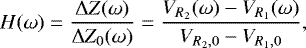
  ) is the voltage measured by the receiver Ri in the plasma (resp. in vacuum). A typical mutual impedance spectrum acquired by RPC-MIP is shown in Fig. 2.
During the cometary phase of the Rosetta mission, RPC-MIP operated in two main modes. The first mode, named Short Debye Length (SDL), has been designed for a surrounding cometary plasma where the typical Debye length is of the order of – or shorter than – the transmitter-receiver distance that is, λD < 40 cm.
Density measurements can be extended to lower densities that is, larger Debye lengths, up to about 2 m - by using the so-called Long Debye Length (LDL) mode. In this mode, the LAP2 spherical probe (Fig. 1) is used as a transmitter, located at about 4 m from the RPC-MIP receivers, while the RPC-MIP transmitters E1 and E2 are switched off. However, the LDL mode operated in an emission frequency range that does not exceed 168 kHz which is not sensitive to plasma densities above about 350 cm−3. Since cold electrons were observed where the total electron density was usually higher than this value, this study only focuses on measurements done with the SDL mode. The SDL mode can be used with four different SDL operational sub-modes called E1, E2, anti-phased and phased. In the E1 (resp. E2) sub-mode, only the transmitter E1 (resp. E2) transmits actively a potential in the plasma, which is measured by the two receivers R1 and R2. In anti-phased (resp. phased) SDL sub-mode, the two transmitters actively emit a potential in the plasma, both in phase opposition (resp. in phase). The use of the four SDL sub-modes during the whole mission is discussed in Sect. 3.3. Each of these SDL operational sub-modes has been used at different time rates and the cadence of the RPC-MIP measurements might vary during the comet phase: from a lower time resolution in the so-called “normal mode” (~32 s in SDL mode) to a higher-cadence measurement in the so-called “burst mode” (~3.5 s in SDL mode).
 |
Fig. 1 (a) Mutual Impedance Probe (RPC-MIP) onboard the Rosetta spacecraft consists of two transmitters (E1 and E2) and two receivers (R1 and R2) carried by a 1m-long bar (picture adapted from Trotignon et al. (2006)) and (b) RPC-MIP location at the edge of a 1.8-m boom on the Rosetta spacecraft and location of the two Langmuir probes RPC-LAP1 and RPC-LAP2 (Copyright: ESA/ATG medialab). |
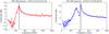 |
Fig. 2 Two typical in situ acquired RPC-MIP mutual impedance spectra (after compensation of instrumental effects such as interferences and solar wind response removal) in the ionosphere of 67P, from which the electron plasma frequency, fp, (shown by a vertical black line) is obtained, both in a plasma dominated by a warm electron population and characterized by a single resonance (left panel), and in a plasma characterized by a mixture of warm and cold electron populations and characterized by a double resonance (right panel). For the first (resp. second) spectrum, fp = 274 kHz (resp. fp = 421 kHz) corresponding to ne = 924 cm−3 (resp. ne = 2198 cm−3). These two spectra have been measured with the RPC-MIP phased SDL sub-mode. |
2.2 RPC-MIP dataset
The main dataset of the RPC-MIP experiment consists of mutual impedance spectrograms (Henri et al. 2017; Hajra et al. 2018). Plasma bulk properties can be extracted from the shape of the mutual impedance spectrum such as the electron density if: (i) the electron plasma frequency is contained in the operated frequency range and (ii) the Debye length is lower than the transmitter-receiver distance (Chasseriaux et al. 1972). This experiment measures the plasma waves, depending on the surrounding plasma and the magnetic field properties. For instance, during the three Rosetta Earth fly-bys, RPC-MIP measured the electron cyclotron frequency and its harmonics, together with the electron plasma frequency in the Earth magnetosphere (Béghin et al. 2017). However, in the cometary plasma the ambient magnetic field amplitude is too weak for a detection of the electron cyclotron frequency by RPC-MIP and only the electron plasma frequency can be detected.
The electron plasma frequency, fp, is extracted in the close vicinity of the principal resonance in the mutual impedance spectra. Note that the electron plasma frequency can be shifted from the frequency corresponding to the maximum amplitude, in particular in the case where the electron density is low that is, the Debye length is of the order of the transmitter-receiver distance. The total electron density, ne, is then directly determined from the identification of the electron plasma frequency on the mutual impedance spectra.
A typical in situ acquired RPC-MIP mutual impedance spectrum where the instrument operated in phased SDL sub-mode in the cometary plasma is shown in Fig. 2 (left panel). Note that all of the RPC-MIP spectra shown in this study have been cleaned up of instrumental artifacts, such as two known interferences around 150 and 250 kHz, deleted by a linear interpolation. For each mode, the amplitude of the mutual impedance response in vacuum is computed by a mean of a large number of acquired spectra where the spectrum is flat, typically obtained when the electron density is too low for any detection that is, in the solar wind plasma. All spectra have been normalized by the mutual impedance response in the solar wind (solar wind response hereafter). For the spectrum shown in Fig. 2 (left panel), acquired in the cometary plasma, the plasma frequency, fp, is identified as the maximum (vertical black line), with fp = 273 kHz, corresponding to a total electron density ne = 924 cm−3.
2.3 RPC-LAP experiment
RPC-LAP consists of two spherical Langmuir probes (LAP1 and LAP2, see Fig. 1) that are able to monitor different plasma parameters such as the electron density, the electron temperature or the spacecraft potential (Eriksson et al. 2007; Odelstad et al. 2015). In this study, we focus on the classical measurement made by a Langmuir probe: the current-voltage (I-V) curve that corresponds to a sweep through voltages while the probe measures the resulting current. A typical I-V curve can be found in Eriksson et al. (2017, Fig. 2).
The RPC-LAP usually measured a current-voltage curve every 160 s in normal mode and every 64 s in LDL mode. These measurements enable to constrain the value of the electron density ne and the electron temperature Te, and are therefore highly complementary to the RPC-MIP measurements. RPC-LAP was able to detect a cold electron population during a significant part of the cometary operation of the Rosetta orbiter around comet 67P (Eriksson et al. 2017; Engelhardt et al. 2018). We discuss the comparison between the observations of cold electrons made by RPC-MIP and RPC-LAP in Sect. 5.
3 Detection capabilities of cold cometary electrons by RPC-MIP
In this section, we provide a study of the RPC-MIP capabilities for the detection of the cold cometary electrons. First, we characterize the cold electron signature in RPC-MIP spectra and show its dependence on the plasma conditions in Sect. 3.1. Second, we provide an overview of the cold cometary electron detections during the whole cometary phase of theRosetta mission (Sect. 3.2). Finally, we investigate the dependence of the detection of the cold electrons on the operational SDL sub-mode (Sect. 3.3).
3.1 Cold cometary electron identification on synthetic mutual impedance spectra
The effect of a mixture of two electron populations on the measurement of the mutual impedance spectra has been characterized by Gilet et al. (2017) for an idealized mutual impedance probe and by Wattieaux et al. (2019) for the RPC-MIP experiment by taking into account the instrument and the spacecraft charging. By numerical modeling of the electrostatic potential induced by a transmitting electrode in the surrounding plasma, they computed synthetic mutual impedance spectra in a two-electron temperature plasma modeled by a sum of two Maxwellian EVDF. Both studies found that in some plasma conditions, depending on the electron density and temperature between the two populations, the amplitude of the mutual impedance spectrum exhibits a characteristic double resonance. This feature can be explained by the fact that the mutual impedance experiment is based on the resonance principle of plasma eigenmodes (Krall & Trivelpiece 1973; Storey 1998). Indeed, these plasma eigenmodes determine the resonances that shape the mutual impedance spectra (see Sect. 2.2). In a plasma modeled by a single or a double-Maxwellian EVDF, there exists an infinite number of eigenmodes (Derfler & Simonen 1969; Chasseriaux et al. 1972; Gary 1993; Béghin 1995; Gilet et al. 2017). However, only the least damped poles have a strong effect on the propagation of the electrostatic potential radiated by the transmitter of the mutual impedance probe (Chasseriaux et al. 1972; Gilet et al. 2017).
In a Maxwellian plasma, the least damped poles are the Langmuir modes. The corresponding waves propagate at frequencies higher than the total electron plasma frequency fp. In an unmagnetized plasma, the Langmuir waves are responsible of the resonance located in the mutual impedance spectra close to fp which enable to retrieve the total electron density of the surrounded plasma.
In a plasma characterized by a sum of two Maxwellian EVDF, two main eigenmodes propagate in the surrounded plasma: (i) the modified Langmuir waves, propagating for frequencies higher than fp, and (ii) the electron acoustic modes, propagating for frequencies smaller than fp (Gary 1993; Gilet et al. 2017). The superposition of these two waves produces a double resonance in the mutual impedance spectra, the main one located close to the total electron plasma frequency, fp, and another one at a lower frequency, close to the plasma frequency of the colder electron population. Gilet et al. (2017) modeled the mutual impedance response in an idealized case, where the mutual impedance probe is totally immersed in the plasma and where the transmitters are seen as single pulsating point charges. However, this modeling of the mutual impedance spectra does not take into account two strong effects that can affect the in situ observations: (i) the conducting Rosetta orbiter and structure of the RPC-MIP probe, and (ii) the plasma sheath surrounding the orbiter and the instrument because of spacecraft charging. The influence of the plasma sheath on the mutual impedance response has been studied by Wattieaux et al. (2019) using a discrete-surface-charge-distribution (DSCD) method (Béghin & Kolesnikova 1998; Geiswiller et al. 2001). Wattieaux et al. (2019) has shown that, in the case of the RPC-MIP instrument configuration used in the so-called SDL mode, and with the typical parameters encountered in the cometary plasma by Rosetta, the characteristic double resonance is visible on mutual impedance spectra for a cold-to-total density ratio larger than 60% and a warm-to-cold temperature ratio higher than 30. Several examples of synthetic mutual impedance spectra are given in Appendix B.2, using different models of the RPC-MIP instrument response each showing the appearance of an extra, second, resonance below the plasma frequency in this parameter regime, confirming the robustness of this spectral signature.
In this study, we make direct use of this robust spectral signature to detect the presence of a mix of cold and warm electrons around comet 67P, in regions dominated by the cold electron population (from 60 to 90%). An ad-hoc algorithm has been developed in order to detect the double resonances in the entire RPC-MIP dataset. This algorithm is detailed in Appendix C. An example of a typical in situ acquired RPC-MIP spectrum showing such double resonance is shown in Fig. 2 (right panel). The total electron plasma frequency is located at 421 kHz corresponding to a total electron density equals to 2200 cm−3. In the following section, we study the dataset of the RPC-MIP spectra acquired during the whole cometary phase of the mission in order to characterize the RPC-MIP capabilities for detection of the cold electrons in the ionosphere of 67P.
3.2 Overview of the detection and the location of cold cometary electrons observed in situ by RPC-MIP
An overview of the detection and the location of the cold cometary electrons observed by RPC-MIP for the whole cometary phase of the Rosetta mission, from 2014 August 1 to 2016 September 30, is reported in Fig. 3. During the comet phase, the RPC-MIP operated in all modes (SDL and LDL) and sub-modes (E1, E2, anti-phased, phased) but in different durations. The first panel shows the most frequent SDL sub-mode operated within a day over the cometary operations. The anti-phased SDL sub-mode is identified by yellow bars while the phased mode is shown by the green bars. The two others SDL sub-modes E1 and E2 and the LDL mode are gathered and shaded in grey. The anti-phased SDL sub-mode (resp. the phased SDL sub-mode) was the main mode from 2014 October to 2015 September (resp. 2015 September to the end of the mission). The effect on the cold electron detection by the SDL operational sub-modes is discussed in Sect. 3.3.
The second panel contains a daily count of the cold electron detections by RPC-MIP (blue line) and the daily ratio of the cold electron detections with respect to the total acquired RPC-MIP spectra (red line). We clearly see that the number of detections of cold electrons is sizeable from 2015 July close to the perihelion until the end of the mission.
The third panel shows the location of the crossings into and out of the diamagnetic cavity (that is, unmagnetized region) (Goetz et al. 2016b). These cavity crossings have been observed by the RPC-MAG fluxgate magnetometer (Glassmeier et al. 2007) from 2015 April to 2016 February and are listed in Goetz et al. (2016a). RPC-LAP observed almost all the time cold electrons inside this diamagnetic region (Odelstad et al. 2018; Edberg et al. 2019). The cold electrons observed by RPC-MIP inside the diamagnetic cavity are discussed in Sect. 4.4.
The fourth panel shows the distances of interest, all expressed in km and in logarithmic scale: (i) the cometocentric distance (black line) (ii) the average surface height of 67P (~2 km, red horizontal line), and (iii) the estimated maximum distance of the electron-neutral collision dominated region (Mandt et al. 2016) (blue points). Below this limit, the electrons are expected to be cooled by collisions with the neutrals (Eriksson et al. 2017). This region exists only close to the perihelion from 2015 March to 2016 March. However, RPC-MIP and RPC-LAP both observed cold electrons beyond 2016 March (panel two, see also Engelhardt et al. 2018, Fig. 6). Moreover, the Rosetta spacecraft was most of the time outside this region suggesting that the cold electrons cooled by neutrals are transported far from the comet. This is discussed in Sect. 4.3.
The last panel shows the evolution of the latitude of Rosetta (green line) and the heliocentric distance of 67P (yellow line) expressed in AU. The cold electron detections are observed at all heliocentric distances from the perihelion (~1.25 AU) to the end of the mission at 3.8 AU. The cold electron detections dependence to the heliocentric distance (resp. latitude/longitude) is discussed in Sect. 4.2 (resp. Sect. 4.1).
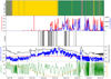 |
Fig. 3 Overview of the comet escort phase. First panel: main SDL/LDL mode operated by RPC-MIP per day: the anti-phased SDL sub-mode is represented in yellow, the phased SDL sub-mode in green, and the others mode (E1,E2 and LDL mode) in grey. Second panel: daily average of the number of cold electron signatures (blue line) and the ratio between the cold electron detection and the total number of measured spectra (red line). Third panel: location of the diamagnetic cavity crossings observed by the RPC-MAG fluxgate magnetometer. Fourth panel: the cometocentric distance of Rosetta (black line) and the electron-neutral collision dominated region (exobase) (blue point) expressed in km in logarithmic scale. The surface of 67P is shown by the red line. Fifth panel: Rosetta latitude (green line) expressed in degrees and the heliocentric distance (yellow line). |
3.3 Cold cometary electron detections as a function of the RPC-MIP operational SDL sub-mode
In this section, we report the detection of the double resonance in the RPC-MIP spectra for each SDL sub-mode. For the fourSDL sub-modes (Sect. 2.1), we report (i) the count of acquired mutual impedance spectra, (ii) the count of electron densities extracted from the spectra after the identification of the electron plasma frequency, (iii) the percentage of cold electron detections compared to the number of provided electron densities for a given SDL sub-mode and, (iv) the percentage of cold electron detections on the SDL sub-mode compared to the total cold electron detections for all SDL sub-modes. All of these parameters are listed in Table 1.
The E1 SDL sub-mode has been used only a few times (~2%) at the beginning of the cometary operations in 2014 August far from perihelion when Rosetta was far from 67P (~100 km). The total electron densities were not high enough (<100 cm−3) for a detection of the electron plasma frequency by RPC-MIP. Therefore, the E1 SDL sub-mode spectra do not enable to provide the electron plasma densities and therefore no cold electron detection.
The E2 SDL sub-mode has been used during the whole mission but only over short time periods (~1 h). The electron density has been extracted only in 6% of the E2 SDL sub-mode spectra and only few cold electron detections are observed (~1% of the density detections).
The anti-phased SDL sub-mode was the main mode operated from 2014 September to 2015 September (34% of the total acquired spectra). Over all the acquired spectra in this mode, only 11% enable to retrieve the total electron density and only 2% of spectra was shaped by a double resonance, characteristic for the presence of cold electrons. The cold electron detection for the anti-phased SDL sub-mode is concentrated close to perihelion (Fig. 3).
In 2015 September, the main mode was changed to the phased SDL sub-mode until the end of the mission in 2016 September (60% of total acquired spectra). This SDL sub-mode provided electron densities for about half of the acquired spectra and cold electron detections account for 23% of the spectra. This represents 95% of the total cold electron detections using the different RPC-MIP SDL sub-modes throughout the whole cometary phase of the Rosetta mission.
The anti-phased and the phased SDL sub-modes operated in almost the same ionospheric conditions in terms of heliocentric distance, cometocentric distance, latitude and neutral outgassing activity, leading to approximately the same conditions in terms of density and temperature for the warm electron population (Myllys et al. 2019). This means that the phased SDL sub-mode enables a better determination of the electron plasma frequency (i.e., the total electron density). The amplitude of the mutual impedance spectra around the electron plasma frequency is related to the Debye length λD. When the Debye length is small (high electron density or low electron temperature) compared to the transmitter-receiver distance (~20 cm), the main resonance close to the electron plasma frequency is clearly shaped. When the Debye length is large, of the order of (resp. larger than) the transmitter-receiver distance, the shape of the resonance is less visible (resp., flat) and the measurement of the electron plasma frequency can be challenging or even impossible.
The difference of the electron detections observed between the phased and anti-phased SDL sub-modes can be explained by the modeling of the mutual impedance spectra. Indeed, Wattieaux et al. (2019) modeled the mutual impedance spectra when RPC-MIP operated in phased SDL sub-mode and anti-phased SDL sub-mode in the same plasma conditions. They concluded that the signal-to-noise ratio is higher in phased SDL sub-mode, which enables to easily detect the resonances on mutual impedance spectra in this operating mode. Some examples of the modeling of the mutual impedance spectra in the anti-phased SDL sub-mode and in the phased SDL sub-mode are shown in Appendix B.2. As the total electron plasma frequency resonance in anti-phased SDL sub-mode can not always be identified, the resonance located close to the cold plasma frequency could sometimes be identified as the main resonance which thus leads in some cases to an overestimation of the total plasma density (around 20%). Moreover, the total electron density increased close to the perihelion due to the increase of outgassing activity (Hoang et al. 2017; Héritier et al. 2018). Assuming that the temperature of the electrons is constant (Myllys et al. 2019), the Debye length decreases close to the perihelion thus enabling RPC-MIP to detect more easily the total electron plasma frequency. Therefore, the two resonances are visible in the RPC-MIP spectra for both SDL sub-modes. This could explain the detection of the cold electrons in anti-phased SDL sub-mode close to the perihelion from 2015 July to 2015 September.
In conclusion, the RPC-MIP operational mode that maximises the cold electron detection is the phased SDL sub-mode, as shown by the observations and explained by the instrument modeling. Therefore, in the rest of this study we only focus on the cold electron observations in the mutual impedance spectra acquired in the phased SDL sub-mode. In the next section, we provide the characteristics of the cold cometary electrons from the RPC-MIP measurement.
Characteristics of the RPC-MIP dataset per operational SDL sub-mode (E1, E2, anti-phased and phased) for the whole cometary phase of the mission: (i) total count of acquired mutual impedance spectra, (ii) count of the extracted electron density from RPC-MIP spectra, (iii) percentage of cold electron detections for each SDL sub-mode and (iv) distribution of the cold electron detections.
4 Characteristics of the cold cometary electrons observed by RPC-MIP
In this section, we investigate the location of the cold cometary electrons depending on: (i) the latitude and the longitude (Sect. 4.1), (ii) the heliocentric distance (Sect. 4.2), (iii) the cometocentric and the exobase distances (Sect. 4.3), and, finally, (iv) inside the unmagnetized plasma (Sect. 4.4).
4.1 Cold cometary electron properties as a function of latitude and longitude
Figure 4 shows 2D longitude/latitude maps of the fraction of RPC-MIP spectra showing a signature of cold electrons compared to the total RPC-MIP spectra acquired (named cold-to-acquired ratio in the rest of the study) in the phased SDL sub-mode for two different periods. The first 2D-map (left panel) shows this ratio between 2015 September 4 and 2016 May 21 when thenorthern (resp. southern) hemisphere was in winter (resp. summer). The second panel shows the same ratio when the northern (resp. southern) hemisphere was in spring (resp. in autumn). For both panels, the ratio value is given by the color bar. For both periods, the cold electron detection in the southern hemisphere was higher than in the northern hemisphere, which corroborates the observation of a higher neutral outgassing activity in the southern hemisphere throughout the post-perihelion phase of the Rosetta escort phase at the comet (Hoang et al. 2017).
Moreover, Fig. 5 shows four histograms of the count of the total RPC-MIP spectra acquired in the anti-phased SDL sub-mode (black bars), the count of extracted electron density (red bars) and the count of RPC-MIP spectra with a cold electron signature (blue bars). Counts are plotted as functions of the cosine of the latitude (top panels) and of longitude (bottom panels). To ensure unbiased observation, we also plot the cold-to-acquired ratio (line of yellow squares). We note that the cold-to-acquired ratio increases with decreasing latitudes, independently from the season, going from 0.1 (sin (Latitude) = 1) to 0.6 (sin (Latitude) = −1).
The number of in situ acquired spectra is almost constant in longitude due to the rotation of the nucleus. The cold-to-acquired ratio is almost constant (~0.4) with a smooth maximum between − 90° and 0° and between 120° and 180°, when Rosetta was more or less above to the neck region of the comet (i.e., when the illuminated cross section of the comet was large) whatever the season. The maximum ratio of cold electrons detected by RPC-MIP (low latitude, longitude corresponding to the neck region) can be compared with the map of the H2 O density (Hoang et al. 2017; Kramer et al. 2017). The maximum of neutral molecule density corresponds to the maximum of cold electrons detections by RPC-MIP. Therefore, the cometary cold electrons shall be associated to electrons thermalized by collisions with the cometary neutrals. However, this assumption needs to be counterbalanced by the fact that during the final part of the cometary operations, the electrons born close to the nucleus were not expected to have time to cool down before reaching the spacecraft where they are observed(Engelhardt et al. 2018). We detail in Appendix A the expected number of electron-neutral collisions for electrons that are moving radially away from the comet nucleus, in a ballistic way, and we show that such newborn electrons could not suffer enough collisions to be observed as cold electrons at the spacecraft location. Instead, the observations of cold electrons by RPC-MIP reported in this study are consistent with the existence of a trapped population of electrons in the inner come region, because of the effect of an ambipolar electric field. The presence of such an electric field is supported by full kinetic cometary plasma simulations that captures the electron kinetic dynamics (Deca et al. 2017, 2019) and where evidence of trapped electrons is observed (Sishtla et al. 2019). The cooling process is expected to be much more efficient for trapped electrons than for passing (or ballistic) electrons because the former travel much longer distances within the denser cometary neutral regions (Eriksson et al. 2017). This would explain why, once transported away from the comet nucleus, cold electrons can also be observed, even when the comet is far from perihelion and the number of collisions predicted from an oversimplified ballistic motion only (i.e., without any trapping process) is expected to be low.
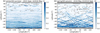 |
Fig. 4 Maps of the fraction of RPC-MIP spectra showing a cold electron signature compared to the total RPC-MIP spectra acquired in phased SDL sub-mode. Left panel: 2D longitude/latitude map from 2015 Sept 4 to 2016 May 21 when the southern (resp. northern) hemisphere was in summer (resp. winter). Right panel: 2D longitude/latitude map from 2016 May 22 to 2016 Sept 30 when the southern (resp. northern) was in autumn (resp. spring). The color bar gives the cold-to acquired ratio measured by RPC-MIP from 0 to 1 (white to blue). Grey corresponds to non-detection areas. |
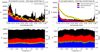 |
Fig. 5 Histograms of the count of RPC-MIP cold electron signatures (blue bars), the count of derived RPC-MIP electron densities (red bars) and the total count of mutual impedance spectra acquired in the phased SDL sub-mode (black bars) compared to the sine of the latitude (top panels) and the longitude expressed in degrees (bottom panels). The cold-to-acquired ratio is shown in yellow squares. Left panels: from 2015 Sept. 4 to 2016 May 21 corresponding to the southern (resp. northern) hemisphere in summer (resp. winter). Right panels: from 2016 May 22 to 2016 Sept. 2016 corresponding to the southern (resp. northern) hemisphere in autumn (resp. spring). |
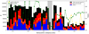 |
Fig. 6 Histogram of the count of cold electron detections by RPC-MIP (blue bars), the count of RPC-MIP electron density measurement (red bars) and the count of mutual impedance spectra acquired in phased SDL sub-mode (black bars) as function of the heliocentric distance expressed in AU. The cold-to-acquired ratio is shown as a line of yellow squares. The line of green squares shows the fraction of time where Rosetta was in the southern hemisphere. Heliocentric distances corresponding to Rosetta nightside excursion are shaded in grey. |
4.2 Cold electrons as a function of the heliocentric distance
The neutral outgassing activity evolves with the distance from the Sun (Hansen et al. 2016) with a maximum located at perihelion (2015 August) when 67P was at 1.24 AU and decreased gradually when 67P moved away from the Sun. At the end of the comet escort phase, 67P was at 3.8 AU from the Sun. Figure 6 shows an histogram of the counts of the total in situ RPC-MIP spectra acquired in phased SDL sub-mode (black bars), the counts of extracted electron density (redbars) and the counts of RPC-MIP spectra presented a cold electron signature (blue bars). All of the bars dependon the heliocentric distances expressed in AU. RPC-MIP observed cold electrons at all heliocentric distancesfrom 1.25 AU, close to the perihelion, to 3.8 AU at the end of the cometary escort phase but with strong fluctuations as shown by the cold-to-acquired ratio (yellow line). Close to 2.7 AU, the detection of cold electrons decreases due to the fact that Rosetta was far from the comet (nightside excursion, shaded in grey). Moreover, during the last part of the comet escort phase (from 3.2 AU), RPC-MIP switched from burst mode (~3.5 s between two successive measurements) to normal mode (~30 s), explaining the decrease in the number of acquired RPC-MIP spectra. For each bar, we also computed the ratio of the period when Rosetta was above the southern hemisphere. This ratio is plotted as a line of green squares. Between 1.24 AU and 3.2 AU, a strong correlation is found between the RPC-MIP cold electron detections and the fact that Rosetta was in majority above the southern hemisphere (south-to-total latitude >0.5). Therefore, the variability of the cold electron detections in heliocentric distance seems to be mainly related to the latitude and thus to the outgassing activity.
From August 2016, Rosetta described elliptical orbits with a periapsis located in the southern hemisphere (see Fig. 3). However, taking into account the observations in function of the cometocentric distance during the whole period (June-September 2016), Rosetta navigated insouthern hemisphere as much as in northern hemisphere from 2 to 15 km, corresponding to a south-to-total ratio around 0.5 (right bottom panel). Therefore, the effect of the cometocentric distance can be disentangled from the latitude effect in the observation of cold electrons.
4.3 Cold electrons as a function of the cometocentric distance
Previous studies from RCP-MIP and RPC-LAP have shown that the total electron density varies as 1∕r67P where r67P is the cometocentric distance (Edberg et al. 2015; Henri et al. 2017; Héritier et al. 2018). Myllys et al. (2019) showed that the warm electrons measured by the RPC-IES, corresponding to the ones observed by RPC-LAP, similarly vary with the cometocentric distance. Figure 7 shows four histograms of the counts of RPC-MIP acquired spectra (black bars), the counts of RPC-MIP spectra for which the total electron density has been extracted (red bars) and the counts of the RPC-MIP spectra for which a mix of cold and warm electrons has been observed (blue bars) in the phased SDL sub-mode as function of the cometocentric distance expressed in km. The cold-to-acquired ratio is also shown as a line of yellow squares, together with the fraction of times where Rosetta was in the southern hemisphere as a line of green squares. Each histogram corresponds to a different heliocentric distances range.
Close to perihelion (from 1.3 to 1.9 AU, corresponding to the period from 2015 September 12 to 2015 December 16, left-top panel), Rosetta navigated far from the comet from 100 to 1500 km (only the part of the histogram up to 600 km is shown). As described in the previous section, the cold electron detections were more frequent when Rosetta was in the southern hemisphere, also visible in the histogram for a cometocentric distance around ~150 km and from 200 to 300 km. Therefore, the variation of cold electron detection is mainly due to the latitude and not due to the cometocentric distance. The cold electrons are detected far from the comet when Rosetta was farther than 500 km from the nucleus. However, the cold-to-acquired ratio tends to decrease when Rosetta moves away from the nucleus. Indeed, this ratio ranges from 0.5 at around 100 km to 0.05–0.1 at around 600 km. This observation suggests that the cold electron density also decreases with the distance to the nucleus.
When 67P travelled from 1.9 to 2.6 AU (17 December 2015 to 17 March 2016), Rosetta was closer to the nucleus that is, between from 20 and 100 km (right top panel). The effect of the higher outgassing activity in the summer hemisphere is also observed around 25 km with a maximum of cold electrons detection when Rosetta was mainly in the southern hemisphere and a minimum around 30 km when Rosetta was in the northern hemisphere. As observed previously, the cold-to-acquired ratio tends to 0 as the cometocentric distance increases. Similar observations can be made when the comet was between 2.6 to 3.2 AU.
During the last part of the cometary escort phase from 3.2 to 3.8 AU (14 June 2016 to 30 September 2016), when Rosetta was at the closest distance to the nucleus until the final descent (Taylor et al. 2017), we see that the cold-to-acquired ratio clearly decreases when the cometocentric distance increases. From 2 to 15 km, Rosetta navigated at all latitudes, that corresponds to a south-to-total ratio around 0.5 (right bottom panel). Therefore, the observation of the cold electrons is less biased by the higher outgassing activity in the summer hemisphere. Thus, the decrease of the cold electron observations could be due to the fact that the total electron density decreases when Rosetta was far from the comet (Edberg et al. 2015; Odelstad et al. 2015).
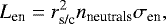
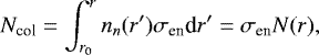
In this study, we also investigated the cold electron observations with respect to the distance of the electron exobase where below this distance, the electron-neutral collisions are supposed to be frequent (Mandt et al. 2016). The exobase distance Len has conventionally been defined as follows:
 (2)
(2)
where σen is the electron-neutral cross-section for 5 eV electrons on water molecules σen ≃ 5 × 10⁻¹⁶ cm2 (Itikawa & Mason 2005), rs/c is the distance of the spacecraft from the nucleus and nneutral is the neutral density at the spacecraft location given by the ROSINA COmet Pressure Sensor (COPS) instrument (Balsiger et al. 2007). The exobase distance is shown in Fig. 3 in blue points for the whole cometary escort phase of the mission. The 2 km limit (red horizontal line) indicates the comet surface. No collisional cooling is expected when the electron exobase distance Len is less than the nucleus size of about 2 km meaning that no collisional region is formed. Therefore, this region was only formed close to perihelion from 2015 March to 2016 March, which means that no cold electrons should be created outside this period. Moreover, from 2016 March to 2016 September, the CO2 molecule dominated the neutral outgassing (Gasc et al. 2017; Héritier et al. 2018). The cross-section of the CO2 molecule for 5 eV electrons is equal to 4.58 × 10⁻¹⁶ cm2 that is almost the same as for H2O (Itikawa 2002). Therefore, the dominance of carbon dioxide in the southern hemisphere during the last part of the mission can not explain the fact that cold electrons were also observed far from perihelion.
Figure 8 shows a scatter plot of the electron exobase distance computed with σen for the H2 O molecule compared to the cometocentric distance of Rosetta all expressed in km. The blue points indicate the presence of cold electrons from the RPC-MIP spectra and grey points all spectra acquired in phased SDL sub-mode. The blue line shows the surface of 67P taken at 2 km. The red line corresponds to the case where Len is equal to rs/c. First, the cold electrons are observed for all distances of the electron exobase from 0.1 to 1000 km, especially when the electron-neutral collision-dominated region is not supposed to have formed (< 2 km) which is shown on the left of the blue vertical line in Fig. 8. Second, the cold electrons have been detected by RPC-MIP most of the time outside the region where the electron-neutral collisions are frequent. These observations, made when Rosetta was most of the time outside this region, would have benefited from a confrontation at closer heliocentric distances. Unfortunately, because of spacecraft safety measures, few Rosetta observationshave been taken closer to the nucleus, below the electron exobase, when outgassing activity was high.
Finally, we shall emphasize various limits in the model used here. First, the distance of the exobase, as given in Eq. (2), is obtained from an idealized toy model assuming spherical symmetry, in order to provide a simplified boundary definition separating a region around 67P dominated by electron-neutral collisions from an outer collisionless region. The electron energy has been taken at 5 eV that is not representative of the whole electrons energy range. Therefore, this boundary could actually vary of about an order of magnitude, depending on actual electron temperature. Second, the model does not take into account the fact that the cometary outgassing activity monitored by Rosetta has been observed to be strongly asymmetrical (Hässig et al. 2015), which is expected to directly affect electron-neutral collisional processes close to the surface, where they are expected to be more frequent.
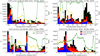 |
Fig. 7 Histograms of the count of cold electron detections by RPC-MIP (blue bars), the count of RPC-MIP electron density measurement (red bars) and the count of mutual impedance spectra acquired in phased SDL sub-mode (black bars) as a function of the cometocentric distance expressed in km. The cold-to-acquired ratio is shown as a line of yellow squares. The line of green squares shows the fraction of time where Rosetta was in the southern hemisphere. Each histogram ismade for a different range of heliocentric distances. |
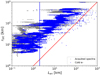 |
Fig. 8 Distance of the electron exobase Len compared to the cometocentric distance of Rosetta rs/c. The colored data shows the cold electrons detected by the double resonance on the RPC-MIP spectra and the grey data shows all acquired spectra in phased SDL sub-mode. The red line shows where rs/c = Len and the blue vertical line shows the surface of 67P defined at around 2 km. |
4.4 Observations of cold cometary electrons inside diamagnetic cavity
The diamagnetic cavity is defined as zero-magnetic-field region, formed when the magnetic field from the solar wind can not reach the nucleus (Goetz et al. 2016b). With the absence of an intrinsic magnetic field of the comet, the ambient magnetic field is then zero. This region has been observed sporadically during the comet phase. The RPC-MAG fluxgate magnetometer identified 665 diamagneticcavity crossings from 2015 April to 2016 February (Goetz et al. 2016a). The physics of the region is still under debate but Odelstad et al. (2018) showed that cold electrons were almost always observed in large amounts inside the diamagneticcavity. Edberg et al. (2019) found that the observations of cold electrons in the diamagnetic cavity were organized by the direction of the solar wind convective electric field. More cold electrons were observed in the − Econv hemisphere that was the main direction inside the diamagnetic cavity.
Figure 9 shows the total number of RPC-MIP acquired spectra (line of black squares), the spectra from which the total electron density has been extracted (line of red squares) and the spectra containing cold electrons signatures (line of blue squares) inside each diamagnetic cavity crossing when RPC-MIP operated in phased SDL sub-mode versus the cavity index (in chronological order, given by Goetz et al. (2016a)). The cold-to-acquired ratio for each diamagnetic cavity crossing is shown in yellow points. When RPC-MIP mainly operated in the phased SDLsub-mode (Sect. 3.3), the fraction of cold electrons observed by RPC-MIP is close to 1 (~0.89) which indicates that the RPC-MIP observed most of the time cold electrons inside the diamagnetic cavity, which is consistent with the observationsby RPC-LAP (Odelstad et al. 2018). However, for the diamagnetic cavity crossings measured by RPC-MAG between 21 to 26 December 2015 (indices 610-650), the fraction of cold electrons detected by RPC-MIP decreases to ~0.10 even thoughthe RPC-MIP operated in phased SDL sub-mode. Inside the diamagnetic cavity, RPC-MIP was able to derive the total electron density, but the resonance due the presence of the cold electrons has not been detected. This can be indicating different plasma conditions, especially in the limit where the warm-to-cold temperature ratio is not large enough (< 30) or the cold-to-total density ratiois too low (<0.6) (see Sect. 3.1).
5 Comparison with RPC-LAP measurements and discussions
By evaluating the slope of the measured current-voltage curves (hereafter I-V curves), the two Langmuir probes were able to detect and characterize the cold electron population (Eriksson et al. 2017). First, we compare the observations of cold electrons between the Langmuir probes and the mutual impedance experiment (Sect. 5.1). Second, we discuss the observations of the cold electron population by RPC-MIP during the end of cometary operations (Sect. 5.2).
5.1 Comparison of the detection capabilities between RPC-LAP and RPC-MIP
Engelhardt et al. (2018) showed that a high value of the RPC-LAP I-V curve slope (>70 nA/V) characterized the presence of cold electrons in the surrounded plasma. The electron slope of the I-V curve depends on the electron density and the electron temperature. When the electron density is measured simultaneously by RPC-MIP, it is then possible to constrain the electron temperature.
Eriksson et al. (2017) reported the first in situ observation of cold electrons by RPC-LAP with the I-V curve and Engelhardt et al. (2018) extended this study for the whole cometary phase of the Rosetta mission. They derived values of each electron slope when RPC-MIP electron density was available. From 388 900 slopes measured by the Langmuir Probes during the cometary phase, 49 539 slopes (~12.7%) showed the presence of cold electrons mainly close to the perihelion (Engelhardt et al. 2018).
In order to compare the signature of cold electrons by the two instruments, we focus on RPC-MIP SDL phased sub-mode (main mode from 2015 September to 2016 September, see Sect. 3.3), with simultaneous RPC-LAP measurements, resulting in 124 245 slopes among which 7876 slopes (~6%) indicated the presence of cold electrons.
In the following, we take into account the fact that the cadence of the RPC-MIP measurement was higher than the RPC-LAP measurement (~3.5 s for RPC-MIP and ~1–3 min. for RPC-LAP). We computed the fraction of RPC-MIP spectra containing cold electrons between two consecutive RPC-LAP measurements. The result is shown in Fig. 10 by two histograms. The left panel shows the RPC-MIP cold-to-acquired ratio between two consecutive RPC-LAP measurements when RPC-LAP observed cold electrons. For the 7876 slopes measured by RPC-LAP indicating a presence of cold electrons, RPC-MIP observed cold electrons, over at least one RPC-MIP spectrum between two measurements of RPC-LAP, in ~99.2% (i.e., for 7814 slopes). Moreover, in such cases, the RPC-MIP cold-to-acquired ratio is rather large, with an average value of 0.62. For almost 20% of the RPC-LAP measurements with cold electrons, RPC-MIP observed cold electrons for all acquired spectra between the two RPC-LAP measurements. Therefore, RPC-MIP measured cold electrons when RPC-LAP observed cold electrons. Second, the right panel in Fig. 10 shows the RPC-MIP cold-to-acquired ratio when RPC-LAP did not observed cold electrons (65 459 slopes). This ratio is lower than the previous case. The mean value is equal to 0.3 with ratio values often lower than 0.1. This observation can be explained by the fact that the signature of cold electrons is less straightforward for both instruments. Several explanations are possible. First, the cold electrons could be observed as a pulse during just a few seconds might not have been resolved by the lower time resolution of RPC-LAP. Second, the plasma conditions could be close to the detection limits of the two instruments for cold electrons.
In the following, we focus on the measurements acquired simultaneously (~1 s) between the two instruments, when RPC-MIP operated in phased SDL sub-mode. 33 850 measurements were performed simultaneously between the two instruments. The cold electrons have been observed by both instruments for 2106 measurements, which represents ~6% of such measurements. In total, RPC-MIP observed cold electrons for 8605 measurements (~26% of the total measurements), while RPC-LAP observed cold electrons for 3092 measurements (~9% of the total measurements). For each measurement, we extracted the total electron density provided by RPC-MIP and the electron slope provided by RPC-LAP. Figure 11 shows a scatter plot of both parameters. The measurements are subdivided in three cases: RPC-LAP and RPC-MIP both observed cold electrons (blue points), RPC-LAP observed cold electrons while RPC-MIP did not (green points), and RPC-MIP observed cold electrons while RPC-LAP did not (red points). Regarding the total electron density measured by RPC-MIP, when the electron density is high (around about 1500–2000 cm−3), the number of cases where RPC-LAP did not observe cold electrons but RPC-MIP did increases. This can be explained by the spacecraft potential preventing cold electrons from reaching the RPC-LAP probes. For the case where RPC-LAP observed cold electrons and RPC-MIP did not (green points), the electron density measured by the RPC-MIP is lower than 1000 cm−3. By analysing the RPC-MIP spectra for this case, we found three typical kinds of spectra. First, some typical spectra are shaped by a double resonance indicating the presence of cold electrons but below the detection threshold of the automatic extraction algorithm pointing out that cold electron signatures are also hidden in the RPC-MIP data at lower frequencies. Second, the cold electron peak could have been removed by the automatic interference removal process: the RPC-MIP spectra is sometimes shaped by only one resonance located close to two well-known interferences which are treated by boldly removing the contaminated frequency channels and interpolating the spectrum afterwards. Thus, one of the two resonance may have ended up in one of the two deleted frequency channels too. Third, the last typical spectrum shows a very low signal-to-noise ratio. Therefore, the RPC-MIP is at the limit of the detection capabilities of the electron measurements (due to a too large Debye length compared to the RPC-MIP transmitter-receiver distance).
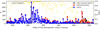 |
Fig. 9 Count of cold electron detections by RPC-MIP (line of blue squares), count of electron density derivation (line of red squares) and count of acquired mutual impedance spectra (line of black squares) for each diamagnetic cavity crossing when RPC-MIP operated in phased SDL sub-mode. The ratio of RPC-MIP cold electron detections with the total acquired mutual impedance spectra is shown in yellow points. |
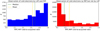 |
Fig. 10 Histograms of the cold electron detections by RPC-MIP normalized by the total in situ RPC-MIP acquired spectra for the time periods where (i) the RPC-LAP observed cold electrons (first panel) and where (ii) the RPC-LAP does not observed cold electrons (second panel). All are obtained when the RPC-MIP operated in SDL phased sub-mode. The mean (yellow vertical bar) and the median (green vertical bar) of the ratio are also shown in the two histograms. |
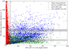 |
Fig. 11 Scatter plot of all simultaneous measurements (RPC-MIP and RPC-LAP measurements where made within 1 sec, considering only RPC-MIP phased SDL sub-mode) showing RPC-MIP total electron density, expressed in cm−3 versus the RPC-LAP I-V curve slope, expressed in nA/V. Measurements are subdivided in three cases: RPC-LAP and RPC-MIP both observed cold electrons (blue points), RPC-LAP observed cold electrons while RPC-MIP did not (green points) and RPC-MIP observed cold electrons while RPC-LAP did not (red points). The grey horizontal bars indicate the electron density corresponding to the well-known RPC-MIP interferences (see Sect. 2.2). |
5.2 Discussion
We have reported in this study that the RPC-MIP detected cold electrons in the inner coma of comet 67P, thus confirming previous independent observation from RPC-LAP (Eriksson et al. 2017; Engelhardt et al. 2018). However, thanks to the higher measurement rate during end of cometary operations, RPC-MIP reported a significantly larger quantity of cold electrons, associated to transient cold electron bursts occurring on timescales of minutes or faster. Engelhardt et al. (2018) showed that the cold electrons were generally observed when the outgassing activity was high that is, close to perihelion from 2015 July to 2015 September. This result was consistent with the existence of a region dominated by electron-neutral collisions (Mandt et al. 2016). However, Engelhardt et al. (2018) showed that the cold electrons were also observed in minority during the last months of the cometary operations. To explain the observations of cold electrons at large heliocentric distance, they suggested the presence of an ambipolar electric field that keeps the electrons in the inner coma for a long time after the collision with the neutrals. The presence of an ambipolar electric field suggested by previous studies (Vigren et al. 2015; Madanian et al. 2016), is supported by large-scale modeling of the cometary environment of 67P (Deca et al. 2017). The RPC-MIP observations reported in this study show that cold electrons observations were statistically correlated to regions of high outgassing activity, independently from heliocentric or cometocentric distances, and confirms the observation of cold electrons at large heliocentric distances.
Figure 12 shows (i) a map of the cold-to-acquired ratio, (ii) a map of the neutral density given by ROSINA-COPS and, (iii) a map of the total electron density retrieved by RPC-MIP depending on the latitude and the cometocentric distance from 2016 August 2 to 30. During this period, Rosetta made several orbits around the nucleus close to the cometary surface (from 5 km to 16 km), where spherical symmetry can no longer be assumed. Almost all latitudes have been visited from −80° to 80°. The neutral density was still high in the southern hemisphere at this period (Gasc et al. 2017). In this low outgassing activity situation and at low altitude, cold electrons (left panel) are observed locally above the surface, namely where the strongest neutral outgassing occurs (e.g. latitude −50 deg). However, during some orbits, such a high neutral outgassing is observed while cold electrons signatures are not (e.g. latitude −50 deg, distance 6.5 km). Therefore, even if a strong neutral density clearly appears to be necessary to simultaneously observe cold electrons signatures, it does not appear to be a sufficient condition, so that there is no one-to-one relation between both observations, at least with the detection method used in this work based on the spectral double resonance signature. The influence of the ambipolar electric potential, associated to the cometary plasma inhomogeneities and localized around the comet nucleus, in terms of particle trapping, might facilitate the electron cooling. This hypothesis shall be investigate in further details from global modeling (Deca et al. 2017, 2019; Sishtla et al. 2019) to investigate the physical processes at the origin of the cold electron population far from perihelion reported in this study.
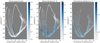 |
Fig. 12 First panel: map of the cold-to-acquired ratio compared to the latitude and the cometocentric distance. Second panel: map of the neutral density, expressed in cm−3, given by ROSINA-COPS compared to the latitude and the cometocentric distance. Third panel: map of the total electron density, expressed in cm−3, retrieved byRPC-MIP compared to the latitude and the cometocentric distance. The data are given from 2016 August 2 to 30. |
6 Conclusion
Initially designed to assess the core cometary electron population in the ionosphere of the comet 67P/Churyumov-Gerasimenko, the mutual impedance probe RPC-MIP onboard the Rosetta orbiter detected a mix of warm and cold cometary electrons (Tw ~ 5 eV, Tc ~ 0.1 eV). In plasma conditions characterized by two isotropic Maxwellian electron populations dominated by the cold electron component (from 60 to 90%) of the totaldensity) and with a large enough electron temperature ratio (> 30), the acquired mutual impedance spectra exhibit a characteristic double resonance signature. This characteristic has been predicted by modeling the instrument response of the mutual impedance probe RPC-MIP with a variety of models, ranging from an idealized mutual impedance probe (Gilet et al. 2017) to, more recently, a model taking account both the spacecraft geometry and the presence of a large ion sheath surrounding the instrument (Wattieaux et al. 2019).
In this study, we have focused on cometary regions characterized by a mix of electron populations dominated by the cold electron component, that was sporadically observed by RPC-MIP. In this purpose, we have investigated the in situ mutual impedance spectra exhibiting a well-defined double resonance, for the whole cometary escort phase from 2014 August to 2016 September. We have shown that the RPC-MIP cold cometary electrons detection capability strongly depends on the operational mode of the instrument.
Focussing on the most sensitive RPC-MIP operational mode for cold electron detection (the so-called phased SDL sub-mode), during the period Sept. 2015–Sept. 2016, RPC-MIP significantly observed a dominance of the cold electron population in the southern hemisphere, where the neutral outgassing activity was higher during post-perihelion (Hoang et al. 2017; Kramer et al. 2017; Läuter et al. 2019). These RPC-MIP observations are consistent with a model where the electrons have been cooled by collisions with the neutral outgassing activity from the nucleus. Moreover, regions dominated by a strong cold electron component have been observed at all heliocentric distances, from 1.25 AU, close to the perihelion, to 3.8 AU at the end of the cometary operations. The observation of cold electrons far from theSun is not in agreement with the fact that the electron-neutral collision dominated region around the comet isconsidered to be absent at large heliocentric distances (Mandt et al. 2016). Instead, the reported observationsshow that the collisional electron cooling seems to be more efficient that previously expected and suggests that the estimation of the electron exobase must be revisited in order to fit the observations reported in this study.
We have also performed a comparison of the occurence of a mixed of cold and warm electrons provided by the measurement of the Langmuir probe RPC-LAP in the ionized environment of comet 67P (Eriksson et al. 2017; Engelhardt et al. 2018) and confirm these observations by using a completely independent instrumental method. For instance, inside the diamagnetic cavity (i.e., unmagnetized region), RPC-MIP observed cold electrons most of the time, which is in good agreement with previous observations made by RPC-LAP (Odelstad et al. 2018). Thanks to this comparison, we have showed that RPC-MIP is generally more sensitive to the cold electrons than RPC-LAP, presumably because RPC-MIP is less affected by the spacecraft potential due to the fact that RPC-MIP is not a local measurement of the plasma parameters of the electrons. On top of that, we also reported observations of cold-electrons-dominated structures on smaller time and length scales: of the order of seconds, corresponding to structures of few kilometers in size. This is particularly seen in the last part of the mission from 2016 April to 2016 September when the outgassing activity was low.
Finally, we stress that the absence of a double resonance, observed in the RPC-MIP mutual impedance spectra and used in this study to access regions characterized with a strong majority of cold enough electrons (i.e. the regime of plasma parameters where the cold-to-total density ratio is from 0.6 to 0.9 and for a warm-to-cold temperature ratio higher than ~30), is not necessarily associated to the absence of cold electrons. Indeed, cold electrons can be present without a double resonance signature in the mutual impedance spectra, for instance in the case of a smaller cold-to-total density ratio. This is well modeled and reported in Wattieaux et al. (2019), that developed a model of the mutual impedance response taking into account the effect of the spacecraft charging on the mutual impedance measurement. By fitting the in situ mutual impedance spectra to a dataset of modeled mutual impedance spectra in a two-electron temperature plasma, it has been shown that it is possible to detect the presence of cold electrons even when the double resonance is not visible on the mutual impedance spectra (Wattieaux et al. 2020).
Acknowledgements
This work was supported by CNES and by ANR under the financial agreement ANR-15-CE31-0009-01. We acknowledge the financial support of label ESEP (Exploration Spatiale des Environnements Planétaires). The authors benefited from the use of the cluster Artemis (CaSciModOT) at the Centre de Calcul Scientifique en région Centre-Val de Loire (CCSC). Part of this work was inspired by discussions within International Team 402: “Plasma Environment of Comet 67P after Rosetta” and International Team 336: “Plasma Surface Interactions with Airless Bodies in Space and the Laboratory” at the International Space Science Institute, Bern, Switzerland. MR acknowledges the State of Bern and the Swiss National Science Foundation (SNSF, 200020_182418). The Rosetta RPC-MIP mutual impedance spectra are publicly available on the ESA Planetary Science Archive (PSA).
Appendix A Estimation of the number of collisions undergone by an electron
In Sect. 4, we have demonstrated that the number of cold electron observations strongly correlates with a high neutral gas production. Moreover, in Sect. 5.2, we showed that at the end of the operations, cold electrons were observed while the neutral gas production was low. In order to understand when the electrons can be cooled by collision with neutrals, we have computed an estimation of the number of collisions undergone by an electron moving radially and ballistically between the comet surface and the spacecraft location for different observational conditions depending on the outgassing activity and the spacecraft cometocentric distance r. In order to estimate the number of collisions undergone by that electron before reaching the spacecraft, we computethe number of neutral molecules in a cylinder going from the cometary surface at radius r0 to the spacecraft location:
 (A.1)
(A.1)
where σen is the electron-H2O collision cross-sectionand N(r) is the neutral column density between the surface and the spacecraft location that can be expressed as follows:
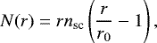 (A.2)
(A.2)
with nsc is the neutral density measured by the ROSINA/COPS instrument at the spacecraft location and where we have considered a neutral density decaying in 1∕r2 (Mandt et al. 2016). Note that the water molecules were dominant in the cometary ionosphere until March 2016 (Gasc et al. 2017), while CO2 dominated the ionosphere at the end of the cometary operations. However, cross-sections for electron collisions are of the same order of magnitude for both molecules, so that we need not care much about the actual neutral composition in this computation (Itikawa 2002; Itikawa & Mason 2005). We have also computed the outgassing rate Q which for a spherically symmetric gas
flow at constant speed is defined as follows (Hansen et al. 2016):
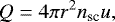 (A.3)
(A.3)
where u is the neutral gas radial velocity that we have fixed at 1 km s−1. Figure A.1 shows the number of electron-neutral collisions defined by the colorbar (red = 0, blue = 20) depending on the outgassing rate Q and the cometocentric distance of the spacecraft. We have included the conditions encountered by the spacecraft at different times of the operations: (i) close to the perihelion (15 Sept. and 15 Dec. 2015, blue square and circle) when the outgassing activity was high and the spacecraft was far from the nucleus (ii) in March 2016 when the outgassing activity decreased and the exobase was expected to have not formed, and, finally, (iii) close to the end of the operations in August 2016 (shown by the black points). Note that the data are shown only when the RPC-MIP operated in phased SDL sub-mode. First, from the perihelion to March 2016, we expect that an electron, that appears close to the cometary surface and moves radially and ballistically away from the nucleus, underwent at least one collision far from the nucleus where the spacecraft was located during this period. This is equivalent to the definition of the electron exobase (Sect. 4). Moreover, at least one electron-neutral collision is still expected at medium outgassing activity close to the nucleus (around 10 km), which is consistent with the observations of cold electrons made by RPC-MIP. Second, from March 2016 to the end of the operations when the outgassing activity was low, no electron-neutral collisions were expected despite the fact that the spacecraft was getting closer to the nucleus. Therefore, the observation of cold electrons by RPC-MIP at the end of the Rosetta cometary operations is not consistent with the cooling of newborn electrons that are ballistically escaping the inner coma region, but is rather consistent with electron that would stay longer in the denser inner cometary atmosphere region, and therefore with electrons that got trapped in the inner coma by the ambipolar electric field as shown in recent kinetic simulations of cometary electron dynamics (Deca et al. 2017, 2019; Sishtla et al. 2019).
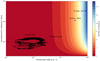 |
Fig. A.1 Number of expected collisions (shown by the colorbar) undergone by an electron born at the nucleus surface, moving radially away from the nucleus and ballistically, before reaching the spacecraft location, depending on the outgassing rate, expressed in s−1, and the spacecraft-comet distance, expressed in km. The conditions encountered by Rosetta between 1st and 15th August 2016 are given by the black points. |
Appendix B Mutual impedance spectra modeled in a two-temperature electron plasma
In this appendix, we detail the computation and the modeling of the mutual impedance spectra corresponding to the RPC-MIP experiment. The computation of the electrostatic potential induced by a transmitting electrode and the mutual impedance in a two-temperature electron plasma is explained in Appendix B.1. As stated in Sect. 3.1, in some plasma conditions, the synthetic mutual impedance spectra exhibit a double resonance which enables to detect the presence of cold electrons in the cometary plasma. In Appendix B.2, we provide some examples of the synthetic mutual impedance spectra modeled in a two-temperature electron plasma, showing a clear double resonance and enabling to constrainthe plasma conditions where the double resonance can be clearly seen on the acquired RPC-MIP spectra.
B.1 Computation of the electrostatic potential in a two-temperature electron plasma
We considera collisionless and unmagnetized two electron temperature plasma, modeled as a superposition of two isotropic Maxwellian EVDF. This plasma is characterized by four parameters: nw, nc, Tw and Tc which are respectively the electron density of the warm and cold electrons with their corresponding electron temperatures. The total electron density given by RPC-MIP is noted ne. The total plasma frequency is defined as 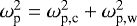 with the cold and warm plasma frequencies
 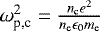 and
and 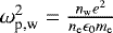 , and the cold and warm Debyelengths
  ,
,  .
.
In an isotropic and homogeneous plasma, the potential ϕ induced by a pulsating point charge Qexp(iωt), at frequency ω and at a radial distance d from the charge (Chasseriaux et al. 1972) is given by:
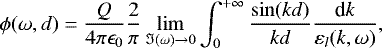 (B.1)
(B.1)
where εl is the longitudinal dielectric function of the plasma, k the wavevector and ɛ0 the vacuum permittivity. For a sum of two isotropic Maxwellian EVDF, the dielectric function is given by:
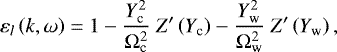 (B.2)
(B.2)
where:
![Mathematical equation: \[ \Omega_{\textrm{c}} = \frac{\omega}{\omega_{\textrm{p,c}}} \text{ and } \Omega_{\textrm{w}} = \frac{\omega}{\omega_{\textrm{p,w}}} \]](/articles/aa/full_html/2020/08/aa37056-19/aa37056-19-eq16.png)
![Mathematical equation: \[ Y_{\textrm{c}} = \frac{\Omega_{\textrm{c}}}{\sqrt{2\mu / \tau}K} \text{ and } Y_{\textrm{w}} = \frac{\Omega_{\textrm{w}}}{\sqrt{2}K} \mathrm{~with~} K = k\ \lambda_{\textrm{D,w}}, \]](/articles/aa/full_html/2020/08/aa37056-19/aa37056-19-eq17.png)
and the ratio of the two temperatures and densities, resp.  and
and  . The function, Z′, is the first derivative of the plasma dispersion function Z (Fried & Conte 1961). We use the method detailed in Gilet et al. (2017, see Sect. 3 and Appendix A for details regarding the numerical method) to compute the integral in Eq. (B.1), needed to model the electrostatic potential at the receiver positions.
Three models of the RPC-MIP instrument response have been implemented using the electrostatic potential computed in a two-temperature electron plasma. Model 1 is a simplified RPC-MIP geometry considering each emitter as a pulsating point charge. This method, detailed in Gilet et al. (2017), is used to characterize the effect of the electron velocity distribution function on the instrument response (Chasseriaux et al. 1972; Béghin 1995; Gilet et al. 2019). Model 2 implements the discrete-surface-charge-distribution (DSCD) method developed by Béghin & Kolesnikova (1998), adapted to the RPC-MIP experiment by Geiswiller et al. (2001) and coupled to the electric potential in a two-temperature electron plasma described above. This method enables to take into account the spacecraft geometry and the spacecraft charging on the modeling of the mutual impedance measurement. Model 3, developed by Wattieaux et al. (2019), adds in the previous model the effect of the spacecraft charging, especially the plasma inhomogeneity (plasma sheath) around the RPC-MIP experiment to model this effect.
Finally, we note that the RPC-MIP mutual impedance spectra are obtained for frequencies much above the electron cyclotron frequency (<1 kHz), in the so-called electrostatic frequency range. In this range, the plasma oscillations of interest are mainly the electron acoustic and Langmuir oscillations, which are both electrostatic oscillations, whose dispersion depends essentially on the parallel temperature. In the case of electron temperature anisotropies, the mutual impedance spectra would mostly monitor the parallel temperature(s). We applied these models to characterize the measurement made in phased and anti-phased SDL operational sub-modes of the RPC-MIP experiment, and to identify the plasma conditions under which a double resonance shapes the RPC-MIP spectrum. A comparison of the three model results is given in the following section.
B.2 Modeling of the expected RPC-MIP mutual impedance spectra
Figures B.1–B.3 show modeled mutual impedance spectra for different cold-to-total density ratio and temperature ratio in the anti-phased SDL sub-mode (purple line) and in phased SDL sub-mode (black line) modeled by Model 1, Model 2, and Model 3 respectively. The warm-to-cold electron temperature ratio, noted τ, increases from left to right, while the cold-to-totaldensity ratio, noted Nc, increases from bottom to top. Frequencies are normalized by the total plasma frequency (showed in black vertical line). In all models, we consider a Debye length of the warm population fixed to λD,w = 1 m, which represents typical plasma conditions in the ionosphere of 67P. Note that the warm-to-cold temperature ratio reported in previous (case) studies by RPC-MIP and RPC-LAP ranges from about 30 to 100 (Eriksson et al. 2017; Gilet et al. 2017; Wattieaux et al. 2019). In the following discussion, we consider a typical instrumental noise of about 3 dB, as assume in the resonance detection algorithm detailed in Appendix C.
The spectra are flatter in anti-phased SDL sub-mode than in phased SDL sub-mode for Model 1, Model 2 and Model 3, and even totally flat in Model 3 whatever the cold-to-total density ratio and the warm-to-cold temperature ratio. In all models, the resonances are more visible in phased SDL sub-mode. While, in all models, the resonances can be seen for plasma conditions corresponding to small Debye lengths (not shown here) in anti-phased SDL sub-mode, the same resonances are much more visible in phased SDL sub-mode in a larger plasma parameter range. Therefore, all models show that the phased SDL sub-mode is more efficient in exhibiting the plasma resonances in the RPC-MIP spectra, while the detection of these resonances is more challenging in anti-phased SDL sub-mode. Our modeling is in agreement with the observationsshowing that RPC-MIP provides more efficiently the total electron density in phased SDL sub-mode (51% of the acquired spectra provide an electron density estimation) than the anti-phased SDL sub-mode (11% of the acquired spectra). Moreover, our modeling explains the fact that the double resonance in anti-phased SDL sub-mode is only detected close to perihelion when the total electron density was high (i.e., small Debye lengths, see Sect. 3.3). In the case of Model 1 and Model 2 in anti-phased SDL sub-mode, the resonance close to the cold plasma frequency corresponds to a more pronounced resonance while the resonance located at the total plasma frequency is less, or sometimes even not, detectable. Our modeling therefore explains why few spectra were shaped by a double resonance in anti-phased SDL sub-mode (2%), while much more are detected in phased SDLsub-mode (23%). In such a case, namely for low cold-to-total density ratio and large warm-to-cold temperatureratio, RPC-MIP might only provide the cold electron density instead of the total electron density, that leads to an underestimation of the total electron density of the order of the percentage of warm electron density. These conclusions are still valid in RPC-MIP spectra modeled with Model 3 for lower Debye lengths (not shown here).
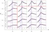 |
Fig. B.1 Amplitude of the mutual impedance spectra, simulated by Model 1, expressed in logarithmic scale as 20 log10(|Z(Ω)∕Z0|) in anti-phased SDL sub-mode (purple points) and in phased SDL sub-mode (black points) for different temperature ratios τ = Tw ∕Tc = 10, 30, 50 and 100, from left to right, and different cold electron density ratios Nc = 0.5, 0.6, 0.7, 0.8 and 0.9 from bottom to top. The Debye length of the warm electron population is fixed to λD,w = 1 m. The blue (resp. black) vertical dotted line shows the position of the cold (resp. total) electron plasma frequency. |
The RPC-MIP spectra shaped by a double resonance are located at the right and below the red borders. The parameter range for which a double resonance in the RPC-MIP spectra is visible, corresponds to high enough cold-to-total density ratios and high enough warm-to-cold electron temperature ratio. Whatever the model, at low warm-to-cold electron temperature ratio or at low cold-to-total density ratios, a single resonance or no resonance at all is visible on the spectra. At very high cold-to-total density ratio (nc ∕ne = 0.9, first row), a double resonance appears both in Model 2, and Model 3. However, in the case of Model 3, at least one of the resonances would be below the instrumental level assumed in the resonance detection algorithm. Whatever the model, the amplitude of the resonances tends to increase as the cold-to-total density ratio; therefore, the double resonance detection probability is expected to increase accordingly. This comparison between the three models of the RPC-MIP spectra shows a similar and robust instrumental feature in the same plasma parameter space neightbordhood. Finally, previous studies have shown that the best model to fit the RPC-MIP spectra is Model 3 (Wattieaux et al. 2019). Under this model, the plasma conditions that allow an unambiguous detection of the double resonance is a large enough warm-to-cold temperature ratio (Th ∕Tc > 30) and a cold-to-total density ratio in the range 0.6 < nc∕ne < 0.9.
In this study, we considered a fixed Debye length of the warm population (λD,w = 1 m). However, the plasma parameter range for which a double resonance shapes the RPC-MIP spectra also depends on the Debye length. Model 3 shows that the range of cold-to-total density ratio is reduced toward higher values (from 0.7 to 0.9) when the Debye length increases (not shown here).
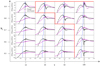 |
Fig. B.2 Same as Fig. B.1 for the RPC-MIP mutual impedance spectra modeled by the discrete-surface-charge-distribution (DSCD) without the ion sheath (Model 2). |
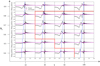 |
Fig. B.3 Same as Fig. B.1 for the RPC-MIP mutual impedance spectra modeled by the discrete-surface-charge-distribution (DSCD) considering the ion sheath around the RPC-MIP experiment (Model 3). We also added Nc = 0.4 (last row). The spectra have been normalized by the amplitude at the last frequency. |
Appendix C Detection of the main resonances on the in situ acquired RPC-MIP spectra
In this appendix, we explain how the main resonances are extracted from the acquired RPC-MIP mutual impedance spectra (i) when the spectrum is shaped by a single resonance (Fig. 2, left panel) and (ii) when the spectrum is shaped by a double resonance which indicates a mixture of cold and warm electrons in the monitored plasma (Fig. 2, right panel).
C.1 Detection of the electron plasma frequency
As explained in Sect. 2.1, the RPC-MIP measurement is based on the resonance principle of the plasma eigenmodes in the surrounding plasma. In the unmagnetized plasma of the comet 67P, only the electron plasma frequency can be detected in the frequency range of RPC-MIP. The electron plasma frequency signature is then based on the resonance frequency which corresponds,theoretically, to the maximum amplitude of a given spectrum (Chasseriaux et al. 1972; Storey 1998). However, in interplanetary plasma where the Debye length is of the order of the transmitter-receiver distance, the total plasma frequency fp is generally bounded by the maximum frequency, noted fmax and the frequency value of the spectrum minimum amplitude, noted fmin. Numerical modeling of the mutual impedance spectra shows that when the Debye length increases, the spectrum is more flattened and fmax is more and more higher than fp. For the data processing of the RPC-MIP acquired spectra, only the extremum of the spectrum as fmax can be easily retrieved. Therefore, in order to have an estimation of fp (and the total electron density ne), a calibration is based on the mutual impedance amplitude at fmax. Two main cases are then considered: (i) when the maximum amplitude is high enough, we consider that the plasma frequency is equal to fmax, (ii) when the amplitude is low, fp is located at the mean value between fmin and fmax. For instance, for the two acquired RPC-MIP spectra shown in Fig. 2, the maximum amplitude (resp. 15 dB and 20 dB) was high enough to consider fp = fmax.
C.2 Detection of the double resonance on RPC-MIP spectrum
Considering what is described previously, the detection algorithm assumes a double resonance and searches for two other extrema (a secondary minimum, noted fmin2, and a secondary maximum, noted fmax2) should be taken into account. The algorithm then sorts the retrieved extrema according to three possible configurations:
- 1.
fmin < fmax < fmin2 < fmax2
- 2.
fmin < fmax2 < fmin2 < fmax
- 3.
fmin2 < fmax2 < fmin < fmax
These three configurations are illustrated in Fig. C.1.
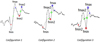 |
Fig. C.1 Three different configurations of the RPC-MIP spectrum shaped by a double resonance. The RPC-MIP spectrum is shown bythe black line and the corresponding smooth spectrum as a black dotted line. The maximum of the main resonance corresponding to the location of the maximum frequency is shown by a blue square, the minimum by a red square and the mean value by a green square. |
In order to exclude suspicious double resonances which may be generated by interferences or other artifacts, each configuration must satisfy some criteria. Following rules below are applied regarding to the given configuration. In the following, the mutual impedance amplitude obtained at frequency fi is expressed by vi.
Configuration 1 is the case where the resonance due to the cold electron population is higher than the resonance due to the total electron population (Fig. C.1, left panel). Looking for a secondary resonance, above the main resonance (fmax), implies to be sure that the amplitude difference between fmin and fmax is large enough (here 12 dB). Furthermore, the relative difference must not be too great either in frequency (|fmax2 − fmax| < 125 kHz) or in amplitude (|vmax2 − vmin2| ≥ |vmax − vmin2|∕2 > 3 dB). An amplitude range low or equal to 3 dB is considered as noise in the RPC-MIP context.
Configuration 2 is the case where the main resonance corresponds to the total electron population and where the minimum amplitude between the two resonance is higher than the global one. (Fig. C.1, middle panel). As described in the previous configuration, the relative difference in amplitude (vmax and vmax2) must not be too great. Furthermore, secondary resonances must not be confused either in frequency (|fmin2–fmax2| > 7 kHz) or in amplitude (|vmin2–vmax2| > 2 dB).
The last configuration is the case where the main resonance corresponds to the total electron population and where the global minimum is located between the two resonances (Fig. C.1, right panel). Looking for a secondary resonance, above the main resonance fmax, implies certainly that the amplitude difference between fmin and fmax is large enough (here 6 dB). Furthermore, the relative difference must not be too great either in frequency (fmin2 and frequency value of the smoothed spectrum minimum amplitude shown in dotted line) or in amplitude (|vmax2 − vmin2|≥|vmax − vmin|∕2 > 3 dB and |vmax − vmin| > 6 dB). If one of the three configurations is satisfied, we consider that a double resonance shapes the mutual impedance spectrum acquired by RPC-MIP, which corresponds to a measurement of a mixed warm and cold electrons in the surrounded plasma.
References
- Balsiger, H., Altwegg, K., Bochsler, P., et al. 2007, Space Sci. Rev., 128, 745 [NASA ADS] [CrossRef] [Google Scholar]
- Béghin, C. 1995, Rad. Sci., 30, 307 [NASA ADS] [CrossRef] [Google Scholar]
- Béghin, C., & Debrie, R. 1972, J. Plasma Phys., 8, 287 [NASA ADS] [CrossRef] [Google Scholar]
- Béghin, C., & Kolesnikova, E. 1998, Rad. Sci., 33, 503 [NASA ADS] [CrossRef] [Google Scholar]
- Béghin, C., Debrie, R., Berthelier, J. J., et al. 1982, Adv. Space Res., 2, 61 [NASA ADS] [CrossRef] [Google Scholar]
- Béghin, C., Hamelin, M., Lebreton, J. P., et al. 2017, J. Geophys. Res. Space Phys., 122, 6964 [CrossRef] [Google Scholar]
- Broiles, T. W., Burch, J. L., Chae, K., et al. 2016a, MNRAS, 462, S312 [CrossRef] [Google Scholar]
- Broiles, T. W., Livadiotis, G., Burch, J. L., et al. 2016b, J. Geophys. Res. Space Phys., 121, 7407 [Google Scholar]
- Burch, J. L., Goldstein, R., Cravens, T. E., et al. 2007, Space Sci. Rev., 128, 697 [NASA ADS] [CrossRef] [Google Scholar]
- Carr, C., Cupido, E., Lee, C. G. Y., et al. 2007, Space Sci. Rev., 128, 629 [NASA ADS] [CrossRef] [Google Scholar]
- Chasseriaux, J. M., R. Debrie, R. D., & C. Renard, C. R. 1972, J. Plasma Phys., 8, 231 [NASA ADS] [CrossRef] [Google Scholar]
- Churyumov, K. I., & Gerasimenko, S. I. 1972, IAU Symp., 45, 27 [NASA ADS] [Google Scholar]
- Clark, G., Broiles, T. W., Burch, J. L., et al. 2015, A&A, 583, A24 [NASA ADS] [CrossRef] [EDP Sciences] [Google Scholar]
- Cravens, T. E., Kozyra, J. U., Nagy, A. F., Gombosi, T. I., & Kurtz, M. 1987, J. Geophys. Res., 92, 7341 [Google Scholar]
- Deca, J., Divin, A., Henri, P., et al. 2017, Phys. Rev. Lett., 118, 205101 [NASA ADS] [CrossRef] [Google Scholar]
- Deca, J., Henri, P., Divin, A., et al. 2019, Phys. Rev. Lett., 123, 055101 [Google Scholar]
- Décréau, P. M. E., Béghin, C., & Parrot, M. 1978, Space Sci. Rev., 22, 581 [Google Scholar]
- Derfler, H., & Simonen, T. C. 1969, Phys. Fluids, 12, 269 [Google Scholar]
- Edberg, N. J. T., Eriksson, A. I., Odelstad, E., et al. 2015, Geophys. Res. Lett., 42, 4263 [NASA ADS] [CrossRef] [Google Scholar]
- Edberg, N. J. T., Eriksson, A. I., Vigren, E., et al. 2019, AJ, 158, 71 [Google Scholar]
- Engelhardt, I. A. D., Eriksson, A. I., Vigren, E., et al. 2018, A&A, 616, A51 [NASA ADS] [CrossRef] [EDP Sciences] [Google Scholar]
- Eriksson, A. I., Boström, R., Gill, R., et al. 2007, Space Sci. Rev., 128, 729 [NASA ADS] [CrossRef] [Google Scholar]
- Eriksson, A. I., Engelhardt, I. A., André, M., et al. 2017, A&A, 605, A14 [NASA ADS] [CrossRef] [EDP Sciences] [Google Scholar]
- Fried, B. D., & Conte, S. D. 1961, The Plasma Dispersion Function (New York: Academic Press) [Google Scholar]
- Galand, M., Héritier, K. L., Odelstad, E., et al. 2016, MNRAS, 462, S331 [CrossRef] [Google Scholar]
- Gary, S. P. 1993, Theory of Space Plasma Microinstabilities (Cambridge: Cambridge University Press), 193 [Google Scholar]
- Gasc, S., Altwegg, K., Balsiger, H., et al. 2017, MNRAS, 469, S108 [Google Scholar]
- Geiswiller, J., Béghin, C., Kolesnikova, E., et al. 2001, Planet. Space Sci., 49, 633 [NASA ADS] [CrossRef] [Google Scholar]
- Gilet, N., Henri, P., Wattieaux, G., Cilibrasi, M., & Béghin, C. 2017, Rad. Sci., 52, 1432, 2017RS006294 [NASA ADS] [CrossRef] [Google Scholar]
- Gilet, N., Henri, P., Wattieaux, G., et al. 2019, Front. Astron. Space Sci., 6, 16 [Google Scholar]
- Glassmeier, K.-H., Richter, I., Diedrich, A., et al. 2007, Space Sci. Rev., 128, 649 [NASA ADS] [CrossRef] [Google Scholar]
- Goetz, C., Koenders, C., Hansen, K. C., et al. 2016a, MNRAS, 462, S459 [Google Scholar]
- Goetz, C., Koenders, C., Richter, I., et al. 2016b, A&A, 588, A24 [Google Scholar]
- Grard, R. 1969, Alta Freq., 38, 97 [Google Scholar]
- Gulkis, S., Allen, M., von Allmen, P., et al. 2015, Science, 347, aaa0709 [Google Scholar]
- Hajra, R., Henri, P., Vallières, X., et al. 2018, MNRAS, 475, 4140 [NASA ADS] [CrossRef] [Google Scholar]
- Hansen, K. C., Altwegg, K., Berthelier, J.-J., et al. 2016, MNRAS, 462, S491 [Google Scholar]
- Hässig, M., Altwegg, K., Balsiger, H., et al. 2015, Science, 347, aaa0276 [Google Scholar]
- Henri, P., Vallières, X., Hajra, R., et al. 2017, MNRAS, 469, S372 [Google Scholar]
- Héritier, K. L., Henri, P., Vallières, X., et al. 2017, MNRAS, 469, S118 [CrossRef] [Google Scholar]
- Héritier, K. L., Galand, M., Henri, P., et al. 2018, A&A, 618, A77 [NASA ADS] [CrossRef] [EDP Sciences] [Google Scholar]
- Hoang, M., Altwegg, K., Balsiger, H., et al. 2017, A&A, 600, A77 [NASA ADS] [CrossRef] [EDP Sciences] [Google Scholar]
- Itikawa, Y. 2002, J. Phys. Chem. Ref. Data, 31, 749 [Google Scholar]
- Itikawa, Y., & Mason, N. 2005, J. Phys. Chem. Ref. Data, 34, 1 [NASA ADS] [CrossRef] [Google Scholar]
- Kasaba, Y., Kojima, H., Moncuquet, M., et al. 2020, Space Sci. Rev., 216, 65 [Google Scholar]
- Krall, N. A., & Trivelpiece, A. W. 1973, Principles of Plasma Physics (New York: McGraw-Hill Book Company) [Google Scholar]
- Kramer, T., Läuter, M., Rubin, M., & Altwegg, K. 2017, MNRAS, 469, S20 [CrossRef] [Google Scholar]
- Läuter, M., Kramer, T., Rubin, M., & Altwegg, K. 2019, MNRAS, 483, 852 [Google Scholar]
- Madanian, H., Cravens, T. E., Rahmati, A., et al. 2016, J. Geophys. Res. Space Phys., 121, 5815 [NASA ADS] [CrossRef] [Google Scholar]
- Mandt, K. E., Eriksson, A., Edberg, N. J. T., et al. 2016, MNRAS, 462, S9 [Google Scholar]
- Meyer-Vernet, N., Couturier, P., Hoang, S., Perche, C., & Steinberg, J. L. 1986, Geophys. Res. Lett., 13, 279 [Google Scholar]
- Myllys, M., Henri, P., Galand, M., et al. 2019, A&A, 630, A42 [NASA ADS] [CrossRef] [EDP Sciences] [Google Scholar]
- Navet, M., Bertrand, P., Feix, M., Rooy, B., & Storey, L. 1971, J. Phys. Colloq., 32, C5b [CrossRef] [Google Scholar]
- Odelstad, E., Eriksson, A. I., Edberg, N. J. T., et al. 2015, Geophys. Res. Lett., 42, 10 [CrossRef] [Google Scholar]
- Odelstad, E., Stenberg-Wieser, G., Wieser, M., et al. 2017, MNRAS, 469, S568 [Google Scholar]
- Odelstad, E., Eriksson, A. I., Johansson, F. L., et al. 2018, J. Geophys. Res. Space Phys., 123, 5870 [NASA ADS] [CrossRef] [Google Scholar]
- Sishtla, C. P., Divin, A., Deca, J., Olshevsky, V., & Markidis, S. 2019, Phys. Plasmas, 26, 102904 [Google Scholar]
- Snodgrass, C.,& Jones, G. 2019, Nat. Commun., 10, 5418 [NASA ADS] [CrossRef] [Google Scholar]
- Storey, L. R. O. 1998, Measurement Techniques in Space Plasmas: Fields (Washington DC: American Geophysical Union Geophysical Monograph Series), 103, 155 [CrossRef] [Google Scholar]
- Storey, L. R. O., Aubry, M. P., & Meyer, P. 1969, in Plasma Waves in Space and in the Laboratory, eds. J. O. Thomas, & B. J. Landmark (Edinburgh: Edinburgh University Press), 303 [Google Scholar]
- Taylor, M. G. G. T., Altobelli, N., Buratti, B. J., & Choukroun, M. 2017, Phil. Trans. R. Soc. London, Ser. A, 375, 20160262 [NASA ADS] [CrossRef] [Google Scholar]
- Trotignon, J. G., Béghin, C., Lagoutte, D., et al. 2006, Adv. Space Res., 38, 686 [Google Scholar]
- Trotignon, J. G., Michau, J. L., Lagoutte, D., et al. 2007, Space Sci. Rev., 128, 713 [NASA ADS] [CrossRef] [Google Scholar]
- Vigren, E., & Galand, M. 2013, ApJ, 772, 33 [Google Scholar]
- Vigren, E., Galand, M., Eriksson, A. I., et al. 2015, ApJ, 812, 54 [NASA ADS] [CrossRef] [Google Scholar]
- von Rosenvinge, T. T., Brandt, J. C., & Farquhar, R. W. 1986, Science, 232, 353 [CrossRef] [PubMed] [Google Scholar]
- Wattieaux, G., Gilet, N., Henri, P., Vallières, X., & Bucciantini, L. 2019, A&A, 630, A41 [NASA ADS] [CrossRef] [EDP Sciences] [Google Scholar]
- Wattieaux, G., Henri, P., Gilet, N., Vallières, X., & Deca, J. 2020, A&A, 638, A124 [NASA ADS] [CrossRef] [EDP Sciences] [Google Scholar]
- Zwickl, R. D., Baker, D. N., Bame, S. J., et al. 1986, Geophys. Res. Lett., 13, 401 [CrossRef] [Google Scholar]
All Tables
Characteristics of the RPC-MIP dataset per operational SDL sub-mode (E1, E2, anti-phased and phased) for the whole cometary phase of the mission: (i) total count of acquired mutual impedance spectra, (ii) count of the extracted electron density from RPC-MIP spectra, (iii) percentage of cold electron detections for each SDL sub-mode and (iv) distribution of the cold electron detections.
All Figures
|
Fig. 1 (a) Mutual Impedance Probe (RPC-MIP) onboard the Rosetta spacecraft consists of two transmitters (E1 and E2) and two receivers (R1 and R2) carried by a 1m-long bar (picture adapted from Trotignon et al. (2006)) and (b) RPC-MIP location at the edge of a 1.8-m boom on the Rosetta spacecraft and location of the two Langmuir probes RPC-LAP1 and RPC-LAP2 (Copyright: ESA/ATG medialab). |
| In the text | |
|
Fig. 2 Two typical in situ acquired RPC-MIP mutual impedance spectra (after compensation of instrumental effects such as interferences and solar wind response removal) in the ionosphere of 67P, from which the electron plasma frequency, fp, (shown by a vertical black line) is obtained, both in a plasma dominated by a warm electron population and characterized by a single resonance (left panel), and in a plasma characterized by a mixture of warm and cold electron populations and characterized by a double resonance (right panel). For the first (resp. second) spectrum, fp = 274 kHz (resp. fp = 421 kHz) corresponding to ne = 924 cm−3 (resp. ne = 2198 cm−3). These two spectra have been measured with the RPC-MIP phased SDL sub-mode. |
| In the text | |
|
Fig. 3 Overview of the comet escort phase. First panel: main SDL/LDL mode operated by RPC-MIP per day: the anti-phased SDL sub-mode is represented in yellow, the phased SDL sub-mode in green, and the others mode (E1,E2 and LDL mode) in grey. Second panel: daily average of the number of cold electron signatures (blue line) and the ratio between the cold electron detection and the total number of measured spectra (red line). Third panel: location of the diamagnetic cavity crossings observed by the RPC-MAG fluxgate magnetometer. Fourth panel: the cometocentric distance of Rosetta (black line) and the electron-neutral collision dominated region (exobase) (blue point) expressed in km in logarithmic scale. The surface of 67P is shown by the red line. Fifth panel: Rosetta latitude (green line) expressed in degrees and the heliocentric distance (yellow line). |
| In the text | |
|
Fig. 4 Maps of the fraction of RPC-MIP spectra showing a cold electron signature compared to the total RPC-MIP spectra acquired in phased SDL sub-mode. Left panel: 2D longitude/latitude map from 2015 Sept 4 to 2016 May 21 when the southern (resp. northern) hemisphere was in summer (resp. winter). Right panel: 2D longitude/latitude map from 2016 May 22 to 2016 Sept 30 when the southern (resp. northern) was in autumn (resp. spring). The color bar gives the cold-to acquired ratio measured by RPC-MIP from 0 to 1 (white to blue). Grey corresponds to non-detection areas. |
| In the text | |
|
Fig. 5 Histograms of the count of RPC-MIP cold electron signatures (blue bars), the count of derived RPC-MIP electron densities (red bars) and the total count of mutual impedance spectra acquired in the phased SDL sub-mode (black bars) compared to the sine of the latitude (top panels) and the longitude expressed in degrees (bottom panels). The cold-to-acquired ratio is shown in yellow squares. Left panels: from 2015 Sept. 4 to 2016 May 21 corresponding to the southern (resp. northern) hemisphere in summer (resp. winter). Right panels: from 2016 May 22 to 2016 Sept. 2016 corresponding to the southern (resp. northern) hemisphere in autumn (resp. spring). |
| In the text | |
|
Fig. 6 Histogram of the count of cold electron detections by RPC-MIP (blue bars), the count of RPC-MIP electron density measurement (red bars) and the count of mutual impedance spectra acquired in phased SDL sub-mode (black bars) as function of the heliocentric distance expressed in AU. The cold-to-acquired ratio is shown as a line of yellow squares. The line of green squares shows the fraction of time where Rosetta was in the southern hemisphere. Heliocentric distances corresponding to Rosetta nightside excursion are shaded in grey. |
| In the text | |
|
Fig. 7 Histograms of the count of cold electron detections by RPC-MIP (blue bars), the count of RPC-MIP electron density measurement (red bars) and the count of mutual impedance spectra acquired in phased SDL sub-mode (black bars) as a function of the cometocentric distance expressed in km. The cold-to-acquired ratio is shown as a line of yellow squares. The line of green squares shows the fraction of time where Rosetta was in the southern hemisphere. Each histogram ismade for a different range of heliocentric distances. |
| In the text | |
|
Fig. 8 Distance of the electron exobase Len compared to the cometocentric distance of Rosetta rs/c. The colored data shows the cold electrons detected by the double resonance on the RPC-MIP spectra and the grey data shows all acquired spectra in phased SDL sub-mode. The red line shows where rs/c = Len and the blue vertical line shows the surface of 67P defined at around 2 km. |
| In the text | |
|
Fig. 9 Count of cold electron detections by RPC-MIP (line of blue squares), count of electron density derivation (line of red squares) and count of acquired mutual impedance spectra (line of black squares) for each diamagnetic cavity crossing when RPC-MIP operated in phased SDL sub-mode. The ratio of RPC-MIP cold electron detections with the total acquired mutual impedance spectra is shown in yellow points. |
| In the text | |
|
Fig. 10 Histograms of the cold electron detections by RPC-MIP normalized by the total in situ RPC-MIP acquired spectra for the time periods where (i) the RPC-LAP observed cold electrons (first panel) and where (ii) the RPC-LAP does not observed cold electrons (second panel). All are obtained when the RPC-MIP operated in SDL phased sub-mode. The mean (yellow vertical bar) and the median (green vertical bar) of the ratio are also shown in the two histograms. |
| In the text | |
|
Fig. 11 Scatter plot of all simultaneous measurements (RPC-MIP and RPC-LAP measurements where made within 1 sec, considering only RPC-MIP phased SDL sub-mode) showing RPC-MIP total electron density, expressed in cm−3 versus the RPC-LAP I-V curve slope, expressed in nA/V. Measurements are subdivided in three cases: RPC-LAP and RPC-MIP both observed cold electrons (blue points), RPC-LAP observed cold electrons while RPC-MIP did not (green points) and RPC-MIP observed cold electrons while RPC-LAP did not (red points). The grey horizontal bars indicate the electron density corresponding to the well-known RPC-MIP interferences (see Sect. 2.2). |
| In the text | |
|
Fig. 12 First panel: map of the cold-to-acquired ratio compared to the latitude and the cometocentric distance. Second panel: map of the neutral density, expressed in cm−3, given by ROSINA-COPS compared to the latitude and the cometocentric distance. Third panel: map of the total electron density, expressed in cm−3, retrieved byRPC-MIP compared to the latitude and the cometocentric distance. The data are given from 2016 August 2 to 30. |
| In the text | |
|
Fig. A.1 Number of expected collisions (shown by the colorbar) undergone by an electron born at the nucleus surface, moving radially away from the nucleus and ballistically, before reaching the spacecraft location, depending on the outgassing rate, expressed in s−1, and the spacecraft-comet distance, expressed in km. The conditions encountered by Rosetta between 1st and 15th August 2016 are given by the black points. |
| In the text | |
|
Fig. B.1 Amplitude of the mutual impedance spectra, simulated by Model 1, expressed in logarithmic scale as 20 log10(|Z(Ω)∕Z0|) in anti-phased SDL sub-mode (purple points) and in phased SDL sub-mode (black points) for different temperature ratios τ = Tw ∕Tc = 10, 30, 50 and 100, from left to right, and different cold electron density ratios Nc = 0.5, 0.6, 0.7, 0.8 and 0.9 from bottom to top. The Debye length of the warm electron population is fixed to λD,w = 1 m. The blue (resp. black) vertical dotted line shows the position of the cold (resp. total) electron plasma frequency. |
| In the text | |
|
Fig. B.2 Same as Fig. B.1 for the RPC-MIP mutual impedance spectra modeled by the discrete-surface-charge-distribution (DSCD) without the ion sheath (Model 2). |
| In the text | |
|
Fig. B.3 Same as Fig. B.1 for the RPC-MIP mutual impedance spectra modeled by the discrete-surface-charge-distribution (DSCD) considering the ion sheath around the RPC-MIP experiment (Model 3). We also added Nc = 0.4 (last row). The spectra have been normalized by the amplitude at the last frequency. |
| In the text | |
|
Fig. C.1 Three different configurations of the RPC-MIP spectrum shaped by a double resonance. The RPC-MIP spectrum is shown bythe black line and the corresponding smooth spectrum as a black dotted line. The maximum of the main resonance corresponding to the location of the maximum frequency is shown by a blue square, the minimum by a red square and the mean value by a green square. |
| In the text | |
Current usage metrics show cumulative count of Article Views (full-text article views including HTML views, PDF and ePub downloads, according to the available data) and Abstracts Views on Vision4Press platform.
Data correspond to usage on the plateform after 2015. The current usage metrics is available 48-96 hours after online publication and is updated daily on week days.
Initial download of the metrics may take a while.