| Issue |
A&A
Volume 642, October 2020
|
|
|---|---|---|
| Article Number | A61 | |
| Number of page(s) | 17 | |
| Section | The Sun and the Heliosphere | |
| DOI | https://doi.org/10.1051/0004-6361/202038546 | |
| Published online | 07 October 2020 | |
Ubiquitous hundred-Gauss magnetic fields in solar spicules
1
Departament de Física, Universitat de les Illes Balears, 07122 Palma de Mallorca, Spain
e-mail: This email address is being protected from spambots. You need JavaScript enabled to view it.
2
Institute of Applied Computing & Community Code (IAC3), UIB, Spain
3
Department of Physics, Aberystwyth University, Ceredigion SY23 3BZ, UK
4
Abastumani Astrophysical Observatory, Mount Kanobili, 0301 Abastumani, Georgia
5
Instituto de Astrofísica de Canarias, La Laguna, Tenerife, Spain
6
Department of Mathematics, Physics and Electrical Engineering, Northumbria University, Newcastle Upon Tyne NE1 8ST, UK
Received:
1
June
2020
Accepted:
21
July
2020
Abstract
Aims. We aim to study the magnetic field in solar spicules using high-resolution spectropolarimetric observations in the Ca II 8542 Å line obtained with the Swedish 1-m Solar Telescope.
Methods. The equations that result from the application of the weak field approximation (WFA) to the radiative transfer equations were used to infer the line-of-sight (LOS) component of the magnetic field (BLOS). Two restrictive conditions were imposed on the Stokes I and V profiles at each pixel before they could be used in a Bayesian inversion to compute its BLOS.
Results. The LOS magnetic field component was inferred in six data sets totalling 448 spectral scans in the Ca II 8542 Å line and containing both active region and quiet Sun areas, with values of hundreds of Gauss being abundantly inferred. There seems to be no difference, from a statistical point of view, between the magnetic field strength of spicules in the quiet Sun or near an active region. On the other hand, the BLOS distributions present smaller values on the disc than off-limb, a fact that can be explained by the effect of superposition on the chromosphere of on-disc structures. We show that on-disc pixels in which the BLOS is determined are possibly associated with spicular structures because these pixels are co-spatial with the magnetic field concentrations at the network boundaries and the sign of their BLOS agrees with that of the underlying photosphere. We find that spicules in the vicinity of a sunspot have a magnetic field polarity (i.e. north or south) equal to that of the sunspot. This paper also contains an analysis of the effect of off-limb overlapping structures on the observed Stokes I and V parameters and the BLOS obtained from the WFA. It is found that this value is equal to or smaller than the largest LOS magnetic field components of the two structures. In addition, using random BLOS, Doppler velocities, and line intensities of these two structures leads in ≃50% of the cases to Stokes I and V parameters that are unsuitable to be used with the WFA.
Conclusions. Our results present a scarcity of LOS magnetic field components smaller than some 50 G, which must not be taken as evidence against the existence of these magnetic field strengths in spicules. This fact possibly arises as the consequence of signal superposition and noise in the data. We also suggest that the failure of previous works to infer the strong magnetic fields in spicules detected here is their coarser spatial and/or temporal resolution.
Key words: Sun: chromosphere / Sun: magnetic fields
© ESO 2020
1. Introduction
Spicules are cold, dense, short-lived, jet-like structures that shoot out from the chromosphere and reach coronal heights. Ever since their discovery by Secchi (1877), they have remained a topic of great interest in solar physics and nowadays it is believed that they could play an important role mediating energy and mass transport to the corona (Beckers 1968; De Pontieu et al. 2011). The term “spicule” was first coined by Beckers (1968), referring to objects visible off-limb, although they are present everywhere on the Sun and are ejected from the chromospheric network. Numerous reviews have been written as the knowledge on spicules has evolved (Beckers 1968; Sterling 2000; Rutten 2012; Tsiropoula et al. 2012; Hinode Review Team 2019).
With the advance in instrumentation, more has been learnt about spicules. Of special importance was the introduction of the Hinode satellite (Kosugi et al. 2007; Suematsu et al. 2008), which provides high-cadence, high-resolution images necessary to properly resolve small structures. Perhaps the most important discovery about spicules in recent years is that they seem to come in two types (De Pontieu et al. 2007; Pereira et al. 2012). Type I spicules are present mainly near active regions (ARs), show a rise and fall motion with constant acceleration, and are visible in chromospheric lines during their whole lifetime (Rouppe van der Voort et al. 2007; De Pontieu et al. 2007). They are longer lived and possess smaller mass flow velocities than their more energetic type II siblings, which are present everywhere on the Sun and are much more abundant. Type II spicules seem to be accelerated upwards and heated at the same time, hence they are observed at progressively hotter temperature lines, starting at chromospheric ones and then followed by transition region and coronal lines (Rouppe van der Voort et al. 2009; De Pontieu et al. 2007, 2017; Pereira et al. 2014; Henriques et al. 2016; Bose et al. 2019; Yurchyshyn et al. 2020).
Direct magnetic field measurements of spicules are very scarce and have been done by using spectropolarimetric observations coupled with a theoretical modelling of the Zeeman and Hanle effects (see Tsiropoula et al. 2012 for a review, and Socas-Navarro & Elmore 2005 and Centeno et al. 2010 for a discussion of the magnetic field determination from spectropolarimetric data). In all works, which are described next, a spectrograph slit placed on off-limb spicules was used to acquire the data. Trujillo Bueno et al. (2005) used spectropolarimetric observations in the He I 10830 Å triplet obtained with the Tenerife Infrared Polarimeter (TIP; Martínez Pillet et al. 1999; Collados et al. 2007) at the German Vacuum Tower Telescope (VTT) in the Observatorio del Teide, with a net integration time of 209 s; this time corresponds to the averaging of 50 consecutive exposures. These authors performed both optically thin and optically thick theoretical modellings of the Hanle and Zeeman effects to infer magnetic field values of 10 G in a quiet Sun (QS) region. López Ariste & Casini (2005) made spectropolarimetric observations in the He I D3 line taken with the Advanced Stokes Polarimeter (ASP; Elmore et al. 1992) at the Dunn Solar Telescope (DST) with the slit crossing an active region plage. The data have 6 s per exposure and a pixel scale of 0.29″ pixel−1, although the seeing-induced image degradation yields a much worse spatial resolution (see Fig. 6 of López Ariste & Casini 2005). These authors reported the possibility of magnetic fields stronger than 30 G, even up to 40 G. Ramelli et al. (2005, 2006) used a set of observations in the He I D3 line taken with the Zurich Imaging Polarimeter (ZIMPOL; Gandorfer et al. 2004) at the 45 cm Gregory-Coudé Telescope (GCT) at the Istituto Ricerche Solari Locarno (IRSOL) with a 2-min cadence. They created a database of theoretical Stokes profiles using the quantum theory of the Hanle and Zeeman effects, and upon inverting the observed spectropolarimetric signals, they inferred magnetic field values of 50 G near an active region and 10 G in a quiet Sun area. Centeno et al. (2010) also used observations in the He I 10830 Å triplet at the VTT with a time cadence and pixel scale of 56 s and 0.17″ pixel−1, respectively; to increase the signal-to-noise ratio (S/N), the data were spatially and temporally averaged to 1″and 45 min. Using the HAZEL code (Asensio Ramos et al. 2008) for the inversion, they could set a lower value of the magnetic field strength as high as 50 G in a quiet Sun region, namely the solar south pole. Further work on the spicules’ magnetic field was carried out by Orozco Suárez et al. (2015) with the help of spectropolarimetric He I 10830 Å data taken with the Tenerife Infrared Polarimeter II (TIP-II Collados et al. 2007) at the VTT. The exposure time was about 10 s for a fixed slit position and the spatial resolution was estimated to be in the range 0.7–1″. A 9″ wide area above the limb was scanned with the spectrograph slit, which allowed Orozco Suárez et al. (2015) to infer the magnetic field vector with the HAZEL code and to study its variation with height. These authors concluded that the magnetic field is essentially vertical at the base of the chromosphere and changes its inclination to some 40° from the vertical direction at 2 Mm height. At the same time, its strength varies from 80 G to 30 G, on average, from the base of the chromosphere to a height of 3 Mm.
Spicules are formed along chromospheric magnetic flux concentrations, therefore estimating their magnetic field is necessary in order to properly comprehend how such structures are formed and evolve. In this paper we analyse high-resolution imaging spectropolarimetric observations of solar spicules in the Ca II 8542 Å line, presented in Sect. 2. We use the Weak Field Approximation (WFA; Sect. 3), which is a computationally inexpensive method to calculate the magnetic field vector from the Stokes parameters when some conditions are met (see e.g. Landi Degl’Innocenti & Landolfi 2004; Jennerholm Hammar 2014; de la Cruz Rodríguez & van Noort 2017; Centeno 2018). This technique has been used in the past with Ca II 8542 Å observations to infer the line-of-sight (LOS) magnetic field component (BLOS) in a quiet Sun region near a decaying active region (Pietarila et al. 2007), an active region filament (Harvey 2012), flares (Harvey 2012; Kuridze et al. 2018), a sunspot umbra (de la Cruz Rodríguez et al. 2013), and flare coronal loops (Kuridze et al. 2019). Our spectropolarimetric data contain Stokes I and V profiles above the noise level, which allows us to determine the LOS magnetic field component (Sect. 4). The computed BLOS values are of the order of hundreds of G, which is substantially higher than previous estimates for solar spicules. In the discussion, Sect. 5, we use a simple model to assess the effect on the Stokes I and V parameters of two structures overlapping along the LOS and the BLOS derived from the WFA. Furthermore, we show that the measured LOS magnetic fields correspond to spicules and, by temporally averaging our data, we show that low-resolution or low-cadence spectropolarimetry can highly underestimate the magnetic field strength. Finally, Sect. 6 provides the concluding remarks.
2. Observations
The observations used in this work were obtained with the CRisp Imaging SpectroPolarimeter (CRISP; Scharmer et al. 2008) at the Swedish 1-m Solar Telescope (SST; Scharmer et al. 2003) on 02, 03, and 09 June 2016 (see Table 1 for a summary). The data sets consist of imaging spectropolarimetry in the Ca II 8542 Å line with a pixel scale of 0.057″ pixel−1. The spectral resolution is 0.05 Å at line centre and 0.25 Å at the wings, with a total of either 15 or 21 spectral positions, depending on the data set (see Table 1). Data were reconstructed with the Multi-Object Multi-Frame Blind Deconvolution (MOMFBD; Van Noort et al. 2005). The CRISP data reduction pipeline (de la Cruz Rodríguez et al. 2015) was used for additional data reduction, including the cross-correlation method of Henriques (2012). We applied no stray-light correction to our data. To test the influence of stray light on our results, we followed the procedure provided to us by Rouppe van der Voort (priv. comm.) and applied the stray-light correction to the off-limb pixels of data sets 2, 6, and 8. After repeating the analysis described in Sect. 3 we obtained results that differ by less than 1 G, which is a negligible amount.
Summary of the observational data sets.
The main targets of the different observations were active regions, or their surroundings, near the solar limb. The data sets thus contain spectropolarimetric observations of both on-disc and off-limb chromospheric structures, both in quiet Sun and in active regions. Two active regions were under study throughout the three observational days referenced here. On 02 June 2016, NOAA AR 12551 was approaching the west solar limb, finishing its transition on 03 June 2016. It was the subject of study on both observational days, enabling a comprehensive study of the magnetic topology of spicules both near and away from sunspots. On 09 June 2016, AR 12553 was observed as it was emerging from the east solar limb. In all data sets, off-limb spicules are near an active region, while on-disc spicules are in a quiet Sun region. The only exception is the data set from 02 June 2016, in which off-limb and on-disc spicules are respectively in the quiet Sun and near an active region. The disc region of this data set is dominated by a sunspot and, given that our aim is to study the magnetic field of spicules, we ignore the on-disc pixels of 02 June 2016.
Figure 1 contextualises the observations, with an image from 03 June 2016. It is compared to a simultaneous image taken with NASA’s Solar Dynamics Observatory (SDO) in the Atmospheric Imaging Assembly (AIA; Lemen et al. 2012) 171 Å channel. Figure 2 shows the four Stokes parameters from one of the 03 June 2016 data sets. The spectropolarimetric data reveal a strong circular polarisation (Stokes V) signal, specially off-limb, where there is less signal superposition. The linear polarisation (Stokes Q and U) is weaker and these data are very noisy.
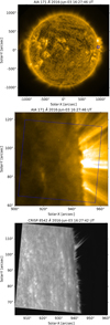 |
Fig. 1. Context of the observations of 03 June 2016 at 16:27 UT. The top panel shows the CRISP field of view (blue square) on an SDO/AIA image in the 171 Å filter. The middle panel shows a zoomed view of the top panel. The bottom panel shows a nearly co-temporal SST/CRISP image in the line centre of the Ca II 8542 Å line. Time is shown at the top of each frame and solar north is to the top. |
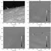 |
Fig. 2. Stokes parameters at line centre on 03 June 2016 at 16:27:42 UT. The parameters are normalised to the continuum intensity, Ic, measured as the average of I on the disc at the line wings (|Δλ| > 1.25 Å). Solar north is to the left. |
To make a quick reference to the data sets, we label each of them with a number. Since we analysed separately on-disc and off-limb pixels, each data set was split into two, so that a different number is assigned in Table 1 to off-limb and on-disc data. Adding all data sets, we have 448 spectropolarimetric scans in the Ca II 8542 Å line, each of them containing some 1000 × 1000 pixels.
3. Data analysis
In this section we describe the procedure used to infer the BLOS component from the Stokes I and V in every pixel of each scan.
3.1. Weak-Field Approximation (WFA)
In order to infer the LOS magnetic field component, BLOS, the Weak Field Approximation (WFA; Landi Degl’Innocenti & Landolfi 2004; Centeno 2018; Kuridze et al. 2019) was used. The WFA is a simplification of the radiative transfer equations as a function of the Stokes parameters that can be applied when some conditions are met.
The first condition is that the Zeeman width (ΔλB) needs to be much smaller than the Doppler width (ΔλD),
 (1)
(1)
where  is the effective Landé factor of the line (Landi Degl’Innocenti 1982), which for the Ca II 8542 Å line is 1.1. The above inequality can be written as
 (2)
(2)
where T is the temperature (in Kelvin), λ0 is the wavelength of the transition (in Å), μ is the atomic weight of the species, ξ is the microturbulent velocity (in km s−1), and B is the magnetic field intensity (in Gauss). The second condition is that the BLOS component must be uniform in the regions of line formation along the LOS. Following the derivation presented by Landi Degl’Innocenti & Landolfi (2004), a perturbative scheme can be applied to the radiative transfer equations when such conditions are met and a relation between the Stokes I and V parameters can be derived:
 (3)
(3)
where f is the magnetic filling factor (Landi Degl’Innocenti & Landolfi 2004; Asensio Ramos 2011), which here is assumed to be unity at chromospheric heights due to the expansion of the magnetic field. As pointed out by Centeno (2018), however, f = 1 might not be true everywhere in the Sun (Sainz Dalda & López Ariste 2007) and one must keep this in mind when analysing the results presented here. After properly assessing the applicability of the theory, the LOS magnetic field component can be inferred from the observed Stokes profiles with Eq. (3).
3.2. Weak Field Approximation conditions
In order to properly make use of the WFA and to ensure its validity, two restrictions on the Stokes I and V profiles were imposed on every pixel of each data set. If one of the restrictions was not met, the pixel was not used in the analysis and its BLOS was not calculated. The first condition comes directly from Eq. (2). Substituting the numerical values for the Ca II 8542 Å line, a temperature of 7500 K and a microturbulent velocity1 of 3 km s−1 results in the condition
 (4)
(4)
In principle, magnetic fields of such intensity are not expected to be present at chromospheric heights outside sunspots.
We now analyse the requirement that the LOS magnetic field component must be independent of optical depth. The presence of a magnetic field gradient along the LOS can leave footprints on the profiles of the circularly polarised radiation (Sigwarth 2001; Sheminova 2005; Solanki 1993). In a static atmosphere the usual profile of the Stokes V parameter as a function of wavelength is characterised by two lobes of equal area and amplitude, with a zero crossing at the line centre, λ0 (Auer & Heasley 1978). A typical asymmetric Stokes V profile is shown in Fig. 3, in which several parameters used to quantify the Stokes V asymmetry are defined. Amplitude and area asymmetries of the circularly polarised radiation, V, are strongly linked to variations in the magnetic field configuration combined with velocity shifts along the LOS. Furthermore, velocity gradients along the LOS also give rise to asymmetries in Stokes I (Kuridze et al. 2015). This means that they also produce area and amplitude asymmetries in the Stokes V lobes. Then, very asymmetric circular polarisation signals must be filtered out. The presence of noise in the data can also give rise to Stokes V asymmetries, which further complicates the analysis. Hence, a careful assessment of the asymmetry of the observed profiles must be devised before applying Eq. (3).
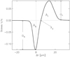 |
Fig. 3. Typical asymmetric Stokes V profile (from Sheminova 2005). The meaning of the various quantities is given in the text. |
The definitions of area and amplitude asymmetries used here are, respectively,
 (5)
(5)
and
 (6)
(6)
where Ab and Ar are the respective areas of the Stokes V blue and red lobes, whereas ab and ar are the respective amplitudes of the Stokes V blue and red lobes (see Fig. 3).
In order to control the asymmetry of the Stokes V profile, the following condition was imposed:
 (7)
(7)
Here ε is a number between 0 and 1 (we took2ε = 0.5) and η is the average amplitude of the noise present in the specific time instant of the data set under consideration. It was estimated by averaging the signal far off-limb where only noise is expected to be present. In our analysis we saw that almost every time that condition (7) was met, the area asymmetry was smaller than the amplitude asymmetry. Hence, no restriction was imposed on δA.
3.3. Method
In this work we used a Bayesian approach to infer parameters at each pixel and each time, but before applying this technique we had to ensure that the Stokes I and V profiles were suitable for the WFA. Emission (absorption) Stokes I profiles that possess more than one maximum (more than one minimum) were not analysed because they may arise from the superposition along the LOS of two structures with different Doppler velocities. After this, the first step was based on the fact that Eq. (3) establishes a linear relation between V(λ) and ∂I/∂λ. The Pearson correlation coefficient (Pearson & Galton 1895), R, between such quantities was calculated in every pixel, and only those for which |R| > 0.9 were selected. Figure 4 shows a comparison between a profile that meets such criterion and a profile that does not, evidencing the need to impose this constraint on R.
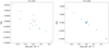 |
Fig. 4. Stokes V against ∂I/∂λ for a pixel in which |R| < 0.9 (left) and a pixel in which |R| > 0.9. The corresponding values of R are shown on top of each panel. |
After pixels for which the correlation criterion did not hold were filtered out, the next step was to analyse the asymmetry of the Stokes V profile. Condition (7) requires a precise measurement of ab and ar. This is troublesome when dealing with our data sets, since only 15 or 21 spectral positions are sampled, so that the actual extrema of V will most likely not fall exactly at one of the sampled wavelengths. For this reason, and also because our measurements are affected by noise, two models were fitted to the observed profiles in order to determine their asymmetry more accurately. The first model is a simple sum of Gaussian functions, with six free parameters, while the second model is the derivative of a skewed Gaussian function, with four free parameters to adjust. Both models allow for the existence of asymmetries. The Bayesian information criterion (BIC; Schwarz 1978) was used to identify the model that best fits the Stokes V profile at each pixel3. The value of δa was established from the fitted profile and condition (7) was checked. An example of a V(λ) profile that does not meet the asymmetry criterion is shown in the left panel of Fig. 5 alongside one that does meet such a criterion in the right panel.
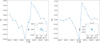 |
Fig. 5. Examples of Stokes V profiles in which the correlation criterion |R| > 0.9 is met. Left: the asymmetry criterion is not satisfied. Right: the asymmetry criterion is satisfied. The insets show the plots of Stokes V vs. ∂I/∂λ, both of which have passed the filter |R| > 0.9. |
After imposing the correlation and asymmetry criteria to all pixels, we were left with those whose Stokes I and V profiles are suitable for the application of the WFA. We used Bayes’ formula
 (8)
(8)
where P(params|data) is the posterior distribution, which once obtained gives the probability distribution of the parameters given the observed data (i.e. I and V); P(params) is the prior distribution, which reflects the belief one has about the values that the unknown parameters can take before the measurements are performed; and P(data|params) is the likelihood distribution, which gives the probability distribution of possible values of V(λ) and ∂I/∂λ that can be measured for given values of the parameters. In the absence of noise and for a fixed BLOS, V(λ) would be given by the right-hand side of Eq. (3). The presence of noise in the data, however, affects this measurement and for this reason the likelihood distribution was chosen as a Gaussian distribution for V(λ) centred at the value given by the right-hand side of Eq. (3) and with a standard deviation σ. This means that, besides BLOS, there is a second unknown parameter, σ. Regarding the prior distribution, the choice made here was to assign a uniform prior to BLOS centred at the value obtained from the slope, s, of the least-squares fit of V(λ) versus ∂I/∂λ:
 (9)
(9)
and with a width of 500 G. We tried other values of the width and found that this one is suitable: it does not constrain the Bayesian inference too much so as to force it to yield a BLOS in a narrow range, such as would happen for a much smaller width, and does not carry with it the penalty of a higher computation time, such as would be the case for a larger width. A half-Cauchy distribution was chosen as a prior for σ, fixing the scale parameter β to 0.5, so that the distribution has mode 0 and σ has a 70% probability of being less than one. The values β = 1 and β = 2 were used in preliminary tests, yielding identical results but with longer computational time.
In order to carry out the product between the likelihood and the prior distributions, and to obtain the posterior distribution and the marginalisation, a numerical sampler is needed. This was done with PyMC3 (Salvatier et al. 2016), a Python package devoted mainly to Bayesian inference problems. PyMC3 makes use of Markov chain Monte Carlo methods to sample the posterior, and it also includes a wide functionality for summarising model statistics and the output. We finally got the posterior distribution for BLOS and σ. One particular statistic of interest of these probability distributions is the highest posterior density (HPD) interval. A 100 (1 − α)% HPD interval is a region that satisfies the following two conditions:
-
the posterior probability of that region is 100(1 − α)%;
-
the minimum density of any value within that region is equal to or larger than the density of any point outside that region.
An example of the resulting posterior distributions for one pixel is shown in Fig. 6. In order to summarise the posterior distribution of each pixel, the mode of BLOS will be given as its representative value, combined with the 95% HPD interval as a measure of the most probable values of BLOS.
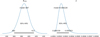 |
Fig. 6. Results of the Bayesian inference for one pixel. The mode of the posterior distribution and the 95% HPD interval of BLOS (left; in Gauss) and σ (right; in normalised count units) are shown. |
4. Results
In this section we present the results of the Bayesian inference. The association of the measured LOS magnetic field components with spicules is done in Sect. 5.2.
4.1. Off-limb pixels
The method described in Sect. 3 was applied to all pixels located above the limb in each data set, where the limb is defined as the sharp intensity transition in the wings of the Stokes I profile. The top panel of Fig. 7 shows spicules from data set 1 with the points that passed the correlation and asymmetry criteria for a particular time instant plotted on the corresponding intensity image. The majority of these points are located between 2″ and 5″ (1450 and 3625 km) above the limb, the reason being that both the pixels at heights smaller than 2 Mm, in which superposition becomes too strong for the WFA to be applicable (see Sect. 5.1), and the pixels of faint spicular material at larger heights fail to meet the two criteria.
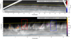 |
Fig. 7. Results from the Bayesian inference for the off-limb data of 02 June 2016 at 07:46:06 UT, belonging to data set 1 (top frame), and 03 June 2016 at 16:43:20 UT, belonging to data set 8 (bottom frame). The points are coloured based on the mode from the posterior distribution of the LOS magnetic field intensity (see colour bar at the right) and are plotted on top of the Ca II 8542 Å line centre intensity image. The blue line represents the position of the solar limb, while the black and yellow curves represent the heights 2″ and 5″ above the limb, respectively. The red and blue rectangles in the bottom panel are used in Fig. 14. |
We note that data set 1 is the only one that contains off-limb spicules far from an active region. The lack of a predominant north or south magnetic polarity in the set of spicules coupled with their wide range of inclinations allows for both positive and negative BLOS, as evidenced by the values in the colour bar of Fig. 7, top. In addition, this figure also indicates that, although not many pixels pass our two selection criteria, |BLOS| values well in excess of 100 G prevail. In Fig. 8 all the inferred values of BLOS for each of the off-limb data sets listed in Table 1 are put together by means of a histogram. The top left panel, corresponding to data set 1, reveals that the number of pixels for which the LOS magnetic field could be determined is considerable and that |BLOS| reaches values as high as 800 G. A summary of the results of Fig. 8 is shown in Table 2, in which the mode and the 95% HPD interval of the distributions shown in Fig. 8 are computed, using the absolute value of BLOS.
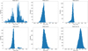 |
Fig. 8. Histogram of BLOS values for the off-limb pixels. The data set labels are those given in Table 1. |
Off-limb pixels.
Next we present the results of data set 8, an example of an active region area with off-limb spicules. The bottom panel of Fig. 7 is analogous to the top one in that LOS magnetic field components greater than 100 G are abundant in the region between 2″ and 5″ above the limb and that WFA inversions are absent outside this area. The main differences between the two figures are that it was possible to carry out the Bayesian inversion for many more pixels and that all measured BLOS are positive. This is also true for the whole duration of this data set, as shown by the histogram in Fig. 8 (second row, centre). This result is very robust because the number of pixels of data set 8 for which the BLOS has been computed is about an order of magnitude larger than that of data set 1. Hence, we have found strong evidence of magnetic fields that point towards the observer whose LOS components are clustered around 200 G; in particular, the mode of their distribution is 193 G (see Table 2). But what is the reason for this particular orientation of the magnetic field vectors in the whole area? To explain this we make use of Fig. 9, where a sketch of the region observed in data sets 2, 4, 6, and 8 is shown. NOAA AR 12551 had a leading south magnetic polarity and a trailing north magnetic polarity that at the observing time of data set 8 were both on the non-visible side of the west limb. Assuming that the magnetic field of spicules in the close vicinity of each active region magnetic polarity is not randomly oriented but has the same orientation of this polarity (such as hypothesised by Orozco Suárez et al. 2015), all spicules visible in data set 8 possess a magnetic field pointing towards the observer, except for a tiny number of pixels with negative BLOS around −100 G (see Fig. 8, second row, centre), which do not follow this orientation pattern.
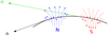 |
Fig. 9. Schematic representation of the magnetic polarity of AR 12551 and the spicule fields (short blue and red arrows) around the dominant magnetic polarities (long blue and red arrows). The green and black straight lines respectively represent the line-of-sight tangent to the solar limb of data sets 2, 4, and 6 (morning of 03 June 2016), and of data set 8 (afternoon of 03 June 2016). |
Now we turn our attention to data sets 2, 4, and 6, which were acquired a few hours before data set 8 over a time span of 90 min. The green line of Fig. 9 suggests that at the time when these three data sets were taken, the off-limb LOS intersected both a north polarity and a south polarity spicule area with the magnetic field pointing away from the observer, hence the negative sign of BLOS in the histograms of Fig. 8. Once more, |BLOS| is greater than 200 G for a considerable number of pixels (see Table 2 for the |BLOS| mode of each data set) and a minority of pixels with a polarity opposite to the prevailing one are also present.
Data set 10 was acquired above an active region on the east limb. Figure 8 (bottom right panel) demonstrates that this is the case in which we find the highest number of pixels that have passed the filters for the computation of BLOS. The spicules in this data set were near the north magnetic polarity of the active region which, at the observing time, had not yet reached the limb. Therefore, the magnetic field in the spicules pointed towards the observer and positive BLOS are obtained. This result reinforces our previous hypothesis of a dominant spicule polarity in the areas adjacent to the dominant active region polarities. In this case, the BLOS cluster around a much higher value than for data sets 2, 4, 6, and 8, namely around 450 G (Table 2).
In this section we have presented the results for off-limb pixels and, in order to explain the prevailing positive or negative signs of the inferred BLOS in all data sets except 1, have put forward the hypothesis that this is the consequence of spicules near a sunspot having the magnetic polarity of that sunspot. In Sect. 5.2 we provide evidence that the pixels for which the application of the WFA has given a BLOS value actually belong to spicules. Furthermore, an inspection of the distributions of Fig. 8 shows that the largest BLOS values correspond to both quiet Sun spicules (data set 1) and spicules near an active region (data set 10). Hence, there seems to be no difference in the magnetic field strength of spicules in the quiet Sun and near an active region. Moreover, we mentioned before that the number of pixels for which BLOS could determined is much smaller for data set 1 than for the other data sets. Although this might be caused by the worse seeing of data set 1, we offer another explanation. The superposition along the LOS of different structures may lead to observed Stokes I and V that do not pass the imposed criteria before the WFA is applied (see Sect. 5.1). If the magnetic field orientation of spicules near an active region is more constrained than that of their quiet Sun counterparts, as we have suggested above, then quiet Sun pixels have a higher probability of containing overlapping spicules with both positive and negative BLOS, which will result in a smaller number of pixels for which BLOS can be obtained.
4.2. On-disc pixels
The same analysis was done for the pixels seen on the solar disc, which are not in the vicinity of an active region and hence are not expected to possess a predominant north or south magnetic polarity. Signal superposition (see Sect. 5.1) strongly limits the number of pixels that satisfy the correlation and asymmetry conditions. This can be seen in Fig. 10, where similar histograms to those of Fig. 8 are shown for the data sets that correspond to disc pixels. As predicted for quiet Sun pixels, both signs of BLOS are inferred. Table 3 provides a summary of the results for the on-disc spicules in a similar manner as Table 2. Based on the results of Sect. 5.1, we suggest that smaller BLOS values are obtained on the disc because of the stronger influence of superposition of the absorbing plasma elements on top of the chromosphere.
On-disc pixels.
4.3. Chromospheric anemone
The structure near coordinates (10″, 35″) of Fig. 2 is a chromospheric anemone (Shibata et al. 2007). It is a type of chromospheric jet that possesses an inverted Y-shape structure (see Fig. 11) attributed to magnetic reconnection. Even though this work is focused on spicules, the WFA can also be applied to this structure, as shown in Fig. 12. The isolation and higher Ca II 8542 Å line intensity of the anemone provide clearer I and V signals, something difficult to obtain in the lower lying spicules, which frequently overlap on top of each other. A comparison between Figs. 7 and 12 shows that the line-of-sight magnetic field component in the anemone and the neighbouring spicules has similar values. There is also an apparent tendency of BLOS to decrease with height along the anemone, an issue that will be discussed in Sect. 5.3. The distribution of BLOS in the anemone is analogous to that shown in Fig. 8. The mode of the distribution is 210 G and its 95% HPD interval is [111, 293] G.
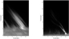 |
Fig. 11. Chromospheric anemone observed on 03 June 2016 at 16:31:50 UT, viewed in the Ca II 8542 Å line centre (left) and −0.75 Å from line centre (right). |
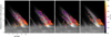 |
Fig. 12. Temporal evolution of the chromospheric anemone seen in Fig. 11 and the inferred BLOS values. The leftmost picture was taken on 03 June 2016 at 16:31:50 UT and the subsequent figures show the evolution of the region and the inferred BLOS at time intervals of 36.33 s. |
5. Discussion
This section is devoted to discuss some issues associated with the interpretation of the obtained results.
5.1. Signal superposition and integration time
We now study the effect that structures above the limb overlapping on the same detector pixel have on the BLOS obtained from the WFA. The plan is to specify the Stokes parameters of two such structures that lie along the same LOS, construct from them the observed Stokes parameters, and use Eq. (3) to calculate BLOS. For this task we used the toy model of Centeno et al. (2010), made of two slabs illuminated from below and whose radiation is detected by an observer (see their Fig. 4). The radiation emitted by slab 1, the one furthest from the observer, must cross slab 2 before reaching the detector. Centeno et al. (2010) model this effect by a wavelength-independent optical depth, τ2. We considered an optically thin plasma and hence used τ2 ≪ 1. The expressions for the detected I and V profiles, namely Eqs. (2) and (3) of Centeno et al. (2010), reduce to
 (10)
(10)
 (11)
(11)
where Ii, Vi (i = 1, 2) are the Stokes I and V emitted by the slabs. In the case of slab 2 being optically thick, Vobs ≃ V2 and Iobs ≃ I2, and therefore the measurements of BLOS will be dominated by the magnetic field of slab 2.
To construct the observed Stokes parameters with Eqs. (10) and (11) we must specify the I and V of the two slabs. Their intensity profiles were chosen as Gaussians,
![Mathematical equation: $$ \begin{aligned} I_1 = I_{01}\exp \left[-\frac{(\lambda -\lambda _\mathrm{c1} )^2}{\sigma _\mathrm{I} ^2}\right], I_2 = I_{02}\exp \left[-\frac{(\lambda -\lambda _\mathrm{c2} )^2}{\sigma _\mathrm{I} ^2}\right], \end{aligned} $$](/articles/aa/full_html/2020/10/aa38546-20/aa38546-20-eq13.gif) (12)
(12)
where we set σI = 0.5 Å, which is the typical width of the off-limb intensity profiles in our data sets. Moreover, λci, i = 1, 2, is the Doppler shifted line centre wavelength, that is, λci = λ0(1 + vDi/c) with λ0 = 8542.1 Å, and vDi is the LOS velocity of slab i. Equation (3), with f = 1, was used to calculate V1, 2 from I1, 2 given the LOS magnetic field components in the two slabs, BLOS1, 2.
Now, the Stokes profiles of each slab are characterised by the parameters I0i, vDi, and BLOSi, which makes a total of six parameters. We recall that when the LOS component of B points towards (away from) the observer, then BLOS is positive (negative). One of the intensity amplitudes, I01 and I02, can be set to an arbitrary value and the results do not change as long as the ratio I02/I01 is not altered. We thus chose I01 = 1 and left I02/I01 free. In addition, the BLOS derived from the WFA inversion of Iobs and Vobs remains almost unchanged when the Doppler velocities are varied in such a way that the difference vD2 − vD1 is kept constant. Our problem then contains four free parameters: BLOS1, BLOS2, I02/I01, and ΔvD ≡ vD2 − vD1. Once they are fixed, the Stokes I and V of each slab can be determined with Eqs. (12) and (3) and their superposition can be derived from Eqs. (10) and (11). The final step is to fit a straight line to Vobs versus ∂Iobs/∂λ and to use Eq. (9) to compute the resulting BLOS. To accept the result of this fit we imposed the restriction |R| > 0.9, where R is the Pearson correlation coefficient.
The results presented here were computed with a set of 15 wavelengths uniformly distributed in the range [λ0 − 1.5 Å, λ0 + 1.5 Å]. Using the non-uniformly spaced wavelengths of our data sets does not substantially modify the results. When both Doppler shifts are equal (ΔvD = 0) and for equal intensity amplitudes in both slabs (I02/I01 = 1), but for any value of BLOSi, we found that the BLOS given by the WFA is equal to the average of the LOS magnetic field components of the slabs, (BLOS1 + BLOS2)/2, with a correlation coefficient |R| = 1. To describe the effect of signal superposition for ΔvD ≠ 0 and/or I02/I01 ≠ 1, we considered the specific values BLOS1 = 200 G and BLOS2 = −40 G. The top panel of Fig. 13 presents the obtained BLOS as a function of ΔvD and I02/I01. To allow a comparison with the maximum LOS magnetic field component present in both slabs, the BLOS returned by the WFA is normalised to the maximum of |BLOS1|,|BLOS2|. In addition, the dashed black lines indicate the parameter values for which the condition |R| > 0.9 is met. Thus, the top panel of Fig. 13 shows that the BLOS from the WFA inversion is between 20% (red curve) and 67% (left and right ends of black line superimposed on blue curve) the maximum BLOS in the two slabs. These limits vary for other choices of BLOS1 and BLOS2 but the upper one is always smaller than or equal to 100% and only when BLOS1 ≃ BLOS2 does it approach 100% (from below). Hence, we conclude that the application of the WFA to the Stokes signals from two overlapping structures leads to a reduction of the largest BLOS present in both of them.
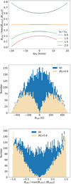 |
Fig. 13. Results of the WFA BLOS inversion when the Stokes I and V parameters in a pixel come from two overlapping structures (cf. Eqs. (10) and (11)). Top: BLOS normalised by dividing it by the maximum LOS magnetic field of the two structures, in absolute value. It is plotted vs. the difference between the two slabs’ Doppler velocity, ΔvD, for several intensity amplitude ratios, I02/I01. The dashed black lines give the results for which |R| > 0.9. In this plot BLOS1 = 200 G and BLOS2 = −40 G. Middle: BLOS distribution from the Monte Carlo experiment. Bottom: BLOS distribution divided by the maximum of |BLOS1|,|BLOS2|. In the middle and bottom panels, the blue and beige colours respectively correspond to all the samples in the Monte Carlo experiment and only those that pass the filter |R| > 0.9. |
All curves in the top panel of Fig. 13 show that large Doppler velocity differences between the two slabs spoil the WFA inversion. These curves are symmetric about ΔvD = 0, as expected. The largest values of |ΔvD| for which the WFA works are found for the blue curve, which is the one for which the slab with the largest BLOS also has the largest I amplitude (slab 1 in this example). The blue curve also gives the largest BLOS from the WFA inversion. Therefore, the combination of large BLOS and large intensity amplitude in the same slab favour the validity of the WFA formula and lead to inferred BLOS values closer to that of this slab.
To see the effect of signal superposition on a large set of pairs of overlapping structures, we carried out a Monte Carlo (MC) experiment. We randomly set 10 000 slab pairs with their BLOS1 and BLOS2 uniformly distributed between −500 G and 500 G, vD1 and vD2 uniformly distributed between −40 km s−1 and 40 km s−1, and I02/I01 uniformly distributed between 0.5 and 2. The results are presented in the middle and bottom panels of Fig. 13 as histograms of the BLOS calculated from the WFA inversion. The middle panel shows that, although the probability of near zero BLOS is very large when all MC samples are considered, imposing |R| > 0.9 removes most results with small |BLOS|. This can partly explain the scarcity of |BLOS| ≲ 50 G in the histograms of data sets 1 (Fig. 8) and 3, 5, 9, and 11 (Fig. 10). The middle panel also shows that intermediate BLOS values centred around ±300 G become the most common. This is a consequence of the random selection of BLOS1 and BLOS2. When presenting the BLOS histograms of data sets 1, 3, 5, 9, and 11 we suggested that they contained negative and positive LOS magnetic field components because the spicules had no preferred orientation. The middle panel of Fig. 13 has been derived with a random orientation of the magnetic field vector and therefore it is not surprising that its overall BLOS distribution resembles that of data sets 1, 3, 5, 9, and 11.
By representing the histogram of BLOS normalised to the maximum of |BLOS1|,|BLOS2| (Fig. 13, bottom), we see that in many samples the strongest BLOS of the two slabs is retrieved after applying the WFA to the detected Stokes signals. Smaller BLOS can also be obtained, although with a decreasing probability as we approach |BLOS| = 0. Finally, the occurrence of |BLOS|≃0 is negligible. The conclusion is that signal superposition of two slabs cannot produce a BLOS determined with the WFA that is larger than the strongest BLOS in both slabs. Moreover, for randomly oriented magnetic fields, Doppler velocities, and I amplitudes in the two slabs, the WFA has a large probability to return a BLOS close to the strongest one in both slabs, although much smaller values cannot be discarded.
In the middle and bottom panels of Fig. 13, almost 60% of the MC samples do not meet the |R| > 0.9 criterion. If the Doppler velocity limits are reduced from ±40 km s−1 to ±20 km s−1, still half the samples do not satisfy |R| > 0.9. This means that in our highly idealised model with only two structures, signal superposition can “degrade” the Stokes parameters so as to make them useless for the WFA inversion under our constraints. We suggest that Eq. (3) applied to Stokes signals coming from more than two overlapping off-limb structures will behave in a similar manner and that the degradation of the Stokes parameters will be such that less pixels will have Stokes parameters useful for the WFA inversion. Furthermore, those pixels in which the WFA can be applied will have a larger probability of returning a BLOS smaller than the largest LOS magnetic field component involved.
Furthermore, a long integration time can lead to the emission of a structure not being recorded all the time in the detector pixel if it appears, disappears, or moves sideways; or to its emission changing in time; or to the presence of overlapping structures with time dependent BLOS, vD, and I0, and so on. None of these effects were included in the toy model, but based on the results of this section we suggest that either the resulting Stokes I and V parameters will not satisfy the correlation and asymmetry criteria or, if they do, that the application of the WFA will yield a BLOS that is not larger than any LOS magnetic field component along the line of sight during the whole integration time.
Regarding on-disc spicules, they can also overlap along the LOS with other spicules, but, above all, their Stokes parameters are “contaminated” by the underlying chromosphere, which is highly dynamic and inhomogeneous. This superposition introduces a wider range of variation of the parameters BLOS, I0, and vD. Hence, we speculate that the problems we have described for two or more off-limb overlapping structures will become worse and that much fewer on-disc than off-limb pixels will have observed Stokes I and V that pass the correlation and asymmetry criteria. This could explain the difference in the number of pixels in the histograms of Figs. 8 and 10.
5.2. Association of measured BLOS with spicules
To prove the association of our off-limb BLOS measurements with spicules, we considered the red and blue rectangles of the bottom panel of Fig. 7 and plotted the Stokes I parameter in these rectangles and the associated BLOS for several wavelengths and a fixed time. The results are displayed in Fig. 14, which confirms that each pixel for which the Bayesian inversion has been carried out lies on a spicule. Nevertheless, the top panel of Fig. 7 displays some pixels in its upper right corner that are more than 5″ above the limb and that could be “false-positives”. It turns out that these pixels correspond to a small, low-lying, loop-like structure whose BLOS component is of the order of the other values found in this data set. All off-limb pixels that are not associated with spicules have been removed from our analysis; they are not included in Figs. 8, 14, and 16 nor in Tables 2, 4, and 5.
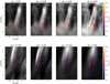 |
Fig. 14. Line-of-sight magnetic field results of the red (top) and blue (bottom) rectangles of the bottom panel of Fig. 7 are overplotted on top of Stokes I at 16:42:44 UT and 17:03:55 UT for the top and bottom panels. The wavelength difference, Δλ, from line centre is shown at the top of each panel. A radial filter (see Skogsrud et al. 2015) has been applied to the images to enhance spicular structures. |
Results of spatially binning and temporally averaging data set 8.
The identification of on-disc BLOS measurements with spicules is more problematic because both the spicules and the underlying chromosphere can contribute to the line formation. Here we compare the spatial distribution of the pixels for which the Bayesian inversion has been performed with photospheric LOS magnetic field data taken with the Helioseismic and Magnetic Imager (HMI; Scherrer et al. 2012; Schou et al. 2012) instrument on board SDO. The hmi.B_45s data products of HMI provide the line-of-sight component of the photospheric magnetic field from observations in the Fe I 6173.3 Å line every 45 s with the HMI Doppler camera. The pixel size of the HMI camera is 0.5″ and for this reason the original image data were interpolated in order to match the pixel scale of CRISP. A comparison between the results of the two instruments is shown in Fig. 15. The values of BLOS are normalised to the maximum value in each data set in order to compare the spatial distribution of the sign of the BLOS values. Only a few on-disc pixels met the asymmetry and correlation criteria described in Sect. 3, rendering the comparison between the results difficult. For this reason, to produce the right panel of Fig. 15 the correlation criterion was lowered, accepting pixels where |R| > 0.6 (while maintaining ε = 0.5 for the asymmetry criterion). As Fig. 15 shows, there is some spatial correlation in the sign distribution of BLOS in the photosphere and in the lower chromosphere. Given that the photospheric magnetic fields in this image delineate the chromospheric network, from which spicules protrude, we have an indication that our on-disc BLOS measurements can be associated with spicules. However, we cannot rule out that a portion of these results come from structures other than spicules.
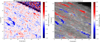 |
Fig. 15. Left: photospheric BLOS obtained with SDO/HMI. Right: BLOS obtained in this work. In each panel the BLOS values have been normalised to their largest respective value in the whole field of view. The observing time is given on top of each image. |
5.3. Height variation of BLOS
The expansion of the magnetic field with increasing height leads to lower magnetic field values in the upper solar atmosphere in comparison with the field present at the photosphere. The LOS magnetic field inferred in the spicules could behave in such a manner, but in this work no clear decrease with height is inferred. The left panel of Fig. 16 shows that if the inferred BLOS from the whole of data set 8 is plotted as a function of the pixel element height, there is no clear correlation between the two values. This was also found in all other off-limb data sets. It is worth noting that Orozco Suárez et al. (2015) detected a decrease of the spicules’ magnetic field strength from 80 G near the limb to 30 G at 3 Mm height (see their Fig. 4). Above this height there is no clear trend in the magnetic field strength, which is in excellent agreement with the behaviour found here. The right panel of Fig. 16 shows the same plot for the chromospheric anemone described in Sect. 4.3. There seems to be a noticeable decrease of BLOS as the distance from the limb increases. This decrease amounts to roughly 100 G in 6 Mm, meaning a BLOS gradient around 16 G Mm−1, which is almost identical to that inferred from the lowest 3 Mm of Fig. 4 of Orozco Suárez et al. (2015).
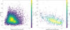 |
Fig. 16. Left: BLOS vs. distance from the limb for all pixels in data set 8. Right: same plot for the chromospheric anemone discussed in Sect. 4.3. The colours in the plot represent the local density of points. |
The difference in the behaviour of BLOS as a function of height for spicules and the anemone could be due to the short length of the former. The signal of spicules comes mostly from heights between 2″ and 5″ above the limb, while the signal from the anemone comes from heights between 4″ and 11″. The anemone is longer, and while at a height of 4″ above the limb both the spicules and the anemone show BLOS values close to 250 G, at 10″ height the values of the latter are close to 150 G. If there were data from spicular material on a wider height range, perhaps the inferred BLOS would behave in a similar manner. Spicules can have longer lengths than those seen at the Ca II 8542 Å line, but they become too faint at upper heights in this line.
5.4. Integration time and pixel scale
As discussed in the Introduction, there are several studies that have tried to infer the magnetic field present in spicular material. However, none of these studies use data with the same exposure time (or integration time in the case of temporal averaging) and pixel scale as the one presented here. Centeno et al. (2010), for example, used data with an effective integration time of 45 minutes and 1″ pixel scale. Orozco Suárez et al. (2015) had a short integration time of 10 s and a spatial resolution of the order of 0.7–1″. Since spicules have a lifetime of a few minutes at most and are thin structures, it is difficult to properly study them with such a cadence and pixel scale.
In order to compare how the results of this study would change if the data used were of lower cadence and larger pixel scale, we performed a spatial binning and temporal integration of two of our data sets (8 and 11). The Bayesian inversion was applied to all pixels of the new data set and then the mode of the BLOS distribution together with the percentage of points that meet the correlation and asymmetry restrictions are presented in Tables 4 and 5 for data sets 8 and 11, respectively. The top left cell in both tables corresponds to the results presented in Sects. 4.1 and 4.2. In the case of off-limb pixels in the vicinity of an active region (Table 4), the value of BLOS for the shortest integration time decreases as the pixel scale is increased. Nevertheless, this behaviour is not found for the other integration times considered and, in general, the BLOS in Table 4 do not depart too much from those computed with the best cadence and pixel scale. It is interesting to note that when the pixel scale is held fixed, then the more exposures that are added, the larger the percentage of pixels that can be used in the Bayesian inversion. This clear trend is not observed when the integration time is fixed and the spatial binning is varied. Regarding on-disc pixels away from an active region (Table 5), we found that both the spatial binning and the temporal integration yield smaller values of BLOS For example, BLOS decreases by a factor of 2.5 if we move along the first row from the best to the worst pixel scale, and by a factor of 4.1 if we move along the first column. Since the percentage of useful pixels increases in both cases, this result looks very solid. A similar behaviour of BLOS with respect to variations of the integration time and pixel scale was found for data set 1 (off-limb and quiet Sun), the change of BLOS along the first row and first column now being 2.30 and 1.54, respectively. It must be mentioned, however, that the statistics of data set 1 is much weaker because the percentages are considerably lower than those in Table 5.
6. Conclusions
In this paper, the Weak Field Approximation (WFA) has been applied for the first time to chromospheric spicules, both on the disc and above the limb. For this purpose we have used spectropolarimetric observations with the SST/CRISP instrument with an exposure time of either 26 s (one data set) or 36 s (five data sets). Given the limitations of the theory and its range of validity, it is clear that a careful treatment of experimental data sets has to be conducted in order to apply the WFA properly. In this study we have translated such limitations into two restrictive criteria, one for the correlation between V(λ) and ∂I(λ)/∂λ and another one for the measured asymmetry of the Stokes V profiles. The imposed criteria result in much less on-disc than off-limb pixels being considered for the calculation of their BLOS, something that was expected given the stronger superposition of spectropolarimetric signals on the disc, where the background chromosphere contributes to the observed Stokes profiles (see Centeno et al. 2010, and Sect. 5.1). This means that the WFA works significantly better for our off-limb observational data sets.
The Bayesian inversion of the Stokes I and V profiles leads to line-of-sight magnetic field components well in excess of 100 G, often reaching as high as 500 G and more. In general, the largest values of BLOS are found in off-limb spicules, probably as a consequence of the much smaller signal superposition, which is stronger on the disc and therefore reduces the BLOS obtained there. Following Centeno et al. (2010), we note that the values presented here are a lower limit of the total magnetic field intensity, for three reasons. The first is quite obvious: having measured just the LOS magnetic field component, the B vector has a larger magnitude than this measurement. Second, we have assumed a filling factor equal to one, but if a pixel has af different from one, then the reported value of BLOS increases by a factor of f−1. Third, the overlapping of emitting off-limb structures or absorbing on-disc structures often reduces the measured BLOS (see Fig. 13).
The BLOS values obtained in this work, most of them at heights between 2″ and 5″ above the limb, are unprecedented and for this reason we have placed them on a firm basis. We have seen that magnetic fields with |BLOS| > 100 G are abundantly present in on-disc and off-limb spicules, both near and away from active regions (see the number of counts in Figs. 8 and 10). We have also provided evidence that the on-disc pixels whose BLOS we have been able to measure are co-spatial with photospheric magnetic field concentrations in the network boundaries and that the magnetic field orientation agrees in the photosphere and in these pixels. This result does not confirm that our on-disc BLOSmeasurements can be unequivocally associated with spicules, but provides a strong basis for this association at least in a considerable number of pixels.
Of the data sets analysed here, five contain off-limb spicules near an active region (data sets 2, 4, 6, 8, and 10); one contains off-limb spicules in the quiet Sun (data set 1); and five more contain on-disc spicules in the quiet Sun (data sets 3, 5, 7, 9, and 11). We establish three statistical comparisons: off-limb active region versus off-limb quiet Sun BLOS values, off-limb quiet Sun versus on-disc quiet Sun BLOS values, and off-limb versus on-disc results. In the first case (off-limb BLOS), Table 2 shows that the BLOS mode of data set 1 (quiet Sun) is of the same order as that of data sets 2, 4, 6, and 8 (active region). Thus, from this small statistical sample we find no evidence of a difference in the average LOS magnetic field strength between quiet Sun spicules and those near an active region, although this conclusion must be confirmed or refuted because we have only studied one data set with off-limb quiet Sun spicules. It is true that the BLOS mode of data set 10 is a factor of 2 larger than that of any other off-limb data set, but we do not know whether this is a statistical anomaly or perhaps the consequence of the spicules in this data set making a small angle with the LOS, which, other things being equal, would lead to larger BLOS values. The large BLOS tails of data set 1 in Fig. 8 compared to those of data sets 2, 4, 6, 8, and 10 could point to larger magnetic field strengths in the quiet Sun, but it could also be a consequence of some spicules in our sample having more inclined magnetic fields with respect to the vertical direction. Regarding the second comparison, namely of quiet Sun BLOS values, Tables 2 and 3 show that off-limb BLOS measurements (data set 1) are of the order of a factor of two larger than on-disc values (data sets 3, 5, 7, 9, and 11). Our simple analysis of the Stokes I and V parameters from two overlapping structures indicates that the WFA can yield a LOS magnetic field strength that is smaller than the largest of the two structures. We suggest (see next paragraph for more details) that on-disc signal superposition has more severe effects than above the limb and that this is the reason for the smaller BLOS measured on the disc. The third comparison is of on-disc and off-limb inversions. The histograms of Fig. 8 have many more points than those of Fig. 10; this fact is also reflected in the top left cells of Tables 4 and 5. This is possibly another side effect of the stronger effect of on-disc signal superposition. Furthermore, the sign of the LOS component of the magnetic field seems to be strongly correlated to the location of the spicules. Those close to a sunspot show a uniform sign equal to that of the sunspot, while spicules located far from a region with a clearly reigning polarity present both BLOS signs (see Orozco Suárez et al. 2015, for a similar conclusion).
Spicules are small scale and very dynamic structures. They appear and fade in a short time and during their existence they can be subject to transverse motions that disturb their position on the plane-of-the-sky and their Doppler velocity. Furthermore, the emission or absorption of several spicules can overlap along a given LOS. Then, during the exposure time, which in our case is the time needed to acquire I, Q, U, and V, the detector records a non-steady signal coming from one or more time-varying structures. This is the reason why long exposure times or the averaging of several exposures, which leads to a long integration time, can corrupt the four Stokes profiles. The same can be said about the spatial binning of data. We have investigated all these effects in Sects. 5.1 and 5.4. In the first one, the two-slab model of Centeno et al. (2010) has been exploited to understand how signal superposition affects the observed Stokes I and V parameters and the determination of BLOS from them. We found that observing two overlapping spicules above the limb leads to either BLOS values that are lower limits to those of the slabs or to Stokes parameters that do not meet the two criteria we impose prior to the application of the Bayesian inversion based on the WFA. In Sect. 5.4 we have proved that the pixel scale and integration time of a data set have a strong influence on the inferred BLOS values and that a coarse spatial and/or temporal resolution lead to smaller BLOS values. This explains why previous works failed to detect such large magnetic fields in spicules in spite of using spectropolarimetric observations, as in this paper. In fact, it is actually surprising that, given the short lifetime of spicules, observations with an integration time of a few minutes (as in Trujillo Bueno et al. 2005) or tens of minutes (Ramelli et al. 2005, 2006; Centeno et al. 2010) enable the calculation of their magnetic field. We put forward the hypothesis that the strong spicular magnetic field, perhaps combined with their possible recurrence in the same position, are responsible for the success of these efforts. We suggest that the spicule magnetic field remains relatively unchanged with time and that spicules are seen as a consequence of density being accumulated by some process (be it a shock, instability, or something else). It is at this moment that the opacity of on-disc spicules or the source function of off-limb spicules is large enough that the spectral line can be detected and the magnetic field can be measured. After some time, the spicular material will disappear, but will reappear in the same flux tube at a later time, allowing one to measure the field again.
The application of the WFA relies on the assumption that, for the spectral line used here, B ≪ 2650 G. This constraint may invalidate the results in the high end of BLOS values, but the bulk of measurements, in the range [50, 300] G, for example, have a high credibility. On the other hand, in the limit of magnetic field strengths below some 50 G, the histograms of Figs. 8 and 10 present a paucity in the number of BLOS inversions. In Sect. 5.1 we have shown that the application of the WFA to Stokes signals from randomly oriented overlapping structures could be the cause of this effect and that the similarity of the distributions of Fig. 10, from observational data on a quiet Sun area, and the middle panel of Fig. 13, from a Monte Carlo experiment, can be a sign of the impact of signal superposition. The results of Sect. 5.1 come from a very idealised model and for this reason one cannot rule out that the combination of noise, spectral resolution, and/or integration time of our data sets may yield poor quality Stokes V signals that prevent the Bayesian inversion from being applied when |BLOS| ≲ 50 G. We thus interpret the distributions of Figs. 8 and 10 as a sign that the WFA applied to our data is biased towards large BLOS and that smaller values do exist but it may not be possible to detect them because of signal superposition, noise in the data, or other factors. Using the WFA to compute the LOS magnetic field component also requires that the magnetic field vector must be uniform along the LOS in each pixel. Superposition along the LOS of several spicules with different B (see e.g. Martínez González et al. 2012) can thus prevent the WFA from being applicable. This is the reason for devising the correlation and asymmetry criteria of Sect. 3.2. The application of these criteria reduces the number of pixels that can be subject to the WFA analysis. Further reduction of this number comes from the fact that some pixels contain material with large Doppler shifts whose Stokes parameters are not well captured by our wavelength grid.
Because of the small range of heights in which the WFA could be applied, we have not been able to assess the possible variation of the BLOS of the spicules with height. Nevertheless, a taller chromospheric anemone present in one of the data sets does show an average gradient of BLOS of the order of 16 G Mm−1. This gradient is very similar to that obtained by Orozco Suárez et al. (2015) in the lowest 3 Mm of spicules.
The results presented here should be tested by observing spicules in other locations and with other instruments. We anticipate that their confirmation will arrive with the Daniel K. Inouye Telescope in the near future.
This is the most restrictive microturbulent velocity value we have found in the literature for the Ca II 8542 Å line. Figure 11 of Vernazza et al. (1981) gives ξ = 5 km s−1 at 1500 km height. Both de la Cruz Rodríguez et al. (2013) and Quintero Noda et al. (2016) use ξ = 3 km s−1. Finally, Jurčák et al. (2018) quote values in the range 4–5 km s−1 and 3.5–13 km s−1 for VAL (Vernazza et al. 1981) and FAL (Fontenla et al. 1993) models, respectively.
To see how much asymmetry is allowed by this value, see Fig. 5.
The BIC is best suited for situations in which the number of sampled points, i.e. the number of wavelengths, is much larger than the number of free parameters in the models. In our case, we have either 15 or 21 sampled points and four or six free parameters depending on the model. Hence, the ratio between the number of free parameters and the number of sampled points is in the range [0.2, 0.4]. Such ratios may appear to be large but in all cases the BIC difference between the two models is larger than six, which means that the evidence against the model with the highest BIC value is at least strong.
Acknowledgments
MK and RO acknowledge support from the Spanish Ministry of Economy and Competitiveness (MINECO) and FEDER funds through project AYA2017-85465-P. They are also grateful for the travel support received from the International Space Science Institute (Bern, Switzerland) as well as for discussions with members of the ISSI team on “Observed multi-scale variability of coronal loops as a probe of coronal heating”, led by C. Froment and P. Antolin. PA acknowledges funding from his STFC Ernest Rutherford Fellowship (No. ST/R004285/2). This research has made use of SunPy v1.1, an open-source and free community-developed solar data analysis Python package (The SunPy Community 2020). The Swedish 1-m Solar Telescope is operated on the island of La Palma by the Institute for Solar Physics of Stockholm University in the Spanish Observatorio del Roque de los Muchachos of the Instituto de Astrofísica de Canarias. The Institute for Solar Physics is supported by a grant for research infrastructures of national importance from the Swedish Research Council (registration number 2017-00625). D.K. has received funding from the Sêr Cymru II scheme, part-funded by the European Regional Development Fund through the Welsh Government and from the Georgian Shota Rustaveli National Science Foundation project FR17 323. AAR acknowledges support from the Spanish Ministry of Economy and Competitiveness (MINECO) and FEDER funds through project PGC2018-102108-B-I00. And last but not least, we thank the anonymous referee for very useful comments.
References
- Asensio Ramos, A. 2011, ApJ, 731, 27 [NASA ADS] [CrossRef] [Google Scholar]
- Asensio Ramos, A., Trujillo Bueno, J., & Landi Degl’Innocenti, E. 2008, ApJ, 683, 542 [NASA ADS] [CrossRef] [Google Scholar]
- Auer, L. H., & Heasley, J. N. 1978, A&A, 64, 67 [NASA ADS] [Google Scholar]
- Beckers, J. M. 1968, Sol. Phys., 3, 367 [NASA ADS] [Google Scholar]
- Bose, S., Henriques, V. M. J., Rouppe van der Voort, L., & Joshi, J. 2019, A&A, 631, L5 [CrossRef] [EDP Sciences] [Google Scholar]
- Centeno, R. 2018, ApJ, 866, 89 [NASA ADS] [CrossRef] [Google Scholar]
- Centeno, R., Trujillo Bueno, J., & Asensio Ramos, A. 2010, ApJ, 708, 1579 [NASA ADS] [CrossRef] [Google Scholar]
- Collados, M., Lagg, A., Díaz García, J. J., et al. 2007, in Tenerife Infrared Polarimeter II, eds. P. Heinzel, I. Dorotovič, R. J. Rutten, et al., ASP Conf. Ser., 368, 611 [Google Scholar]
- de la Cruz Rodríguez, J., & van Noort, M. 2017, Space Sci. Rev., 210, 109 [NASA ADS] [CrossRef] [Google Scholar]
- de la Cruz Rodríguez, J., Rouppe van der Voort, L., Socas-Navarro, H., & van Noort, M. 2013, A&A, 556, A115 [NASA ADS] [CrossRef] [EDP Sciences] [Google Scholar]
- de la Cruz Rodríguez, J., Löfdahl, M. G., Sütterlin, P., Hillberg, T., & Rouppe van der Voort, L. 2015, A&A, 573, A40 [NASA ADS] [CrossRef] [EDP Sciences] [Google Scholar]
- De Pontieu, B., McIntosh, S. W., Carlsson, M., et al. 2007, Science, 318, 1574 [NASA ADS] [CrossRef] [PubMed] [Google Scholar]
- De Pontieu, B., McIntosh, S. W., Carlsson, M., et al. 2011, Science, 331, 55 [NASA ADS] [CrossRef] [Google Scholar]
- De Pontieu, B., Martinez-Sykora, J., De Moortel, I., Chintzoglou, G., & McIntosh, S. W. 2017, AGU Fall Meeting Abstracts, 2017 SH43A-2793 [Google Scholar]
- Elmore, D. F., Lites, B. W., Tomczyk, S., et al. 1992, in The Advanced Stokes Polarimeter – A New Instrument for Solar Magnetic Field Research, eds. D. H. Goldstein, R. A. Chipman, et al., SPIE Conf. Ser., 1746, 22 [Google Scholar]
- Fontenla, J. M., Avrett, E. H., & Loeser, R. 1993, ApJ, 406, 319 [Google Scholar]
- Gandorfer, A. M., Steiner, H. P. P. P., Aebersold, F., et al. 2004, A&A, 422, 703 [NASA ADS] [CrossRef] [EDP Sciences] [Google Scholar]
- Harvey, J. W. 2012, Sol. Phys., 280, 69 [CrossRef] [Google Scholar]
- Henriques, V. M. J. 2012, A&A, 548, A114 [NASA ADS] [CrossRef] [EDP Sciences] [Google Scholar]
- Henriques, V. M. J., Kuridze, D., Mathioudakis, M., & Keenan, F. P. 2016, ApJ, 820, 124 [NASA ADS] [CrossRef] [Google Scholar]
- Hinode Review Team (Al-Janabi, K., et al.) 2019, PASJ, 71, R1 [CrossRef] [Google Scholar]
- Jennerholm Hammar, F. 2014, Master’s thesis, Uppsala Universitet, Sweden [Google Scholar]
- Jurčák, J., Štěpán, J., Trujillo Bueno, J., & Bianda, M. 2018, A&A, 619, A60 [CrossRef] [EDP Sciences] [Google Scholar]
- Kosugi, T., Matsuzaki, K., Sakao, T., et al. 2007, Sol. Phys., 243, 3 [Google Scholar]
- Kuridze, D., Mathioudakis, M., Simões, P. J. A., et al. 2015, ApJ, 813, 125 [NASA ADS] [CrossRef] [Google Scholar]
- Kuridze, D., Henriques, V. M. J., Mathioudakis, M., et al. 2018, ApJ, 860, 10 [NASA ADS] [CrossRef] [Google Scholar]
- Kuridze, D., Mathioudakis, M., Morgan, H., et al. 2019, ApJ, 874, 126 [NASA ADS] [CrossRef] [Google Scholar]
- Landi Degl’Innocenti, E. 1982, Sol. Phys., 77, 285 [NASA ADS] [CrossRef] [Google Scholar]
- Landi Degl’Innocenti, A., & Landolfi, M. 2004, Polarization in Spectral Lines (Kluwer Academic Publishers) [Google Scholar]
- Lemen, J. R., Title, A. M., Akin, D. J., et al. 2012, Sol. Phys., 275, 17 [Google Scholar]
- López Ariste, A., & Casini, R. 2005, A&A, 436, 325 [NASA ADS] [CrossRef] [EDP Sciences] [Google Scholar]
- Martínez González, M. J., Asensio Ramos, A., Manso Sainz, R., Beck, C., & Belluzzi, L. 2012, ApJ, 759, 16 [NASA ADS] [CrossRef] [Google Scholar]
- Martínez Pillet, V., & Collados, M. 1999, in LPSP & TIP: Full Stokes Polarimeters for the Canary Islands Observatories, eds. T. R. Rimmele, K. S. Balasubramaniam, & R. R. Radick, ASP Conf. Ser., 183, 264 [Google Scholar]
- Orozco Suárez, D., Asensio Ramos, A., & Trujillo Bueno, J. 2015, ApJ, 803, L18 [NASA ADS] [CrossRef] [Google Scholar]
- Pearson, K., & Galton, F. 1895, Proc. R. Soc. London, 58, 240 [Google Scholar]
- Pereira, T. M. D., De Pontieu, B., & Carlsson, M. 2012, ApJ, 759, 18 [NASA ADS] [CrossRef] [Google Scholar]
- Pereira, T. M. D., De Pontieu, B., Carlsson, M., et al. 2014, ApJ, 792, L15 [NASA ADS] [CrossRef] [Google Scholar]
- Pietarila, A., Socas-Navarro, H., & Bogdan, T. 2007, ApJ, 663, 1386 [Google Scholar]
- Quintero Noda, C., Shimizu, T., de la Cruz Rodríguez, J., et al. 2016, MNRAS, 459, 3363 [NASA ADS] [CrossRef] [Google Scholar]
- Ramelli, R., Bianda, M., Trujillo Bueno, J., et al. 2005, in Chromospheric and Coronal Magnetic Fields, eds. D. E. Innes, A. Lagg, S. A. Solanki, et al., ESA Spec. Publ., 596, 82.1 [Google Scholar]
- Ramelli, R., Bianda, M., Merenda, L., & Trujillo Bueno, T. 2006, in The Hanle and Zeeman Effects in Solar Spicules, eds. R. Casini, & B. W. Lites, ASP Conf. Ser., 358, 448 [Google Scholar]
- Rouppe van der Voort, L. H. M., De Pontieu, B., Hansteen, V. H., Carlsson, M., & van Noort, M. 2007, ApJ, 660, L169 [NASA ADS] [CrossRef] [Google Scholar]
- Rouppe van der Voort, L., Leenaarts, J., de Pontieu, B., Carlsson, M., & Vissers, G. 2009, ApJ, 705, 272 [NASA ADS] [CrossRef] [Google Scholar]
- Rutten, R. J. 2012, Philos. Trans. R. Soc. London Ser. A, 370, 3129 [Google Scholar]
- Sainz Dalda, A., & López Ariste, A. 2007, A&A, 469, 721 [NASA ADS] [CrossRef] [EDP Sciences] [Google Scholar]
- Salvatier, J., Wiecki, T. V., & Fonnesbeck, C. 2016, PyMC3: Python probabilistic programming framework [Google Scholar]
- Scharmer, G. B., Bjelksjo, K., Korhonen, T. K., Lindberg, B., & Petterson, B. 2003, The 1-m Swedish Solar Telescope [Google Scholar]
- Scharmer, G. B., Narayan, G., Hillberg, T., et al. 2008, ApJ, 689, L69 [Google Scholar]
- Scherrer, P. H., Schou, J., Bush, R. I., et al. 2012, Sol. Phys., 275, 207 [Google Scholar]
- Schou, J., Scherrer, P. H., Bush, R. I., et al. 2012, Sol. Phys., 275, 229 [Google Scholar]
- Schwarz, G. 1978, Ann. Stat., 6, 461 [Google Scholar]
- Secchi, A. 1877, Le Soleil, 2 (Paris: Gauthier-villars) [Google Scholar]
- Sheminova, V. A. 2005, Kinematika i Fizika Nebesnykh Tel, 21, 172 [Google Scholar]
- Shibata, K., Nakamura, T., Matsumoto, T., et al. 2007, Science, 318, 1591 [NASA ADS] [CrossRef] [Google Scholar]
- Sigwarth, M. 2001, ApJ, 563, 1031 [NASA ADS] [CrossRef] [Google Scholar]
- Skogsrud, H., Rouppe van der Voort, L., De Pontieu, B., & Pereira, T. M. D. 2015, ApJ, 806, 170 [NASA ADS] [CrossRef] [Google Scholar]
- Socas-Navarro, H., & Elmore, D. 2005, ApJ, 619, L195 [NASA ADS] [CrossRef] [Google Scholar]
- Solanki, S. K. 1993, Space Sci. Rev., 63, 1 [NASA ADS] [CrossRef] [Google Scholar]
- Sterling, A. C. 2000, Sol. Phys., 196, 79 [NASA ADS] [CrossRef] [Google Scholar]
- Suematsu, Y., Tsuneta, S., Ichimoto, K., et al. 2008, Sol. Phys., 249, 197 [NASA ADS] [CrossRef] [Google Scholar]
- The SunPy Community (Barnes, W. T., et al.) 2020, ApJ, 890, 68 [CrossRef] [Google Scholar]
- Trujillo Bueno, J., Merenda, L., Centeno, R., Collados, M., & Landi Degl’Innocenti, E. 2005, ApJ, 619, L191 [NASA ADS] [CrossRef] [Google Scholar]
- Tsiropoula, G., Tziotziou, K., Kontogiannis, I., et al. 2012, Space Sci. Rev., 169, 181 [NASA ADS] [CrossRef] [Google Scholar]
- Van Noort, M., Der Voort, L. R. V., & Löfdahl, M. G. 2005, Sol. Phys., 228, 191 [NASA ADS] [CrossRef] [Google Scholar]
- Vernazza, J. E., Avrett, E. H., & Loeser, R. 1981, ApJS, 45, 635 [Google Scholar]
- Yurchyshyn, V., Cao, W., Abramenko, V., Yang, X., & Cho, K.-S. 2020, ApJ, 891, L21 [CrossRef] [Google Scholar]
All Tables
All Figures
|
Fig. 1. Context of the observations of 03 June 2016 at 16:27 UT. The top panel shows the CRISP field of view (blue square) on an SDO/AIA image in the 171 Å filter. The middle panel shows a zoomed view of the top panel. The bottom panel shows a nearly co-temporal SST/CRISP image in the line centre of the Ca II 8542 Å line. Time is shown at the top of each frame and solar north is to the top. |
| In the text | |
|
Fig. 2. Stokes parameters at line centre on 03 June 2016 at 16:27:42 UT. The parameters are normalised to the continuum intensity, Ic, measured as the average of I on the disc at the line wings (|Δλ| > 1.25 Å). Solar north is to the left. |
| In the text | |
|
Fig. 3. Typical asymmetric Stokes V profile (from Sheminova 2005). The meaning of the various quantities is given in the text. |
| In the text | |
|
Fig. 4. Stokes V against ∂I/∂λ for a pixel in which |R| < 0.9 (left) and a pixel in which |R| > 0.9. The corresponding values of R are shown on top of each panel. |
| In the text | |
|
Fig. 5. Examples of Stokes V profiles in which the correlation criterion |R| > 0.9 is met. Left: the asymmetry criterion is not satisfied. Right: the asymmetry criterion is satisfied. The insets show the plots of Stokes V vs. ∂I/∂λ, both of which have passed the filter |R| > 0.9. |
| In the text | |
|
Fig. 6. Results of the Bayesian inference for one pixel. The mode of the posterior distribution and the 95% HPD interval of BLOS (left; in Gauss) and σ (right; in normalised count units) are shown. |
| In the text | |
|
Fig. 7. Results from the Bayesian inference for the off-limb data of 02 June 2016 at 07:46:06 UT, belonging to data set 1 (top frame), and 03 June 2016 at 16:43:20 UT, belonging to data set 8 (bottom frame). The points are coloured based on the mode from the posterior distribution of the LOS magnetic field intensity (see colour bar at the right) and are plotted on top of the Ca II 8542 Å line centre intensity image. The blue line represents the position of the solar limb, while the black and yellow curves represent the heights 2″ and 5″ above the limb, respectively. The red and blue rectangles in the bottom panel are used in Fig. 14. |
| In the text | |
|
Fig. 8. Histogram of BLOS values for the off-limb pixels. The data set labels are those given in Table 1. |
| In the text | |
|
Fig. 9. Schematic representation of the magnetic polarity of AR 12551 and the spicule fields (short blue and red arrows) around the dominant magnetic polarities (long blue and red arrows). The green and black straight lines respectively represent the line-of-sight tangent to the solar limb of data sets 2, 4, and 6 (morning of 03 June 2016), and of data set 8 (afternoon of 03 June 2016). |
| In the text | |
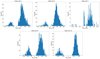 |
Fig. 10. Same as Fig. 8 for on-disc pixels. The data set labels are those given in Table 1. |
| In the text | |
|
Fig. 11. Chromospheric anemone observed on 03 June 2016 at 16:31:50 UT, viewed in the Ca II 8542 Å line centre (left) and −0.75 Å from line centre (right). |
| In the text | |
|
Fig. 12. Temporal evolution of the chromospheric anemone seen in Fig. 11 and the inferred BLOS values. The leftmost picture was taken on 03 June 2016 at 16:31:50 UT and the subsequent figures show the evolution of the region and the inferred BLOS at time intervals of 36.33 s. |
| In the text | |
|
Fig. 13. Results of the WFA BLOS inversion when the Stokes I and V parameters in a pixel come from two overlapping structures (cf. Eqs. (10) and (11)). Top: BLOS normalised by dividing it by the maximum LOS magnetic field of the two structures, in absolute value. It is plotted vs. the difference between the two slabs’ Doppler velocity, ΔvD, for several intensity amplitude ratios, I02/I01. The dashed black lines give the results for which |R| > 0.9. In this plot BLOS1 = 200 G and BLOS2 = −40 G. Middle: BLOS distribution from the Monte Carlo experiment. Bottom: BLOS distribution divided by the maximum of |BLOS1|,|BLOS2|. In the middle and bottom panels, the blue and beige colours respectively correspond to all the samples in the Monte Carlo experiment and only those that pass the filter |R| > 0.9. |
| In the text | |
|
Fig. 14. Line-of-sight magnetic field results of the red (top) and blue (bottom) rectangles of the bottom panel of Fig. 7 are overplotted on top of Stokes I at 16:42:44 UT and 17:03:55 UT for the top and bottom panels. The wavelength difference, Δλ, from line centre is shown at the top of each panel. A radial filter (see Skogsrud et al. 2015) has been applied to the images to enhance spicular structures. |
| In the text | |
|
Fig. 15. Left: photospheric BLOS obtained with SDO/HMI. Right: BLOS obtained in this work. In each panel the BLOS values have been normalised to their largest respective value in the whole field of view. The observing time is given on top of each image. |
| In the text | |
|
Fig. 16. Left: BLOS vs. distance from the limb for all pixels in data set 8. Right: same plot for the chromospheric anemone discussed in Sect. 4.3. The colours in the plot represent the local density of points. |
| In the text | |
Current usage metrics show cumulative count of Article Views (full-text article views including HTML views, PDF and ePub downloads, according to the available data) and Abstracts Views on Vision4Press platform.
Data correspond to usage on the plateform after 2015. The current usage metrics is available 48-96 hours after online publication and is updated daily on week days.
Initial download of the metrics may take a while.