| Issue |
A&A
Volume 642, October 2020
|
|
|---|---|---|
| Article Number | A23 | |
| Number of page(s) | 10 | |
| Section | Planets and planetary systems | |
| DOI | https://doi.org/10.1051/0004-6361/202038332 | |
| Published online | 30 September 2020 | |
Ejection of close-in super-Earths around low-mass stars in the giant impact stage
1
Institute of Astronomy and Astrophysics,
Academia Sinica,
Taipei
10617, Taiwan
e-mail: This email address is being protected from spambots. You need JavaScript enabled to view it.
2
National Astronomical Observatory of Japan,
2-21-1, Osawa, Mitaka,
181-8588
Tokyo, Japan
3
Institute for Cosmic Ray Research, University of Tokyo,
Hida,
Gifu
506-1205, Japan
4
Astrobiology Center, NINS,
2-21-1, Osawa, Mitaka,
181-8588
Tokyo, Japan
Received:
4
May
2020
Accepted:
23
July
2020
Abstract
Context. Earth-sized planets were observed in close-in orbits around M dwarfs. While more and more planets are expected to be uncovered around M dwarfs, theories of their formation and dynamical evolution are still in their infancy.
Aims. We investigate the giant impact stage for the growth of protoplanets, which includes strong scattering around low-mass stars. The aim is to clarify whether strong scattering around low-mass stars affects the orbital and mass distributions of the planets.
Methods. We performed an N-body simulation of protoplanets by systematically surveying the parameter space of the stellar mass and surface density of protoplanets.
Results. We find that protoplanets are often ejected after twice or three times the close-scattering around late M dwarfs. The ejection sets the upper limit of the largest planet mass. By adopting the surface density that linearly scales with the stellar mass, we find that as the stellar mass decreases, less massive planets are formed in orbits with higher eccentricities and inclinations. Under this scaling, we also find that a few close-in protoplanets are generally ejected.
Conclusions. The ejection of protoplanets plays an important role in the mass distribution of super-Earths around late M dwarfs. The mass relation of observed close-in super-Earths and their central star mass is reproduced well by ejection.
Key words: planets and satellites: dynamical evolution and stability / planets and satellites: formation
© ESO 2020
1 Introduction
Recent observations have reported the presence of planets around M dwarfs with a mass of ~0.1 M⊙, where M⊙ is the Solar mass (Anglada-Escudé et al. 2016; Gillon et al. 2017; Zechmeister et al. 2019). These planets are located within 0.1 au, and their masses are around the mass of the Earth. In addition to these planets, almost dozens of planets are found around stars with ≲0.3 M⊙ (e.g., Hirano et al. 2016; Angelo et al. 2017; Bonfils et al. 2018). Since planet occurrence rates tend to be high around low-mass stars (Dressing & Charbonneau 2013, 2015; Hardegree-Ullman et al. 2019), ongoing and upcoming observational missions are expected to find more and more planets around M dwarfs. Figure 1 shows the mass relation of observed planets and their central stars. This figure clearly shows that low-mass stars have small mass planets and there are not any ~10 Earth-mass planets around ~0.1 M⊙ stars, while these types of mass planets are abundant around 1 M⊙ stars. In this paper, we focus on the mass relation between the stars and these planets, which have ≲10 M⊕ and are located at ≲1 au, where M⊕ is the Earth mass. We refer to these planets as close-in super-Earths. It is worth noting that this mass gap of close-in super-Earths exists around ≲0.5 M⊙ stars and no planets have been reported by the Kepler mission around these types of stars since these planets are orbiting around >0.5 M⊙ stars (Johnson et al. 2017; Weiss et al. 2018a,b).
The formation of close-in super-Earths is composed of various processes (e.g., Raymond et al. 2014; Raymond & Morbidelli 2020). Their formation can be divided into the following two stages: the formation of protoplanets and their giant impact growth. Protoplanets grow by the accretion of planetesimals (e.g., Wetherill & Stewart 1989; Kokubo & Ida 1996, 1998, 2000) and/or pebbles (e.g., Ormel & Klahr 2010; Lambrechts & Johansen 2012; Johansen & Lambrechts 2017). These protoplanets originally grow either in the close-in orbit (e.g., Ogihara et al. 2015; Ogihara & Hori 2020) or in the outer region (e.g., Kley & Nelson 2012; Rein 2012). Due to the planet-disk tidal interaction (e.g., Ward 1986; Tanaka et al. 2002; Ida et al. 2020), they are trapped in resonant chains around the inner edge of the disk. When there are few protoplanets in the resonant chain, they do not cause giant impacts, and planets are formed in resonant chain orbits. When there are several protoplanets, they cause orbital instabilities and giant impacts occur (e.g., Ogihara & Ida 2009; Matsumoto et al. 2012; Matsumoto & Ogihara 2020). We note that most planets are considered to have evolved according to the later scenario since they are not in resonant chains (Fabrycky et al. 2014; Winn & Fabrycky 2015). The distribution of protoplanets affects the distribution of planets since it determines whether giant impacts occur. Recent studies have shown that the distributions of protoplanets and subsequently formed planets are affected by the main accretion source (planetesimals or pebbles) and gas removal processes (e.g., Ogihara et al. 2018; Izidoro et al. 2017, 2019; Ogihara & Hori 2020).
Most of these theoretical studies considered the formation of close-in super-Earths around 1 M⊙ stars, and the distribution of protoplanets around M dwarfs is not well known. Recently, Liu et al. (2019, 2020) have shown that small planets form around low-mass stars when they grow via pebble-driven core accretion. These studies focus on the formation stage of protoplanets. They consider the growth of a single protoplanet, and the distribution of protoplanets in a system is not clear.
The growth of protoplanets through giant impacts has also mainly been studied around 1 M⊙ stars (e.g., Kokubo et al. 2006; Hansen & Murray 2012, 2013; Matsumoto & Kokubo 2017). The dynamical process in the giant impact stage around M dwarfs is not well known since no studies to date have considered the systematical survey on the parameter space composed of the stellar mass and protoplanet mass, whereas some studies have considered the dependence of the stellar mass on the giant impact growth as follows. Lissauer (2007) performed N-body simulations of planetesimals and protoplanets around the habitable zone of (1∕3) M⊙. The planetary accretion around the habitable zone of M dwarfs was also investigated by Raymond et al. (2007). They considered the stellar mass to be a parameter ranging from 0.2 M⊙ to 1 M⊙. Ciesla et al. (2015) also performed simulations in the same stellar mass range. Montgomery & Laughlin (2009) considered the growth of planetary embryos around 0.12 M⊙ stars. Ogihara & Ida (2009) performed N-body simulations of planetesimals, considering orbital migration around 0.2 M⊙. Moriarty & Ballard (2016) examined the planetary accretion around 1 M⊙ and 0.5 M⊙ to reproduce the distribution of planets that exhibits the so-called Kepler dichotomy found by the Kepler mission (Johansen et al. 2012).
In this paper, we focus on the in-situ formation of close-in super-Earths via giant impacts around low-mass stars to consider the planet mass distribution around low-mass stars (Fig. 1). We systematically changed the stellar mass between 1 M⊙ and 10−5∕4 M⊙≃ 0.056 M⊙. The lowest stellar mass in our parameter range is in the mass range of brown dwarfs (Reid & Hawley 2005). We initially put isolation mass protoplanets in a gas-free disk (Kokubo & Ida 2000, 2002). The corresponding disk surface densities are 10–100 g cm−2 at 1 au. While these densities are more massive than the surface densities suggested by observations (e.g., Williams & Cieza 2011; Andrews et al. 2013), we used these surface densities to reproduce ~ 1 M⊕ to ~ 10 M⊕ planets (see Manara et al. 2018, for more detailed comparisons of the observed dust mass and observed planet mass). As the stellar mass decreases, scattering between protoplanets becomes relatively strong for a given mass of protoplanets. Our results show that this type of strong scattering causes protoplanet ejections from M dwarfs. These ejection events provide a possible explanation for the planet-stellar mass relation around low-mass stars as to why there are not any ~ 10 Earth-mass planets around ~0.1 M⊙ stars.
This paper is organized as follows. Our numerical model is described in Sect. 2. We show how the stellar mass and surface density affect the final orbital and mass distributions of planets in Sect. 3. Section 4 presents our conclusions.
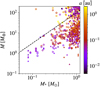 |
Fig. 1 Distribution of observed planets on the stellar mass in the solar mass unit (M* [M⊙]) and planetary mass in the Earth mass unit (M [M⊕]) plane. The data were extracted from the NASA exoplanet archive (https://exoplanetarchive.ipac.caltech.edu/) as of April 2020. Point colors represent the semimajor axis of each planet. Planets shown in circles were detected by the radial velocity (RV) method and those in triangles were detected using the transit or transit timing methods. The dashed line is the ejection mass at 0.1 au, given by Eq. (4). |
2 Numerical model
2.1 Initial conditions
We consider the giant impact growth of protoplanets around a star whose mass is M* without disk gas. The stellar mass (M*) ranges from 1 M⊙ to 10−5∕4 M⊙. This parameter range of the stellar mass includes the mass range of M dwarfs (Reid & Hawley 2005; Kaltenegger & Traub 2009) and the ultra-cool stars where planets have been observed (Gillon et al. 2017; Zechmeister et al. 2019).
The mass distribution of protoplanets that are precursors to close-in super-Earths is still under debate. In this study, we assume that protoplanets initially have isolation masses (Kokubo & Ida 2000, 2002). It is important to note that we are not implying that protoplanets in close-in orbits form according to the oligarchic model. We adopt the isolation mass model since this model gives us a relation between protoplanet masses and surface density. The surface density of protoplanets is given by the power-law disk model, 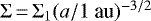 , for which the power index was taken from the minimum-mass solar nebular model (Hayashi 1981). This power-law index is slightly larger than those derived from observed close-in super-Earths by Chiang & Laughlin (2013) (− 1.6) and Dai et al. (2020) (− 1.75). The protoplanets are initially located at a = (0.05 au, 1 au), where a is the semimajor axis of a protoplanet. We placed the innermost protoplanet at 0.05 au + 0.5binit. The semimajor axes of the other planets are given by ai+1 = ai + binit within 1 au. The initial orbital separation is a parameter and its fiducial value is binit = 10rH, where rH is the Hill radius of a protoplanet (
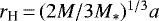 ). The initial masses of protoplanets are given by (Kokubo & Ida 2000, 2002)
 (1)
(1)
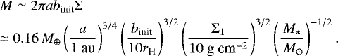
The total mass of the initial protoplanets (Mtot,init) is almost equal to
 (2)
(2)
which was obtained by the integration of the surface density between 0.05 and 1 au. The surface density at 1 au (Σ1) is a parameter in our simulations. In this study, we focus on the planet mass range of ~ 1 M⊕–10 M⊕. As Matsumoto & Kokubo (2017) demonstrate, it is expected that several similar mass planets form in close-in orbits. Accordingly, we used Σ1 = 10, 30, and 100 g cm−2.
Each model in our simulations is named after M*, Σ1, and b. For instance, Ms0Σ100b10 is the model for M* = 100 M⊙, Σ1 = 100 g cm−2, and binit = 10rH. All of the models in our simulations are summarized in Table 1. We calculated 20 runs in each model by randomly changing the initial angles of protoplanets.
As the stellar mass decreases, the mass of the initial protoplanet increases (see Eq. (1)), while the number of initial protoplanets (ninit) decreases since the Hill radius increases ( ) and ninit is roughly proportional to
  . The number of initial protoplanets is the smallest, that is ninit = 6, in the Ms5Σ100b10 model. Whereas, it is the largest, that is ninit = 67, in the Ms0Σ10b10 model. To evaluate the effects of ninit and the initial value of M on the results, we also performed simulations with binit = 8rH and 6rH for M* = 10−5∕4 M⊙ and Σ1 = 100 g cm−2, respectively (models Ms5Σ100b8 and Ms5Σ100b6 in Table 1). The initial eccentricities (e) and inclinations (i [rad]) are given by the Rayleigh distribution with the dispersions
  , which are proportional to
  . It is worth noting that Matsumoto & Kokubo (2017) show that the initial eccentricities of protoplanets do not affect the results and the initial inclinations only affect the results when they change in orders of magnitudes.
Summary of models.
2.2 Orbital integration
The orbital motions of protoplanets are calculated by the direct integration of their equations of motion. We used the fourth-order Hermite scheme (Makino & Aarseth 1992; Kokubo & Makino 2004) with the hierarchical timestep (Makino 1991). The maximum timesteps are almost equal to 0.01TK of the innermost planet, where TK is the Keplerian time. This is about 1 h for a planet at 0.05 au around a 1 M⊙ star and 0.2 h for one at 0.05 au around a 10−5∕4 M⊙ star. These types of short timesteps enable us to precisely resolve collisions of protoplanets, which are important for the collisional damping of eccentricities and inclinations (Matsumoto et al. 2015; Matsumoto & Kokubo 2017). By adopting this timescale, the error in the total energy in TK of the innermost planet was  when we simulated one protoplanet.
We followed the evolution for at least 107 yr. After 107 yr, we estimated the orbital crossing time of the system using the minimum orbital crossing time derived by Ida & Lin (2010) (see also Appendix A). We continued the integration until the crossing time was longer than 107 yr or the orbital elements were almost constant in the last 107 yr. In some calculations, we continued the simulations over 108 yr and can confirm that they do not lead to orbital instabilities. This is because the accretion timescale in the giant impact stage is ~ 108TK – 109 TK (Agnor et al. 1999; Kokubo et al. 2006; Hansen & Murray 2012; Moriarty & Ballard 2016). We assume perfect accretion; namely, when protoplanets collide, they always merge. Protoplanets have the same bulk density, ρ = 3 g cm−3.
3 Results
3.1 Typical evolution
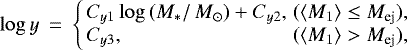
Although the disk properties are the same, the orbital evolution of protoplanets significantly differed when we changed the stellar mass. Figure 2 shows the time evolution of the semimajor axes as well as pericenter and apocenter distances in models Ms0Σ100b10 (left panel, M* = 1 M⊙) and Ms5Σ100b10 (right one, M* = 10−5∕4 M⊙), respectively.In these models, the total masses of the initial protoplanets are about 37 M⊕. In the Ms0Σ100b10 model, orbital crossing occurs from smaller orbital radii due to the shorter orbital periods. Most of the collisions occur soon after orbital crossing, which results in the tournament-like structure of the time evolution of the semimajor axes (Matsumoto & Kokubo 2017). In this case, four planets finally form. The mass of the innermost planet is 5.1 M⊕ and those of the other three planets are between 10 M⊕ and 12 M⊕. The eccentricities (e) and inclinations (i) of the planets are 0.15, 0.097, 0.076, and 0.10 and 0.091, 0.0514, 0.12, and 0.088 rad starting from the innermost planets, respectively. The estimated crossing timescale of the final planets is longer than 1010 yr. Except for the innermost scattered planet, planets have a similar mass and small eccentricities (≤ 0.1). The final eccentricities of planets are given by the close-scattering and collisional damping when inclinations of initial protoplanets are small (Matsumoto et al. 2015; Matsumoto & Kokubo 2017). The eccentricity raised in a close-scattering event is given by the fraction of the escape velocity to the Kepler velocity,
 (3)
(3)
which is often referred to as the escape eccentricity (Safronov 1972; Kokubo & Ida 2002; Leinhardt & Richardson 2005; Pfyffer et al. 2015; Matsumoto et al. 2015; Matsumoto & Kokubo 2017). The eccentricity of the scattered innermost planet is ~ eesc, and those of the other planets are ~0.5eesc due to the collisional e-damping.
This type of tournament-like structure is not seen in the Ms5Σ100b10 model. Scattering between protoplanets becomes more prominent as the stellar mass decreases since their Hill radii become larger. Protoplanets tend to scatter away from each other rather than collide. Strong scattering leads to protoplanet ejections. In the right panel of Fig. 2, two ejection events occur. The first ejection occurs at 4.2 × 10⁴ yr. While the semimajor axis of the first ejected body (the solid red curve) exceeds 10 au at 1.3 × 10⁴ yr; its pericenter (the red-dashed curve) stays at ≲1 au since its eccentricity is e > 0.9. Its eccentricity exceeds unity due to scattering with other protoplanets at 4.2 × 10⁴ yr. The second ejection happens at 1.8 × 10⁵ yr. The semimajor axis of the second ejected body (the solid blue curve) drastically changes several times due to scattering. This body is ejected by multiple scattering with the outermost planet (the brown curve). Finally, two planets form. The inner one has M = 19 M⊕, e = 0.18, and i = 0.41 rad. The outer one has M = 15 M⊕, e = 0.26, and i = 0.22 rad. These final eccentricities of planets are less than 0.3eesc.
The dynamical evolution of close-in super-Earths around ~ 0.1 M⊙ stars is similar to that of giant planets around 1 M⊙ stars (e.g., Rasio & Ford 1996; Marzari & Weidenschilling 2002; Nagasawa et al. 2008). Strong scattering between protoplanets leads to ejection. Around low-mass stars, gravitational scattering between protoplanets is strong due to their large initial mass (Eq. (1)) and the weak stellar gravity. Protoplanets around low-mass stars easily gain high eccentricities ( ), and some are subsequently ejected. Although the two ejected bodies (the red and blue ones) acquire high eccentricities e ~ eesc > 0.9, they are not immediately ejected after their orbits are crossed. Their pericenters stay around the semimajor axis of the outermost body (the brown one). These are scattered again, and their eccentricities exceed unity. Therefore, protoplanets are ejected by multiple close-scattering events even when eesc is smaller than unity. The giant impact growth of protoplanets is regulated by ejection due to multiple scattering events as the stellar mass becomes low.
 |
Fig. 2 Typical time evolution is shown for models Ms0Σ100b10 (left, M* = 1 M⊙) and Ms5Σ100b10 (right, M* = 10−5∕4 M⊙). The solid and dashed curves in the same color show the semimajor axis as well as pericenter and apocenter distances of each body. When two protoplanets collide, the merged body has the same color as that of the massive protoplanet. |
3.2 The collision-dominated regime and ejection-dominated regime
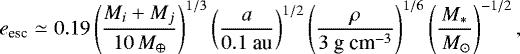
As the stellar mass decreases, eesc increases and planetary scattering becomes more effective. This promotes planetary growth via giant impacts. However, when eesc exceeds a certain value, the ejection becomes effective and planets do not grow via giant impacts. These features can be seen in Fig. 3. The left and right panels of Fig. 3 show the mass of the most massive planets (⟨M1⟩) and the final number of planets (⟨nlast⟩) as a function of the stellar mass. These panels suggest that there are two regimes. For the high stellar mass, ⟨M1 ⟩ increases and ⟨nlast⟩ decreases asthe stellar mass decreases. We call this regime the collision-dominated regime, which means that the collisional growth is dominant for planetary growth, and protoplanets grow as eesc increases in this regime. The mass of the most massive planet and the number of final planets become almost constant when the stellar mass becomes less than a certain value since the ejection is dominant. This is the ejection-dominated regime. The boundary of these regimes is estimated by the ejection condition,
 (4)
(4)
We plotted Eq. (4) in the left panel of Fig. 3 (the black-dashed line). The boundary is well reproduced by Mej with eesc = 0.4. This eesc value implies that protoplanets are ejected by two or three close-scatterings.
In the ejection-dominated regime, the collision growth of protoplanets is suppressed by the strong scattering. If the initial protoplanets are smaller than the ejection mass, the growth of protoplanets would be stalled at the ejection mass. This is a possible explanation for the absence of close-in super-Earths with a mass > Mej around low-mass stars (Fig. 1).
In the following, we investigate the dependencies of ⟨M1⟩ and ⟨nlast⟩ on the stellar mass and the surface density in detail. We give the relationship between the planetary mass, stellar mass, and surface density of protoplanets. We compare our results to Kokubo et al. (2006), where the dependencies of ⟨M1⟩ and ⟨nlast⟩ on the surface density are discussed. In the collision-dominated regime (⟨M1⟩≤ Mej), ⟨M1⟩, and ⟨nlast⟩ are expressed as the power-law functions of the stellar mass. These become constant in the ejection-dominated regime (⟨M1⟩ > Mej). Using y = M1∕ M⊕ or nlast, their stellar mass dependencies are expressed as
 (5)
(5)
where Cy1 and Cy2 are fitting coefficients of each quantity (⟨M1∕ M⊕⟩ and nlast) and Cy3 was derived from Eq. (5) at ⟨M1⟩ = Mej. These values are summarized in Table 2. The power-law indices of the largest mass (CM1) are equal to −1/3 within almost 1σ deviations in all Σ1 models. This can be interpreted as the dependence of the Hill radius on the stellar mass. The power-law indices of the number of the final planets (Cn1) are approximately equal to − CM1. This is because of mass conservation. As planets become massive, the final number of planets decreases.
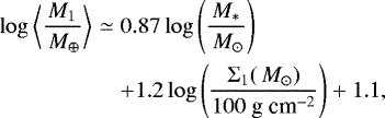
The intercept CM2, which is equal to log⟨M1∕ M⊕⟩ in 1 M⊙ models, is well expressed by Σ1 and can be given by
 (6)
(6)
This surface density dependence is almost identical to one in Kokubo et al. (2006), where the surface density dependence of the largest planet mass is 1.1log(Σ1∕10 g cm−2) + 0.079. The most massive planets in our M* = M⊙ models havesmaller masses than those in Kokubo et al. (2006), who considered the giant impact growth of planets around 1 au. This is because collisions are more effective than scattering and several (4.8–9.3) smaller planets of a similar mass form in close-in orbits while a few (≲4) larger planets form around 1 au (Matsumoto et al. 2015; Matsumoto & Kokubo 2017). This can also be interpreted by eesc, which is an increasing function of the semimajor axis. The eesc values in Kokubo et al. (2006) are about 0.3. As eesc increases, the mass of the most massive planets increases due to strong scattering.
The number of the final planets in the collision-dominated regime is also well expressed by the power-law function of Σ1,
 (7)
(7)
The number of the final planets can be determined by the relation between the total mass (∝ Σ1) and the most massive planets ( , Eq. (6)) based on mass conservation in the collision-dominated regime.
We derived CM3 from Eq. (5) with ⟨M1⟩ = Mej and log⟨M1∕ M⊕⟩ directly from our results. These values are almost the same. In the ejection-dominated regime,
 (8)
(8)
The dependence of log⟨M1∕ M⊕⟩ on the surface density in this regime becomes slightly weaker than one in the collision-dominated regime. For a given Σ1, the mass of the most massive planets in the ejection-dominated regime corresponds to the intersection point between ⟨M1 ⟩ in the collision-dominated regime and Mej. As Σ1 decreases, this point shifts toward the lower mass stars (Eq. (4), Fig. 3). This makes the dependence of log ⟨M1∕ M⊕⟩ on Σ1 slightly weaker than CM2. We also derived Cn3 and log⟨nlast⟩,
 (9)
(9)
which has a similar dependence as in Kokubo et al. (2006).
While Cn3 is within 1σ values of log ⟨nlast⟩, the number of the final planets in the Σ1 = 100 g cm−2 case is overestimated (see points and fitting line of Σ1 = 100 g cm−2 models in Fig. 3). In these models, most of the initial protoplanets have larger masses than the ejection mass. Ejections frequently occur and the number of planets becomes small. These features can be confirmed by the results of models Ms5Σ100b8 and Ms5Σ100b6, where the initial protoplanets are less massive than those in the Ms5Σ100b10 model. The numbers of the final planets are slightly larger than in the Ms5Σ100b10 model since ejection becomes less effective. This suggests that planets only grow via a few collisions and these collisions determine the final planetary mass in the ejection-dominated regime. This implies that the growth of protoplanets would be stalled at the ejection mass if the masses of the initial protoplanets are smaller than the ejection mass.
We determined the dependencies of M1, which are proportional to  in the collision-dominated regime and Σ1 in the ejection-dominated regime. These dependencies are different from that of the isolation mass, which is proportional to
  . Moreover, the ejection mass would set the upper limit of M1 when protoplanetsare less massive than Mej. These reflect the dynamical process in the giant impact growth.
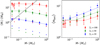 |
Fig. 3 Average values of the most massive planets (⟨M1⟩) and the number of planets (⟨nlast⟩) in a system are shown as a function of the stellar mass. The length of the error bars is equal to the standard deviation. We plotted the results of Σ1 = 10 g cm−2 in blue filled symbols, Σ1 = 30 g cm−2 in green filled ones, and Σ1 = 100 g cm−2 in red filled ones. The open circles are the results of models Ms5Σ100b8 (left) and Ms5Σ100b6 (right), which are plotted at slightly large M* to avoid overlapping. Left panel: dashed line is the ejection mass (Mej) given by Eq". (4). The triangles are the mass of the largest and smallest initial protoplanets. The dotted lines are the fitting lines. In the collision-dominated regime (⟨M1 ⟩ < Mej), we derived the fitting lines from the mass of the most massive planets and the final number of planets in all of the simulation results. In the ejection-dominated regime (⟨M1 ⟩ > Mej), these lines are constant and equal to those values at ⟨M1⟩ = Mej. |
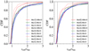 |
Fig. 4 Cumulative distribution of the collision velocities normalized by the escape velocity. Vertical black-dotted lines are vcol = vesc and vcol = 2vesc. |
3.3 Collision velocities
While we assume the perfect accretion, collisional outcomes depend on collision velocities. The cumulative distributions of the collision velocities are shown in Fig. 4. In most of the models, these distributions are similar. In the Ms0Σ100b10 and Ms1Σ100b10 models, the average collision velocities that are normalized by the escape velocities (vcol∕vesc) are 1.37 ± 0.60 and 1.31± 0.53, respectively. In the Σ1 = 100 g cm−2 models, the collision velocities become lower as the stellar mass decreases. While high vcol ∕vesc collisions occur when protoplanets experience some close scattering events before collisions, protoplanets are ejected after a few close scattering events in the ejection-dominated regime. Thus, high velocity collisions occur less frequently in the ejection-dominated regime. This is why the distribution of the collision velocities fall primarily on the small value around low-mass stars.
Most of the collisions in our simulations do not cause erosion, but perfect accretion, partial accretion, graze-and-merge, and hit-and-run (Asphaug 2010; Leinhardt & Stewart 2012; Stewart & Leinhardt 2012). The properties of collisions in our simulations are similar to the previous studies that consider N-body simulations with realistic collisions around stars of 1 solar mass (Kokubo & Genda 2010; Chambers 2013; Poon et al. 2020). These studies find that there are no substantial differences from simulations with only perfect accretion. This is because the energy dissipation in hit-and-run collisions induces another collision that leads to accretion (Emsenhuber & Asphaug 2019a,b). Our results do not change significantly if we consider these realistic collisions.
3.4 Distribution of planets around M dwarfs
3.4.1 Mass relation between massive super-Earths and stars
We investigate the observable planets using a certain relation between the surface density and the stellar mass. The dependence of the surface density of protoplanets on the stellar mass ( ) is not known. We adopt hd = 1 according to the recent study about the surface density of observed planets (Dai et al. 2020, hd = 1.04). This dependence is also adopted in the fiducial case of Raymond et al. (2007) and slightly shallower than that of the protoplanetary mass formed via pebble accretion (Liu et al. 2019, hd = 4∕3). Under this dependence, we consider two series of models. Models Ms1Σ100b10, Ms3Σ30b10, and Ms5Σ10b10 correspond to Σ1 ≃ 100 g cm−2(M*∕10−1∕4 M⊙), and models Ms0Σ100b10, Ms2Σ30b10, and Ms4Σ10b10 correspond to Σ1 ≃ 100 g cm−2(M*∕ M⊙). We refer to the former series as the massive series and the latter series as the less-massive series.
These series reproduce the mass distribution of the observed massive super-Earths well (Fig. 1). In the massive series, the mass of the most massive planets is estimated to be 22 M⊕ around 1 M⊙ stars and 3.0 M⊕ around 0.1 M⊙ stars (Sect. 3.2, Eq. (10)). These masses are in agreement with the typical mass of the observed massive super-Earths (e.g., Butler et al. 2006; Anglada-Escudé et al. 2016; Gillon et al. 2017; Zechmeister et al. 2019). We note that we focus on the distribution of massive super-Earths, which are observable around low-mass stars by ongoing and upcoming observational missions of RV measurements. The surface densities in the massive and less-massive series are similar to those estimated by RV planets and larger than those by the California-Kepler Survey (Dai et al. 2020).
3.4.2 Orbits and masses of planets
Figure 5 shows the distribution of the final planets in each series. The most massive planets form between ~ 0.1 and ~ 1 au, which correspond to the initial distribution of the protoplanets. Less massive planets are scattered and more widely distributed. The eccentricities of scattered planets are higher than the massive ones. These two groups (the massive planets and scattered planets) exhibit the bimodal distribution of planetary masses. These features can be seen in both series.
Several planets are located at ~10−2 au, while most innermost planets are located at 0.05–0.1 au, which is almost the same location of the initial innermost protoplanets. When a planet is scattered to the inner orbit by a strong scattering associated with an ejection event, a planet is pushed further into the inner orbit than the orbit of the innermost protoplanet.This dynamical process was already found in the previous studies, which considered the dynamical evolution of multiple Jupiter-sized planet systems (e.g., Marzari & Weidenschilling 2002; Nagasawa et al. 2008). Figure 5 of Nagasawa et al. (2008) showed a similar gap structure in the distribution of the semimajor axes of planets with our results.
More massive stars have more massive planets due to large surface densities (the top panels). We also show ⟨M1 ∕ M⊕⟩, which was estimated by Eq. (5) in these panels. The most massive planets are described by this equation well. By substituting Σ1 ∝ M*, CM1 ≃−1∕3 (Table 2), and CM2 (Eq. (6)) in Eq. (5), we obtain the dependence of the most massive planet on the stellar mass,
 (10)
(10)
where Σ1(M⊙) is Σ1 at M* = M⊙.
The eccentricities and inclinations of the scattered planets are expressed by eesc of the massive planets well.These eesc can be estimated by substituting Eq. (10) for Eq. (3),
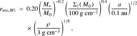 (11)
(11)
which increase as the stellar mass decreases. Table 3 summarizes eccentricities of the massive and scattered planets that are normalized by eesc,M1. In the estimation of eesc,M1, we adopted a values from the numerical results. The eccentricities of massive planets are ≲ eesc,M1 since these are damped through the giant impacts (Matsumoto et al. 2015; Matsumoto & Kokubo 2017). The eccentricities of the scattered planets are ~ eesc,M1 with the standard deviation ~eesc,M1. In the Ms0Σ100b10 model where planets form around 1 M⊙ stars, eccentricities of the massive planets are ⟨e⟩ = 0.13 ± 0.089 and those of the scattered planets are ⟨e⟩ = 0.20 ± 0.12. These eccentricities are higher than those observed by the Kepler mission (~ 0.01–0.1, e.g., Fabrycky et al. 2014; Van Eylen & Albrecht 2015; Xie et al. 2016; Van Eylen et al. 2019; Mills et al. 2019). This is because we focus on massive super-Earths (Sect. 3.4.1) and more massive planets cause stronger scattering (eesc, Eq. (3)). Moreover, planets that are located at 0.01–0.1 au and those that have high eccentricities and inclinations are affected by the stellar tide. Their eccentricities and inclinations would be damped by the tidal interaction after the giant impact stage (e.g., Goldreich & Soter 1966; Papaloizou & Terquem 2010; Papaloizou et al. 2018). We also discuss the relation between final orbital separations and eccentricities from the point of the orbital crossing timescale in Appendix A.
We consider the radial velocity of a planet larger than 1 m s−1 to be the criterion for an observable planet. We assumed sini = 1 in the estimation of the radial velocity amplitudes. The planets that satisfy this criterion are plotted as circles and those with smaller radial velocities are triangles in Fig. 5. Most of the massive planets and scattered planets located at a < 1 au in models Ms0Σ100b10 and Ms1Σ100b10 are observable. As the stellar mass decreases, only planets that are closer to their stars are observable, even if the planets have ⟨M1⟩ mass (the top panels of Fig. 5). The radial velocity amplitude of the massive planet (K1) is
 (12)
(12)
where we use Eq. (10) and M1 ≪ M*. The radial velocity amplitude of planets around low-mass stars is small since planets are less massive around low-mass stars. Unobservable planets with radial velocity amplitudes less than 1 ms−1 would exist at ≳1 au around M dwarfs.
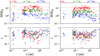 |
Fig. 5 Snapshots of the final planets plotted on the a−M (top) and a−e (bottom) planes. The planets, which are represented by circles and triangles, have larger and smaller radial velocity amplitudes than 1 m s−1, respectively. The dotted lines in the top panels are given by Eq. (5) for M1 ∕ M⊕. Left panels: we plotted the results of the massive series, which include models Ms1Σ100b10 (red symbols), Ms3Σ30b10 (green ones),and Ms5Σ10b10 (blue ones). Right panels: we plotted the results of the less-massive series, which are models Ms0Σ100b10 (red symbols), Ms2Σ30b10 (green ones),and Ms4Σ10b10 (blue ones). |
Eccentricities normalized by eesc,M1 of massive and scattered planets.
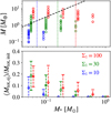 |
Fig. 6 Mass of the ejected protoplanets and the ejection rate are shown in the top and bottom panels, respectively. The stellar mass in the Σ1 = 100 g cm−2 and Σ1 = 10 g cm−2 models is plotted for slightly different M* values to easily compare the results. The dashed line in the top panel is the ejection mass (Eq. (4)). The vertical dotted lines in the top panel represent the boundary between the ejection-dominated regime and the collision-dominated regime. The error bars in the bottom panel are equal to the standard deviation. |
3.5 Ejected protoplanets
Figure 6 shows the mass of each ejected protoplanet and the ejection rate, which is given by the ratio between the total mass of the ejected protoplanets and the total initial mass. In the Σ1 = 100 g cm−2 models, the boundary between the ejection and collision-dominated regimes is located around 10−1∕2 M⊙. However, some planets are ejected when M* = 10−1∕4 M⊙ (the Ms1Σ100b10 model), which is in the collision-dominated regime. These ejections tend to occur in the outer region (≳ 1 au) where eesc is high (Eq. (3)). The same features are confirmed in the Σ1 = 30 and 10 g cm−2 models.
The masses of the ejected planets are almost in the range of the initial protoplanets (Fig. 3). In our setting, small-sized protoplanets are initially located close to the central stars. These protoplanets grow via collisions rather than scatter since their eesc is small (Eq. (3)). In contrast, the outer large protoplanets have high eesc and strongly scatter from each other. After the inner protoplanets grow via collisions, some outer protoplanets that do not grow and have their initial mass are ejected.
The ejection rate increases as M* decreases and Σ1 increases. In the ejection-dominated regime, the averaged ejection rates are ≳ 10%. For the surface density withhd = 1, planets are always ejected in the massive series with 2.2%–8.0% ejection rates. In the less-massive series, ejections occur when 10−1∕2 M⊙ and 10−1 M⊙ and the ejection rates are 1.6 and 2.3%, respectively. It is plausible that more than a few percentages of the initial mass of protoplanets are ejected from the close-in orbits of low-mass stars in the giant impact stage. These ejected planets would become free-floating planets. Free-floating planetary-mass objects are detected by the gravitational microlensing observations (e.g., Sumi et al. 2011; Mróz et al. 2017). In our results, the planets with masses ≳ 0.1 M⊕ were ejected; the averaged total mass of the ejected planets from a star was between 0.3 M⊕ and 0.9 M⊕ in the massive series and 0.09 M⊕ and 0.2 M⊕ in the less massive series. These ejected planets would be detected by future observations (Johnson et al. 2020).
4 Conclusion
Recent observations have revealed the distribution of close-in super-Earths around M dwarfs. The mass distribution of close-in super-Earths shows that small planets are orbiting around low-mass stars and ~ 10 Earth-mass planets are absent around ~0.1 M⊙ stars (Fig. 1). We have investigated the in-situ formation of close-in super-Earths via giant impacts of protoplanets around M dwarfs in a gas-free environment to explain these observed features. We performed N-body simulations while systematically changing the stellar mass and the surface density. We found that there are two regimes of planetary growth, the collision-dominated growth regime and ejection-dominated growth regime. These regimes are divided by eesc, which is calculated as the escape velocity divided by the Kepler velocity. When eesc is small, planets grow via giant impacts and their growth is in the collision-dominated regime. In this regime, the largest mass and number of final planets are well expressed by the power-law of the stellar mass and surface density. When eesc exceeds approximately 0.4, planets do not grow and some planets are ejected due to several close scattering events. This regime is the ejection-dominated regime. In this regime, the largest mass and number of final planets are almost constant. The boundary of the planet mass between these regimes is 3.0 M⊕ at 0.1 au around a 0.1 M⊙ star (Eq. (4)). This boundary mass agrees with the mass distribution of the observed close-in super-Earths around low-mass stars (Fig. 1). This suggests that the initial protoplanets are less massive than this boundary mass and their growthstalls at the boundary mass around low-mass stars.
We performed parameter surveys on the stellar mass (M*) and the surface density of the protoplanets’ (Σ1) plane and consider mass and orbital elements of observable planets via the 1 m s−1 radial velocity criterion. We employed the linear relation, Σ1 ∝ M*, to reproduce the mass distribution of observed super-Earths. We considered two series of models and show the distribution of the planets in these series of models. The mass and orbital distributions of the planets in these two series display similar trends. The massive planets grow in the range of the initial locations of protoplanets and thus they are located between ~ 0.1 and ~ 1 au. The less massive planets are scattered by the massive planets and they are also located at ≲ 0.1 au or ≳ 1 au. The planetary mass is more massive around more massive stars. In contrast, eesc of the massive planets decreases around more massive stars. The eccentricities and inclinations of the scattered planets are expressed by eesc of the massive planets. The eccentricities and inclinations of the massive ones are smaller than those of the scattered ones since their eccentricities and inclinations are damped through giant impacts (Matsumoto et al. 2015; Matsumoto & Kokubo 2017).
We found that ejections of protoplanets occur even in the collision-dominated regime. Our results suggest that ejection events occuraround late M dwarfs and a few protoplanets would be ejected from the close-in orbits around late M dwarfs.
Our results showed that Earth-mass planets around low-mass stars form via the dynamically hot evolution of protoplanets in the giant impact stage. While we do not consider planetesimals, the giant impact growth of protoplanets would be affected by planetesimals when they damp eccentricities of protoplanets. The dynamically hot evolution of protoplanets would affect the water delivery of planets by planetesimals since the ice line location is close to the central star around low-mass stars (Ida & Lin 2005; Raymond et al. 2007). The formation of Earth-mass planets around low-mass stars from planetesimals is the subject of our future work.
Acknowledgements
We thank the anonymous referee for helpful comments. This work was achieved using the grant of NAOJ Visiting Joint Research supported by the Research Coordination Committee, National Astronomical Observatory of Japan (NAOJ), National Institutes of Natural Sciences (NINS). This research was also supported by MOST in Taiwan through the grant MOST 105-2119-M-001-043-MY3. E. K. is supported by JSPS KAKENHI Grant Number 18H05438. Numerical simulations were carried out on the PC cluster at the Center for Computational Astrophysics, National Astronomical Observatory of Japan, and at the Academia Sinica Institute for Astronomy and Astrophysics (ASIAA).
Appendix A Separation–eccentricity relation
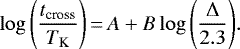
Orbital separations and eccentricities of planets affect their orbital crossing time. In this section, we investigate their relation. Zhou et al. (2007) derived an empirical formula of the orbital crossing time of planets as a function of the orbital separation and eccentricities from N-body simulations. Their formula was modified to apply to planets whose masses and orbital separations are not identical under the concept of the orbital crossing time of each planet pair by Ida & Lin (2010). This estimation of the orbital crossing time of each pair (tcross) is
 (A.1)
(A.1)
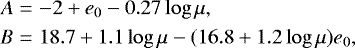
The coefficients A and B depend on the orbital separation and eccentricities. For an adjacent planet pair (i, i + 1), A and B are
 (A.2)
(A.2)
where
 (A.3)
(A.3)
We note that this estimation does not include the effect of the number of planets (Chambers et al. 1996; Funk et al. 2010; Matsumoto et al. 2012)and large dispersion of the orbital separations. Wu et al. (2019) investigated the orbital crossing time of planets whose Δ is not uniform and found that their orbital crossing time is equal or longer than the estimation using the minimum separation. This suggests that the actual crossing times are much longer than the orbital crossing time estimated by Eq. (A.1).
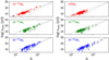 |
Fig. A.1 Orbital crossing time (tcross) of each planet pair is plotted as a function of the orbital separation in the mutual Hill radius (Δ). Left panels: results in the massive series (models Ms1Σ100b10, Ms3Σ30b10, and Ms5Σ10b10), and right: those in the less-massive series (models Ms0Σ100b10, Ms2Σ30b10, and Ms4Σ10b10), respectively. Three dotted lines are the orbital crossing time with e = 0 planets (left one), 0.5eesc,M1 planets (middle one), and eesc,M1 planets (right one) estimated by Eq. (A.1). |
We show the orbital crossing time of each adjacent planet pair in planetary systems of the massive and less-massive series (Sect. 3.4.1) as a function of Δ in Fig. A.1. We also plotted the orbital crossing time with e = 0, 0.5eesc,M1, and eesc,M1 as the dotted lines. We find that separations are concentrated in the range from Δ = 20 to 30 since the planetary system is stable for much longer than 107 yr when ≳ 20RH. Almost all orbital crossing times of the planet pairs are between the e = 0 and eesc,M1 lines. Specifically, the orbital crossing times in models 10−1∕4 M⊙ and 1 M⊙ are located above the e = 0.5eesc,M1 line. As the stellar mass decreases, more planet pairs are distributed between the e = 0.5eesc,M1 and eesc,M1 lines. These distributions arise due to their formation processes. High eesc of planets around low-mass stars make planets eccentric and their orbital separations wider.
References
- Agnor, C. B., Canup, R. M., & Levison, H. F. 1999, Icarus, 142, 219 [NASA ADS] [CrossRef] [Google Scholar]
- Andrews, S. M., Rosenfeld, K. A., Kraus, A. L., & Wilner, D. J. 2013, ApJ, 771, 129 [NASA ADS] [CrossRef] [Google Scholar]
- Angelo, I., Rowe, J. F., Howell, S. B., et al. 2017, AJ, 153, 162 [NASA ADS] [CrossRef] [Google Scholar]
- Anglada-Escudé, G., Amado, P. J., Barnes, J., et al. 2016, Nature, 536, 437 [NASA ADS] [CrossRef] [PubMed] [Google Scholar]
- Asphaug, E. 2010, Geochemistry, 70, 199 [NASA ADS] [CrossRef] [Google Scholar]
- Bonfils, X., Astudillo-Defru, N., Díaz, R., et al. 2018, A&A, 613, A25 [NASA ADS] [CrossRef] [EDP Sciences] [Google Scholar]
- Butler, R. P., Wright, J. T., Marcy, G. W., et al. 2006, ApJ, 646, 505 [NASA ADS] [CrossRef] [Google Scholar]
- Chambers, J. E. 2013, Icarus, 224, 43 [NASA ADS] [CrossRef] [Google Scholar]
- Chambers, J. E., Wetherill, G. W., & Boss, A. P. 1996, Icarus, 119, 261 [Google Scholar]
- Chiang, E., & Laughlin, G. 2013, MNRAS, 431, 3444 [Google Scholar]
- Ciesla, F. J., Mulders, G. D., Pascucci, I., & Apai, D. 2015, ApJ, 804, 9 [NASA ADS] [CrossRef] [Google Scholar]
- Dai, F., Winn, J. N., Schlaufman, K., et al. 2020, AJ, 159, 247 [Google Scholar]
- Dressing, C. D., & Charbonneau, D. 2013, ApJ, 767, 95 [NASA ADS] [CrossRef] [Google Scholar]
- Dressing, C. D., & Charbonneau, D. 2015, ApJ, 807, 45 [NASA ADS] [CrossRef] [Google Scholar]
- Emsenhuber, A., & Asphaug, E. 2019a, ApJ, 875, 95 [Google Scholar]
- Emsenhuber, A., & Asphaug, E. 2019b, ApJ, 881, 102 [Google Scholar]
- Fabrycky, D. C., Lissauer, J. J., Ragozzine, D., et al. 2014, ApJ, 790, 146 [Google Scholar]
- Funk, B., Wuchterl, G., Schwarz, R., Pilat-Lohinger, E., & Eggl, S. 2010, A&A, 516, A82 [NASA ADS] [CrossRef] [EDP Sciences] [Google Scholar]
- Gillon, M., Triaud, A. H. M. J., Demory, B.-O., et al. 2017, Nature, 542, 456 [NASA ADS] [CrossRef] [PubMed] [Google Scholar]
- Goldreich, P., & Soter, S. 1966, Icarus, 5, 375 [Google Scholar]
- Hansen, B. M. S., & Murray, N. 2012, ApJ, 751, 158 [Google Scholar]
- Hansen, B. M. S., & Murray, N. 2013, ApJ, 775, 53 [Google Scholar]
- Hardegree-Ullman, K. K., Cushing, M. C., Muirhead, P. S., & Christiansen, J. L. 2019, AJ, 158, 75 [NASA ADS] [CrossRef] [Google Scholar]
- Hayashi, C. 1981, Prog. Theor. Phys. Suppl., 70, 35 [NASA ADS] [CrossRef] [MathSciNet] [Google Scholar]
- Hirano, T., Fukui, A., Mann, A. W., et al. 2016, ApJ, 820, 41 [Google Scholar]
- Ida, S., & Lin,D. N. C. 2005, ApJ, 626, 1045 [Google Scholar]
- Ida, S., & Lin,D. N. C. 2010, ApJ, 719, 810 [Google Scholar]
- Ida, S., Muto, T., Matsumura, S., & Brasser, R. 2020, MNRAS, 494, 5666 [Google Scholar]
- Izidoro, A., Ogihara, M., Raymond, S. N., et al. 2017, MNRAS, 470, 1750 [Google Scholar]
- Izidoro, A., Bitsch, B., Raymond, S. N., et al. 2019, A&A submitted, [arXiv:1902.08772] [Google Scholar]
- Johansen, A., & Lambrechts, M. 2017, Ann. Rev. Earth Planet. Sci., 45, 359 [NASA ADS] [CrossRef] [Google Scholar]
- Johansen, A., Davies, M. B., Church, R. P., & Holmelin, V. 2012, ApJ, 758, 39 [Google Scholar]
- Johnson, J. A., Petigura, E. A., Fulton, B. J., et al. 2017, AJ, 154, 108 [Google Scholar]
- Johnson, S. A., Penny, M. T., Gaudi, B. S., et al. 2020, AJ, 160, 123 [Google Scholar]
- Kaltenegger, L., & Traub, W. A. 2009, ApJ, 698, 519 [Google Scholar]
- Kley, W., & Nelson, R. P. 2012, ARA&A, 50, 211 [Google Scholar]
- Kokubo, E., & Genda, H. 2010, ApJ, 714, L21 [Google Scholar]
- Kokubo, E., & Ida, S. 1996, Icarus, 123, 180 [Google Scholar]
- Kokubo, E., & Ida, S. 1998, Icarus, 131, 171 [Google Scholar]
- Kokubo, E., & Ida, S. 2000, Icarus, 143, 15 [Google Scholar]
- Kokubo, E., & Ida, S. 2002, ApJ, 581, 666 [Google Scholar]
- Kokubo, E., & Makino, J. 2004, PASJ, 56, 861 [Google Scholar]
- Kokubo, E., Kominami, J., & Ida, S. 2006, ApJ, 642, 1131 [Google Scholar]
- Lambrechts, M., & Johansen, A. 2012, A&A, 544, A32 [Google Scholar]
- Leinhardt, Z. M., & Richardson, D. C. 2005, ApJ, 625, 427 [Google Scholar]
- Leinhardt, Z. M., & Stewart, S. T. 2012, ApJ, 745, 79 [NASA ADS] [CrossRef] [Google Scholar]
- Lissauer, J. J. 2007, ApJ, 660, L149 [NASA ADS] [CrossRef] [Google Scholar]
- Liu, B., Lambrechts, M., Johansen, A., & Liu, F. 2019, A&A, 632, A7 [NASA ADS] [CrossRef] [EDP Sciences] [Google Scholar]
- Liu, B., Lambrechts, M., Johansen, A., Pascucci, I., & Henning, T. 2020, A&A, 638, A88 [EDP Sciences] [Google Scholar]
- Makino, J. 1991, PASJ, 43, 859 [NASA ADS] [Google Scholar]
- Makino, J., & Aarseth, S. J. 1992, PASJ, 44, 141 [NASA ADS] [Google Scholar]
- Manara, C. F., Morbidelli, A., & Guillot, T. 2018, A&A, 618, L3 [NASA ADS] [CrossRef] [EDP Sciences] [Google Scholar]
- Marzari, F., & Weidenschilling, S. J. 2002, Icarus, 156, 570 [Google Scholar]
- Matsumoto, Y., & Kokubo, E. 2017, AJ, 154, 27 [Google Scholar]
- Matsumoto, Y., & Ogihara, M. 2020, ApJ, 893, 43 [Google Scholar]
- Matsumoto, Y., Nagasawa, M., & Ida, S. 2012, Icarus, 221, 624 [Google Scholar]
- Matsumoto, Y., Nagasawa, M., & Ida, S. 2015, ApJ, 810, 106 [Google Scholar]
- Mills, S. M., Howard, A. W., Petigura, E. A., et al. 2019, AJ, 157, 198 [Google Scholar]
- Montgomery, R., & Laughlin, G. 2009, Icarus, 202, 1 [Google Scholar]
- Moriarty, J., & Ballard, S. 2016, ApJ, 832, 34 [Google Scholar]
- Mróz, P., Udalski, A., Skowron, J., et al. 2017, Nature, 548, 183 [Google Scholar]
- Nagasawa, M., Ida, S., & Bessho, T. 2008, ApJ, 678, 498 [NASA ADS] [CrossRef] [Google Scholar]
- Ogihara, M., & Hori, Y. 2020, ApJ, 892, 124 [Google Scholar]
- Ogihara, M., & Ida, S. 2009, ApJ, 699, 824 [Google Scholar]
- Ogihara, M., Morbidelli, A., & Guillot, T. 2015, A&A, 578, A36 [NASA ADS] [CrossRef] [EDP Sciences] [Google Scholar]
- Ogihara, M., Kokubo, E., Suzuki, T. K., & Morbidelli, A. 2018, A&A, 615, A63 [NASA ADS] [CrossRef] [EDP Sciences] [Google Scholar]
- Ormel, C. W., & Klahr, H. H. 2010, A&A, 520, A43 [NASA ADS] [CrossRef] [EDP Sciences] [Google Scholar]
- Papaloizou, J. C. B., & Terquem, C. 2010, MNRAS, 405, 573 [NASA ADS] [Google Scholar]
- Papaloizou, J. C. B., Szuszkiewicz, E., & Terquem, C. 2018, MNRAS, 476, 5032 [Google Scholar]
- Pfyffer, S., Alibert, Y., Benz, W., & Swoboda, D. 2015, A&A, 579, A37 [NASA ADS] [CrossRef] [EDP Sciences] [Google Scholar]
- Poon, S. T. S., Nelson, R. P., Jacobson, S. A., & Morbidelli, A. 2020, MNRAS, 491, 5595 [Google Scholar]
- Rasio, F. A., & Ford, E. B. 1996, Science, 274, 954 [NASA ADS] [CrossRef] [PubMed] [Google Scholar]
- Raymond, S. N., & Morbidelli, A. 2020, ArXiv e-prints, [arXiv:2002.05756] [Google Scholar]
- Raymond, S. N., Scalo, J., & Meadows, V. S. 2007, ApJ, 669, 606 [Google Scholar]
- Raymond, S. N., Kokubo, E., Morbidelli, A., Morishima, R., & Walsh, K. J. 2014, in Protostars and Planets VI, eds. H. Beuther, R. S. Klessen, C. P. Dullemond, & T. Henning (Tucson, AZ: University of Arizona Press), 595 [Google Scholar]
- Reid, I. N., & Hawley, S. L. 2005, New Light on Dark Stars : Red Dwarfs, Low-Mass Stars, Brown Dwarfs (Berlin: Springer) [Google Scholar]
- Rein, H. 2012, MNRAS, 427, L21 [NASA ADS] [Google Scholar]
- Safronov, V. S. 1972, Evolution of the Protoplanetary Cloud and Formation of the Earth and Planets (Israel: Israel Program for Scientific Translations) [Google Scholar]
- Stewart, S. T., & Leinhardt, Z. M. 2012, ApJ, 751, 32 [Google Scholar]
- Sumi, T., Kamiya, K., Bennett, D. P., et al. 2011, Nature, 473, 349 [Google Scholar]
- Tanaka, H., Takeuchi, T., & Ward, W. R. 2002, ApJ, 565, 1257 [NASA ADS] [CrossRef] [Google Scholar]
- Van Eylen, V., & Albrecht, S. 2015, ApJ, 808, 126 [Google Scholar]
- Van Eylen, V., Albrecht, S., Huang, X., et al. 2019, AJ, 157, 61 [Google Scholar]
- Ward, W. R. 1986, Icarus, 67, 164 [Google Scholar]
- Weiss, L. M., Isaacson, H. T., Marcy, G. W., et al. 2018a, AJ, 156, 254 [Google Scholar]
- Weiss, L. M., Marcy, G. W., Petigura, E. A., et al. 2018b, AJ, 155, 48 [Google Scholar]
- Wetherill, G. W., & Stewart, G. R. 1989, Icarus, 77, 330 [Google Scholar]
- Williams, J. P., & Cieza, L. A. 2011, ARA&A, 49, 67 [NASA ADS] [CrossRef] [Google Scholar]
- Winn, J. N., & Fabrycky, D. C. 2015, ARA&A, 53, 409 [NASA ADS] [CrossRef] [Google Scholar]
- Wu, D.-H., Zhang, R. C., Zhou, J.-L., & Steffen, J. H. 2019, MNRAS, 484, 1538 [Google Scholar]
- Xie, J.-W., Dong, S., Zhu, Z., et al. 2016, Proc. Natl. Acad. Sci., 113, 11431 [Google Scholar]
- Zechmeister, M., Dreizler, S., Ribas, I., et al. 2019, A&A, 627, A49 [NASA ADS] [EDP Sciences] [Google Scholar]
- Zhou, J.-L., Lin, D. N. C., & Sun, Y.-S. 2007, ApJ, 666, 423 [Google Scholar]
All Tables
All Figures
|
Fig. 1 Distribution of observed planets on the stellar mass in the solar mass unit (M* [M⊙]) and planetary mass in the Earth mass unit (M [M⊕]) plane. The data were extracted from the NASA exoplanet archive (https://exoplanetarchive.ipac.caltech.edu/) as of April 2020. Point colors represent the semimajor axis of each planet. Planets shown in circles were detected by the radial velocity (RV) method and those in triangles were detected using the transit or transit timing methods. The dashed line is the ejection mass at 0.1 au, given by Eq. (4). |
| In the text | |
|
Fig. 2 Typical time evolution is shown for models Ms0Σ100b10 (left, M* = 1 M⊙) and Ms5Σ100b10 (right, M* = 10−5∕4 M⊙). The solid and dashed curves in the same color show the semimajor axis as well as pericenter and apocenter distances of each body. When two protoplanets collide, the merged body has the same color as that of the massive protoplanet. |
| In the text | |
|
Fig. 3 Average values of the most massive planets (⟨M1⟩) and the number of planets (⟨nlast⟩) in a system are shown as a function of the stellar mass. The length of the error bars is equal to the standard deviation. We plotted the results of Σ1 = 10 g cm−2 in blue filled symbols, Σ1 = 30 g cm−2 in green filled ones, and Σ1 = 100 g cm−2 in red filled ones. The open circles are the results of models Ms5Σ100b8 (left) and Ms5Σ100b6 (right), which are plotted at slightly large M* to avoid overlapping. Left panel: dashed line is the ejection mass (Mej) given by Eq". (4). The triangles are the mass of the largest and smallest initial protoplanets. The dotted lines are the fitting lines. In the collision-dominated regime (⟨M1 ⟩ < Mej), we derived the fitting lines from the mass of the most massive planets and the final number of planets in all of the simulation results. In the ejection-dominated regime (⟨M1 ⟩ > Mej), these lines are constant and equal to those values at ⟨M1⟩ = Mej. |
| In the text | |
|
Fig. 4 Cumulative distribution of the collision velocities normalized by the escape velocity. Vertical black-dotted lines are vcol = vesc and vcol = 2vesc. |
| In the text | |
|
Fig. 5 Snapshots of the final planets plotted on the a−M (top) and a−e (bottom) planes. The planets, which are represented by circles and triangles, have larger and smaller radial velocity amplitudes than 1 m s−1, respectively. The dotted lines in the top panels are given by Eq. (5) for M1 ∕ M⊕. Left panels: we plotted the results of the massive series, which include models Ms1Σ100b10 (red symbols), Ms3Σ30b10 (green ones),and Ms5Σ10b10 (blue ones). Right panels: we plotted the results of the less-massive series, which are models Ms0Σ100b10 (red symbols), Ms2Σ30b10 (green ones),and Ms4Σ10b10 (blue ones). |
| In the text | |
|
Fig. 6 Mass of the ejected protoplanets and the ejection rate are shown in the top and bottom panels, respectively. The stellar mass in the Σ1 = 100 g cm−2 and Σ1 = 10 g cm−2 models is plotted for slightly different M* values to easily compare the results. The dashed line in the top panel is the ejection mass (Eq. (4)). The vertical dotted lines in the top panel represent the boundary between the ejection-dominated regime and the collision-dominated regime. The error bars in the bottom panel are equal to the standard deviation. |
| In the text | |
|
Fig. A.1 Orbital crossing time (tcross) of each planet pair is plotted as a function of the orbital separation in the mutual Hill radius (Δ). Left panels: results in the massive series (models Ms1Σ100b10, Ms3Σ30b10, and Ms5Σ10b10), and right: those in the less-massive series (models Ms0Σ100b10, Ms2Σ30b10, and Ms4Σ10b10), respectively. Three dotted lines are the orbital crossing time with e = 0 planets (left one), 0.5eesc,M1 planets (middle one), and eesc,M1 planets (right one) estimated by Eq. (A.1). |
| In the text | |
Current usage metrics show cumulative count of Article Views (full-text article views including HTML views, PDF and ePub downloads, according to the available data) and Abstracts Views on Vision4Press platform.
Data correspond to usage on the plateform after 2015. The current usage metrics is available 48-96 hours after online publication and is updated daily on week days.
Initial download of the metrics may take a while.