| Issue |
A&A
Volume 641, September 2020
|
|
|---|---|---|
| Article Number | A61 | |
| Number of page(s) | 15 | |
| Section | Extragalactic astronomy | |
| DOI | https://doi.org/10.1051/0004-6361/202038265 | |
| Published online | 09 September 2020 | |
High-latitude emission from the structured jet of γ-ray bursts observed off-axis
1
INAF – Osservatorio Astronomico di Brera, Via Bianchi 46, 23807 Merate, Italy
e-mail: This email address is being protected from spambots. You need JavaScript enabled to view it.
2
Gran Sasso Science Institute, Viale F. Crispi 7, 67100 L’Aquila, AQ, Italy
3
INFN – Laboratori Nazionali del Gran Sasso, 67100 L’Aquila, AQ, Italy
4
INAF – Osservatorio Astronomico d’Abruzzo, Via M. Maggini snc, 64100 Teramo, Italy
5
INFN – Sezione di Milano-Bicocca, Piazza della Scienza 3, 20126 Milano, Italy
Received:
25
April
2020
Accepted:
16
July
2020
Abstract
The X-ray emission of γ-ray burst (GRBs) is often characterized by an initial steep decay followed by a nearly constant emission phase (so-called “plateau”) which can extend up to thousands of seconds. While the steep decay is usually interpreted as the tail of the prompt γ-ray flash, the long-lasting plateau is commonly associated to the emission from the external shock sustained by energy injection from a long-lasting central engine. A recent study proposed an alternative interpretation, ascribing both the steep decay and the plateau to high-latitude emission (HLE) from a “structured jet” whose energy and bulk Lorentz factor depend on the angular distance from the jet symmetry axis. In this work we expand on this idea and explore more realistic conditions: (a) the finite duration of the prompt emission, (b) the angular dependence of the optical depth, and (c) the dependence of the light curve on the observer viewing angle. We find that, when viewed highly off-axis, the structured jet HLE light curve is smoothly decaying with no clear distinction between the steep and flat phases, as opposed to the on-axis case. For a realistic choice of physical parameters, the effects of a latitude-dependent Thomson opacity and finite duration of the emission have a marginal effect on the overall light-curve evolution. We discuss the possible HLE of GW170817, showing that the emission would have faded away long before the first Swift-XRT observations. Finally, we discuss the prospects for the detection of HLE from off-axis GRBs by present and future wide-field X-ray telescopes and X-ray surveys, such as eROSITA and the mission concept THESEUS.
Key words: gamma-ray burst: general / relativistic processes / gravitational waves
© ESO 2020
1. Introduction
The observed prompt emission in the keV–MeV range and the multi-wavelength afterglow clearly indicate that γ-ray bursts (GRBs) originate in highly relativistic, collimated jets (see e.g., Piran 2004 and Kumar & Zhang 2015 for reviews).
At lower energies, the early light curve of GRBs shows complex behavior (e.g., Tagliaferri et al. 2005; Nousek et al. 2006; Zhang et al. 2006; O’Brien et al. 2006; Liang et al. 2007; Willingale et al. 2007): frequently, the optical and X-ray emission present different temporal decays and, more often, the X-ray light curve presents a steep decay followed by a plateau, while the optical emission is consistent with a smooth decay (e.g., Fan & Piran 2006; Panaitescu 2008; Ghisellini et al. 2007; Liang et al. 2008; Panaitescu & Vestrand 2011; Oates et al. 2011; De Pasquale et al. 2011; Zaninoni et al. 2013; Melandri et al. 2014; Li et al. 2015). The origin of the plateau is a long-standing problem of GRB physics, whose standard interpretation invokes the presence of a central engine with long-lasting activity, such as a millisecond magnetar formed after a binary neutron star merger or a stellar collapse (Dai & Lu 1998a,b; Dai 2004; Zhang & Mészáros 2001; Yu et al. 2010; Metzger et al. 2011; Dall’Osso et al. 2011).
Both the internal and external dissipation mechanisms of the jet’s kinetic energy are expected to contribute to the diversity of the observed X-ray and optical emission (e.g., see Li et al. 2015). A model including internal and external jet dissipation is required to explain the chromatic nature of the X-ray and optical light curves (e.g., plateau in X-rays and normal decay in optical bands; see e.g., Fan & Piran 2006; Oganesyan et al. 2020) the different post-plateau phases (including rarely observed fast decay; see e.g., Sarin et al. 2020), and the claimed correlations between the observed plateau and prompt emission properties (e.g., Dainotti et al. 2008; Margutti et al. 2013; Izzo et al. 2015; Tang et al. 2019).
Oganesyan et al. (2020) and Beniamini et al. (2020a) showed that a structured jet could provide an alternative explanation for the origin of the X-ray plateau in GRBs. A structured jet is an outflow where velocity and energy vary (decreasing, in general) with the angle measured from the jet axis, as opposed to a top-hat jet where these quantities are uniform within the jet opening angle. Oganesyan et al. (2020, hereafter, O20) assume an instantaneous prompt emission pulse originating from a structured jet, showing that the regions outside the jet core can produce a long-lasting X-ray plateau for an on-axis observer.
This effect is produced by the high-latitude emission (HLE), that is, the emission produced at large angles with respect to the jet axis, where the difference in the time of flight of photons (with respect to photons emitted from the axis) is high enough1 to shape the light curve in the observer frame. While HLE has already been considered to explain the tails of the prompt emission pulses (Fenimore et al. 1996), the X-ray steep-decay phase (Kumar & Panaitescu 2000; Zhang et al. 2006; Liang et al. 2007), and the tails of the X-ray flares (Jia et al. 2016), its role in producing the X-ray plateau is a novelty that was introduced for the first time in the O20 model2. A particular feature of this model is that the duration of the plateau phase increases with the distance from the central engine where the emission happens. For an appropriate combination of parameters, O20 showed that plateaus as long as a few 104 s can be produced.
Alternatively, Beniamini et al. (2020a) showed that the plateau emission can be interpreted as the external shock (afterglow) emission of a structured jet observed slightly off-axis. It is worth noting that both Beniamini et al. (2020a) and O20 models have the great advantage of being agnostic on the nature of the γ-ray burst central engine.
The idea that GRB jets are structured is supported by several theoretical studies that investigated how the jet propagates through the envelope of the massive stellar progenitor in long GRBs or through the ejecta resulting from the merger of the compact binary progenitor in short GRBs (e.g., Aloy et al. 2000, 2005; Ramirez-Ruiz et al. 2002; Matzner 2003; Zhang et al. 2003; Lazzati & Begelman 2005; Morsony et al. 2007; Bromberg et al. 2011; Lazzati & Perna 2019; Xie & MacFadyen 2019; Salafia et al. 2020). These studies showed that the jet-envelope –ejecta interaction leaves an imprint on the jet, leading to the formation of a wide angular structure.
The recent joint discovery of the gravitational-wave (GW) signal from the binary neutron star (BNS) merger GW170817, of the accompanying faint short GRB 170817A (Abbott et al. 2017a,b), and in particular, of its multi-wavelength long-lasting emission, has provided strong support to the structured jet scenario (e.g., Lazzati et al. 2018; D’Avanzo et al. 2018; Mooley et al. 2018a; Resmi et al. 2018; Lyman et al. 2018; Margutti et al. 2018; Troja et al. 2018; Ghirlanda et al. 2019; Lamb et al. 2019; Hajela et al. 2019; Salafia et al. 2019; Ioka & Nakamura 2019).
Here we aim to generalize the O20 model by relaxing some of its basic assumptions, which are: (i) the coincidence of the line of sight with the jet axis (on-axis observer), (ii) the infinitesimal duration of the energy release by the emitting surface, and (iii) the negligible opacity of the emitting region. We generalize the model, considering: a generic viewing angle with respect to the jet axis, a finite duration in the energy release, and a non-negligible opacity and its angular dependence along the emitting surface.
Moreover, the off-axis view of the γ-ray burst prompt HLE may reveal a new promising class of X-ray counterparts of GW from compact binary mergers, which add up to the already explored orphan afterglows from the external shock, cocoon emission (see Lazzati et al. 2017a,b), and spindown–powered transients (Yu et al. 2013; Metzger & Piro 2014; Siegel & Ciolfi 2016a,b; for more details on electromagnetic counterparts from GWs see Nakar 2019).
The HLEs could become a detectable target in the near future thanks to the advent of sensitive large-field-of-view surveys such as eROSITA (Merloni et al. 2012), Einstein Probe (Yuan et al. 2015), eXTP (Hernanz et al. 2018), the mission concept THESEUS-Soft X-ray Imager (SXI; Amati et al. 2018), and SVOM-ECLAIRs (Wei et al. 2016) in the X-rays. Therefore, their modelling is of great importance in order to plan observational strategies for the follow-up of GW events detected by the current and next-generation GW detectors (Abernathy 2011; Maggiore et al. 2020; Reitze et al. 2019), and to optimize the operations and development of wide-field X-ray instruments (Amati et al. 2018; Hernanz et al. 2018).
The paper is organized as follows: in Sect. 2 we describe the formalism adopted for the computation of the HLE from a structured jet for an observer at any viewing angle: we first develop the simplest case of instantaneous emission (Sect. 2.1) and then generalize to the case of finite-duration emission (Sect. 2.2). In Sect. 3 we derive the transparency condition to Thomson scattering as a function of the angular coordinate of the jet and discuss its impact on the observed X-ray light curve. In Sect. 4 we show our resulting X-ray light curves and discuss the detectability prospect of off-axis events by THESEUS and eROSITA. In this section, we also address the case of GW/GRB 170817. We discuss our findings in Sect. 5.
2. Method
In this section we outline the formalism for the computation of the HLE for an observer at any viewing angle (i.e., relaxing the assumption of an on-axis observer adopted in O20). We first consider (similary to O20) the case of instantaneous emission and then extend the treatment to the more realistic case of a pulse of finite duration. Finally, we also include the effect of a non-negligible opacity.
2.1. Instantaneous emission
Following O20 we start by assuming that all the energy is released instantaneously at the emission time 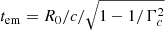 . Here R0 is the distance from the central engine along the jet axis (θ = 0) at the time when the energy is released and Γc is the bulk Lorentz factor of the core of the structured jet.
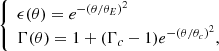
We consider two possible jet structures, which describe how the energy and the bulk Lorentz factor change as a function of the angle from the jet axis. These were first proposed in models for the afterglow emission (power-law structured jet Rossi et al. 2002; Gaussian structured jet Zhang & Mészáros 2002). The power-law structure is defined as
![Mathematical equation: $$ \begin{aligned} {\left\{ \begin{array}{ll} \epsilon (\theta ) = \Bigl [1+\Bigl (\frac{\theta }{\theta _E}\Bigr )^k\Bigr ]^{-1}\\ \Gamma (\theta ) = 1 + (\Gamma _c -1)\Bigl [1 + \Bigl (\frac{\theta }{\theta _c}\Bigr )^k\Bigr ]^{-1}. \end{array}\right.} \end{aligned} $$](/articles/aa/full_html/2020/09/aa38265-20/aa38265-20-eq2.gif) (1)
(1)
The Gaussian structure is defined as
 (2)
(2)
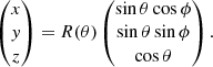
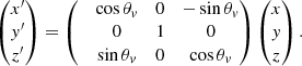
where θE and θc are the core opening angles of the (normalized) energy and Lorentz factor structure, respectively, and Γc is the bulk Lorentz factor of the core3. In order to explore how the HLE from the structured jet γ-ray burst prompt emission appears under different viewing angles, we consider two different Cartesian coordinate systems 𝒦 and 𝒦′ represented in Fig. 1 (black and blue axes, respectively). The z-axis of the 𝒦 system is aligned with the symmetry axis of the jet, while the 𝒦′ system is rotated by an angle θv (the viewing angle) around the y axis such that the axis z′ coincides with the line of sight4. Both systems are centered on and at rest with respect to the central engine, namely they are center-of-explosion (CoE) frames.
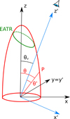 |
Fig. 1. Pictorial representation of the system under study. The emitting surface is shown in red, the reference frame 𝒦 is in black, and the frame 𝒦′, with its z′ axis aligned with the line of sight, is represented in blue. The green circle shows an example of EATR. |
At a given observer time tobs, the observer receives radiation emitted by those points of the emitting surface sharing the same value of z′. Such points define a curve on the emitting surface called the equal arrival time ring (EATR), which is described as (see Appendix A):
 (3)
(3)
where R(θ)≡β(θ)ctem is the radius at a given θ that defines the surface of emission, β(θ) the jet velocity in units of c, and tem denotes the time at which the emission occurs (all the times are measured starting from the jet launching time).
The flux at a given tobs is obtained by integrating the flux element along the EATR corresponding to a given tobs, taking into account also the Doppler factor of the emitting element. For an off-axis observer, the break of the symmetry introduces a dependence on the angle ϕ into the Doppler factor, such that it writes:
![Mathematical equation: $$ \begin{aligned} D(\theta , \phi ) = \frac{1}{\Gamma (\theta )[1-\beta (\theta )(\cos \theta \cos \theta _{ v} + \sin \theta \sin \theta _{ v}\cos \phi )]}, \end{aligned} $$](/articles/aa/full_html/2020/09/aa38265-20/aa38265-20-eq5.gif) (4)
(4)
where cos θ cos θv + sin θ sin θv cos ϕ = cos θ′ and θ′(θ, ϕ) is the polar angle of the point P in the 𝒦′ (see Fig. 1 and Appendix A). It is worth noting that, while in the on-axis case the Doppler factor depends only on θ (e.g., see O20), for an off-axis observer, the break of the symmetry introduces a further dependence on the angle ϕ.
The flux density thus can be written as:
![Mathematical equation: $$ \begin{aligned}&F_\nu (t_{\rm obs}) = \frac{1}{\mathrm{d}^2_L(1+z)^3} \nonumber \\&\qquad \ \ \times \oint _{EATR} \frac{{\eta ^{\prime }}_{\nu ^{\prime } }[\nu (1+z)/D(\theta , \phi ), \theta ]D^{3}(\theta , \phi )P(\theta , \phi , \tau )\mathrm{d}l}{|\nabla {h}(\theta , \phi )|}, \end{aligned} $$](/articles/aa/full_html/2020/09/aa38265-20/aa38265-20-eq6.gif) (5)
(5)
where z is the source redshift, ν(1 + z)/D(θ, ϕ) = ν′ is the frequency in the emitting element comoving frame,  is the emitted energy per unit area per unit frequency per unit solid angle and can be expressed as
 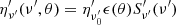 , where ϵ(θ) is the structure in energy,
  is the spectral shape normalized to 1 at
  , and the constant
  . In Eq. (5), dL is the source luminosity distance5, P(θ, ϕ, τ) is the optical depth-dependent projection factor (with τ being the optical depth) taking into account the orientation of the emitting surface with respect to the line of sight in the optically thick regime (P(θ, ϕ, τ) = 1 when the opacity is negligible), and the function h(θ, ϕ) is defined as
 (6)
(6)
such that:
![Mathematical equation: $$ \begin{aligned}&|\nabla h(\theta , \phi )| = \frac{D(\theta , \phi )\Gamma (\theta )}{c}\left\{ \frac{1}{(\partial _\theta R)^2 \,+ R^2}\bigl [\partial _\theta R\right.\nonumber \\&\qquad \qquad \quad \times (\cos \theta _{ v} \cos \theta +\sin \theta _{ v} \sin \theta )\nonumber \\&\qquad \qquad \quad + R(\cos \theta \cos \phi \sin \theta _{ v} - \cos \theta _{ v} \sin \theta )\bigr ]^2\nonumber \\&\qquad \qquad \quad \left.+ \sin ^2\theta _{ v} \sin ^2 \phi \right\} ^{1/2}. \end{aligned} $$](/articles/aa/full_html/2020/09/aa38265-20/aa38265-20-eq13.gif) (7)
(7)
Equations (4) and (5) are derived in Appendix A and Appendix B.1, respectively. Throughout the paper, we assume a smoothly broken power law (SBPL) spectral shape, expressed by the function:
 (8)
(8)
where αs and βs are the spectral indices and  is the maximum frequency of
  in the comoving frame, which corresponds in the observer frame to the on-axis maximum frequency
  . A unique comoving-frame spectrum along the jet structure is assumed. We briefly discuss the impact of this assumption on the spectral evolution observed during the steep-plateau phases in Sect. 5, while we refer the reader to Salafia et al. (2015) for a study of the consistency of the structured jet model with the Amati and Yonetoku correlations.
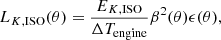
Figure 2 shows the light curve (bottom panels) for three different values of the viewing angle θv (from left to right): on-axis (θv = 0), edge of the jet core (θv = θc), and off axis (θv = 3 × θc). For these examples we considered a Gaussian jet with the following parameters: Γc = 100, R0 = 1015 cm, θc = θE = 3°, while for the spectrum we choose a SBPL function with a peak in the observer frame in the on-axis case at hνpeak = 100 keV (where h is the Planck constant) and energy spectral indices αs = 0.2, βs = 1.3, below and above the peak, respectively.
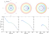 |
Fig. 2. Equal arrival time rings (top panels) and corresponding light curves (bottom panels) for three configurations of the viewing angle (from left to right), θv = 0° (on-axis), θv = θc (edge-of-the-core), and θv = 3 × θc (off-axis). Top panels: polar plot of the emitting surface. The black circle shows the physical limit of the core of the jet. The black cross shows the observer line of sight. The colored curves are the EATRs at ten arbitrary sampling times. Bottom panels: light curve normalized at its maximum value (corresponding to the on-axis observer at the first sampled epoch). The colored dots represent the flux emitted by the corresponding colored EATRs in the top panel. The structured jet assumed for this test case has a Gaussian structure with Γc = 100, θc = θE = 3°, R0 = 1015 cm. The comoving emission spectrum is described by a SBPL spectrum with αs = 0.2 and βs = 1.3. |
The upper panels in Fig. 2 show the emitting surface in polar coordinates such that the center represents the jet axis. The cross represents the position of the line of sight and the black circle marks the jet core boundary θc (which coincides with θE in the particular example shown here). The colored curves represent the EATR at different times. We note that for an on-axis observer (upper left panel) the EATRs are concentric circles, as expected from axisymmetry, while for off-axis observers (upper central and right panels) the EATRs become more and more distorted as θv increases, due to the breaking of axial symmetry combined with the latitudinal structure of the jet.
The bottom rows of Fig. 2 show the light curves, that is, the flux density Fν(t) at hν = 10 keV normalized to the maximum value received by an on-axis observer as a function of time.
In the case of an on-axis observer, shown in the left top and bottom panels of Fig. 2, the initial (from 0 to ∼50 s) steep decay of the light curve corresponds to emission produced within the core of the jet (as predicted by the analytical solution of Kumar & Panaitescu 2000). The following plateau phase (from ∼50 to ∼300 s) is instead due to photons emitted by regions just outside of the jet core: these photons are seen by the on-axis observer due to the increasing opening angles of the beaming cones in these regions characterized by a decreasing Γ.
The transition between the steep decay and the plateau phase becomes less evident as the line of sight moves to larger off-axis angles (central and right column plots of Fig. 2). For θv = θc (central column), after the peak a transition from a steep to a shallower decay can still be seen, although much less evident than in the on-axis configuration. From the top central and right panels of Fig. 2 one can see that, similarly to the on-axis case, the steep decay is produced by the emission from EATRs lying (at least partially) inside the core of the jet. The plateau is produced by EATRs just outside the core of the jet. Figure 2 shows that by increasing the viewing angle (i.e., more off-axis lines of sight) the distinction between the steep decay and the plateau sections of the light curve becomes progressively less marked.
Another feature of the off-axis light curves is the fainter peak flux density (e.g., two and four orders of magnitude for θv = θc and θv = 3θc, respectively) with respect to that measured by the on-axis observer. This effect is due to the fact that, for θv = θc and θv = 3θc, the core of the jet where ϵ(θ) and Γ(θ) reach their maximum values is beamed outside of the line of sight.
Finally, the time of arrival of the first photon is delayed for increasing viewing angle, such that for θv = 0 ° ,θc, 3θc it arrives respectively at ∼ 2 s, 10 s, and 200 s after the jet launch time.
2.2. Finite-duration emission
In the previous section, similarly to O20, we considered the simplifying assumption of an impulsive emission episode in computing its HLE light curve. In this section we generalize our calculation to the case of a finite time interval during which the energy is released. To this aim we approximate the emission episode with a temporal profile Iν(t) which is the sum of N infinitesimal pulses. Each infinitesimal pulse is treated as in the impulsive approximation. The N pulses are then summed in such a way that the total emitted energy is conserved (a more detailed description of the method is provided in Appendix B.2).
Figure 3 shows the light curve obtained with the finite-duration emission case for an on-axis observer. Also, for this example we consider a Gaussian jet with a core half-opening angle θc = θE = 3° and Γc = 100. The emission starts at a radius R0 = 1013 cm and its temporal profile is described by a step function sampled N = 105 times and lasting ΔT = 105 s in the CoE frame, which corresponds to  in the observer frame.
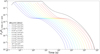 |
Fig. 3. Light curve for finite-duration emission. The case refers to an on-axis observer. The dashed colored light curves corresponding to n = 13 selected infinitesimal pulses out of the total N = 105 composing the finite-duration emission episode. Partial fluxes have been multiplied by a factor N/n in order to better visualize the contribution to the final emission at different radii. Colors identify the ΔR0, i (Δt) with respect to the initial R0 (tem) at which the first pulse is emitted. The black solid line is the final light curve made by the sum of the partial ones. We assume a Gaussian jet with parameters Γc = 100, θc = θE = 3°, R0 = 1013 cm and the pulse duration in the CoE frame ΔT = 105 s. A SBPL spectrum with αs = 0.2 and βs = 1.3 is assumed. |
In Fig. 3 the black solid line represents the total flux density, while the dashed colored lines show the contributions to the emission of the N discrete pulses, which henceforth we refer to as partial light curves6. The emitting surfaces of all pulses have the same structure but they correspond to different emission radii. We labeled each surface with the parameter ΔR0 ≡ Ri(θ = 0)−R0, where Ri(θ) is the radius of jet core for the i-th surface. Each emitting surface is characterized by the constant  (in Eq. (B.15)) which we assume - in this particular example - to be constant with time. We assume for simplicity that the spectrum and the energy profile ϵ(θ) do not change within the pulse.
We can see from Fig. 3 that also in the more realistic case of a finite-duration emission episode the light curve morphology is preserved in the on-axis case because the total light curve is dominated by the very late partial light curves. The presence of the steep decay-plateau structure in the on-axis case found by O20 is confirmed when a more realistic finite-duration emission is considered. We verified that also in the off-axis case the final partial light curves shape the total emission for most of the time, with the exception (as in the on-axis case) of the first phase, when the contribution of the early time emission is non-negligible.
It is quite important to notice – as shown in Fig. 3 – that from our model the duration of the plateau is not necessarily determined by the radius of the prompt emission. The only requirement to have a long lasting plateau is that the portion of the jet outside of the core, and not necessarily the entire surface, is emitting at large radii. We can have a scenario in which the prompt emission is generated at small radii (e.g., 1013 cm) by the core of the jet, but while the core switches off, the portion of the surface outside the core is still emitting (or it switches on and off with a delay with respect to the core) when the outflow has reached a larger distance (e.g., 1015 cm). This scenario could in principle accommodate a rapid variability of the prompt emission together with a long-lasting plateau without invoking mini jets (Kumar & Piran 2000).
3. Opacity
O20 assumed the entire emission region to be transparent. This assumption is allowed when the emission radius R0 is large. Since a large radius is also required in order to have a long-lasting plateau, this justifies the O20 approximation. Here we consider a more realistic scenario, where the effect of the latitude-dependent opacity, its variation with the radius, and the finite duration emission are included.
It is well known that ultra-relativistic motion is required in GRBs to solve the so-called compactness problem (Ruderman et al. 1975; Schmidt 1978). Originally, this argument was applied considering the main source of opacity for high-energy photons, i.e., pair production (Piran 1999; Lithwick & Sari 2001). Recently, it was also applied to constrain the viewing angle (Matsumoto et al. 2019). Considering that we aim to interpret the soft X-ray emission (0.1-10) keV, we consider hereafter only the Thomson scattering as the main source of opacity.
In Appendix C, we calculate the expression for the θ-dependent optical depth, which reads
![Mathematical equation: $$ \begin{aligned}&\tau (\theta ) = \frac{Y_e \sigma _T L_{K, \mathrm{ISO}}(\theta )}{4\pi m_p \beta (\theta ) [1 + \beta (\theta )]c^3\Gamma ^2(\theta )[\Gamma (\theta ) -1]}\nonumber \\&\qquad \ \ \times \,\left\{ \frac{1}{R(\theta )} - \frac{1}{[1+\beta (\theta )]\Gamma ^2(\theta )\Delta R(\theta ) + R(\theta )}\right\} , \end{aligned} $$](/articles/aa/full_html/2020/09/aa38265-20/aa38265-20-eq20.gif) (9)
(9)
where Ye is the electron fraction, σT = 6.65 × 10⁻²⁵ cm2 the Thomson scattering cross- section, mp = 1.67 × 10⁻²⁴ g the mass of the proton, LK, ISO(θ) the kinetic isotropic equivalent luminosity, ΔR(θ) = β(θ)cΔTengine is the width of the emitting region, and ΔTengine is the duration of the central engine. The kinetic luminosity profile is set by the relation dEK/dΩ ∝ β2(θ)ϵ(θ) (O20), such that we can write
 (10)
(10)
where EK, ISO is the isotropic equivalent kinetic energy. For these two parameters we take the reference values EK,ISO = 1054 erg and ΔTengine = 30 s, appropriate for long GRBs.
The optical depth of Eq. (9) multiplies the integrand in the RHS of Eq. (5) (B.13) through the multiplicative factor f(θ) = exp[−τ(θ)], which suppresses the emission in the regions where τ(θ) > 1. The absorption effect is shown in Fig. 4. The partial light curves emitted at small radii (dark blue dashed lines) are strongly absorbed due to the large opacity along most of the emission surface and particularly outside the jet core where Γ(θ) decreases with the increasing angle from the jet axis. However, the contributions to the emission produced at larger radii suffer a smaller absorption (as shown by the orange-red lines). Overall, also considering the effect of the angular dependence of the opacity, the appearance of the plateau for the structured jet parameters considered in this example is preserved.
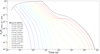 |
Fig. 4. Same as Fig. 3 but with the effect of a non-negligible and latitude-dependent opacity. The parameters for the optical depth are: Ye = 1, EK,ISO = 1054 erg and ΔTengine = 30 s. |
In the following, we restrict ourselves to the infinitesimal emission case for which we consider damping due to the opacity. This choice is motivated by the evidence that the steep decay and plateau phases mostly depend on the very late “partial” light curves (see Fig. 3), which are ascribed to the final phases of the emission of a finite pulse. However, if the emission ceases at sufficiently small radii (e.g., R0 ∼ 1014 cm) the opacity plays a dominant role in shaping the light curve (see Fig. 4) and its effect needs to be considered.
It is also worth noting that when the opacity is non-negligible, the rest-frame spectrum in the regions outside of the core is unlikely to be exactly equal to the core spectrum (due to e.g., absorption and Comptonization of photons). Despite this, for simplicity, we consider the case of a uniform unique comoving frame spectrum along the jet surface, since at large radii opacity-driven spectral corrections are expected to be negligible.
4. Results
4.1. Parametric study
Here we investigate the light-curve dependence on model parameters. We define a fiducial model by choosing a particular set of parameter values, and then vary one parameter at a time. More specifically, our fiducial model is the same adopted in Fig. 2 – namely Γc = 100, R0 = 1015 cm, θc = θE = 3° and a Gaussian structure – with a SBPL function spectrum with indices αs = 0.2 and βs = 1.3. Instead, the light curves arising from a power-law jet structure are discussed in Appendix D.
Figure 5 shows the light curves of our fiducial model (solid lines) for three values of the viewing angle θv = [0, 1, 3]×θc, which correspond to the on-axis, edge, and off-axis view and are represented in blue, orange, and green, respectively. In the same figure we report also two further models characterized by the same R0 and the same spectrum: the dashed curves are obtained by increasing the core half-opening angle (i.e., θc = θE = 5°), while the dotted curves are obtained by increasing the core Lorentz factor (i.e., Γc = 200). All the light curves are expressed as Fν(tobs) at a reference (observer frame) energy of hν = 10 keV and each curve is normalized to the maximum of the on-axis light curve. Differently from the previous figures, here the time axis refers to the time of arrival of the first photon, which, for a better visualization, we set at 10−1 s. This choice is motivated by the likely possibility that, in the upcoming years, a large fraction of off-axis GRBs will be directly detected by high-energy surveys and we will lack a reference initial time that could be provided only by a GW or neutrino trigger.
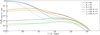 |
Fig. 5. Light curves obtained varying Γc and θc at fixed R0 = 1015 cm, at different viewing angles. Light curves corresponding to viewing angles θv = 0, θc, 3θc are shown in blue, orange, and green, respectively. Continuous curves denote the fiducial model, with Γc = 100, θc = 3°. The structure is Gaussian and the spectrum is a SBPL function with αs = 0.2 and βs = 1.3. The light curves are those at ν = 10 keV normalized to the maximum value of the on-axis case and the time is relative to the time of arrival of the first photon. For better visualization, we translated the time such that the first photons arrive at 10−1 s. |
As shown by the dotted curves in Fig. 5, the Lorentz factor of the core mainly affects the on-axis curve. A higher Lorentz factor corresponds to a steeper initial decay, and produces a bump or rebrightening at later times as the emission from outside of the core becomes dominant. Moreover, a larger Γc causes the emission to be fainter than the equivalent model with lower Γc, and in general the whole light curve fades more rapidly. This behavior can be explained by the narrower relativistic beaming of the radiation, that consequently suffers a faster angle-dependent de-beaming effect. When the EATRs cross the core boundary, the increase of the flux due to the Doppler factor overcomes the de-beaming due to the increasing latitude, producing a rebrightening instead of a plateau. The off-axis light curves instead show less prominent differences with respect to the equivalent ones in the fiducial model. The light curve corresponding to the edge-of-the-core viewing angle does not show a plateau or rebrightening. Interestingly, since the edge-of-the-core light curve shows a constant decay while the on-axis light curve has a rebrightening, under the assumption that the light curves change smoothly with θv, we may conclude that there must exist a set of θv values included in the interval (0, θc) for which the light curves present a plateau. This means that, at least in this case, observers with θv < θc but not perfectly aligned with the axis will see a plateau in the light curve.
Instead, an on-axis model with a wider core opening angle (dashed line of Fig. 5) is characterized by a longer lasting steep decay and a longer lasting and fainter plateau with respect to the fiducial model. When this is accompanied by a larger R0 the plateau can last as long as a few 104 s, as shown in O20. The off-axis light curves in this case are qualitatively similar to those of the other two models.
In Fig. 6 we consider the same models as in Fig. 5 but assuming a smaller emitting radius of R0 = 1014 cm. As in Fig. 5, the blue, orange, and green colors denote light curves at θv = [0, 1, 3]×θc respectively, while the continuous, dashed, and dotted lines identify different combinations of Γc and θc. The shape of the light curves changes substantially: the steep decay is present in all the cases while the plateau disappears. The only exception with a short plateau phase is with Γc = 200 (dotted line). By comparing this result with Fig. 4 we can understand that this effect is due to the opacity which completely suppresses the emission of the jet wings. If the opacity effect were ignored, the on-axis light curve would retain the steep decay-plateau structure, with a plateau of shorter duration than in the fiducial model (see e.g., Fig. 3). It is worth noting that the opacity-driven suppression of the plateau can be used to constrain the parameters entering in Eq. (9). For example, if we are confident in our knowledge of the parameters describing the jet structure (e.g., Γ(θ)) and those describing the microphysics (e.g., Ye), the presence of a plateau and its duration can determine the radius of emission R0. Off-axis light curves (θv = 3θc - green line) are strongly suppressed (note the different scale of the vertical axis in Figs. 5 and 6) because the radiation beamed towards the observer is quenched by the large opacity and the radiation from the core (less absorbed), which would suffer less absorption, is strongly de-beamed.
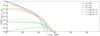 |
Fig. 6. Same as Fig. 5 but with R0 = 1014 cm. In the off-axis case (θv = 3θc) the emission is quenched as described in the text (note the different y-axis scale with respect to Fig. 5). |
4.2. Comparison with the off-axis forward shock emission
O20 modeled the X-ray and optical light curves of GRB 100906A as the sum of an on-axis HLE and afterglow (forward-shock) emission. In this work, we calculate the off-axis light curve of that model in order to investigate how the HLE and forward-shock emission compare when the source is observed off-axis. In particular, we are interested in addressing whether one of the two components dominates over the other, or the two emissions remain well separated in time. We assume the same parameters as those of the model used in O20 to describe the jet; a Gaussian structure, Γc = 160, R0 = 3 × 1015 cm and θc = 3.3° and θE = 4.4°. For the afterglow model, we consider a forward shock with ambient density n = 15 cm−3, shock-accelerated electron power-law index p = 2.1, post-shock internal energy density fraction shared by the accelerated electrons ϵe = 0.03, fraction shared by the magnetic field ϵB = 2 × 10⁻² and finally EK,ISO = 5 × 1053 erg. The off-axis forward shock model is described in Salafia et al. (2019). The spectrum of the HLE here slightly differs from the one used in O20. While O20 used a smoothed double broken power-law spectrum, here we use a simpler SBPL, with αs = 0.67, βs = 3.0 and hνpeak = 100 keV.
Figure 7 shows the corresponding HLE and the forward-shock light curves. The on-axis, edge-of-the-core, and off-axis views are represented by blue, orange, and green colors, respectively. We can see that the off-axis forward shock emission does not outshine the HLE, because it peaks when the latter has already faded. Moreover, the forward shock emission is more suppressed than the HLE for increasing viewing angles. This means that the off-axis HLE emission may be observed even when the forward shock cannot. The chosen example, GRB100906A, is a long γ-ray burst, but our results hold also for short GRBs. While short GRBs are characterized by afterglows that are fainter by a factor of approximately ten with respect to those of long GRBs (Berger 2014), a smaller factor is expected for the HLE corresponding to the difference in prompt emission luminosity of long and short GRBs (D’Avanzo et al. 2014).
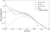 |
Fig. 7. On-axis (θv = 0 × θc), edge (θv = θc), and off-axis (θv = 3 × θc) views of HLE (continuous line) and forward shock (dashed lines) models used in O20 to fit the light curve of GRB 100906A. The light curves are integrated in the energy range 0.5 − 10 keV. HLE model parameters: Γc = 160, R0 = 3 × 1015 cm and θc = 3.3° and θE = 4.4°, spectrum: SBPL, αs = 0.67, βs = 3.0 and νpeak = 100 keV, jet structure: Gaussian. Forward shock model parameters: n = 15 cm−3, p = 2.1, ϵe = 0.03, ϵB = 2 × 10⁻², EK,ISO = 5 × 1053 erg. |
This has important implications in a multi-messenger context; for example, in the case of electromagnetic (EM) follow-up of GW from a BNS merger, the HLE emission of the associated short γ-ray burst can be detected off-axis with X-ray observations made within a few hours of the GW trigger. Furthermore, wide-field X-ray telescopes, such as eROSITA and Einstein Probe, and a mission concept such as the THESEUS-SXI could detect the off-axis HLE of long and short GRBs, irrespective of a GW trigger.
In order to illustrate the capability of these instruments to detect the off-axis HLEs, Fig. 8 shows the peak flux of our model for GRB100906A at different viewing angles by placing the source at different redshifts: z = 1.730, the actual redshift of this event, z = 0.045, corresponding to the luminosity distance of 200 Mpc, which we consider as a fiducial limit for the detection of a BNS by the LIGO and Virgo Scientific Collaborations (LVC; Abbott et al. 2018), and z = 0.5, the expected BNS range for the Einstein Telescope (ET; Abernathy 2011; Maggiore et al. 2020). The ET range corresponds to the redshift up to which 60% of the sources are expected to be detected by the interferometer (Maggiore et al. 2020). The red solid and dashed lines show the limiting fluxes of 2.6 × 10⁻¹¹ erg s−1 cm−2 (103 s of exposure time) and 10−10 erg s−1 cm−2 (102 s of exposure time) for THESEUS-SXI7 (Amati et al. 2018), respectively, while the black dashed line shows the limiting flux of 3 × 10⁻¹³ erg s−1 cm−2 (40 s of exposure time) for eROSITA (Khabibullin et al. 2012). We can see that both THESEUS and eROSITA are able to observe the HLE at the lowest z even for very large viewing angles. However, increasing the redshift reduces the viewing angle up to which an observer can detect the HLE; at z ∼ 1.730, THESEUS (100 s exposure time) and eROSITA would detect this event only if the viewing angle were smaller than ∼7° or ∼23°, respectively. Nevertheless, the larger field of THESEUS-SXI could compensate for the lower sensitivity with respect to eROSITA.
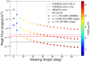 |
Fig. 8. Peak flux vs. viewing angle of the HLE of GRB 100906A assuming the same structure derived in O20. Circles, diamonds, and crosses represent the same model at three different redshifts: z = 1.730 (actual redshift of GRB 100906A), z = 0.045 (Advanced LIGO and Virgo range for BNS mergers), and z = 0.5 (ET range for BNS mergers), respectively. The color code denotes the logarithm of the time of the peak in the observer frame. Red continuous and red dashed lines mark the flux limit of THESEUS-SXI integrated in 103 s and 102 s, respectively. Black dashed line marks the flux limit of eROSITA integrated in 40 s. Verical dotted line marks θc. |
Finally, we also mention that the modeling of the forward shock is important for constraining the jet structure with the aim of robustly estimating the contribution of the HLE. In particular, Beniamini et al. (2020b) showed that, rather independently from parameters ϵB, ϵe, and n, the jet structure can be constrained from the afterglow light curves.
4.3. The Case of GW170817
The first EM signal associated with GW170817 was the faint short GRB 170817A detected by Fermi-GBM (Goldstein et al. 2017) and INTEGRAL (Savchenko et al. 2017) 1.76 s after the merger. The GRB had a peak isotropic equivalent luminosity of 1.6 × 1047 erg s−1 (Abbott et al. 2017b). No counterpart was detected by the early X-ray follow-up campaign. MAXI, the first to observe in the X-ray band at 4.8 h, provided an upper limit of 8.6 × 10⁻⁹ erg s−1 cm−2 in the energy range of (2 − 10 keV). Subsequent observations by MAXI (at 6.2, 12.0, 13.7 h) provided other limits to the X-ray flux (7.7 × 10⁻⁸, 4.2 × 10⁻⁹, 2.2 × 10⁻⁹ erg s−1 cm−2; Sugita et al. 2017; Abbott et al. 2017a). Swift observed the position of the optical counterpart AT2017gfo (Coulter et al. 2017) at 14.9 h after the merger obtaining an upper limit to the X-ray flux of 2.74 × 10⁻¹³ erg s−1 cm−2 (0.3 − 10) keV (Evans et al. 2017; Abbott et al. 2017a).
During early Chandra observations at 2.2 days after the merger, Chandra did not detect any source (Troja et al. 2017). Eventually, 8.9 days after the merger, Chandra discovered the X-ray counterpart with an estimated flux in the range (0.3 − 10) keV of (4 ± 1.1) × 10−15 erg s−1 cm−2 (Troja et al. 2017). From this date, the source emission as observed in the X-ray, optical, and radio band slowly increased with time (∝t0.8, Mooley et al. 2018b) until it peaked at ∼ 150 days after the merger (Dobie et al. 2018; D’Avanzo et al. 2018; Margutti et al. 2018). Finally, the light curve showed a rapid declining phase (Dobie et al. 2018; Alexander et al. 2018). A structured jet (Lamb et al. 2019; Margutti et al. 2018; Lazzati et al. 2018; Gottlieb et al. 2018) is able to account for the multi-wavelength light curve and the proper motion (Mooley et al. 2018a) and size constraints (Ghirlanda et al. 2019) observed in the radio band.
Here, we verify that our off-axis HLE model is consistent with the upper limits from the early X-ray observations of GW170817. To this aim, we assume the jet parameters derived from the combined modeling of the afterglow emission, source proper motion, and size constraints by Ghirlanda et al. (2019). The jet is assumed to be observed off-axis at a viewing angle θv = 15° and to have a power-law structure with core parameters Γc = 251, θc = θE = 3.4°, EK,ISO = 2.5 × 1052 erg. The angular profiles of the bulk Lorentz factor and of the energy are modeled with different power-law slopes, that is, kc = 3.5 and kE = 5.5, respectively. We consider two possible values for the emission radius R0 corresponding to R0 = 1013 cm and R0 = 2 × 1015 cm, and we model the HLE in these two limiting cases. We consider a SBPL function with hνpeak = 1500 keV ( in comoving frame), αs = 0.5, and βs = 1.3 as a reference spectrum.
Figure 9 shows the HLE emission light curve (i.e., flux integrated in the (0.3 − 10) keV energy range) for R0 = 2 × 1015 cm and R0 = 1013 cm (solid and dashed lines, respectively). The orange lines correspond to the jet seen off-axis (as it should be based on the EM modeling of Ghirlanda et al. 2019). The normalization of the off-axis light curve is calculated with respect to the on-axis one, which in turn has been normalized to the luminosity Lpeak = 1.3 × 1051 erg s−1. This value was obtained assuming a central engine duration ΔTengine = 2 s and calculating the on-axis isotropic equivalent energy with Eq. (16) of Salafia et al. (2019) with a radiative efficiency η = 0.25 and integrating over the energy range (0.3 −10 ) keV. Swift-XRT (0.3–10) keV and MAXI (2–10) keV upper limits are shown by the red and grey triangles, respectively.
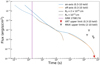 |
Fig. 9. Models of the HLE X-ray emission (0.3 − 10) keV of GW170817. Blue and orange lines denote on-axis and off-axis (θv = 15°) views and solid and dotted lines mark models with R0 = 2 × 1015 cm and R0 = 1013 cm, respectively. Swift-XRT (0.3–10) keV and MAXI (2–10) keV upper limits are shown by the gray and red triangles, respectively. The purple vertical line represents the trigger time of GRB 170817A with respect to the GW signal. A power-law structured jet is assumed (from Ghirlanda et al. 2019) with Γc = 251, θc = θE = 3.4°, EK,ISO = 2.5 × 1052 erg, and power-law slope kc = 3.5 and kE = 5.5 for the energy and bulk Lorentz factor, respectively. A SBPL with hνpeak = 100 keV, αs = 0.5, and βs = 1.3 is assumed. |
From Fig. 9 we can deduce that XRT would have been able to observe the HLE from the GRB 170817A: the earliest follow-up would grant a detection even for small emission radii (dashed lines in Fig. 9).
With the current follow-up timing, the emission, in the case of R0 = 2 × 1015 cm (solid lines in Fig. 9), appears to be marginally detectable. Uncertainty on the parameters of the jet structure are not included in this analysis. We conclude that the current X-ray follow-up observations of GW170817, starting at relatively late times with respect to the typical timescales of development of the HLE emission, cannot exclude the presence of the latter component while they constrain the emission radius to be ≲ 2 × 1015 cm.
A more stringent upper limit on the emission radius could be derived under the assumption that the observed γ-ray emission of GRB 170817A is produced by a standard GRB jet seen off-axis. In this case, the first photons of the HLE emission should be coincident with the time of arrival of the γ-ray photons. The start time of the HLE emission strongly depends on the emission radius (see Fig. 9). Within the uncertainties of our model we infer that a considerably small emission radius ≲5 × 1012 cm is required in order to produce an HLE emission starting at the trigger time of GRB 170817A. This result seems to support alternative interpretations, such as for example that the γ-ray emission of GRB 170817A was likely produced by the cocoon shock breakout (Kasliwal et al. 2017; Gottlieb et al. 2018; Nakar et al. 2018).
5. Summary and discussion
In this work we expand on the interpretation proposed in O20 of the steep decay and the plateau, often observed in γ-ray burst X-ray afterglows, as the HLE of the prompt emission produced by a structured jet. In this work we explore more realistic physical conditions: the finite duration of the emission (as compared to an infinitesimal duration considered in O20) and the possible contribution of a non-negligible latitude-dependent optical depth. The main development, with respect to O20, is that we consider the HLE as observed from any arbitrary viewing angle.
Our interpretation of the steep decay-plateau emission as HLE from a structured jet overcomes some of the difficulties of interpreting it as due to a long-lived millisecond magnetar whose ability to launch a jet is uncertain (Murguia-Berthier et al. 2014, 2017; Ciolfi et al. 2017, 2019; Ciolfi 2020; see however Mösta et al. 2020 who pointed out that accounting for neutrino transport in simulations may help the formation of a jet).
We show that while considering an emission of finite duration (Fig. 3) the main conclusions of O20 remain unchanged: a plateau following the steep decay phase appears when the observer is on-axis (or almost on-axis). It is worth noting that in our framework we considered an entire surface switching on at the same time, expanding while radiating, and then switching off at the same time. A more realistic situation could be that of a surface that switches on (and off) gradually in time from the axis to the wings, such that the core radiates earlier when R0 is small, and the wings radiate later when R0 is large. However, even in this case, a steep decay-plateau behavior would be expected, with a steep decay generated by the core at smaller radii and a plateau generated by the wings at larger radii.
The steep decay-plateau structure is preserved even when the effect of Thomson opacity in the emitting region is considered. However, in this case, in order to avoid a considerable suppression of the plateau emission (which being produced by the wings of the jet would suffer mostly from this effect), the emission should take place at large radii (e.g R0 ≳ 1015 cm). This condition agrees with the results of O20, namely that a large R0 is required in order to produce a plateau phase lasting more than ≈103 s, as is often observed8. Interestingly, a small emission radius would produce only a steep decay since the plateau would be absorbed.
In the context of emission of a finite duration, accounting for the opacity does not considerably impact the light curve, since the opacity at earlier times (i.e., smaller R0) affects only the emission at high latitudes, which do not contribute substantially to the total light curve (see Fig. 4). Therefore, in the present work we show that even when more realistic physical condition are considered, the results of O20 still hold. As pointed out in O20, with a reasonable choice of parameters, plateau duration up to a few 104 s can be recovered. Although this timescale can in principle account for the duration of the majority of the events, many of them could be characterized by longer lasting plateaus. One example is GRB060729, which is characterized by a plateau of ∼ 4 × 10⁴ s and a final power-law decaying tail observed up to 125 days after the γ-ray trigger (Grupe et al. 2007). While the duration of the plateau is compatible (albeit marginally) with the results in O20, the 125-day tail cannot be due to the HLE and likely results from the forward-shock emission which is expected to dominate at late times. It is important to stress here that the HLE model presented in O20 and in the present work does not suggest that the HLE is the only component determining the X-ray light curve, but rather that it may give a non-negligible (if not dominant) contribution during the plateau phase.
We note that in the context of the HLE model, an important aspect that has not been addressed in the present work is the expected spectral evolution of the source. Several studies reported a softening during the steep decay, which terminates at the onset of the plateau, where a hardening can eventually occur (Zhang et al. 2007; Liang et al. 2007). From a qualitative point of view, in our model, which involves a SBPL spectrum, the spectral evolution is governed by the evolution of the Doppler factor (see Fig. 2 in O20). Its decrease during the steep decay is expected to lead to a softening in the spectrum, as already pointed out in previous studies (Zhang et al. 2009; Genet & Granot 2009). Similarly, the constant (slightly increasing) trend of the Doppler factor during the plateau should lead to no evolution (or a slight hardening) of the spectrum. However, these considerations are based on the simplistic assumption of a spectrum that is uniform along the emitting surface and that does not evolve with time. A proper modeling of the spectral evolution along with the inclusion of the forward shock contribution will be explored in a future work. It is worth noting that recently, Panaitescu (2020), using a model similar in concept to that in O20 but with a more refined prescription for the spectrum, was successful in fitting the light curve of four GRBs (GRB061121, GRB060607A, GRB061110A and GRB061007) accounting also for their spectral evolution.
We also studied how the HLE emission light curve varies with the viewing angle and with the jet structure parameters (Sect. 4). We find the steep-plateau morphology to be characteristic of a small viewing angle (i.e., within the jet core aperture) while for off-core observers the light curve appears shallower than the (on-axis) steep decay and steeper than the (on-axis) plateau.
A possible consequence of our model is that GRBs with steep decay and plateau emission phases should be those preferentially observed within the jet core. GRBs observed off-core should present less prominent steep plateaus and should also appear (at the same distance) fainter. However, for instance, GRB130427A is one of the most energetic GRBs but without a clear steep decay-plateau light curve (von Kienlin 2013; Maselli et al. 2013, 2014). However, while a detailed study is beyond the scope of the present work, we notice that parameters like R0 and the opacity can in some configuration suppress the plateau component, or the HLE component can be outshone by a brighter forward shock emission.
For what concerns the onset of the off-axis emission, our results show that when fixing the structure, depending on the viewing angle, we expect the first photon to reach the observer with different delays with respect to the jet-launching time. In the context of GWs, this is important information both for the EM follow-up of GW events and for the search for GW signals triggered by GRBs (Dietz et al. 2013; Kelley et al. 2013; Salafia et al. 2017; Abbott et al. 2019; Burns et al. 2019; Hamburg et al. 2020). This is of particular interest when choosing the time window for searching for GWs in subthreshold analysis in connection with weak Fermi and Swift signals.
Furthermore, we consider that in those cases where the HLE emission is not quenched by compactness, its faint off-axis emission can, in principle, be observed by the present X-ray sky surveys such as eROSITA or the future proposed wide-field X-ray telescopes such as THESEUS. This is shown in particular in Fig. 8, where, assuming the model of GRB 100906A in O20, we can see that, up to z = 0.045 (LVC range for BNS merger), THESEUS and eROSITA are able to detect the HLE at large viewing angles. Therefore, for these instruments, the off-axis view of γ-ray burst prompt emission may result in the discovery of a new population of X-ray transients.
Finally, we focused on GW170817 and, with the aid of jet parameters derived by Ghirlanda et al. (2019), we modeled two possible X-ray HLE light curves for two limiting emission radii. We find that, provided R0 < 2 × 1015 cm, our model predictions are fully consistent with the MAXI and Swift-XRT observations, since the HLE is expected to be too faint for MAXI and would have already faded away before the XRT observation. Furthermore, considering the temporal onset of the off-axis emission measured from the GW arrival time, we conclude that in order to explain GRB 170817A as an off-axis prompt emission we would require a radius R0 < 5 × 1012 cm. This particularly small radius, along with the fact that the predicted on-axis maximum flux would have been very faint, suggests us that GRB 170817A is probably not the off-axis view of a standard γ-ray burst.
Namely larger than the temporal resolution of the detector.
A flattening in the decay of the HLE light curve in the case of a structured jet have been previously pointed out by Dyks et al. (2005).
Differently from O20, we choose here a smooth function for the power-law structure, which ensures the stability of our algorithm for the HLE computation.
The observer is assumed to lie in the x − z plane, without lack of generality thanks to the assumed axial symmetry.
Concerning the cosmological transformations, for the sake of simplicity and since they do not impact the final conclusions of this paper, we consider the source at z = 0.
For a better visualization, we show only some selected n = 13 out of N = 105 partial light curves, shifting in the figure their fluxes by a factor N/n to properly represent the contribution of the emission at different radii.
A source is expected to remain in the THESEUS-SXI field of view for about 100 − 1000 s, considering the instrument in survey mode.
A large radius is required also from spectral considerations when electron-synchrotron emission is considered (see e.g., Beniamini et al. 2018; Ghisellini et al. 2020).
Acknowledgments
We thank Stefan Johannes Grimm for the Einstein Telescope range, Giulia Stratta for the THESEUS-SXI limits and Samuele Ronchini for the discussion about some aspects of the modelling presented in this paper. The authors acknowledges the anonymous referee for her/his suggestions that help us to improve the presentation of our results. S. A. acknowledges the PRIN-INAF “Towards the SKA and CTA era: discovery, localization and physics of transient sources”. MB, SDO, GO acknowledge financial contribution from the agreement ASI-INAF n.2017-14-H.0. MB acknowledge financial support from MIUR (PRIN 2017 grant 20179ZF5KS). SA acknowledges the GRAvitational Wave Inaf TeAm – GRAWITA (P. I. E. Brocato). GO is thankful to INAF – Osservatorio Astronomico di Brera for kind hospitality during the completion of this work. This paper is supported by European Union’s Horizon 2020 research and innovation programme under grant agreement No 871158, project AHEAD2020.
References
- Abbott, B. P., Abbott, R., Abbott, T. D., et al. 2017a, ApJ, 848, L12 [Google Scholar]
- Abbott, B. P., Abbott, R., Abbott, T. D., et al. 2017b, ApJ, 848, L13 [NASA ADS] [CrossRef] [Google Scholar]
- Abbott, B. P., Abbott, R., Abbott, T. D., et al. 2018, Liv. Rev. Rel., 21, 3 [NASA ADS] [CrossRef] [Google Scholar]
- Abbott, B. P., Abbott, R., Abbott, T. D., et al. 2019, ApJ, 886, 75 [CrossRef] [Google Scholar]
- Abernathy, M., et al. 2011, Einstein Gravitational Wave Telescope Conceptual Design Study. ET-0106C-10, https://tds.ego-gw.it/ql/?c=7954 [Google Scholar]
- Abramowicz, M. A., Novikov, I. D., & Paczynski, B. 1991, ApJ, 369, 175 [NASA ADS] [CrossRef] [Google Scholar]
- Alexander, K. D., Margutti, R., Blanchard, P. K., et al. 2018, ApJ, 863, L18 [NASA ADS] [CrossRef] [Google Scholar]
- Aloy, M. A., Müller, E., Ibáñez, J. M., Martí, J. M., & MacFadyen, A. 2000, ApJ, 531, L119 [NASA ADS] [CrossRef] [PubMed] [Google Scholar]
- Aloy, M. A., Janka, H. T., & Müller, E. 2005, A&A, 436, 273 [NASA ADS] [CrossRef] [EDP Sciences] [Google Scholar]
- Amati, L., O’Brien, P., Götz, D., et al. 2018, Adv. Space Res., 62, 191 [Google Scholar]
- Beniamini, P., Barniol Duran, R., & Giannios, D. 2018, MNRAS, 476, 1785 [NASA ADS] [CrossRef] [Google Scholar]
- Beniamini, P., Duque, R., Daigne, F., & Mochkovitch, R. 2020a, MNRAS, 492, 2847 [CrossRef] [Google Scholar]
- Beniamini, P., Granot, J., & Gill, R. 2020b, MNRAS, 493, 3521 [CrossRef] [Google Scholar]
- Berger, E. 2014, ARA&A, 52, 43 [NASA ADS] [CrossRef] [Google Scholar]
- Bromberg, O., Nakar, E., Piran, T., & Sari, R. 2011, ApJ, 740, 100 [NASA ADS] [CrossRef] [Google Scholar]
- Burns, E., Goldstein, A., Hui, C. M., et al. 2019, ApJ, 871, 90 [CrossRef] [Google Scholar]
- Ciolfi, R. 2020, MNRAS, 495, L66 [CrossRef] [Google Scholar]
- Ciolfi, R., Kastaun, W., Giacomazzo, B., et al. 2017, Phys. Rev. D, 95, 063016 [NASA ADS] [CrossRef] [Google Scholar]
- Ciolfi, R., Kastaun, W., Kalinani, J. V., & Giacomazzo, B. 2019, Phys. Rev. D, 100, 023005 [CrossRef] [Google Scholar]
- Coulter, D. A., Foley, R. J., Kilpatrick, C. D., et al. 2017, Science, 358, 1556 [NASA ADS] [CrossRef] [Google Scholar]
- Dai, Z. G. 2004, ApJ, 606, 1000 [NASA ADS] [CrossRef] [Google Scholar]
- Dai, Z. G., & Lu, T. 1998a, A&A, 333, L87 [NASA ADS] [Google Scholar]
- Dai, Z. G., & Lu, T. 1998b, Phys. Rev. Lett., 81, 4301 [NASA ADS] [CrossRef] [Google Scholar]
- Dainotti, M. G., Cardone, V. F., & Capozziello, S. 2008, MNRAS, 391, L79 [NASA ADS] [CrossRef] [Google Scholar]
- Dall’Osso, S., Stratta, G., Guetta, D., et al. 2011, A&A, 526, A121 [NASA ADS] [CrossRef] [EDP Sciences] [Google Scholar]
- D’Avanzo, P., Salvaterra, R., Bernardini, M. G., et al. 2014, MNRAS, 442, 2342 [NASA ADS] [CrossRef] [Google Scholar]
- D’Avanzo, P., Campana, S., Salafia, O. S., et al. 2018, A&A, 613, L1 [NASA ADS] [CrossRef] [EDP Sciences] [Google Scholar]
- De Pasquale, M., Evans, P., Oates, S., et al. 2011, Adv. Space Res., 48, 1411 [CrossRef] [Google Scholar]
- Dietz, A., Fotopoulos, N., Singer, L., & Cutler, C. 2013, Phys. Rev. D, 87, 064033 [CrossRef] [Google Scholar]
- Dobie, D., Kaplan, D. L., Murphy, T., et al. 2018, ApJ, 858, L15 [NASA ADS] [CrossRef] [Google Scholar]
- Dyks, J., Zhang, B., & Fan, Y. Z. 2005, ArXiv e-prints [arXiv:astro-ph/0511699] [Google Scholar]
- Evans, P. A., Cenko, S. B., Kennea, J. A., et al. 2017, Science, 358, 1565 [NASA ADS] [CrossRef] [Google Scholar]
- Fan, Y., & Piran, T. 2006, MNRAS, 369, 197 [NASA ADS] [CrossRef] [Google Scholar]
- Fenimore, E. E., Madras, C. D., & Nayakshin, S. 1996, ApJ, 473, 998 [NASA ADS] [CrossRef] [Google Scholar]
- Genet, F., & Granot, J. 2009, MNRAS, 399, 1328 [NASA ADS] [CrossRef] [Google Scholar]
- Ghirlanda, G., Salafia, O. S., Paragi, Z., et al. 2019, Science, 363, 968 [NASA ADS] [CrossRef] [Google Scholar]
- Ghisellini, G. 2013, Radiative Processes in High Energy Astrophysics, 873 (Switzerland: Springer International Publishing) [Google Scholar]
- Ghisellini, G., Ghirlanda, G., Nava, L., & Firmani, C. 2007, ApJ, 658, L75 [NASA ADS] [CrossRef] [Google Scholar]
- Ghisellini, G., Ghirlanda, G., Oganesyan, G., et al. 2020, A&A, 636, A82 [CrossRef] [EDP Sciences] [Google Scholar]
- Goldstein, A., Veres, P., Burns, E., et al. 2017, ApJ, 848, L14 [NASA ADS] [CrossRef] [Google Scholar]
- Gottlieb, O., Nakar, E., Piran, T., & Hotokezaka, K. 2018, MNRAS, 479, 588 [NASA ADS] [Google Scholar]
- Grupe, D., Gronwall, C., Wang, X.-Y., et al. 2007, ApJ, 662, 443 [NASA ADS] [CrossRef] [Google Scholar]
- Hajela, A., Margutti, R., Alexander, K. D., et al. 2019, ApJ, 886, L17 [NASA ADS] [CrossRef] [Google Scholar]
- Hamburg, R., Fletcher, C., Burns, E., et al. 2020, ApJ, 893, 100 [CrossRef] [Google Scholar]
- Hernanz, M., Brandt, S., Feroci, M., et al. 2018, SPIE Conf. Ser., 10699, 1069948 [Google Scholar]
- Hörmander, L. 2015, The Analysis of Linear Partial Differential Operators I: Distribution Theory and Fourier Analysis, Classics in Mathematics (Berlin Heidelberg: Springer) [Google Scholar]
- Ioka, K., & Nakamura, T. 2019, MNRAS, 487, 4884 [NASA ADS] [CrossRef] [Google Scholar]
- Izzo, L., Muccino, M., Zaninoni, E., Amati, L., & Della Valle, M. 2015, A&A, 582, A115 [NASA ADS] [CrossRef] [EDP Sciences] [Google Scholar]
- Jia, L.-W., Uhm, Z. L., & Zhang, B. 2016, ApJS, 225, 17 [CrossRef] [Google Scholar]
- Kasliwal, M. M., Nakar, E., Singer, L. P., et al. 2017, Science, 358, 1559 [NASA ADS] [CrossRef] [Google Scholar]
- Kelley, L. Z., Mandel, I., & Ramirez-Ruiz, E. 2013, Phys. Rev. D, 87, 123004 [NASA ADS] [CrossRef] [Google Scholar]
- Khabibullin, I., Sazonov, S., & Sunyaev, R. 2012, MNRAS, 426, 1819 [NASA ADS] [CrossRef] [Google Scholar]
- Kumar, P., & Panaitescu, A. 2000, ApJ, 541, L51 [NASA ADS] [CrossRef] [Google Scholar]
- Kumar, P., & Piran, T. 2000, ApJ, 535, 152 [NASA ADS] [CrossRef] [Google Scholar]
- Kumar, P., & Zhang, B. 2015, Phys. Rep., 561, 1 [Google Scholar]
- Lamb, G. P., Lyman, J. D., Levan, A. J., et al. 2019, ApJ, 870, L15 [NASA ADS] [CrossRef] [Google Scholar]
- Lazzati, D., & Begelman, M. C. 2005, ApJ, 629, 903 [NASA ADS] [CrossRef] [Google Scholar]
- Lazzati, D., & Perna, R. 2019, ApJ, 881, 89 [NASA ADS] [CrossRef] [Google Scholar]
- Lazzati, D., Deich, A., Morsony, B. J., & Workman, J. C. 2017a, MNRAS, 471, 1652 [NASA ADS] [CrossRef] [Google Scholar]
- Lazzati, D., López-Cámara, D., Cantiello, M., et al. 2017b, ApJ, 848, L6 [NASA ADS] [CrossRef] [Google Scholar]
- Lazzati, D., Perna, R., Morsony, B. J., et al. 2018, Phys. Rev. Lett., 120, 241103 [NASA ADS] [CrossRef] [PubMed] [Google Scholar]
- Li, L., Wu, X.-F., Huang, Y.-F., et al. 2015, ApJ, 805, 13 [CrossRef] [Google Scholar]
- Liang, E.-W., Zhang, B.-B., & Zhang, B. 2007, ApJ, 670, 565 [NASA ADS] [CrossRef] [Google Scholar]
- Liang, E.-W., Racusin, J. L., Zhang, B., Zhang, B.-B., & Burrows, D. N. 2008, ApJ, 675, 528 [NASA ADS] [CrossRef] [Google Scholar]
- Lithwick, Y., & Sari, R. 2001, ApJ, 555, 540 [NASA ADS] [CrossRef] [Google Scholar]
- Lyman, J. D., Lamb, G. P., Levan, A. J., et al. 2018, Nat. Astron., 2, 751 [NASA ADS] [CrossRef] [Google Scholar]
- Maggiore, M., Van Den Broeck, C., Bartolo, N., et al. 2020, JCAP, 2020, 050 [CrossRef] [Google Scholar]
- Margutti, R., Zaninoni, E., Bernardini, M. G., et al. 2013, MNRAS, 428, 729 [NASA ADS] [CrossRef] [Google Scholar]
- Margutti, R., Alexander, K. D., Xie, X., et al. 2018, ApJ, 856, L18 [NASA ADS] [CrossRef] [Google Scholar]
- Maselli, A., Beardmore, A. P., Lien, A. Y., et al. 2013, GRB Coordinates Netw., 14448, 1 [Google Scholar]
- Maselli, A., Melandri, A., Nava, L., et al. 2014, Science, 343, 48 [NASA ADS] [CrossRef] [Google Scholar]
- Matsumoto, T., Nakar, E., & Piran, T. 2019, MNRAS, 486, 1563 [CrossRef] [Google Scholar]
- Matzner, C. D. 2003, MNRAS, 345, 575 [NASA ADS] [CrossRef] [Google Scholar]
- Melandri, A., Covino, S., Rogantini, D., et al. 2014, A&A, 565, A72 [NASA ADS] [CrossRef] [EDP Sciences] [Google Scholar]
- Merloni, A., Predehl, P., Becker, W., et al. 2012, ArXiv e-prints [arXiv:1209.3114] [Google Scholar]
- Metzger, B. D., & Piro, A. L. 2014, MNRAS, 439, 3916 [NASA ADS] [CrossRef] [Google Scholar]
- Metzger, B. D., Giannios, D., Thompson, T. A., Bucciantini, N., & Quataert, E. 2011, MNRAS, 413, 2031 [NASA ADS] [CrossRef] [Google Scholar]
- Mooley, K. P., Deller, A. T., Gottlieb, O., et al. 2018a, Nature, 561, 355 [NASA ADS] [CrossRef] [PubMed] [Google Scholar]
- Mooley, K. P., Nakar, E., Hotokezaka, K., et al. 2018b, Nature, 554, 207 [NASA ADS] [CrossRef] [PubMed] [Google Scholar]
- Morsony, B. J., Lazzati, D., & Begelman, M. C. 2007, ApJ, 665, 569 [NASA ADS] [CrossRef] [Google Scholar]
- Mösta, P., Radice, D., Haas, R., Schnetter, E., & Bernuzzi, S. 2020, ArXiv e-prints [arXiv:2003.06043] [Google Scholar]
- Murguia-Berthier, A., Montes, G., Ramirez-Ruiz, E., De Colle, F., & Lee, W. H. 2014, ApJ, 788, L8 [CrossRef] [Google Scholar]
- Murguia-Berthier, A., Ramirez-Ruiz, E., Montes, G., et al. 2017, ApJ, 835, L34 [NASA ADS] [CrossRef] [Google Scholar]
- Nakar, E. 2019, ArXiv e-prints [arXiv:1912.05659] [Google Scholar]
- Nakar, E., Gottlieb, O., Piran, T., Kasliwal, M. M., & Hallinan, G. 2018, ApJ, 867, 18 [NASA ADS] [CrossRef] [Google Scholar]
- Nousek, J. A., Kouveliotou, C., Grupe, D., et al. 2006, ApJ, 642, 389 [NASA ADS] [CrossRef] [Google Scholar]
- Oates, S. R., Page, M. J., Schady, P., et al. 2011, MNRAS, 412, 561 [NASA ADS] [CrossRef] [Google Scholar]
- O’Brien, P. T., Willingale, R., Osborne, J., et al. 2006, ApJ, 647, 1213 [NASA ADS] [CrossRef] [Google Scholar]
- Oganesyan, G., Ascenzi, S., Branchesi, M., et al. 2020, ApJ, 893, 88 [CrossRef] [Google Scholar]
- Panaitescu, A. 2008, MNRAS, 383, 1143 [NASA ADS] [CrossRef] [Google Scholar]
- Panaitescu, A. 2020, ApJ, 895, 39 [CrossRef] [Google Scholar]
- Panaitescu, A., & Vestrand, W. T. 2011, MNRAS, 414, 3537 [NASA ADS] [CrossRef] [Google Scholar]
- Piran, T. 1999, Phys. Rep., 314, 575 [NASA ADS] [CrossRef] [Google Scholar]
- Piran, T. 2004, Rev. Mod. Phys., 76, 1143 [NASA ADS] [CrossRef] [Google Scholar]
- Ramirez-Ruiz, E., Celotti, A., & Rees, M. J. 2002, MNRAS, 337, 1349 [NASA ADS] [CrossRef] [Google Scholar]
- Reitze, D., Adhikari, R. X., Ballmer, S., et al. 2019, BAAS, 51, 35 [NASA ADS] [Google Scholar]
- Resmi, L., Schulze, S., Ishwara-Chandra, C. H., et al. 2018, ApJ, 867, 57 [NASA ADS] [CrossRef] [Google Scholar]
- Rossi, E., Lazzati, D., & Rees, M. J. 2002, MNRAS, 332, 945 [NASA ADS] [CrossRef] [Google Scholar]
- Ruderman, M. 1975, in Seventh Texas Symposium on Relativistic Astrophysics, eds. P. G. Bergman, E. J. Fenyves, & L. Motz, 262, 164 [Google Scholar]
- Salafia, O. S., Ghisellini, G., Pescalli, A., Ghirland, G., & Nappo, F. 2015, MNRAS, 450, 3549 [NASA ADS] [CrossRef] [Google Scholar]
- Salafia, O. S., Colpi, M., Branchesi, M., et al. 2017, ApJ, 846, 62 [NASA ADS] [CrossRef] [Google Scholar]
- Salafia, O. S., Ghirlanda, G., Ascenzi, S., & Ghisellini, G. 2019, A&A, 628, A18 [NASA ADS] [CrossRef] [EDP Sciences] [Google Scholar]
- Salafia, O. S., Barbieri, C., Ascenzi, S., & Toffano, M. 2020, A&A, 636, A105 [CrossRef] [EDP Sciences] [Google Scholar]
- Sarin, N., Lasky, P. D., & Ashton, G. 2020, Phys. Rev. D, 101, 063021 [CrossRef] [Google Scholar]
- Savchenko, V., Ferrigno, C., Kuulkers, E., et al. 2017, ApJ, 848, L15 [NASA ADS] [CrossRef] [Google Scholar]
- Schmidt, W. K. H. 1978, Nature, 271, 525 [CrossRef] [Google Scholar]
- Siegel, D. M., & Ciolfi, R. 2016a, ApJ, 819, 14 [NASA ADS] [CrossRef] [Google Scholar]
- Siegel, D. M., & Ciolfi, R. 2016b, ApJ, 819, 15 [NASA ADS] [CrossRef] [Google Scholar]
- Sugita, S., Kawai, N., Serino, M., et al. 2017, GRB Coordinates Netw., 21555, 1 [Google Scholar]
- Tagliaferri, G., Goad, M., Chincarini, G., et al. 2005, Nature, 436, 985 [NASA ADS] [CrossRef] [PubMed] [Google Scholar]
- Tang, C.-H., Huang, Y.-F., Geng, J.-J., & Zhang, Z.-B. 2019, ApJS, 245, 1 [NASA ADS] [CrossRef] [Google Scholar]
- Troja, E., Piro, L., van Eerten, H., et al. 2017, Nature, 551, 71 [NASA ADS] [CrossRef] [Google Scholar]
- Troja, E., Piro, L., Ryan, G., et al. 2018, MNRAS, 478, L18 [NASA ADS] [CrossRef] [Google Scholar]
- von Kienlin, A. 2013, GRB Coordinates Netw., 14473, 1 [Google Scholar]
- Wei, J., Cordier, B., Antier, S., et al. 2016, ArXiv e-prints [arXiv:1610.06892] [Google Scholar]
- Willingale, R., O’Brien, P. T., Osborne, J. P., et al. 2007, ApJ, 662, 1093 [NASA ADS] [CrossRef] [Google Scholar]
- Xie, X., & MacFadyen, A. 2019, ApJ, 880, 135 [NASA ADS] [CrossRef] [Google Scholar]
- Yu, Y.-W., Cheng, K. S., & Cao, X.-F. 2010, ApJ, 715, 477 [NASA ADS] [CrossRef] [Google Scholar]
- Yu, Y.-W., Zhang, B., & Gao, H. 2013, ApJ, 776, L40 [NASA ADS] [CrossRef] [Google Scholar]
- Yuan, W., Zhang, C., Feng, H., et al. 2015, ArXiv e-prints [arXiv:1506.07735] [Google Scholar]
- Zaninoni, E., Bernardini, M. G., Margutti, R., Oates, S., & Chincarini, G. 2013, A&A, 557, A12 [NASA ADS] [CrossRef] [EDP Sciences] [Google Scholar]
- Zhang, B., & Mészáros, P. 2001, ApJ, 552, L35 [NASA ADS] [CrossRef] [Google Scholar]
- Zhang, B., & Mészáros, P. 2002, ApJ, 571, 876 [NASA ADS] [CrossRef] [Google Scholar]
- Zhang, W., Woosley, S. E., & MacFadyen, A. I. 2003, ApJ, 586, 356 [NASA ADS] [CrossRef] [Google Scholar]
- Zhang, B., Fan, Y. Z., Dyks, J., et al. 2006, ApJ, 642, 354 [NASA ADS] [CrossRef] [Google Scholar]
- Zhang, B.-B., Liang, E.-W., & Zhang, B. 2007, ApJ, 666, 1002 [NASA ADS] [CrossRef] [Google Scholar]
- Zhang, B.-B., Zhang, B., Liang, E.-W., & Wang, X.-Y. 2009, ApJ, 690, L10 [CrossRef] [Google Scholar]
Appendix A: EATRs equation
A central aspect of our analysis concerns the identification of the EATRs. In this Appendix we describe the algorithm that we employed to calculate them.
We consider a general axisymmetric surface described by the function R = R(θ). This surface corresponds to the emitting surface in our problem. We identify a cartesian coordinate system 𝒦 whose z-axis coincides with the surface’s symmetry axis. In this system, the emitting surface can be described by the following parametrization:
 (A.1)
(A.1)
We choose the orientation of the x and y axis of this frame such that the observer lies on the x − z plane (due to the axial symmetry this choice do not imply any loss of generality).
Now we define a second reference frame 𝒦′ obtained applying on 𝒦 a rotation around the y axis of an angle θv, such that z′ coincides with the observer line of sight. The coordinates of a surface point in the new frames are:
 (A.2)
(A.2)
In particular we are interested in those surface points that have the same z′, because they are those that have the same distance from the observer and consequently those emitting photons with the same arrival time. We consider the travel time of a photon emitted from the central engine at jet launching time as a reference time, which corresponds to t0 = dL/c. The travel time of a photon emitted from a point with a given z′ is thus tobs = tem − (dL − z′)/c − t0, where tem is the time (measured from t0) at which the emission occurs. Solving for z′ we obtain:
 (A.3)
(A.3)
This equation is the EATR equation, and its solution, which is obtained numerically, represents a curve θ = θ(ϕ) on the emitting surface that corresponds to the EATR at that time.
Appendix B: Derivation of the flux
B.1. Infinitesimal duration pulse
In this Appendix we report the proof of Eq. (5). As in Kumar & Zhang (2015) we start from the general expression of the flux in terms of integral of specific intensity over the observer solid angle:
 (B.1)
(B.1)
It is worth noting that the factor cos θobs, which represents the projection of the emitting surface elementary area along the observer line of sight, is correct only for a spherical surface, and so we substitute it with the more general expression  . Moreover, this factor must be present only if the emitting region is optically thick. This is due to the fact that when the matter is optically thin, radiation can always reach the observer even if the normal
  to the emitting surface is orthogonal to the line of sight, because all the photons can freely stream out of the edge of the surface (even if we approximate the emitting surface as a surface, the elementary emitters are always contained within a volume; e.g., see Ghisellini 2013). On the other hand, when the matter is optically thick, only a negligible amount of radiation (proportional to the negligible width of the emitting region) will stream out from the surface’s edge, and most of the contribution will come from the fraction of the surface "exposed" to the observer. In order to take into account this effect we define the optical depth-dependent projection factor:
 (B.2)
(B.2)
where the first term represents the fraction of the emitting surface "exposed" to the observer and the second term represents the fraction not exposed to the observer, whose contribution is quenched by the factor exp−τ, where τ is the optical depth. When the opacity is neglected (as in Sect. 2) the projection factor is simply P(θ, ϕ, τ = 0) = 1, while in the optically thick limit (i.e. τ ≫ 1)  . Note that 0 ≤ P(θ, ϕ, τ)≤1.
The other substitutions we apply involve the solid angle, which is written in terms of elementary area and source distance, 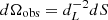 , and the specific intensity, which is written in terms of specific intensity in the comoving frame. Thus we obtain:
 (B.3)
(B.3)
Now we consider the limiting case in which all the radiation is emitted in an impulse centered at the time tem with infinitesimal duration in the CoE frame. We can write the intensity in terms of a Dirac delta of time:
 (B.4)
(B.4)
where  is the total energy radiated in the comoving frame at frequency ν′ = ν(1 + z)/D(θ, ϕ) by the elementary area at θ, t is the time variable in the CoE frame, while tem is a constant corresponding to the actual emission time in which the emission takes place.
  can be further decoupled in two different factors: a frequency-independent part and a spectral part:
 (B.5)
(B.5)
where ϵ(θ) is the same term appearing in Eq. (2) (Eq. (1)) describing the structure in energy of the emitting surface,  represents the spectrum normalized to 1 at
  , and
, and  is a constant corresponding to
  at
at  and θ = 0. It is worth noting that although the comoving frame spectrum
  is taken as uniform across the emitting surface (hence, it does not depend on θ and ϕ), when we integrate along the EATR we have to take into account that radiation from different parts of the surface is blueshifted by different factors. Therefore, the integrands in Eq. (B.3) have to be evaluated in ν′ = ν(1 + z)/D(θ, ϕ), fixing the observer frame frequency ν. This introduces in the
  a further θ and ϕ dependence (through ν′), which preserves the shape of the spectrum and shifts it by a D(θ, ϕ) factor along the ν-axis.
At this point, we can write t = DΓtobs (see Eq. (11) in Kumar & Zhang 2015) to make the dependence of the observation time tobs explicit, such that Eq. (B.4) writes as
![Mathematical equation: $$ \begin{aligned}&I^{\prime }_{\nu ^{\prime }}(\nu ^{\prime }, \theta , t_{\rm obs}) = \eta ^{\prime }_{\nu ^{\prime }}(\nu ^{\prime }, \theta )\delta [D(\theta , \phi )\Gamma (\theta )t_{\rm obs}-t_{\rm em}]\nonumber \\&\qquad \qquad \quad = \eta ^{\prime }_{\nu ^{\prime }}(\nu ^{\prime })\delta [h(\theta , \phi )]. \end{aligned} $$](/articles/aa/full_html/2020/09/aa38265-20/aa38265-20-eq44.gif) (B.6)
(B.6)
It is worth noting that the solution of the equation h(θ, ϕ) = 0 identifies a curve θ = θ(ϕ) on the emitting surface, which represents the EATR at a given tobs.
Now, taking into account the last substitution, we can write the flux density as
![Mathematical equation: $$ \begin{aligned} F_\nu (t_{\rm obs}) = \frac{1}{\mathrm{d}^2_L(1+z)^3}\int _S \mathrm{d}S P(\theta , \phi , \tau ) \eta ^{\prime }_{\nu ^{\prime }}(\nu ^{\prime })D^{3}(\theta , \phi )\delta [h(\theta , \phi )]. \end{aligned} $$](/articles/aa/full_html/2020/09/aa38265-20/aa38265-20-eq45.gif) (B.7)
(B.7)
Now the Dirac delta allows us to transform the surface integral into a line integral on the EATR. Due to the property of the delta of a multivariate function (Hörmander 2015) we finally obtain
 (B.8)
(B.8)
Given this equation, an interesting case worth studying is that of a power-law spectrum, that we can describe as:
![Mathematical equation: $$ \begin{aligned} \eta ^{\prime }_{\nu ^{\prime }}[\nu (1+z)/D, \theta ] = \eta ^{\prime }_{\nu ^{\prime }_0}\epsilon (\theta )\left(\frac{\nu ^{\prime }_0}{\nu }\right)^{\beta _s}\frac{D^{\beta _s}(\theta , \phi )}{(1+z)^{\beta _s}}, \end{aligned} $$](/articles/aa/full_html/2020/09/aa38265-20/aa38265-20-eq47.gif) (B.9)
(B.9)
where βs is the power-law spectral index. With this spectrum the equation for the flux writes as:
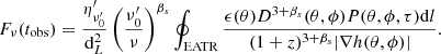 (B.10)
We can test this equation on the limiting case of a spherical ejecta. In this case we set θv = 0, ϵ(θ) = 1 and we have also that ∂θ(…) = 0. In this case, the EATRs correspond to circles with length L = 2πR sin θ, while the projection factor at a given point of the surface is P(θ, ϕ, τ = 0) = 1 (or  in the optically thick regime) and the gradient is |∇h(θ, ϕ)| = DΓ sin θ/c. Considering the previous substitution we obtain:
![Mathematical equation: $$ \begin{aligned} F_\nu (t_{\rm obs}) = \frac{2\pi \eta ^{\prime }_{\nu ^{\prime }_0}Rc}{\mathrm{d}^2_L[\Gamma (1+z)]^{3+\beta _s}}\left(\frac{\nu ^{\prime }_o}{\nu }\right)^{\beta _s}t^{2+\beta _s}_{\rm em}t^{-(2+\beta _s)}_{\rm obs} , \end{aligned} $$](/articles/aa/full_html/2020/09/aa38265-20/aa38265-20-eq50.gif) (B.11)
(B.11)
which is consistent with the classical result of Kumar & Panaitescu (2000).
We consider also the flux described by the SBPL function in Eq. (8). In this case we have:
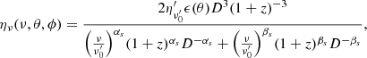 (B.12)
where αs and βs are the spectral indices below and above the peak. Here we hide the θ and ϕ dependence of the Doppler factor for the sake of compactness. With this spectrum profile the flux writes as:
![Mathematical equation: $$ \begin{aligned}&F_\nu (t_{\rm obs}) = \frac{2\eta ^{\prime }_{\nu ^{\prime }_0}}{\mathrm{d}^2_L(1+z)^3}\nonumber \\&\qquad \qquad \times \oint _{EATR} \frac{\epsilon (\theta )D^{3}(\theta , \phi )P(\theta , \phi , \tau )\mathrm{d}l}{\Bigl [\Bigl (\frac{\nu (1+z)}{\nu ^{\prime }_0D}\Bigr )^{\alpha _s} +\Bigl (\frac{\nu (1+z)}{\nu ^{\prime }_0D}\Bigr )^{\beta _s}\Bigr ]|\nabla {h}(\theta , \phi )|}. \end{aligned} $$](/articles/aa/full_html/2020/09/aa38265-20/aa38265-20-eq52.gif) (B.13)
(B.13)
B.2. Finite duration pulse
To account for a finite duration pulse we adopt the following approximate approach:
-
we define a specific intensity temporal profile
 . The total emitted energy per unit area, per unit frequency, and per unit solid angle writes as:
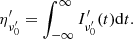 (B.14)
 -
We divide the flux profile in N time intervals of finite length Δtem and central values tem, i with i = 1, …, N. The energy per unit area radiated in the ith time interval is:
 (B.15)
By definition we have that:
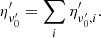 (B.16)
 -
We introduce a function
 which approximates the flux profile and is defined as a Dirac comb:
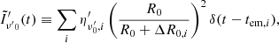 (B.17)
where ΔR0, i ≡ R0, i − R0 is the difference between the radius of the first and the ith emitting surface at θ = 0. The terms in parenthesis have been added since in the case of an internal dissipation mechanism, such as that considered here, the emitters are expected to conserve in number and dilute in time while the emitting surface expands. With the prescription in Eq. (B.17), the specific intensity approximates as
 .
. -
We express the final flux as the superimposition of the N impulses of the Dirac comb:
![Mathematical equation: $$ \begin{aligned}&F_\nu = \frac{1}{\mathrm{d}^2_L(1+z)^3}\int _S\mathrm{d}S P(\theta , \phi , \tau ) D^{3}(\theta , \phi ){\tilde{I}^{\prime }}_{{\nu ^{\prime }}_0}(t)\epsilon (\theta )\nonumber \\&\qquad \times S^{\prime }_{\nu ^{\prime }}[\nu (1+z)/D(\theta , \phi )]. \end{aligned} $$](/articles/aa/full_html/2020/09/aa38265-20/aa38265-20-eq60.gif) (B.18)
(B.18)Here S = S1 ∪ … ∪ SN, where Si is the emitting surface of the ith delta of the comb.
It is worth noting that in this approach Eq. (B.16) guarantees that the total energy of the pulse is preserved regardless of the value of N.
Appendix C: Optical depth derivation
In this section we derive Eq. (9). We consider a shell of material of inner radius R(θ) and width ΔR(θ) and a photon emitted at R. We limit ourselves to photons traveling radially outwards, as the emission is always dominated by them. The optical depth of the shell due to Thomson scattering will be
 (C.1)
(C.1)
where ne(r, θ) is the electron number density and dR(θ) is the length traveled by a photon within the shell. As the shell is moving at the velocity βc in the same time in which the photon travels a distance dr = cdt, the shell travels a distance drs(θ) = β(θ)cdt, such that dR(θ) = dr − drs = (1 − β)cdt (Abramowicz et al. 1991).
In the meantime, the jet expansion causes matter to dilute, with the electron density decreasing as ne(r, θ) = ne(R, θ)(r/R)−2.
The value of ne(R, θ) can be obtained considering that in a time interval Δt the amount of isotropic equivalent mass of charged particles passing through r0 is:
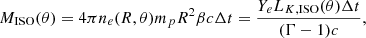 (C.2)
(C.2)
where Ye is the electron fraction and LK, ISO is the isotropic equivalent kinetic luminosity defined as LK, ISO(θ) = (Γ(θ)−1)M(θ)c2/Δt. Solving for ne(R, θ) we obtain:
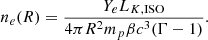 (C.3)
(C.3)
Substituting the density profile in Eq. (C.1) we obtain:
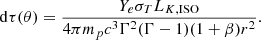 (C.4)
(C.4)
The optical depth is then obtained integrating Eq. (C.4):
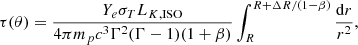 (C.5)
(C.5)
where ΔR/(1 − β) = ΔR(1 + β)Γ2 is the length traveled by the photon to escape the shell. Solving the integral we obtain:
![Mathematical equation: $$ \begin{aligned} \tau (\theta ) = \frac{Y_e \sigma _T L_{K, \mathrm{ISO}}}{4\pi m_p c^3\Gamma ^2(\Gamma -1)(1+\beta )}\Bigl [\frac{1}{R} - \frac{1}{R + \Delta R(1+\beta )\Gamma ^2}\Bigr ], \end{aligned} $$](/articles/aa/full_html/2020/09/aa38265-20/aa38265-20-eq66.gif) (C.6)
(C.6)
where the width of the shell is determined by the duration of the central engine as ΔR(θ) = β(θ)cΔTengine.
Appendix D: Power-law structures
In this Appendix we provide light curves for two different power-law structures. Finally, Figs. D.1 and D.2 show the light curves obtained by a power-law structure with k = 2 and k = 5, respectively. In both cases the qualitative behavior is the same as in the fiducial model. However, the k = 2 light curve presents more similarities between different viewing angles and a less varying slope in time. As expected, the sharp structure k = 5 is closer to the Gaussian model.
All Figures
|
Fig. 1. Pictorial representation of the system under study. The emitting surface is shown in red, the reference frame 𝒦 is in black, and the frame 𝒦′, with its z′ axis aligned with the line of sight, is represented in blue. The green circle shows an example of EATR. |
| In the text | |
|
Fig. 2. Equal arrival time rings (top panels) and corresponding light curves (bottom panels) for three configurations of the viewing angle (from left to right), θv = 0° (on-axis), θv = θc (edge-of-the-core), and θv = 3 × θc (off-axis). Top panels: polar plot of the emitting surface. The black circle shows the physical limit of the core of the jet. The black cross shows the observer line of sight. The colored curves are the EATRs at ten arbitrary sampling times. Bottom panels: light curve normalized at its maximum value (corresponding to the on-axis observer at the first sampled epoch). The colored dots represent the flux emitted by the corresponding colored EATRs in the top panel. The structured jet assumed for this test case has a Gaussian structure with Γc = 100, θc = θE = 3°, R0 = 1015 cm. The comoving emission spectrum is described by a SBPL spectrum with αs = 0.2 and βs = 1.3. |
| In the text | |
|
Fig. 3. Light curve for finite-duration emission. The case refers to an on-axis observer. The dashed colored light curves corresponding to n = 13 selected infinitesimal pulses out of the total N = 105 composing the finite-duration emission episode. Partial fluxes have been multiplied by a factor N/n in order to better visualize the contribution to the final emission at different radii. Colors identify the ΔR0, i (Δt) with respect to the initial R0 (tem) at which the first pulse is emitted. The black solid line is the final light curve made by the sum of the partial ones. We assume a Gaussian jet with parameters Γc = 100, θc = θE = 3°, R0 = 1013 cm and the pulse duration in the CoE frame ΔT = 105 s. A SBPL spectrum with αs = 0.2 and βs = 1.3 is assumed. |
| In the text | |
|
Fig. 4. Same as Fig. 3 but with the effect of a non-negligible and latitude-dependent opacity. The parameters for the optical depth are: Ye = 1, EK,ISO = 1054 erg and ΔTengine = 30 s. |
| In the text | |
|
Fig. 5. Light curves obtained varying Γc and θc at fixed R0 = 1015 cm, at different viewing angles. Light curves corresponding to viewing angles θv = 0, θc, 3θc are shown in blue, orange, and green, respectively. Continuous curves denote the fiducial model, with Γc = 100, θc = 3°. The structure is Gaussian and the spectrum is a SBPL function with αs = 0.2 and βs = 1.3. The light curves are those at ν = 10 keV normalized to the maximum value of the on-axis case and the time is relative to the time of arrival of the first photon. For better visualization, we translated the time such that the first photons arrive at 10−1 s. |
| In the text | |
|
Fig. 6. Same as Fig. 5 but with R0 = 1014 cm. In the off-axis case (θv = 3θc) the emission is quenched as described in the text (note the different y-axis scale with respect to Fig. 5). |
| In the text | |
|
Fig. 7. On-axis (θv = 0 × θc), edge (θv = θc), and off-axis (θv = 3 × θc) views of HLE (continuous line) and forward shock (dashed lines) models used in O20 to fit the light curve of GRB 100906A. The light curves are integrated in the energy range 0.5 − 10 keV. HLE model parameters: Γc = 160, R0 = 3 × 1015 cm and θc = 3.3° and θE = 4.4°, spectrum: SBPL, αs = 0.67, βs = 3.0 and νpeak = 100 keV, jet structure: Gaussian. Forward shock model parameters: n = 15 cm−3, p = 2.1, ϵe = 0.03, ϵB = 2 × 10⁻², EK,ISO = 5 × 1053 erg. |
| In the text | |
|
Fig. 8. Peak flux vs. viewing angle of the HLE of GRB 100906A assuming the same structure derived in O20. Circles, diamonds, and crosses represent the same model at three different redshifts: z = 1.730 (actual redshift of GRB 100906A), z = 0.045 (Advanced LIGO and Virgo range for BNS mergers), and z = 0.5 (ET range for BNS mergers), respectively. The color code denotes the logarithm of the time of the peak in the observer frame. Red continuous and red dashed lines mark the flux limit of THESEUS-SXI integrated in 103 s and 102 s, respectively. Black dashed line marks the flux limit of eROSITA integrated in 40 s. Verical dotted line marks θc. |
| In the text | |
|
Fig. 9. Models of the HLE X-ray emission (0.3 − 10) keV of GW170817. Blue and orange lines denote on-axis and off-axis (θv = 15°) views and solid and dotted lines mark models with R0 = 2 × 1015 cm and R0 = 1013 cm, respectively. Swift-XRT (0.3–10) keV and MAXI (2–10) keV upper limits are shown by the gray and red triangles, respectively. The purple vertical line represents the trigger time of GRB 170817A with respect to the GW signal. A power-law structured jet is assumed (from Ghirlanda et al. 2019) with Γc = 251, θc = θE = 3.4°, EK,ISO = 2.5 × 1052 erg, and power-law slope kc = 3.5 and kE = 5.5 for the energy and bulk Lorentz factor, respectively. A SBPL with hνpeak = 100 keV, αs = 0.5, and βs = 1.3 is assumed. |
| In the text | |
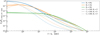 |
Fig. D.1. Same as Fig. 5 but with a power-law structure with k = 2. |
| In the text | |
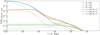 |
Fig. D.2. Same as Fig. 5 but with a power-law structure with k = 5. |
| In the text | |
Current usage metrics show cumulative count of Article Views (full-text article views including HTML views, PDF and ePub downloads, according to the available data) and Abstracts Views on Vision4Press platform.
Data correspond to usage on the plateform after 2015. The current usage metrics is available 48-96 hours after online publication and is updated daily on week days.
Initial download of the metrics may take a while.