| Issue |
A&A
Volume 640, August 2020
|
|
|---|---|---|
| Article Number | A43 | |
| Number of page(s) | 10 | |
| Section | Astrophysical processes | |
| DOI | https://doi.org/10.1051/0004-6361/202038166 | |
| Published online | 10 August 2020 | |
Inferring the origins of the pulsed γ-ray emission from the Crab pulsar with ten-year Fermi-LAT data⋆
Institute for Experimental Physics, Department of Physics, University of Hamburg, Luruper Chaussee 149, 22761 Hamburg, Germany
e-mail: This email address is being protected from spambots. You need JavaScript enabled to view it.
Received:
14
April
2020
Accepted:
6
June
2020
Abstract
Context. The Crab pulsar is a bright γ-ray source, which has been detected at photon energies up to ∼1 TeV. Its phase-averaged and phase-resolved γ-ray spectra below 10 GeV exhibit exponential cutoffs, while those above 10 GeV apparently follow simple power laws.
Aims. We re-visit the γ-ray properties of the Crab pulsar with ten-year Fermi Large Area Telescope (LAT) data in the range of 60 MeV–500 GeV. With the phase-resolved spectra, we investigate the origins and mechanisms responsible for the emissions.
Methods. The phaseograms were reconstructed for different energy bands and further analysed using a wavelet decomposition. The phase-resolved energy spectra were combined with the observations of ground-based instruments, such as MAGIC and VERITAS, to achieve a larger energy converage. We fitted power-law models to the overlapping energy spectra from 10 GeV to ∼1 TeV. In the fit, we included a relative cross-calibration of energy scales between air-shower-based gamma-ray telescopes with the orbital pair-production telescope from the Fermi mission.
Results. We confirm the energy-dependence of the γ-ray pulse shape and, equivalently, the phase-dependence of the spectral shape for the Crab pulsar. A relatively sharp cutoff at a relatively high energy of ∼8 GeV is observed for the bridge-phase emission. The E > 10 GeV spectrum observed for the second pulse peak is harder than those for other phases.
Conclusions. In view of the diversity of phase-resolved spectral shapes of the Crab pulsar, we tentatively propose a multi-origin scenario where the polar-cap, outer-gap, and relativistic-wind regions are involved.
Key words: pulsars: individual: Crab pulsar / gamma rays: stars
The data point values in Figs. 1, 3, 4, and 9 are only available at the CDS via anonymous ftp to cdsarc.u-strasbg.fr (130.79.128.5) or via http://cdsarc.u-strasbg.fr/viz-bin/cat/J/A+A/640/A43
© ESO 2020
1. Introduction
The Crab pulsar and its nebula are products of the supernova explosion SN1054 and act as powerful particle accelerators. The Crab pulsar is one of the 239 pulsars whose γ-ray pulsations have been significantly detected with the on-board Fermi Large Area Telescope (LAT; Fermi-LAT Collaboration 2020). Also, it is the only pulsar with pulsed emissions above 100 GeV, which have been robustly confirmed by the ground-based instruments MAGIC and VERITAS (e.g. VERITAS Collaboration 2011; Aleksić et al. 2012). Recently, pulsed emission has been detected even up to TeV energies from the Crab pulsar (Ansoldi et al. 2016).
The relevant emission mechanisms of γ-rays from pulsars are still under investigation. A number of particle acceleration sites have been proposed as origins of pulsed γ-ray emission. The first one proposed is the polar cap region, which is confined in the open magnetosphere at low altitudes (Sturrock 1971; Harding et al. 1978; Daugherty & Harding 1982). Due to rapid pair creations under a strong magnetic field, polar cap models predict a sharp super-exponential cutoff at several GeV, which is not consistent with the observed γ-ray spectra of pulsars (Abdo et al. 2013).
The second and third proposed regions are both located at high altitudes in the outer magnetosphere. They are respectively the slot gap along the last open magnetic field lines (Arons 1983; Dyks & Rudak 2003; Muslimov & Harding 2004), and outer gap extending to the edge of the light cylinder (Cheng et al. 1986, 2000; Romani & Yadigaroglu 1995; Takata et al. 2006). The Fermi-LAT pulse profiles and spectra of pulsars demonstrate that the responsible high-energy electron beams have a fan-like geometry scanning over a large fraction of the outer magnetosphere (Abdo et al. 2013). This favours the outer gap emission as a generally dominant component.
As observed with Fermi-LAT, MAGIC, and VERITAS, at most on-pulse phases, the Crab pulsar’s spectrum above 10 GeV follows a rather hard power-law tail which extends beyond hundreds of GeV (Aleksić et al. 2014; Nguyen & VERITAS Collaboration 2015; Ansoldi et al. 2016). This certainly disfavours domination by the magnetospheric synchrotron-curvature mechanism, whose spectrum is theoretically expected to be well-characterised by an exponential cutoff at several GeV due to magnetic pair-creations and/or radiation losses (Cheng et al. 1986; Romani 1996; Muslimov & Harding 2004; Takata et al. 2006; Tang et al. 2008). On the other hand, it has been put forward by Harding & Kalapotharakos (2015) that magnetospheric synchrotron-self-Compton (SSC) emission from leptonic pairs, which are generated by cascades, can account for the GeV spectral properties observed for the Crab pulsar.
In addition, the fourth particle acceleration site, which is the relativistic wind located outside the light cylinder, is proposed as a responsible region as well (Bogovalov & Aharonian 2000; Aharonian & Bogovalov 2003; Aharonian et al. 2012). More recently, it has been suggested that the highest energy pulsed emission could be produced in the region of the current sheet at a distance of 1–2 light cylinder radii (Harding et al. 2018) or that it even extends to tens of light cylinder radii (Arka & Dubus 2013; Mochol & Petri 2015), where the kinetic-energy dominated wind is assumed to be launched.
It is noteworthy that the Crab pulsar has an energy-dependent γ-ray pulse shape, and equivalently, a phase-dependent spectral shape (e.g. Fierro et al. 1998; Abdo et al. 2010; DeCesar 2013). This may suggest that emissions at different pulse phases are dominated by different emission regions.
In this work, we re-visit the γ-ray phaseograms and phase-resolved spectral energy distributions (SEDs) of the Crab pulsar, with the > 60 MeV LAT data accumulated over ∼10 years. Considering our LAT results in context with observations of ground-based instruments, we discuss the γ-ray origins for different phases individually.
2. Data reduction and analysis
We perform a series of binned maximum-likelihood analyses (with an angular bin size of 0.1°) for a region of interest (ROI) of 30 ° ×30° centred at RA =  , Dec=
 (J2000), which is approximately the radio centre of the Crab Nebula (Lobanov et al. 2011). We use the data of 60 MeV–500 GeV photon energies, registered with the LAT between 2008 August 4 and 2018 August 20. The data are reduced and analysed with the aid of the Fermi Science Tools v11r5p3 package.
Considering that the Crab Nebula is quite close to the Galactic plane (with a Galactic latitude of −5.7844°), we adopt the events classified as Pass8 “clean” class for the analysis so as to better suppress the background. The corresponding instrument response function (IRF) “P8R2−CLEAN−V6” is used throughout the investigation. We further filter the data by accepting only the good time intervals where the ROI was observed at a zenith angle less than 90° so as to reduce the contamination from the albedo of Earth. In phase-resolved analyses, we adopt the timing solution of the Crab pulsar provided by M. Kerr.
In order to account for the contribution of diffuse background emission, we include the Galactic background (gll−iem−v06.fits), the isotropic background (iso−P8R2−CLEAN−V6−v06.txt) as well as all other point sources catalogued in the LAT eight-year point source catalogue (4FGL; Fermi-LAT Collaboration 2020) within 32° from the ROI centre in the source model. We set free the spectral parameters of the sources within 10° from the ROI centre (including the prefactor and index of the Galactic diffuse background as well as the normalisation of the isotropic background) in the analysis. For the sources at angular separation beyond 10° from the ROI centre, their spectral parameters are fixed to the catalogue values.
The three point sources located within the nebula are catalogued as 4FGL J0534.5+2200, 4FGL J0534.5+2201i, and 4FGL J0534.5+2201s, which model the Crab pulsar, the IC, and synchrotron components of the Crab Nebula, respectively. In some cases, we fix the parameters of one or two components or even remove them from the source model, so as to avoid degeneracies in the fitting procedure.
3. Results
3.1. LAT phaseograms at different energies
First of all, we look into the LAT pulse profiles of the Crab pulsar in four energy bands: 60–600 MeV, 0.6–6 GeV, 6–60 GeV, and 20–500 GeV. We divide the full-phase into 50 bins (i.e. each bin covers a phase interval of 0.02). In the maximum-likelihood analysis for each bin, we remove 4FGL J0534.5+2201i and 4FGL J0534.5+2201s from the source model, and assign a single power-law (PL) to 4FGL J0534.5+2200 (i.e. the total emission of the Crab pulsar and its nebula is modelled as one component here). We adopt the same convention of phase as in Buehler et al. (2012).
The preliminary phaseograms show the first peak within the phase range of 0.98–0.02 and the second peak within phase 0.37–0.41. In order to localise the two peaks, we sub-divide phase 0.98–0.02 and 0.37–0.41 into bins of 0.01 phase interval, and then further sub-divide phase 0.99–0.01 and 0.38–0.40 into even smaller bins of 0.005 phase interval. Phase 0.58–0.88 is taken as the off-pulse region (thereafter OFF) where we determine the un-pulsed nebular fluxes. In each phaseogram, we combine those bins within OFF into 1 bin and then subtract the determined nebular flux from all bins, such that the flux within OFF is set at 0. The finalised phaseograms are plotted in Fig. 1, together with the > 85 GeV phaseogram observed by VERITAS (Nguyen & VERITAS Collaboration 2015). The phase-averaged flux in each energy band we investigate is also overlaid in the phaseogram.
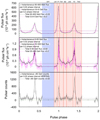 |
Fig. 1. Phaseograms of the Crab pulsar in different energy bands. The > 85 GeV phaseogram observed by VERITAS (bottom panel) is taken from Nguyen & VERITAS Collaboration (2015). |
Comparing all LAT phaseograms presented here, we have no evidence for any phase shift of the two peaks (< 1σ; see Table 1). According to the pulse shapes, we divide the on-pulse region into 7 phase ranges for detailed analyses: Phase 0.88–0.96 (the leading wing of the first pulse; LW1), 0.96–0.02 (the peak region of the first pulse; P1), 0.02–0.12 (the trailing wing of the first pulse; TW1), 0.12–0.20 (the bridge between two pulses; BD), 0.20–0.36 (LW2), 0.36–0.42 (P2) and 0.42–0.58 (TW2).
Pulse peak phases determined from LAT phaseograms.
In 60–600 MeV and 0.6–6 GeV, the ratios of maximum fluxes of P1 to P2 are 2.60 ± 0.05 and 2.85 ± 0.08, respectively. This ratio greatly decreases to 1.54 ± 0.23 in 6–60 GeV and to 1.14 ± 0.59 in 20–500 GeV. It further drops to an even smaller value of 0.57 ± 0.09 in the > 85 GeV band.
From 60–600 MeV to 0.6–6 GeV, the fractional flux of BD increases from (1.82 ± 0.09)% to (3.15 ± 0.07)%. This fraction further rises to (8.38 ± 0.73)%, (4.7 ± 4.4)% and (11.1 ± 4.2)% in 6–60 GeV, 20–500 GeV and > 85 GeV respectively.
3.2. Wavelet analyses on LAT phaseograms
At any photon energy, the flux of the Crab pulsar changes exponentially during the wing phases. In order to investigate the instantaneous rates of flux change at different phases and energies, we apply continuous wavelet transforms to the preliminary LAT phaseograms which have a uniform bin size of a 0.02 phase interval. The Ricker wavelet is adopted. The photon statistics above 20 GeV are not sufficient for the wavelet transform. The results are shown in Fig. 2.
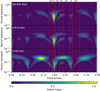 |
Fig. 2. Wavelet maps of the preliminary LAT phaseograms in three exclusive energy bands. A continuous Fourier transform is applied in the period domain for each phaseogram. The Ricker wavelet is adopted. The power index (the colour scale) is defined as the variance per unit period per unit phase divided by the maximum. Each red vertical line is a border between two phase ranges we define. |
The wavelet scale represents the timescale of flux change. Overall, at higher energies, the wavelet components at LW1 and TW2 extend to lower wavelet scales and become closer to vertical, while the components at TW1, LW2 and BD have greater power indices and become more tightly connected with each other.
Considering the pulse profiles and wavelet transformations synthetically, we derive a number of general trends: As the photon energy increases,
(a) the rate of flux increase in LW1 becomes faster, leading to a narrower wing;
(b) the rate of flux decrease in TW1 becomes slower, leading to a broader wing;
(c) the rate of flux increase in LW2 becomes slower, leading to a broader wing;
(d) the rate of flux decrease in TW2 becomes faster, leading to a narrower wing;
(e) the flux ratio of P1 to P2 drops;
(f) the fractional flux of BD rises.
The trends (a), (d) and (e) confirm what was reported in Abdo et al. (2010). In the following sub-sections, we further examine the trends (a)–(f) with spectral analyses.
3.3. LAT SEDs for different pulse phases
3.3.1. Scheme of spectral analyses
In broadband spectral analyses, we enable the energy dispersion correction which operates on the count spectra of most sources including the entire Crab pulsar/nebula complex, following the recommendations of the Fermi Science Support Center. The energy spectrum of the un-pulsed nebular emission in the
60 MeV–100 GeV band is reconstructed by fitting a two-component (additive) model to the data collected during OFF. The flux normalisation of the pulsar component is fixed at 0. Similar to previous studies (Buehler et al. 2012; Yeung & Horns 2020), we assign the synchrotron component a PL with a photon index constrained within 3–5, and assign the IC component a log-parabola (LP):
where α is constrained within 0–2. It turns out that the synchrotron component has a PL index of 3.427 ± 0.019 and an integrated flux of (2.500 ± 0.018)×10−6 ph cm−2 s−1 in the full phase, while the LP parameters of the IC component are determined to be α = 1.759 ± 0.023, β = 0.106 ± 0.014 and N0 = (5.12 ± 0.14)×10−13 cm−2 s−1 MeV−1 (scaled to the full phase).
Then, we apply this nebular model to reconstruct the pulsar spectra at different phases in the same energy band. We examine how well the pulsar spectrum at each phase is described by, respectively, a power law with a super- or sub-exponential cutoff (PLSEC):
![Mathematical equation: $$ \begin{aligned} \frac{\mathrm{d}N}{\mathrm{d}E}=N_0\left(\frac{E}{E_0}\right)^{-\Gamma }\mathrm{exp}\left[-\left(\frac{E}{E_c}\right)^{\lambda }\right] \ , \end{aligned} $$](/articles/aa/full_html/2020/08/aa38166-20/aa38166-20-eq4.gif)
and a power law with an exponential cutoff (PLEC) where λ in PLSEC is fixed at 1. The pulsar parameters are left free while the nebular parameters are fixed at the determined values (with proper scalings to flux normalisations according to phase intervals). The obtained spectral models for the pulsar are tabulated in Table 2. The phase-averaged pulsar spectrum is plotted with the nebular spectrum in Fig. 3, and the phase-resolved pulsar spectra are plotted in Fig. 4. Each presented flux has been scaled by the inverse of the phase interval (i.e. it refers to as the flux per unit phase). The spectral parameters for individual phase bins of 0.04 are plotted in Figs. 5 and 6.
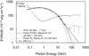 |
Fig. 3. Phase-averaged LAT SEDs of the Crab pulsar and the Crab Nebula. The 4FGL model for the Crab pulsar, reconstructed with fixing λ at 2/3, is overlaid for comparison. All upper limits presented are at a 95% confidence level. We overlay the 60 MeV–100 GeV spectrum predicted by PLSEC and the 10–500 GeV spectrum predicted by PL. |
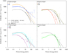 |
Fig. 4. Phase-resolved LAT SEDs of the Crab pulsar. The vertical axis of each panel shows the differential flux per unit phase (δ). All upper limits presented are at a 95% confidence level. For each phase we investigate, we overlay the 60 MeV–100 GeV spectrum predicted by PLSEC and the 10–500 GeV spectrum predicted by PL. The model lines fit to the phase-averaged pulsar spectrum (Fig. 3) are also overlaid on each panel for comparison. Since the Crab pulsar is not significantly detected (< 2σ) above 10 GeV at LW1 and TW2, the upper limits on differential fluxes at these energies and phases are represented by “ad hoc” PL models (the red and purple straight lines appended with arrows), each of which is determined through iterating the prefactor while fixing the index at the maximum-likelihood value. |
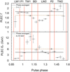 |
Fig. 5. Photon indices Γ and cutoff energies Ec yielded by PLEC for individual phase bins of 0.04. |
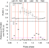 |
Fig. 6. λ values yielded by PLSEC and preference of PLSEC over PLEC for individual phase bins of 0.04. The latter is computed as the square root of the TS difference between those two models. |
60 MeV–100 GeV spectral properties of the Crab pulsar at different phases.
We repeat this chain of exercise for the 10–500 GeV band. For the nebular emission, the synchrotron component is negligible, so we remove it from the source model. The nebular IC component is still modelled as a LP, while the pulsar component is modelled as a PL. The best-fit parameters for the nebula are α = 1.86 ± 0.14, β = 0.023 ± 0.047 and N0 = (5.10 ± 0.42)×10−13 cm−2 s−1 MeV−1 (scaled to the full phase). The results are tabulated in Table 3 and are overlaid in Figs. 3 and 4. We also examine how significant the improvement is when we assign a curved model to the pulsar spectrum. Since the photon index at BD appears to be higher, we adjust the phase width of BD and study the evolution of the photon index (Fig. 7). The narrowest phase width of BD we investigate is 0.05 for which the Crab pulsar is detected at a ∼4σ significance.
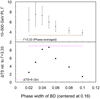 |
Fig. 7. Top: evolution of the 10–500 GeV PL index Γ with adjustments to the phase width of BD. Bottom: corresponding TS differences between fixing Γ at the phase-averaged value of 3.33 and leaving it free. Each of their square roots is the significance at which the local spectrum for an adjusted phase interval of BD is softer than the phase-averaged spectrum. |
10–500 GeV spectral properties of the Crab pulsar at different phases.
We proceed to generate binned spectra for the nebula and pulsar. We divide the 60 MeV–6 GeV band into 12 discrete energy bins (six bins per decade). 6–10 GeV is the 13th bin. The 10–500 GeV band is divided into five discrete bins, the first of which is further split into two. The procedures of broadband fittings are also applied to the spectral fittings of each bin. The nebular emission in each bin is modelled as a PL with an index fixed at a value derived from the broadband fitting. The results are overlaid in Figs. 3 and 4 as well.
Based on the binned spectra, we compute the pulsed fraction of the entire Crab pulsar/nebula complex, as well as the pulsar flux ratios between different pairs of phases at energies from 60 MeV to 100 GeV (plotted in Fig. 8). The pulsed fraction is defined as (Fmax − Fmin)/(Fmax + Fmin), where Fmin is the nebular flux, and Fmax is the pulsar flux in either P1 or P2 (the higher one) added to the nebular flux.
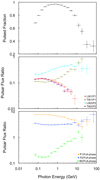 |
Fig. 8. Top: pulsed fraction of the entire Crab pulsar/nebula complex. Middle and bottom: flux ratios of the Crab pulsar between different pairs of phases in different energy bins. We recall that each flux has been scaled by the inverse of the phase interval. |
3.3.2. Summary of spectral properties
The pulsed fraction of the entire Crab pulsar/nebula complex is strongly dependent on the photon energy (see Fig. 8). It is ≳90% (and ≳80%) in 0.2–4 GeV (and 0.1–8 GeV). It drops to 25–50% in 20–100 GeV.
For the phase-averaged pulsar spectrum in 60 MeV–100 GeV, a PLSEC with λ ≈ 0.31 fits the data better than PLEC, indicating that a sub-exponential cutoff is strongly favoured. It is comforting to see that, in 0.2–14 GeV, this PLSEC model agrees within 15% with the 4FGL model reconstructed with fixing λ at 2/3. The λ values are widely varying with the pulse phase (see Fig. 6 and Table 2). Noticeably, during the phase 0.04–0.28, λ is consistent with 1 within the tolerance of statistical uncertainties and PLSEC is not significantly preferred over PLEC (≲1σ). In a PLSEC model, there is a strong correlation of λ with any other parameter, making it nonsensical to compare their values among different phases. Instead, we compare the Γ and Ec values of PLEC models among different phases.
The PLEC model for the full-phase spectrum has a photon index Γ ≈ 1.85 and a cutoff energy Ec = 4.3 ± 0.1 GeV. During the phase 0.08–0.36 (and 0.16–0.28), PLEC fittings yield harder Γ of ≲1.7 (and ∼1.45). During the phase 0.04–0.16 and 0.16–0.24, Ec of PLEC is as high as ∼10.5 GeV and ∼6 GeV, respectively (see Fig. 5). These indicate that the total fractional flux of TW1, BD and LW2 generally increases with the photon energy. As follows, we summarise the < 10 GeV spectral properties of the Crab pulsar based on PLEC and binned spectra (see Figs. 3, 4 and 8 as well as Table 2), and relate them to the trends (a)–(f) derived in Sect. 3.2.
(i) The Γ value at LW1 is lower than that at P1 by 0.07 ± 0.02. On the other hand, the Ec value at LW1 is about 40% of that at P1. The flux ratio of LW1 to P1 is strongly decreasing in 0.5–10 GeV, confirming the trend (a).
(ii) Γ at TW1 and that at P1 are consistent with each other within the tolerance of statistical uncertainties, and Ec at TW1 is three times higher than that at P1. The flux ratio of TW1 to P1 is strongly increasing in 0.5–10 GeV, confirming the trend (b).
(iii) Γ at LW2 is significantly lower than that at P2 by 0.28 ± 0.01. On the other hand, Ec at LW2 is about three-fourth of that at P2. At ∼250 MeV, the flux ratio of LW2 to P2 starts rising with the photon energy significantly. This increment might come to an end at > 4 GeV. Hence, we have strong evidence for the validity of the trend (c) in 0.25–4 GeV.
(iv) Γ at TW2 is consistent with that at P2 (the difference is only at a ∼1.6σ significance), and Ec at TW2 is approximately 30% of that at P2. At ∼350 MeV, the flux ratio of TW2 to P2 starts dropping with the photon energy significantly. This decrement might come to an end at > 2 GeV. Hence, we have strong evidence for the validity of the trend (d) in 0.35–2 GeV.
(v) Both the Γ values at P1 and P2 closely match the one for the full phase (the differences are ≲0.06). Ec at P1 is about two-third of that for the full phase, which is about two-third of that at P2. In 60 MeV–1.5 GeV, the fractional flux of P1 is essentially uniform (the percent variance between any two bins is ≲20%). Above 1.5 GeV, the fractional flux of P1 starts dropping with the photon energy. On the other hand, the fractional flux of P2 remains uniform at energies between 60 MeV and 10 GeV. Hence, the trend (e) is manifested in 1.5–10 GeV.
(vi) BD has the lowest Γ value among all phases we investigate. It is much lower than Γ for the full phase by 0.34 ± 0.03. Also, Ec at BD is higher than that for the full phase by a factor of ∼1.8. The fractional flux of BD is robustly increasing in 0.35–10 GeV, confirming the trend (f).
In 10–500 GeV, a PL is sufficient to describe the pulsar spectrum at each phase, and likelihood ratio tests indicate that any curved models are not statistically required (≲1σ). Therefore, the energy-dependence of a flux ratio between two phases above 10 GeV can be directly inferred from their difference in the photon index (see Table 3). Exceptionally, the detection significance of the Crab pulsar at LW1 and TW2 is too low (< 2σ) so that the “ad hoc” PL models for these two phases cannot precisely predict the pulsar’s differential flux. The photon indices of the Crab pulsar for P1 and TW1 are consistent with each other within the tolerance of statistical uncertainties. The indices for LW2 and P2 are consistent with each other within the tolerance of 1.5σ uncertainties. Therefore, we have no robust evidence for the validities of the trends (a)–(d) at energies above 10 GeV.
Interestingly, while the < 3 GeV spectrum of the Crab pulsar is hardest at BD, its > 10 GeV spectrum is apparently softest at BD. This is consistent with the relatively sharp cutoff of the BD spectrum reported in Table 2. During the phase 0.135–0.185 (a central interval of BD), the fractional flux drops as E−2.6 ± 1.2 at a ∼3σ significance (see Fig. 7), indicating a potential reverse of the trend (f) above 10 GeV. The validity of the trend (e) above 10 GeV is examined in the next sub-section with joint fits of the LAT and ground-based instruments’ spectral points.
3.4. Comparing LAT spectra to observations of ground-based instruments
It is interesting to join the spectral data of LAT and ground-based instruments together for comparisons. Before that, we adjust the phase ranges of the two peaks to be the same as those defined in Ansoldi et al. (2016) (Phase 0.983–0.026 and 0.377–0.422; thereafter P1M and P2M respectively). For these two phase ranges, we follow the same scheme to re-compute the LAT fluxes of the Crab pulsar in different energy bins starting from 10 GeV, which are plotted with the MAGIC fluxes in Fig. 9. For the full-phase, the LAT and VERITAS fluxes of the Crab pulsar at > 10 GeV (the latter is taken from Nguyen & VERITAS Collaboration 2015) are overlaid in Fig. 9 as well.
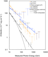 |
Fig. 9. > 10 GeV SEDs of the Crab pulsar at different pulse phases observed with LAT and ground-based instruments. The vertical axis shows the differential flux per unit phase (δ). The horizontal axis shows the measured photon energy (unscaled). Be noted that the orange/blue LAT bins presented here are different from those presented in Fig. 4 because the phase ranges are adjusted for comparison purpose. For each phase we investigate, we overlay the spectrum predicted by the joint-instrument fit of PLSF. The PLSEC fit to the broadband LAT spectrum in the full phase (Fig. 3) and its extrapolation are also overlaid for comparison. |
It is clearly demonstrated that the phase-averaged VERITAS fluxes at energies above 80 GeV are higher than the extrapolated fluxes of the PLSEC fit to the broadband LAT spectrum. Also, for each phase interval we investigate here, a PL is sufficient to describe the spectrum between 10 GeV and ∼1 TeV, and a spectral curvature or break is not statistically required (< 1σ).
In order to take into account the differences in energy scale among LAT, MAGIC and VERITAS, we fitted the data set of each phase to a power law with a scaling factor on photon energies measured by ground-based instruments (PLSF):

Since the data for P1M and P2M is collected by the same ground-based instrument, their data sets are fit together such that their solutions share the same scaling factor ϵ. The results of fittings are presented in Table 4 and the best-fit model lines are overlaid in Fig. 9.
Joint fits of the LAT and ground-based instruments’ spectral points for the Crab pulsar at different phases.
It is worth mentioning that the ϵ values obtained for MAGIC and VERITAS are both ∼1.22. Taking the statistical uncertainties into consideration, they are not significantly larger than 1 (≤1.8σ). It is also comforting to note that the best-fit ϵ − 1 values are only half of a fractional bin width of the ground-based instruments’ data. Therefore, we have obtained physically reasonable fits.
It turns out that the photon index Γ for P1M is lower than that for the full phase by only ∼1.2σ, while Γ for P2M is lower than those for P1M and the full phase by ∼2.1σ and ∼3.6σ respectively. In other words, as the photon energy increases from 10 GeV to ∼1 TeV, the fractional flux of P1 remains constant or even slightly rises back, and that of P2 is significantly rising. The validity of the trend (e) is still suggested at energies > 10 GeV. Since the fluxes of LW1 and TW2 account for a negligibly small fraction of ≤6% (at a 95% confidence level) above 10 GeV, the rise in total fractional flux of P1 and P2 implies a decline in total fractional flux of TW1, BD and LW2. This strengthens the interpretation that the trend (f) is reversed.
4. Discussion and conclusion
Our pulse profiles, wavelet transformations and spectral analyses for the Crab pulsar both demonstrate the strong dependence of the pulse shape on the photon energy, confirming previous studies. Equivalently, the LAT spectral shape of the Crab pulsar widely varies from phase to phase, indicating multiple origins of γ-ray emissions. According to the change in flux proportion among different phases with energy, the trends (a)–(f) derived in Sect. 3.2 are generally valid below 10 GeV.
At any on-pulse phase we investigate, the broadband LAT spectrum of the Crab pulsar exhibits a (sub-)exponential cutoff at Ec ≲ 10 GeV. We observe a higher PLEC cutoff energy at P2 than at P1 for the Crab pulsar. Interestingly, such a trend is predicted to occur for about 75% of cases in the scenario of a dissipative magnetosphere model, where a relatively larger and azimuthally dependent electric field operates outside the light cylinder (Brambilla et al. 2015).
In the framework of Lyutikov (2012) and Lyutikov et al. (2012) for IC emission within the outer gap, the γ-ray spectrum of a pulsar could also manifest itself as a broken power law whose spectral break would correspond to a break in the electron distribution. This prediction is also consistent with a property observed by LAT and ground-based instruments: The Crab pulsar’s spectrum from 10 GeV to ∼1 TeV follows a PL tail.
For the spectrum during the phase 0.04–0.24 (covering the whole BD), λ yielded by PLSEC is ≳1 and Ec yielded by PLEC is ∼(6–10.5) GeV, consistent with an inherent feature (a super-exponential cutoff) predicted in polar cap models (e.g. de Jager 2002; Dyks & Rudak 2004). Such a relatively sharp cutoff is explainable in terms of strong magnetic absorption of low-altitude γ-ray photons above 10 GeV. However, the bridge emission of the Crab pulsar is significantly detected by MAGIC at energies up to 200 GeV (Aleksić et al. 2014). The PL indices of its > 10 GeV LAT spectrum (in this work) and > 50 GeV MAGIC spectrum (Aleksić et al. 2014) are both ∼4. This is not expected in polar cap models.
During LW1, P1, P2, and TW2, a sub-exponential cutoff with λ ≤ 0.6 is strongly favoured to describe the observed spectrum. This rules out the polar cap origin and suggests high-altitude emission zones for these phases. While a traditional outer gap model naturally explains the sub-exponential cutoff detected for the Geminga pulsar (Ahnen et al. 2016), it can only account for the emissions of the Crab pulsar at energies no higher than 10 GeV. The Crab pulsar’s spectrum at each pulse peak exhibits a > 10 GeV PL tail (in this work) which is much harder than that of the Geminga pulsar (Ahnen et al. 2016), and the tail for P2 even extends to 1.5 TeV without a spectral break (Ansoldi et al. 2016). Therefore, a more complicated scenario is required to explain the spectral properties of the Crab pulsar at P1 and P2.
The IC γ-rays (including SSC emission) from magnetospheric acceleration gaps, with “ad hoc” modifications to the models, can roughly match the P1 and P2 fluxes of the Crab pulsar at energies up to 400 GeV (e.g. Aleksić et al. 2011, 2012; Harding & Kalapotharakos 2015; Osmanov & Rieger 2017). Impressively, Harding & Kalapotharakos (2015) took into account the primarily accelerated electrons as well as the leptonic pairs generated by cascades, and Osmanov & Rieger (2017) considered magnetocentrifugal particle acceleration which is efficient close to the light cylinder. Proposed feasible alternatives include wind models, where pulsed γ-rays are due to synchrotron and/or IC radiation from relativistic electrons outside the light cylinder. Aharonian et al. (2012) modelled the pulsed γ-ray emission of the instantaneously accelerated wind, while Arka & Dubus (2013) and Mochol & Petri (2015) modelled that of the wind current sheet.
The trends (a) and (d) of the Crab pulsar entail a decrease in pulse width with increasing energy, which is also detected for the Vela pulsar (DeCesar 2013; H. E. S. S. Collaboration 2018). Such a phenomenon is naturally explained by wind models as well. Besides, a harder spectrum at P2 compared to P1 (i.e. the trend (e)) is observed for both Crab and Vela pulsars (this work; DeCesar 2013; H. E. S. S. Collaboration 2018). This could be attributed to an anisotropy of the wind (Aharonian et al. 2012). Furthermore, wind models predict the bridge emission above 50 GeV as well, but a more complicated density profile of the wind is required to reproduce the observed flux proportion among the bridge and two peaks (Aharonian et al. 2012; Khangulyan et al. 2012).
For the phase-averaged spectrum in GeV–TeV, a schematic comparison of observational results with different theoretical predictions is shown in Fig. 10. Both of the two outer gap models, established by Aleksić et al. (2012) and Harding & Kalapotharakos (2015) respectively, fail to describe the spectral shape observed in 1–10 GeV. The sum of the freshly-accelerated wind’s IC emission modelled by Aharonian et al. (2012) and the extrapolation of our PLSEC model can account for the γ-ray spectrum up to ∼400 GeV. This implies that our PLSEC can be interpreted as a nominal component (i.e. synchro-curvature radiation from the outer gap and/or wind). On the other hand, Mochol & Petri (2015) established a model for a current sheet of striped wind which can, in absence of an outer-gap component, satisfactorily reproduce the observed flux and spectral shape from 1 GeV to 1 TeV. In this model, the transition from the synchrotron-dominated spectrum to the SSC-dominated spectrum occurs at ∼300 GeV.
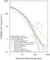 |
Fig. 10. Comparison of the observed full-phase spectrum with four theoretical models, namely OG-A, OG-B, Wind-A and Wind-B. Descriptions of points and lines are at the bottom-left corner. OG stands for “outer gap”. CR stands for “curvature radiation”. “Primary” means emission from primarily accelerated electrons. “Pair” means emission from leptonic pairs generated by cascades. “OG-B (Extended)” is the nominal OG-B model modified with a power-law extension to the cascade pair spectrum. References: [0] this work, [1] Nguyen & VERITAS Collaboration (2015), [2] Ansoldi et al. (2016), [3] Aleksić et al. (2012), [4] Harding & Kalapotharakos (2015), [5] Aharonian et al. (2012), [6] Mochol & Petri (2015). |
All in all, we propose a hybrid scenario where different acceleration sites account for pulsed γ-rays of the Crab pulsar at different phases and energies. Roughly speaking, the polar cap is responsible for the emission at and around the bridge below 10 GeV, the outer gap is responsible for < 10 GeV emissions at other phases, and the wind is responsible for emissions above 10 GeV at any phase. In a more detailed modelling approach, one should carefully deal with the transition phases and transition energies among different emission components.
Acknowledgments
PKHY acknowledges the support of the DFG under the research grant HO 3305/4-1. PKHY gives sincere gratitude to D. Horns for useful discussions and for his encouragement regarding my submission as a single author. We greatly appreciate M. Kerr for providing the ephemeris of the Crab pulsar for phased analysis. We thank D. Carreto Fidalgo for his help in reconstructing Fig. 10. We thank the anonymous referee for very useful comments which helped to improve the manuscript.
References
- Abdo, A. A., Ackermann, M., Ajello, M., et al. 2010, ApJ, 708, 1254 [NASA ADS] [CrossRef] [Google Scholar]
- Abdo, A. A., Ajello, M., Allafort, A., et al. 2013, ApJS, 208, 17 [NASA ADS] [CrossRef] [Google Scholar]
- Aharonian, F. A., & Bogovalov, S. V. 2003, New Astron., 8, 85 [NASA ADS] [CrossRef] [Google Scholar]
- Aharonian, F. A., Bogovalov, S. V., & Khangulyan, D. 2012, Nature, 482, 507 [NASA ADS] [CrossRef] [PubMed] [Google Scholar]
- Ahnen, M. L., Ansoldi, S., Antonelli, L. A., et al. 2016, A&A, 591, A138 [NASA ADS] [CrossRef] [EDP Sciences] [Google Scholar]
- Aleksić, J., Alvarez, E. A., Antonelli, L. A., et al. 2011, ApJ, 742, 43 [NASA ADS] [CrossRef] [Google Scholar]
- Aleksić, J., Alvarez, E. A., Antonelli, L. A., et al. 2012, A&A, 540, A69 [NASA ADS] [CrossRef] [EDP Sciences] [Google Scholar]
- Aleksić, J., Ansoldi, S., Antonelli, L. A., et al. 2014, A&A, 565, L12 [NASA ADS] [CrossRef] [EDP Sciences] [Google Scholar]
- Ansoldi, S., Antonelli, L. A., Antoranz, P., et al. 2016, A&A, 585, A133 [NASA ADS] [CrossRef] [EDP Sciences] [Google Scholar]
- Arka, I., & Dubus, G. 2013, A&A, 550, A101 [NASA ADS] [CrossRef] [EDP Sciences] [Google Scholar]
- Arons, J. 1983, ApJ, 266, 215 [NASA ADS] [CrossRef] [Google Scholar]
- Bogovalov, S. V., & Aharonian, F. A. 2000, MNRAS, 313, 504 [NASA ADS] [CrossRef] [Google Scholar]
- Brambilla, G., Kalapotharakos, C., Harding, A. K., & Kazanas, D. 2015, ApJ, 804, 84 [NASA ADS] [CrossRef] [Google Scholar]
- Buehler, R., Scargle, J. D., Blandford, R. D., et al. 2012, ApJ, 749, 26 [NASA ADS] [CrossRef] [Google Scholar]
- Cheng, K. S., Ho, C., & Ruderman, M. 1986, ApJ, 300, 500 [NASA ADS] [CrossRef] [Google Scholar]
- Cheng, K. S., Ruderman, M., & Zhang, L. 2000, ApJ, 537, 964 [NASA ADS] [CrossRef] [Google Scholar]
- Daugherty, J. K., & Harding, A. K. 1982, ApJ, 252, 337 [NASA ADS] [CrossRef] [Google Scholar]
- DeCesar, M. E. 2013, PhD thesis, University of Maryland, College Park, USA [Google Scholar]
- de Jager, O. C. 2002, Bull. Astron. Soc. India, 30, 85 [Google Scholar]
- Dyks, J., & Rudak, B. 2003, ApJ, 598, 1201 [NASA ADS] [CrossRef] [Google Scholar]
- Dyks, J., & Rudak, B. 2004, Adv. Space Res., 33, 581 [NASA ADS] [CrossRef] [Google Scholar]
- Fermi-LAT Collaboration 2020, ApJS, 247, 33 [NASA ADS] [CrossRef] [Google Scholar]
- Fierro, J. M., Michelson, P. F., Nolan, P. L., & Thompson, D. J. 1998, ApJ, 494, 734 [NASA ADS] [CrossRef] [Google Scholar]
- Harding, A. K., & Kalapotharakos, C. 2015, ApJ, 811, 63 [NASA ADS] [CrossRef] [Google Scholar]
- Harding, A. K., Tademaru, E., & Esposito, L. W. 1978, ApJ, 225, 226 [NASA ADS] [CrossRef] [Google Scholar]
- Harding, A. K., Kalapotharakos, C., Barnard, M., & Venter, C. 2018, ApJ, 869, L18 [NASA ADS] [CrossRef] [Google Scholar]
- H. E. S. S. Collaboration (Abdalla, H., et al.) 2018, A&A, 620, A66 [NASA ADS] [CrossRef] [EDP Sciences] [Google Scholar]
- Khangulyan, D., Aharonian, F. A., & Bogovalov, S. V. 2012, in AIP Conf. Ser., eds. F. A. Aharonian, W. Hofmann, & F. M. Rieger, 1505, 29 [Google Scholar]
- Lobanov, A. P., Horns, D., & Muxlow, T. W. B. 2011, A&A, 533, A10 [NASA ADS] [CrossRef] [EDP Sciences] [Google Scholar]
- Lyutikov, M. 2012, ApJ, 757, 88 [NASA ADS] [CrossRef] [Google Scholar]
- Lyutikov, M., Otte, N., & McCann, A. 2012, ApJ, 754, 33 [NASA ADS] [CrossRef] [Google Scholar]
- Mochol, I., & Petri, J. 2015, MNRAS, 449, L51 [NASA ADS] [CrossRef] [Google Scholar]
- Muslimov, A. G., & Harding, A. K. 2004, ApJ, 606, 1143 [NASA ADS] [CrossRef] [Google Scholar]
- Nguyen, T., & VERITAS Collaboration 2015, Int. Cosmic Ray Conf., 34, 828 [Google Scholar]
- Osmanov, Z., & Rieger, F. M. 2017, MNRAS, 464, 1347 [NASA ADS] [CrossRef] [Google Scholar]
- Romani, R. W. 1996, ApJ, 470, 469 [NASA ADS] [CrossRef] [Google Scholar]
- Romani, R. W., & Yadigaroglu, I. A. 1995, ApJ, 438, 314 [NASA ADS] [CrossRef] [Google Scholar]
- Sturrock, P. A. 1971, ApJ, 164, 529 [NASA ADS] [CrossRef] [Google Scholar]
- Takata, J., Shibata, S., Hirotani, K., & Chang, H. K. 2006, MNRAS, 366, 1310 [NASA ADS] [CrossRef] [Google Scholar]
- Tang, A. P. S., Takata, J., Jia, J. J., & Cheng, K. S. 2008, ApJ, 676, 562 [NASA ADS] [CrossRef] [Google Scholar]
- VERITAS Collaboration (Aliu, E., et al.) 2011, Science, 334, 69 [NASA ADS] [CrossRef] [PubMed] [Google Scholar]
- Yeung, P. K. H., & Horns, D. 2020, A&A, 638, A147 [CrossRef] [EDP Sciences] [Google Scholar]
All Tables
Joint fits of the LAT and ground-based instruments’ spectral points for the Crab pulsar at different phases.
All Figures
|
Fig. 1. Phaseograms of the Crab pulsar in different energy bands. The > 85 GeV phaseogram observed by VERITAS (bottom panel) is taken from Nguyen & VERITAS Collaboration (2015). |
| In the text | |
|
Fig. 2. Wavelet maps of the preliminary LAT phaseograms in three exclusive energy bands. A continuous Fourier transform is applied in the period domain for each phaseogram. The Ricker wavelet is adopted. The power index (the colour scale) is defined as the variance per unit period per unit phase divided by the maximum. Each red vertical line is a border between two phase ranges we define. |
| In the text | |
|
Fig. 3. Phase-averaged LAT SEDs of the Crab pulsar and the Crab Nebula. The 4FGL model for the Crab pulsar, reconstructed with fixing λ at 2/3, is overlaid for comparison. All upper limits presented are at a 95% confidence level. We overlay the 60 MeV–100 GeV spectrum predicted by PLSEC and the 10–500 GeV spectrum predicted by PL. |
| In the text | |
|
Fig. 4. Phase-resolved LAT SEDs of the Crab pulsar. The vertical axis of each panel shows the differential flux per unit phase (δ). All upper limits presented are at a 95% confidence level. For each phase we investigate, we overlay the 60 MeV–100 GeV spectrum predicted by PLSEC and the 10–500 GeV spectrum predicted by PL. The model lines fit to the phase-averaged pulsar spectrum (Fig. 3) are also overlaid on each panel for comparison. Since the Crab pulsar is not significantly detected (< 2σ) above 10 GeV at LW1 and TW2, the upper limits on differential fluxes at these energies and phases are represented by “ad hoc” PL models (the red and purple straight lines appended with arrows), each of which is determined through iterating the prefactor while fixing the index at the maximum-likelihood value. |
| In the text | |
|
Fig. 5. Photon indices Γ and cutoff energies Ec yielded by PLEC for individual phase bins of 0.04. |
| In the text | |
|
Fig. 6. λ values yielded by PLSEC and preference of PLSEC over PLEC for individual phase bins of 0.04. The latter is computed as the square root of the TS difference between those two models. |
| In the text | |
|
Fig. 7. Top: evolution of the 10–500 GeV PL index Γ with adjustments to the phase width of BD. Bottom: corresponding TS differences between fixing Γ at the phase-averaged value of 3.33 and leaving it free. Each of their square roots is the significance at which the local spectrum for an adjusted phase interval of BD is softer than the phase-averaged spectrum. |
| In the text | |
|
Fig. 8. Top: pulsed fraction of the entire Crab pulsar/nebula complex. Middle and bottom: flux ratios of the Crab pulsar between different pairs of phases in different energy bins. We recall that each flux has been scaled by the inverse of the phase interval. |
| In the text | |
|
Fig. 9. > 10 GeV SEDs of the Crab pulsar at different pulse phases observed with LAT and ground-based instruments. The vertical axis shows the differential flux per unit phase (δ). The horizontal axis shows the measured photon energy (unscaled). Be noted that the orange/blue LAT bins presented here are different from those presented in Fig. 4 because the phase ranges are adjusted for comparison purpose. For each phase we investigate, we overlay the spectrum predicted by the joint-instrument fit of PLSF. The PLSEC fit to the broadband LAT spectrum in the full phase (Fig. 3) and its extrapolation are also overlaid for comparison. |
| In the text | |
|
Fig. 10. Comparison of the observed full-phase spectrum with four theoretical models, namely OG-A, OG-B, Wind-A and Wind-B. Descriptions of points and lines are at the bottom-left corner. OG stands for “outer gap”. CR stands for “curvature radiation”. “Primary” means emission from primarily accelerated electrons. “Pair” means emission from leptonic pairs generated by cascades. “OG-B (Extended)” is the nominal OG-B model modified with a power-law extension to the cascade pair spectrum. References: [0] this work, [1] Nguyen & VERITAS Collaboration (2015), [2] Ansoldi et al. (2016), [3] Aleksić et al. (2012), [4] Harding & Kalapotharakos (2015), [5] Aharonian et al. (2012), [6] Mochol & Petri (2015). |
| In the text | |
Current usage metrics show cumulative count of Article Views (full-text article views including HTML views, PDF and ePub downloads, according to the available data) and Abstracts Views on Vision4Press platform.
Data correspond to usage on the plateform after 2015. The current usage metrics is available 48-96 hours after online publication and is updated daily on week days.
Initial download of the metrics may take a while.