| Issue |
A&A
Volume 640, August 2020
|
|
|---|---|---|
| Article Number | A22 | |
| Number of page(s) | 9 | |
| Section | Extragalactic astronomy | |
| DOI | https://doi.org/10.1051/0004-6361/202037759 | |
| Published online | 04 August 2020 | |
GASP
XXVI. HI gas in jellyfish galaxies: The case of JO201 and JO206⋆
1
Department of Physics and Electronics, Rhodes University, PO Box 94, Makhanda 6140, South Africa
e-mail: This email address is being protected from spambots. You need JavaScript enabled to view it.
2
INAF-Osservatorio Astronomico di Cagliari, Via della Scienza 5, 09047 Selargius, CA, Italy
3
INAF-Osservatorio Astronomico di Padova, Vicolo dell’Osservatorio 5, 35122 Padova, Italy
4
Kapteyn Astronomical Institute, University of Groningen, Landleven 12, 9747 AV Groningen, The Netherlands
5
Department of Astronomy, Columbia University, Mail Code 5246, 550 W 120th Street, New York, NY 10027, USA
6
Instituto de Física y Astronomía, Universidad de Valparaíso, Avda. Gran Bretana 1111, Valparaíso, Chile
7
Center for Computational Astrophysics, Flatiron Institute, 162 5th Ave, New York, NY 10010, USA
8
South African Radio Astronomy Observatory, 2 Fir Street, Black River Park, Observatory 7925, South Africa
9
Argelander-Institut fur Astronomie, Auf dem Hugel 71, 53121 Bonn, Germany
10
National Centre for Radio Astrophysics, Tata Institute of Fundamental Research, Postbag 3, Ganeshkhind, Pune 411 007, India
11
ASTRON, Netherlands Institute for Radio Astronomy, Oude Hoogeveensedijk 4, 7991 PD Dwingeloo, The Netherlands
12
Department of Astronomy, University of Cape Town, Private Bag X3, Rondebosch 7701, South Africa
13
Department of Physics, University of Pretoria, Hatfield, Pretoria 0028, South Africa
14
Ruhr University Bochum, Faculty of Physics and Astronomy, Astronomical Institute, 44780 Bochum, Germany
15
Dipartimento di Fisica e Astronomia “Galileo Galilei”, Università di Padova, Vicolo dell’Osservatorio 3, 35122 Padova, Italy
Received:
18
February
2020
Accepted:
2
June
2020
Abstract
We present atomic hydrogen (H I) observations with the Jansky Very Large Array of one of the jellyfish galaxies in the GAs Stripping Phenomena sample, JO201. This massive galaxy (M* = 3.5 × 10¹⁰ M⊙) is falling along the line-of-sight towards the centre of a rich cluster (M200 ∼ 1.6 × 10¹⁵ M⊙, σcl ∼ 982 ± 55 km s−1) at a high velocity ≥3363 km s−1. Its Hα emission shows a ∼40 kpc tail, which is closely confined to its stellar disc and a ∼100 kpc tail extending further out. We find that H I emission only coincides with the shorter clumpy Hα tail, while no H I emission is detected along the ∼100 kpc Hα tail. In total, we measured an H I mass of MHI = 1.65 × 10⁹ M⊙, which is about 60% lower than expected based on its stellar mass and stellar surface density. We compared JO201 to another jellyfish in the GASP sample, JO206 (of a similar mass but living in a ten times less massive cluster), and we find that they are similarly H I-deficient. Of the total H I mass in JO201, about 30% lies outside the galaxy disc in projection. This H I fraction is probably a lower limit since the velocity distribution shows that most of the H I is redshifted relative to the stellar disc and could be outside the disc. The global star formation rate (SFR) analysis of JO201 suggests an enhanced star formation for its observed H I content. The observed SFR would be expected if JO201 had ten times its current H I mass. The disc is the main contributor of the high star formation efficiency at a given H I gas density for both galaxies, but their tails also show higher star formation efficiencies compared to the outer regions of field galaxies. Generally, we find that JO201 and JO206 are similar based on their H I content, stellar mass, and star formation rate. This finding is unexpected considering their different environments. A toy model comparing the ram pressure of the intracluster medium (ICM) versus the restoring forces of these galaxies suggests that the ram pressure strength exerted on them could be comparable if we consider their 3D orbital velocities and radial distances relative to the clusters.
Key words: galaxies: star formation / galaxies: clusters: intracluster medium / radio lines: galaxies
The cubelet containing the galaxy of interest for the paper, J201 is only available at the CDS via anonymous ftp to cdsarc.u-strasbg.fr (130.79.128.5) or via http://cdsarc.u-strasbg.fr/viz-bin/cat/J/A+A/640/A22
© ESO 2020
1. Introduction
In the dense environment of galaxy clusters, the hydrodynamical interaction between galaxies’ interstellar medium (ISM) and the intracluster medium (ICM) plays a key role in transforming galaxies from late types to early types. Among the several types of interactions discussed in the literature (e.g. Gunn & Gott 1972; Cowie & Songaila 1977; Nulsen 1982), the ram pressure exerted by the ICM on galaxies’ ISM can be very efficient at removing gas from galaxies as well as affecting their star formation activity. The degree of this effect may vary depending on the strength of the ram pressure exerted on a galaxy and its physical properties.
In some cases, the diffuse atomic hydrogen (H I) gas is only partially removed or displaced from the stellar disc (Boselli et al. 1997; Vollmer et al. 2001; Chung et al. 2009; Scott et al. 2010; Steinhauser et al. 2016). However, the dense molecular gas cloud may remain unperturbed after the diffuse gas has been stripped and continue to form stars at a low rate. In this case, the star formation (SF) essentially stops as soon as molecular gas is consumed and not replenished (Abramson & Kenney 2014).
In other cases, the ram pressure is so severe (e.g. Jaffe et al. 2018; Quilis et al. 2000) that galaxies are often observed to be H I gas deficient and exhibit asymmetric morphologies (e.g. Boselli & Gavazzi 2006; Fumagalli et al. 2014; McPartland et al. 2016; Gavazzi et al. 2018). These galaxies sometimes show an increased star formation rate even to the point of becoming temporarily brighter than the bright central galaxies of their host clusters (e.g. Owen et al. 2006; Cortese et al. 2007; Owers et al. 2012; Ebeling et al. 2014; George et al. 2018; Vulcani et al. 2018). This implies that the compression of the ISM could possibly induce starbusts.
Moreover, the stripped gas may form knots of star formation in the wake of the galaxy. Examples of these types of cases have been observed in the so called “jellyfish” galaxies (e.g. Yoshida et al. 2008; Hester et al. 2010; Yagi et al. 2010; Fumagalli et al. 2014; Boselli et al. 2016; Fossati et al. 2016; Poggianti et al. 2019; Cramer et al. 2019). The stripped tails of some of these galaxies are detected in Hα and Ultraviolet (UV) (Cortese et al. 2006; Sun et al. 2007; Kenney et al. 2008; Smith et al. 2010; Ebeling et al. 2014; George et al. 2018).
Detailed observations of these galaxies, which include their gaseous tails, are important to gain a full understanding of the ram pressure effect on the star formation efficiency of jellyfish galaxies. While some studies have shown that these galaxies show an overall enhanced SF (e.g. Boissier et al. 2012; Vulcani et al. 2018; Ramatsoku et al. 2019), others find a reduced star formation due to ram pressure stripping (Vollmer et al. 2012; Jachym et al. 2014; Verdugo et al. 2015).
These reports make it imperative to gather large multi-wavelength samples and to conduct detailed studies of these objects (jellyfish galaxies) that are undergoing a transformation in the galaxy cluster environments. The GAs Stripping Phenomena survey (GASP; Poggianti et al. 2017a) has been performed in an effort to conduct this type of a study. Through GASP, a statistically significant sample of jellyfish galaxies has been compiled in nearby clusters (z = 0.04 − 0.07) from the WIde-field Nearby Galaxy-cluster Survey (WINGS; Fasano et al. 2006) and OmegaWINGS (Cava et al. 2009; Varela et al. 2009; Gullieuszik et al. 2015; Moretti et al. 2017). The current GASP operational definition of a jellyfish galaxy is one that exhibits a one-sided tail of debris material whose Hα emission has a length comparable or greater to the diameter of the stellar disc. The optically selected jellyfish candidates were observed with the Multi Unit Spectroscopic Explorer (MUSE) Integral Field spectrograph on the Very Large Telescope (VLT) (Poggianti et al. 2016). This sample covers a wide range of jellyfish morphological asymmetries and masses in different environments. Within the GASP context, the aim is to understand the evolution of the distribution and efficiency of star formation in ram pressure stripped galaxies by studying all phases of the gas in relation to the stellar population properties of these galaxies.
The large radial distribution of the H I gas in galaxies and its sensitivity to mild ram pressures makes it an excellent tracer of gas removal processes in cluster environments (Haynes et al. 1984; Bravo-Alfaro et al. 1997; Gavazzi et al. 2008; Kapferer et al. 2009; Chung et al. 2009; Abramson et al. 2011; Jaffé et al. 2015; Yoon et al. 2017). Therefore to fully understand the physics and the effect of ram pressure stripping on the GASP galaxy sample it is necessary to examine the H I content and distribution. This is what the work presented in this paper focuses on.
We have conducted a follow up on a few GASP galaxies with the Jansky Very Large Array (JVLA; Perley et al. 2009) to study their H I properties. Deb et al. (2020) investigated whether ram pressure stripping might be triggering the Active Galactic Nucleus (AGN) in JO204 by funnelling H I towards the centre of the galaxy. In Ramatsoku et al. (2019) we examined the H I gas stripping and star formation activity of JO206, which resides in the poor galaxy cluster, IIZw108 (M200 ∼ 2 × 10¹⁴ M⊙σcl ∼ 575 ± 33 km s−1; Biviano et al. 2017). We found that the star formation efficiency was higher in JO206 than in galaxies with similar stellar and H I mass.
In this paper we present a study of the neutral gas phase of the jellyfish galaxy, JO201 (αJ2000, δJ2000 = 00:41:30.30, −09:15:45.98; Gullieuszik et al. 2015). This galaxy resides within the rich galaxy cluster, Abell 85 located at a redshift of z = 0.05586 (Moretti et al. 2017). JO201 is undergoing ram pressure stripping along the line of sight in this cluster and exhibits a one-sided tail of stripped material seen at the optical wavelength (Poggianti et al. 2016; Bellhouse et al. 2017, 2019). For this study we aim to compare and contrast the H I properties and star formation activities of these two galaxies in consideration of their different environments.
The paper is organised as follows; in Sect. 2 we give a summary of the properties of JO201 as well as an overview of the available multiwavelength observations. We outline how the H I observations and data reduction were conducted for JO201 in Sect. 3. In Sect. 4 we discuss the H I distribution compared to the Hα of this galaxy. We compare the H I-deficiencies, global and resolved star formation rates as well as the environments of JO201 with those of JO206 in Sect. 5. All the analyses and discussions are summarised in Sect. 6.
Throughout this paper we adopt a Chabrier (2003) initial mass function (IMF) and assume a Λ cold dark matter cosmology with ΩM = 0.3, ΛΩ = 0.7 and a Hubble constant, H0 = 70 km s−1 Mpc−1 .
2. Properties of the JO201 galaxy
JO201, is a spiral galaxy with an AGN at its centre (Poggianti et al. 2017b; Radovich et al. 2019) and a stellar mass of 3.6 × 10¹⁰ M⊙ (Vulcani et al. 2018). It is located within the massive and dynamically complex galaxy cluster, Abell 85 (A 85) in the WINGS/OmegaWINGS sample (Fasano et al. 2006; Cava et al. 2009; Varela et al. 2009; Gullieuszik et al. 2015; Moretti et al. 2017). A 85 has a total mass of M200 ∼ 1.6 × 10¹⁵ M⊙ and a velocity dispersion of σcl ∼ 982 ± 55 km s−1 (Moretti et al. 2017). Within this cluster, JO201 lies at a projected radial distance of 360 kpc from the central brightest cluster galaxy and has a particularly high line-of-sight velocity of about 3.4σcl relative to the cluster’s systemic velocity (Bellhouse et al. 2017).
JO201 is experiencing ram pressure stripping due to the ICM of A 85 (Bellhouse et al. 2017). Its effect is manifested in the form of two long one-sided tails visible in Hα within the GASP survey and debris material as seen at optical wavelengths in the WINGS/OmegaWINGS surveys (Varela et al. 2009; Gullieuszik et al. 2015; Moretti et al. 2017). Bellhouse et al. (2017) performed a quantitative analysis of the strength of ram pressure exerted on JO201 by the ICM of A 85 using the Gunn & Gott (1972) description (Pram = ρICMv2), and calculated a ram pressure strength of Pram = 2.7 × 10⁻¹¹ Nm−2 at the projected distance of the galaxy from the cluster centre. The exerted ram pressure was then compared to its anchoring force, suggesting that more than 40% of the total gas (estimated from Hα) had been removed through ram pressure stripping (see Bellhouse et al. 2017, 2019 for the full analysis).
Although this galaxy has lost about half of its gas due to ram pressure stripping, it is still forming new stars as inferred from its Hα MUSE data, UV imaging from GALEX and ASTROSAT, and CO data from APEX (Bellhouse et al. 2019; George et al. 2018; Venkatapathy et al. 2017; Moretti et al. 2018). These data are illustrated in Fig. 1. The total SFR estimated from the Hα emission after masking the AGN and correcting for stellar absorption and dust extinction1 as in Poggianti et al. (2017a), is 6.1 M⊙ yr−1 (Vulcani et al. 2018).
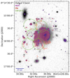 |
Fig. 1. A multiwavelength composite image illustrating all the data available for JO201. The NUV data is shown in violet overlaid on an optical V-band image in grayscale from WINGS. In red we overlay the Hα emission from MUSE. The 12CO(2–1) observations are illustrated by the approximate FWHM of the APEX beam. |
An analysis of the star formation history shows that the stellar disc has stars of all ages, while the stripped tail only comprises young stars formed < 6 × 10⁸ years ago (see Fig. 9 by Bellhouse et al. 2019). These young stars have likely formed in-situ out of the ram pressure stripped ISM, thus strongly implying the presence of cold gas and, therefore, H I both in the tail and disc. This measurement motivated the H I observations described in Sect. 3.
3. HI observations and data processing
The H I data were obtained from observations with the JVLA, project code VLA/17A-293 (PI: B. Poggianti). JO201 was observed in July 2017 for a total of 16 h on source and 4 h on calibrators. The observations were conducted in the C-configuration resulting in an angular resolution of ∼15″. They covered a total bandwidth of 32 MHz, centred at 1360.2103 MHz, which was divided into 1024 channels of width 31.25 kHz each (6.56 km s−1 for H I at z = 0).
The uv-data were processed using the CARACAL pipeline2 which is currently being developed. Using this pipeline we followed the same data reduction steps outlined in Ramatsoku et al. (2019). As a brief summary, an H I data cube with a field of view of 0.7 deg2 was produced using a pixel scale of 5″ with natural weighting (Briggs robustness parameter = 2). We chose this weighting scheme to optimise surface-brightness sensitivity. The resulting H I cube has a Gaussian restoring Point Spread Function (PSF) Full Width at Half Maximum (FWHM) of 16″ × 25″ and a position angle (PA) of 174°. The rms noise level is σ ≈ 0.37 mJy beam−1 per 6.56 km s−1-wide channel. The observational setup and noise level results in an H I column density sensitivity of 4 × 10¹⁹ atoms cm−2 (3σ over a line width of 30 km s−1). For a detailed description of the H I data reduction see Ramatsoku et al. (2019).
4. The distribution of H I in JO201 and comparison with Hα
The H I-line emission of JO201 was extracted from the image cube using SoFiA (Serra et al. 2015). Within the SoFiA H I extraction mask we measure a total H I mass of MHI = 1.65 × 10⁹ M⊙, assuming the galaxy is at the redshift of the cluster, z = 0.05586, D = 239 Mpc (Moretti et al. 2017).
The left panel of Fig. 2 shows the spatial distribution of the H I emission in JO201. The blue contours are from the H I intensity map (i.e. moment 0). They are overlaid on an optical V-band image from WINGS/OmegaWINGS. The red contour outlines the stellar disc defined from the MUSE image using the continuum at the Hα wavelength, with the isophote fit at surface brightness of 1σ above the average sky background level.
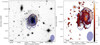 |
Fig. 2. Left panel: VLA H I column density contours overlaid on the V-band image of JO201 from WINGS. Contour levels are drawn at column densities of 4, 8, 12, ... × 1019 atoms cm−2. The FWHM beam size of 16″ × 25″ is indicated by the blue ellipse. The red contours represent the stellar disc and the black contour is the H I disc (see text for a definition). Right panel: Hα emission with H I column density contours (same levels as the left panel) overlaid. The red opaque patch is the stellar disc and the black contour is the H I disc. The black circle is the region over which we estimate the H I flux density as described in the text. |
The black contour represents the expected H I disc size if all the detected H I were distributed on a regular disc and followed standard H I scaling relations. We calculated its size at the 4 × 10¹⁹ atoms cm−2 H I column density sensitivity of our JVLA data taking into account the inclination angle derived from the stars following the methods described in Ramatsoku et al. (2019). To make this calculation we exploited the tight correlation between H I diameters and masses which is parametrised as log(DHI/kpc) = 0.51 log(MHI/M⊙)−3.32, where the H I diameter, DHI is defined at the H I surface density of 1 M⊙ pc−2 (column density 1.25 × 10²⁰ atoms cm−2; Wang et al. 2016). From this relation we compute an H I diameter of DHI = 23 kpc for the unperturbed JO201 model. We then used the Martinsson et al. (2016) H I profile formulation,  to determine the radial surface density. In this formula RΣ,max and σΣ are fixed to 0.2DHI and 0.18DHI, respectively. The free parameter is
  , which we set to 0.4 M⊙ pc−2 such that ΣHI(DHI/2) = 1 M⊙ pc−2. With the above correlations and assuming the H I observational conditions of JO201 (see Sect. 3) we used the 3D-BAROLO package (Di Teodoro & Fraternali 2015) to project the unperturbed H I distribution of JO201 onto the sky with the correct inclination and PA.
The model H I disc has a radius of 24.6 kpc at the 4 × 10¹⁹ atoms cm−2 H I column density sensitivity of our data as shown in the left panel of Fig. 2. We note that for JO201, the stellar and H I disc are similar, therefore throughout the paper we do not differentiate between the two, unless stated otherwise.
We used the projected radius derived from the model (i.e. 24.6 kpc) as a divider between inner (disc) and outer galaxy regions, and find that of the total H I mass measured 1.22 × 10⁹ M⊙ is inside the galaxy disc with ∼0.43 × 10⁹ M⊙ (26%) lying in the outer regions in projection. Below we revisit this analysis based on the velocity distribution as well.
The projected spatial distribution of the H I and Hα show moderately different distributions (e.g. Fig. 2, right panel). H I overlaps almost entirely with the Hα emission within the galaxy disc. It also has a minor offset of ∼5 kpc from the optical centroid in the direction of the stripped tail and shows a compression on the west side of the emission which is also seen in Hα. All these features are hallmarks of ram pressure stripping which we are seeing manifest in the H I distribution. Both the one-sided compression to the west and the bulk offset towards east suggest that the motion of JO201 within A 85 might have a non-negligible component on the plane of the sky. Outside the galaxy disc, the overlap between H I and Hα tail is only seen along the shorter clumpy Hα tail that is closely confined to the disc on the east side.
The non-detection of H I along the outer Hα tail might be due to the small size of the gas clumps (at least judging from the Hα image) compared to the H I PSF. As an example, let us consider the brightest Hα blob of the outer tail (black circle in the right panel of Fig. 2) and test whether it would be detectable in our H I cube. We generously assume that the H I surface density inside this 5 kpc-diameter blob is 5 M⊙ pc−2, which is a typical value of the disc of spiral galaxies but is, in fact, quite high for extraplanar H I (see top-left panel of Fig. 8 in Bigiel et al. 2008). We further assume that the entire H I signal is spread over a velocity interval of 50 km s−1 (twice the typical FWHM of the H I line). With these assumptions, and given the 239 Mpc distance of JO201, the H I flux density of the blob would be 0.14 mJy beam−1. This is equal to a 1σ level when smoothing our H I cube to a channel width of 50 km s−1 in order to match the width of the assumed H I signal. Despite our generous assumptions, the blob would thus not be detectable in our data. Therefore, while we can rule out the presence of an extended (i.e. resolved by our H I PSF) distribution of H I in the outer Hα tail down to 4 × 10¹⁹ atoms cm−2, we cannot rule out that some of the Hα clumps much smaller than our H I PSF contain H I with relatively high column density.
From the projected spatial distribution image it appears as though most of the detected H I lies within the galaxy disc. However, in previous studies Bellhouse et al. (2017) analysed the kinematics of JO201 using MUSE data. In this work they reported that the galaxy had a smooth stellar disc with a co-rotating ionised Hα gas within the inner 6 kpc. However this stars-gas co-rotation is not seen in the outer stellar disc > 6 kpc. In these outer regions they found that the Hα gas trails behind the undisturbed stellar disc due to the line-of-sight ram pressure stripping nature of this galaxy. In the tail (outside of the disc) the stellar kinematics can only be measured very close to the disc (and is decoupled from the gas, that is trailing behind), while further out in the tail there is no stellar disc to compare with. Here we use the position-velocity diagram (PVD) in Fig. 3 to examine the H I gas kinematics and its relation to the stellar disc and Hα emission. From this plot we find that as already reported (Bellhouse et al. 2017), Hα is redshifted with respect to the systemic velocity. This displacement becomes more severe when we examine the H I velocity distribution. In fact the H I emission does not cross the systemic velocity at all. It appears that in addition to the already known east-west asymmetry (most of the H I is to the east of the galaxy), there is also a clear velocity asymmetry. From these PVDs we deduce that it is possible that most of the H I we detect is already outside of the disc – contrary to what we see from the projected spatial distribution (e.g. Fig. 2). The star-H I velocity offset is ≳100 km s−1, taking into account the marginal inclination correction of 1/sin(54 ° ). At this velocity offset it is possible for the H I gas to be lifted above the stellar disc, which typically has scale heights of a few 100 pc, because the gas can travel a distance of ∼1 kpc in a short time-scale of ∼10 Myr. This velocity offset therefore implies that much of the H I we see might already be stripped and is part of the tail.
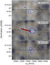 |
Fig. 3. Position velocity diagrams (PVDs) extracted from the H I cube along the three 1.25′ wide right ascension slices indicated in the top right corner. The Hα emission convolved with the H I PSF is shown in orange. For reference, the red contour in the middle panel represents the stellar velocities extracted from Bellhouse et al. (2017) (no convolution to the HI angular resolution was performed). The Hα contours are drawn at surface brightness levels of 1 × 10n erg s−1 cm2 where n = −10, −9, −8 ⋯. The blue contours are the H I emission from the cube drawn at flux densities of 0.3, 0.4, 0.5 ... mJy beam−1 and the negative H I contours are drawn at −0.3, −0.2 ... mJy beam−1. The vertical dashed line is the systemic velocity of the galaxy and the horizontal line is the optical centre. Velocities in the PVDs are in the optical definition using the barycentric standard-of-rest. |
In addition to the Hα and H I distribution, we also examined H I in relation to the star formation rate surface density (ΣSFR) of JO201 as shown in Fig. 4. We find a good agreement between peak ΣSFR and H I emission predominately in the projected disc of JO201. There is also a coincidence between the short H I tails outside the galaxy disc and knots of high ΣSFR in those regions.
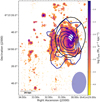 |
Fig. 4. Star formation rate density map (Bellhouse et al. 2019) with H I emission contours overlaid. The contours are at H I column density levels of 4, 8, 12, ... × 1019 atoms cm−2. The FWHM beam size of 25″ × 16″ is shown by the blue ellipse. |
5. HI deficiency and SFR enhancement: JO201 and JO206
In this section we are going to compare the H I gas and star formation properties of JO201 with those of the other jellyfish galaxy with H I data, JO206 in the GASP sample. JO206 is a massive galaxy with a stellar mass, M* = 8.5 × 10¹⁰ M⊙. It lies at a redshift of z = 0.0513, near the centre of the low-mass (M200 ∼ 2 × 10¹⁴ M⊙) galaxy cluster IIZw108 with a velocity dispersion of σ ∼ 575 km s−1. This galaxy is characterised by a long tail (≥90 kpc) of ionised gas stripped away by ram pressure. In Ramatsoku et al. (2019) we analysed the H I gas phase of JO206 and found a similarly long H I tail extending in the same direction as the Hα tail. Its total H I mass is 3.2 × 10⁹ M⊙, of which 1.8 × 10⁹ M⊙ (about 60%) is in the stripped tail (see Fig. 3 in Ramatsoku et al. 2019).
5.1. JO201 and JO206 HI deficiencies
From the morphology of the H I spatial distribution of JO201, it is evident that ram pressure stripping has affected the H I content of this galaxy. A large fraction of the currently detected H I is outside the disc, either in projection on the sky or in velocity (Sect. 4). It is thus possible that JO201 used to have even more H I, which is no longer detectable. Here we compute whether the total detected H I mass of JO201 is significantly less than expected based on known H I scaling relations and compare it with that of JO206. We do so using the scaling relations by Brown et al. (2015) obtained from spectral stacking of ALFALFA data.
Figure 5 shows the scaling between H I fraction MHI/M* and stellar mass M* for galaxies in the Brown et al. (2015) sample with a stellar surface mass density μ* within a factor of 4 of the values measured for JO201 and JO206. This factor is comparable to the uncertainty in the μ* values. JO201 with its μ* = 1.8 × 10⁸ M⊙ kpc−2 (log μ* = 8.3) stellar surface density is represented by the green asterisks while JO206 with μ* = 4.2 × 10⁸ M⊙ kpc−2 (log μ* = 8.6) is denoted in blue.
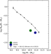 |
Fig. 5. Average stacked H I fraction as function of the stellar mass (Brown et al. 2015). The relation is separated into galaxies with stellar surface brightness comparable to that of JO201 and JO206 within a factor of 4. The scatter in the mass bins is illustrate by the error bars. JO201 is represented by the green asterisk and JO206 by the blue asterisk. |
Compared to the control sample, JO201 is approximately 0.4 dex below the average H I fraction. From the scaling relation the expected H I mass for this galaxy is about 4.13 × 10⁹ M⊙ which indicates that JO201 is missing ∼60% of its H I mass and is therefore H I deficient. This gas mass loss is comparable to that measured based on instantaneous ram pressure description in Bellhouse et al. (2017). It is also similar to the H I gas mass loss of JO206 which is 0.3 dex below the average H I fraction resulting in ∼50% H I deficiency.
We also determined the H I deficiency of these galaxies using the parameter, DefHI = ⟨log MHI(D, T)⟩ − log MHI(D, T)obs (Haynes et al. 1984), which defines the H I-deficiency as the logarithmic difference between the observed H I content and the expected value in isolated galaxies of the same linear size and morphology. The respective morphologies of JO201 and JO206 are Sa-Sab and Sb-Sbc (Fasano et al. 2012) and their R25 radii in the B-band are 17.9″ and 24.95″. With this information we calculate DefHI = 0.44 for JO201 and 0.41 for JO206. The deficiencies of this order (about a factor of 2) are comparable with those we reported from the H I scaling relation. However, we note that they are somewhat within the scatter of typical H I scaling relations. Thus it is possible (although not necessary) that most of the H I originally present in these galaxies is still detectable within or close to the galaxy.
5.2. Global star formation activity
We investigate how the gas loss discussed in the previous section may have affected the global star formation activity of JO201, and how this compares to JO206. We begin by preparing a control sample of field galaxies with the same stellar mass as JO201 and JO206 obtained from the GALEX Arecibo SDSS Survey (GASS; Catinella et al. 2010). We also collected a sample of galaxies from The H I Nearby Galaxy Survey (THINGS; Bigiel et al. 2008, 2010) which we use in Sect. 5.3 to investigate the spatially resolved H I−SFR relation. In Fig. 6 we show the global H I−SFR scaling relation for the GASS sample (Saintonge et al. 2016; see also Doyle & Drinkwater 2006; Huang et al. 2012)
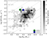 |
Fig. 6. H I−SFR scaling relation showing the star formation rate vs H I mass for galaxies with the same stellar masses as JO201 and JO206. Grey hexagons are galaxies from the control sample (GASS) and the green and blue asterisk represent the JO201 and JO206 galaxies, respectively. The dotted lines indicate the fixed H I depletion times in yr. |
JO201 (SFR = 6.1 M⊙ yr−1) is located approximately 0.6 dex above the average M(H I)–SFR relation similarly to JO206 (SFR = 5.6 M⊙ yr−1). Both galaxies lie at the edge of the distribution of the control sample, and appear to have a higher star formation rate than galaxies of similar stellar mass given their observed H I mass. We note however, that as shown in Fig. 6 there is a large uncertainty associated with the exact SFR enhancement due the large scatter of this H I–SFR scaling relation (see Saintonge et al. 2016). Nevertheless similarly to JO206, we argue that the fact that JO201 is located close to the edge of this distribution indicates that an enhancement of this galaxy’s SFR or of the H I conversion to H2 might have taken place. The total SFR measured for JO201 would be expected if a galaxy with the same stellar mass had an H I mass an order of magnitude above the measured MHI (∼2 × 10¹⁰ M⊙). Both galaxies have short H I depletion time scales through star formation τd(HI) = MHI/SFR. For JO201 τd(HI) = 0.27 Gyr and for JO206 τd(HI) = 0.54 Gyr. These H I depletion timescales are much shorter than the typical ∼2 Gyr of normal disc galaxies (Leroy et al. 2008).
5.3. Resolved star formation activity
Having conducted a global analysis of the star formation activity using the H I-SFR scaling relations, we found that compared to other “normal” disc galaxies in the field, JO201 and JO206 have enhanced star formation rates for their observed H I content. In this section we study this enhancement in a spatially resolved way to locate exactly where in the galaxy stars are forming more efficiently. This method has been used effectively to study the star formation efficiency in galaxy discs and tails (Bigiel et al. 2008, 2010; Boissier et al. 2012; Ramatsoku et al. 2019).
We use the same procedure described in Ramatsoku et al. (2019) which we briefly summarise here. First, the ΣSFR map of JO201 was convolved with the H I beam and regridded to the 5″ pixels scale of the H I map. This step was necessary to be able to make a direct comparison between the ΣSFR and H I map. Pixels in both maps were tagged as either belonging to the disc or tail (see Sect. 4 for details on how we defined the disc). We do note however that the tagging of JO201 pixels as disc or tail might be uncertain given the projection effects.
The disc and tail pixels were then compared to those of field galaxies extracted from The H I Nearby Galaxy Survey (THINGS; Bigiel et al. 2008, 2010). We note that the ΣSFR of THINGS galaxies are based on the combined FUV and 24 μm emission but this is in good agreement with the Hα emission (see Fig. 8 in Bigiel et al. 2008). Before we could compare our data with the control sample, we convolved the THINGS SFRD maps from their native spatial resolution of 750 pc to the same physical resolution of JO201 – 23 kpc. We then only selected galaxies from the THINGS sample which remained resolved after this convolution step which were NGC 5055, NGC 2841, NGC 7331, NGC 3198 and NGC 3521.
The ΣSFR in relation to the H I surface density for JO201 and JO206 is shown in Fig. 7. Pixels belonging to the discs and tails of both jellyfish galaxies and their THINGS counterparts (discs inner and outer regions) are shown in orange and blue, respectively. The ΣSFR and H I surface density values in the discs of JO201 and JO206 are deprojected for galaxy inclination. We note that the physical resolution of JO201 and that of JO206 are comparable, we therefore only show THINGS galaxies convolved with the H I PSF JO201.
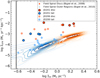 |
Fig. 7. Relation between the star formation rate density and H I surface density. The red and blue points are the main galaxy body and tail of JO201, respectively. Corresponding pixels of the JO206 are plotted in the same colour but more transparent. The pixels are plotted independently per beam to avoid showing correlated pixel values in a beam. Orange density contours are the inner regions (discs) of field spiral galaxies selected from the THINGS sample from Bigiel et al. (2008) convolved with the H I beam. Light blue density contours represent the outer regions of spiral galaxies in the field (Bigiel et al. 2010) also convolved with the H I beam. The solid vertical line indicates our general H I sensitivity limit. |
From this plot it is evident that both the disc and tail of these galaxies are forming stars at higher rate for a given H I surface density compared to THINGS galaxies. For both, JO201 and JO206, the discs show star formation rate that is about 10 times higher on average than that of normal galaxies. However, as stated in Ramatsoku et al. (2019) these are regions where the H I column density peaks at nH I > 1.2 × 10²⁰ atoms cm−2 (∼0.9 M⊙ pc−2). In the tails JO201 appears to have slightly higher star formation rate on average (3 times higher) at a given H I surface density compared to the field counterparts.
The physical reasons for the observed enhanced SFE in the disc and tail of JO201 and JO206 may be explained by combining our H I data with Fig. 7 in Moretti et al. (2018), which shows their SFR as a function of H2 from APEX data. From that plot the SFR of these galaxies appears to be low for the amount of H2 detected. In our study we find that the SFR is high for the amount of H I detected. This implies that the H2/H I ratio is high for these galaxies. A similar abundance of H2 and deficiency of H I (from upper limits) has also been reported in ESO137−001 which is another jellyfish galaxy that is not in the GASP sample (Jachym et al. 2014, 2019). The cause of this high ratio is currently not known and will be investigated in future papers. An interesting related observation is that, in a recent study of the magnetic field in one of the GASP jellyfish galaxies finds magnetic field lines and synchrotron emission in the disc and tail of JO206. It is, therefore, possible that there is some shielding of the gas by the magnetic field which prevents the gas from evaporating into the hot ICM thus continue to form stars at a high rate even in the tails.
5.4. Comparing the physical and environmental properties of JO201 and JO206
In the previous sections we discussed the H I and star formation properties of JO201 and JO206. Both galaxies show a strong displacement of the H I relative to the stellar body (on the sky and/or in velocity); they have comparable stellar masses and H I deficiencies, and they are forming stars at a similar rate, which is enhanced compared to that of galaxies with similar stellar and H I mass. The interaction with the host cluster is thus having a similar effect on JO201 and JO206. This may seem strange given that the two galaxies are nearly identical, first in-fallers in two very different clusters (Bellhouse et al. 2017, 2019; Poggianti et al. 2017a; Jaffe et al. 2018; see also Table 1). JO201 resides in a much more massive and denser cluster than JO206, and thus is expected to experience stronger ram pressure effects than the latter. In this section we attempt to understand whether the similarity between the two galaxies can at least in principle be explained despite the large difference between their host clusters.
Comparison of physical and environmental properties of JO201 and JO206.
Throughout this study we have assumed instantaneous ram pressure following the Gunn & Gott (1972) description of a homogeneous and symmetrical ICM. It is formulated as  , where vgal, is the differential velocity of the galaxy with respect to the cluster and ρICM is the ICM density, which is parametrised with a β-model, ρICM = ρ0[1 + (rgal/rc)2]−3β/2 (Cavaliere & Fusco-Femiano 1976). For this density profile ρ0 is the central density, rc is the core radius of the cluster, β is the slope parameter and rgal is the projected distance of the galaxy from the cluster centre.
Using the aforementioned descriptions and the observed (i.e. projected) rgal and vgal of JO201 and JO206, we measure Pram = 2.6 × 10⁻¹¹ Nm−2 and 4.2 × 10⁻¹³ Nm−2, respectively. These estimates confirm our earlier statement that we expect stronger ram pressure effects on JO201 than JO206, at odds with the similarities between the two galaxies. We recall, however, that JO206 is falling into IIZw108 along the plane of the sky and consequently, its observed velocity is only a lower limit on its true 3D orbital velocity (v3D) around the cluster, while the projected distance is likely close to its true 3D orbital radius (i.e.  ≈
≈  ). JO201 on the other hand is falling into A 85 along the line-of-sight such that
  ≈
≈  , while its projected distance from the cluster is a lower limit on its true 3D orbital radius.
In what follows we try to establish whether the large difference in the ram pressure estimates for JO201 and JO206 is thus a result of projection effects causing an underestimation of  and/or
  – while we assume that
  and
and  are equal to their measured, projected values.
In Fig. 8 we use a toy model to investigate what 3D velocities JO206 needs to have in IIZw108 so that it experiences the same Pram (normalised by gravitational restoring force) as JO201 as a function of 3D distances of JO201 from the centre of its host cluster A 85. We built this plot by varying ρICM with  according to the β-model of A85.
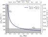 |
Fig. 8. Toy model showing what 3D velocity JO206 needs to have within the IIZw108 cluster in order to experience the same Pram as JO201 (normalised by the gravitational restoring force Πgal), as a function of 3D distance of JO201 from the centre of the A 85 cluster. The blue curve indicates equal ram pressure strengths by the ICM of the clusters hosting JO201 (A 85) and JO206 (IIZw108) relative to the galaxies’ restoring force. Hatched vertical and horizontal regions represent forbidden regions given the measured, projected cluster-centric radius and velocity of JO201 and JO206, respectively. The quantities |


We compare the ram pressure strengths with the restoring gravitational force per unit area of these galaxies defined as, ∏gal = 2πGΣgΣs, where G is the gravitational constant, Σg and Σs are the gas and stellar surface densities assuming an exponential profile of Σ = Σ0e−rt/Rd where rt is the radial distance from the galaxy centre, and Rd is the scale-length of the stellar disc. For this toy model we fix ∏gal at a radial distance of rt = 2Rd which corresponds approximately to the distance from the galaxy centre at which the stripping conditions (Pram/∏gal > 1) are met (see Poggianti et al. 2017a; Bellhouse et al. 2019).
Figure 8 shows the curve of equal ratio Pram/Πgal for a range of 3D velocities and radii for JO206 and JO201, respectively. From this plot we deduce and conclude that there is a significantly large range of reasonable values of  and
and  of JO201 and JO206 to explain the similar H I and star formation properties given the similarity of their stellar mass and morphology. We note that, assuming a Navarro et al. (1996) potential for A 85, the distance of JO201 from the cluster centre should be approximately
 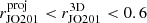 R200 ∼ 1.4 Mpc for it to remain bound to the A 85 cluster. Thus there is a region of Fig. 8 where JO201 and JO206 can experience similar ram-pressure stripping and JO201 is bound to its host cluster.
6. Summary
Within the context of the GASP survey we have examined the H I gas phase of the jellyfish galaxy, JO201. The galaxy is a member of the massive cluster A 85 with total mass of M200 ∼ 1.6 × 10¹⁵ M⊙ and a velocity dispersion, σcl ∼ 982 ± 55 km s−1 (Moretti et al. 2017). It is falling into the centre of this cluster along the line-of-sight with a velocity of = 3.4σcl, and has long Hα tails resulting from the ram pressure exerted by the cluster ICM. In this paper we studied its H I content in relation to the star formation activity, and compared it to JO206 a similar jellyfish which resides in a significantly smaller cluster. Here we summarise our findings:
-
For JO201 we measure a total H I mass of MHI = 1.65 × 10⁹ M⊙. The galaxy is H I deficient because this H I mass is ∼60% lower than expected based on its stellar mass and surface density. In Ramatsoku et al. (2019), we reported a similar H I deficiency of ∼50% for JO206.
-
The H I projected spatial distribution of JO201 is slightly perturbed but mostly close to the stellar disc. We find only a short H I tail coinciding with the clumpy 40 kpc long Hα tail. No H I is detected along the longer ∼100 kpc long diffuse Hα, although we cannot rule out the presence of dense H I clumps of similar size as the Hα clumps, whose signal would be diluted below detectability due to the large H I PSF. The close confinement of the H I to the disc is probably due to projection effect since we also find that all of the H I is strongly redshifted relative to the stars (100 km s−1 or more) and is likely already outside of the stellar body in 3D.
-
An examination of the star formation rate in relation to the H I content shows that JO201 has an enhanced SFR compared to field galaxies of the same stellar mass for its observed H I content. We find that the time it would take to deplete its H I through star formation at its current rate is ∼0.27 Gyr (similarly that of JO206 – 0.5 Gyr) which is much shorter than that of spiral galaxies in the field (∼2 Gyr; Leroy et al. 2008). Given its observed SFR, JO201 would need to have ten times its current H I mass in order to be a “normal” spiral.
-
We conducted the resolved pixel-by-pixel analysis of the H I surface density and the star formation rate density of JO201 for both the tail and disc. These properties were then compared with those of field galaxies from the THINGS. We found that similarly to JO206, the star formation efficiency of JO201 is about 10 times higher compared to that of field galaxies everywhere within the H I distribution.
Generally we observe similar physical properties for JO201 and JO206 based on their H I mass, stellar masses and star formation rates. This would mean that the galaxies are experiencing similar ram pressure effects. This finding may appear inconsistent with the different environments in which these galaxies lie. However, we showed that when projection effects are taken into account the 3D position and velocity of the two galaxies within their respective (and very different) host clusters may well result in comparable ram pressure strengths relative to their restoring forces. The similarities between JO201 and JO206 in terms of H I and SFR properties can therefore be explained despite the fact that they live in very different host clusters.
The dust correction was estimated from the Balmer decrements measured from the MUSE spectra.
Acknowledgments
We thank the anonymous referee for the useful comments and suggestions. We also wish to thank Toby Brown for his invaluable help with the scaling relations. This project has received funding from the European Research Council (ERC) under the European Union’s Horizon 2020 research and innovation programme grant agreement no. 679627 and no.833824, project name FORNAX and GASP, respectively. We acknowledge funding from the agreement ASI-INAF n.2017-14-H.0, as well as from the INAF main-stream funding programme. M. R’s research is supported by the SARAO HCD programme via the “New Scientific Frontiers with Precision Radio Interferometry” research group grant. M.R. acknowledges support from the Italian Ministry of Foreign Affairs and International Cooperation (MAECI Grant Number ZA18GR02) and the South African Department of Science and Technology’s National Research Foundation (DST-NRF Grant Number 113121) as part of the ISARP RADIOSKY2020 Joint Research Scheme. B.V. and M.G. also acknowledge the Italian PRIN-Miur 2017 (PI A. Cimatti). Y.J. acknowledges financial support from CONICYT PAI (Concurso Nacional de Insercion en la Academia 2017), No. 79170132 and FONDECYT Iniciación 2018 No. 11180558. M.V. acknowledges support by the Netherlands Foundation for Scientific Research (NWO) through VICI grant 016.130.338. This work is based on observations collected at the European Organisation for Astronomical Research in the southern hemisphere under ESO programme 196.B-0578 (PI B.M. Poggianti). This work made use of THINGS, “The H I Nearby Galaxy Survey” (Walter et al. 2008). This paper makes use of the VLA data (Project code: VLA/17A-293). The National Radio Astronomy Observatory is a facility of the National Science Foundation operated under cooperative agreement by Associated Universities, Inc. (Part of) the data published here have been reduced using the CARAcal pipeline, partially supported by BMBF project 05A17PC2 for D-MeerKAT. Information about CARAcal can be obtained online under the https://caracal.readthedocs.io/en/latest/.
References
- Abramson, A., & Kenney, J. D. P. 2014, AJ, 147, 63 [NASA ADS] [CrossRef] [Google Scholar]
- Abramson, A., Kenney, J. D. P., Crowl, H. H., et al. 2011, AJ, 141, 164 [NASA ADS] [CrossRef] [Google Scholar]
- Bellhouse, C., Jaffé, Y. L., Hau, G. K. T., et al. 2017, ApJ, 844, 49 [NASA ADS] [CrossRef] [Google Scholar]
- Bellhouse, C., Jaffé, Y. L., McGee, S. L., et al. 2019, MNRAS, 485, 1157 [CrossRef] [Google Scholar]
- Bigiel, F., Leroy, A., Walter, F., et al. 2008, AJ, 136, 2846 [NASA ADS] [CrossRef] [Google Scholar]
- Bigiel, F., Leroy, A., Walter, F., et al. 2010, AJ, 140, 1194 [NASA ADS] [CrossRef] [Google Scholar]
- Biviano, A., Moretti, A., Paccagnella, A., et al. 2017, A&A, 607, A81 [NASA ADS] [CrossRef] [EDP Sciences] [Google Scholar]
- Boissier, S., Boselli, A., Duc, P.-A., et al. 2012, A&A, 545, A142 [NASA ADS] [CrossRef] [EDP Sciences] [Google Scholar]
- Boselli, A., & Gavazzi, G. 2006, PASP, 118, 517 [NASA ADS] [CrossRef] [Google Scholar]
- Boselli, A., Gavazzi, G., Lequeux, J., et al. 1997, A&A, 327, 522 [NASA ADS] [Google Scholar]
- Boselli, A., Cuillandre, J. C., Fossati, M., et al. 2016, A&A, 587, A68 [NASA ADS] [CrossRef] [EDP Sciences] [Google Scholar]
- Bravo-Alfaro, H., Szomoru, A., Cayatte, V., Balkowski, C., & Sancisi, R. 1997, A&AS, 126, 537 [NASA ADS] [CrossRef] [EDP Sciences] [Google Scholar]
- Brown, T., Catinella, B., Cortese, L., et al. 2015, MNRAS, 452, 2479 [NASA ADS] [CrossRef] [Google Scholar]
- Catinella, B., Schiminovich, D., Kauffmann, G., et al. 2010, MNRAS, 403, 683 [NASA ADS] [CrossRef] [Google Scholar]
- Cava, A., Bettoni, D., Poggianti, B. M., et al. 2009, A&A, 495, 707 [NASA ADS] [CrossRef] [EDP Sciences] [Google Scholar]
- Cavaliere, A., & Fusco-Femiano, R. 1976, A&A, 500, 95 [NASA ADS] [Google Scholar]
- Chabrier, G. 2003, PASP, 115, 763 [Google Scholar]
- Chung, A., van Gorkom, J. H., Kenney, J. D. P., Crowl, H., & Vollmer, B. 2009, AJ, 138, 1741 [NASA ADS] [CrossRef] [Google Scholar]
- Cortese, L., Gavazzi, G., Boselli, A., et al. 2006, A&A, 453, 847 [Google Scholar]
- Cortese, L., Marcillac, D., Richard, J., et al. 2007, MNRAS, 376, 157 [NASA ADS] [CrossRef] [Google Scholar]
- Cowie, L. L., & Songaila, A. 1977, Nature, 266, 501 [Google Scholar]
- Cramer, W. J., Kenney, J. D. P., Sun, M., et al. 2019, ApJ, 870, 63 [Google Scholar]
- Deb, T., Verheijen, M. A. W., Gullieuszik, M., et al. 2020, MNRAS, 494, 5029 [Google Scholar]
- Di Teodoro, E. M., & Fraternali, F. 2015, MNRAS, 451, 3021 [Google Scholar]
- Doyle, M. T., & Drinkwater, M. J. 2006, MNRAS, 372, 977 [Google Scholar]
- Ebeling, H., Stephenson, L. N., & Edge, A. C. 2014, ApJ, 781, L40 [Google Scholar]
- Fasano, G., Marmo, C., Varela, J., et al. 2006, A&A, 445, 805 [NASA ADS] [CrossRef] [EDP Sciences] [Google Scholar]
- Fasano, G., Vanzella, E., Dressler, A., et al. 2012, MNRAS, 420, 926 [Google Scholar]
- Fossati, M., Fumagalli, M., Boselli, A., et al. 2016, MNRAS, 455, 2028 [Google Scholar]
- Fumagalli, M., Fossati, M., Hau, G. K. T., et al. 2014, MNRAS, 445, 4335 [Google Scholar]
- Gavazzi, G., Giovanelli, R., Haynes, M. P., et al. 2008, A&A, 482, 43 [NASA ADS] [CrossRef] [EDP Sciences] [Google Scholar]
- Gavazzi, G., Consolandi, G., Gutierrez, M. L., Boselli, A., & Yoshida, M. 2018, A&A, 618, A130 [NASA ADS] [CrossRef] [EDP Sciences] [Google Scholar]
- George, K., Poggianti, B. M., Gullieuszik, M., et al. 2018, MNRAS, 479, 4126 [Google Scholar]
- Gullieuszik, M., Poggianti, B., Fasano, G., et al. 2015, A&A, 581, A41 [NASA ADS] [CrossRef] [EDP Sciences] [Google Scholar]
- Gunn, J. E., & Gott, J. R., III 1972, ApJ, 176, 1 [Google Scholar]
- Haynes, M. P., Giovanelli, R., & Chincarini, G. L. 1984, ARA&A, 22, 445 [Google Scholar]
- Hester, J. A., Seibert, M., Neill, J. D., et al. 2010, ApJ, 716, L14 [Google Scholar]
- Huang, S., Haynes, M. P., Giovanelli, R., & Brinchmann, J. 2012, ApJ, 756, 113 [Google Scholar]
- Jachym, P., Combes, F., Cortese, L., Sun, M., & Kenney, J. D. P. 2014, ApJ, 792, 11 [Google Scholar]
- Jáchym, P., Kenney, J. D. P., Sun, M., et al. 2019, ApJ, 883, 145 [Google Scholar]
- Jaffé, Y. L., Smith, R., Candlish, G. N., et al. 2015, MNRAS, 448, 1715 [Google Scholar]
- Jaffe, Y. L., Poggianti, B. M., Moretti, A., et al. 2018, MNRAS, 476, 4753 [Google Scholar]
- Kapferer, W., Sluka, C., Schindler, S., Ferrari, C., & Ziegler, B. 2009, A&A, 499, 87 [NASA ADS] [CrossRef] [EDP Sciences] [Google Scholar]
- Kenney, J. D. P., Tal, T., Crowl, H. H., Feldmeier, J., & Jacoby, G. H. 2008, ApJ, 687, L69 [Google Scholar]
- Leroy, A. K., Walter, F., Brinks, E., et al. 2008, AJ, 136, 2782 [Google Scholar]
- Martinsson, T. P. K., Verheijen, M. A. W., Bershady, M. A., et al. 2016, A&A, 585, A99 [NASA ADS] [CrossRef] [EDP Sciences] [Google Scholar]
- McPartland, C., Ebeling, H., Roediger, E., & Blumenthal, K. 2016, MNRAS, 455, 2994 [NASA ADS] [CrossRef] [Google Scholar]
- Moretti, A., Gullieuszik, M., Poggianti, B., et al. 2017, A&A, 599, A81 [NASA ADS] [CrossRef] [EDP Sciences] [Google Scholar]
- Moretti, A., Paladino, R., Poggianti, B. M., et al. 2018, MNRAS, 480, 2508 [Google Scholar]
- Navarro, J. F., Frenk, C. S., & White, S. D. M. 1996, ApJ, 462, 563 [NASA ADS] [CrossRef] [Google Scholar]
- Nulsen, P. E. J. 1982, MNRAS, 198, 1007 [Google Scholar]
- Owen, F. N., Keel, W. C., Wang, Q. D., Ledlow, M. J., & Morrison, G. E. 2006, AJ, 131, 1974 [Google Scholar]
- Owers, M. S., Couch, W. J., Nulsen, P. E. J., & Randall, S. W. 2012, ApJ, 750, L23 [Google Scholar]
- Perley, R., Napier, P., Jackson, J., et al. 2009, IEEE Proc., 97, 1448 [Google Scholar]
- Poggianti, B. M., Fasano, G., Omizzolo, A., et al. 2016, AJ, 151, 78 [Google Scholar]
- Poggianti, B. M., Moretti, A., Gullieuszik, M., et al. 2017a, ApJ, 844, 48 [Google Scholar]
- Poggianti, B. M., Jaffé, Y. L., Moretti, A., et al. 2017b, Nature, 548, 304 [Google Scholar]
- Poggianti, B. M., Gullieuszik, M., Tonnesen, S., et al. 2019, MNRAS, 482, 4466 [Google Scholar]
- Quilis, V., Moore, B., & Bower, R. 2000, Science, 288, 1617 [Google Scholar]
- Radovich, M., Poggianti, B., Jaffé, Y. L., et al. 2019, MNRAS, 486, 486 [Google Scholar]
- Ramatsoku, M., Serra, P., Poggianti, B. M., et al. 2019, MNRAS, 487, 4580 [Google Scholar]
- Saintonge, A., Catinella, B., Cortese, L., et al. 2016, MNRAS, 462, 1749 [Google Scholar]
- Scott, T. C., Bravo-Alfaro, H., Brinks, E., et al. 2010, MNRAS, 403, 1175 [Google Scholar]
- Serra, P., Westmeier, T., Giese, N., et al. 2015, MNRAS, 448, 1922 [Google Scholar]
- Smith, R. J., Lucey, J. R., Hammer, D., et al. 2010, MNRAS, 408, 1417 [Google Scholar]
- Steinhauser, D., Schindler, S., & Springel, V. 2016, A&A, 591, A51 [NASA ADS] [CrossRef] [EDP Sciences] [Google Scholar]
- Sun, M., Donahue, M., & Voit, G. M. 2007, ApJ, 671, 190 [Google Scholar]
- Varela, J., D’Onofrio, M., Marmo, C., et al. 2009, A&A, 497, 667 [NASA ADS] [CrossRef] [EDP Sciences] [Google Scholar]
- Venkatapathy, Y., Bravo-Alfaro, H., Mayya, Y. D., et al. 2017, AJ, 154, 227 [Google Scholar]
- Verdugo, C., Combes, F., Dasyra, K., Salomé, P., & Braine, J. 2015, A&A, 582, A6 [NASA ADS] [CrossRef] [EDP Sciences] [Google Scholar]
- Vollmer, B., Cayatte, V., van Driel, W., et al. 2001, A&A, 369, 432 [NASA ADS] [CrossRef] [EDP Sciences] [Google Scholar]
- Vollmer, B., Wong, O. I., Braine, J., Chung, A., & Kenney, J. D. P. 2012, A&A, 543, A33 [NASA ADS] [CrossRef] [EDP Sciences] [Google Scholar]
- Vulcani, B., Poggianti, B. M., Gullieuszik, M., et al. 2018, ApJ, 866, L25 [Google Scholar]
- Walter, F., Brinks, E., de Blok, W. J. G., et al. 2008, AJ, 136, 2563 [Google Scholar]
- Wang, J., Koribalski, B. S., Serra, P., et al. 2016, MNRAS, 460, 2143 [Google Scholar]
- Yagi, M., Yoshida, M., Komiyama, Y., et al. 2010, AJ, 140, 1814 [Google Scholar]
- Yoon, H., Chung, A., Smith, R., & Jaffé, Y. L. 2017, ApJ, 838, 81 [Google Scholar]
- Yoshida, M., Yagi, M., Komiyama, Y., et al. 2008, ApJ, 688, 918 [Google Scholar]
All Tables
All Figures
|
Fig. 1. A multiwavelength composite image illustrating all the data available for JO201. The NUV data is shown in violet overlaid on an optical V-band image in grayscale from WINGS. In red we overlay the Hα emission from MUSE. The 12CO(2–1) observations are illustrated by the approximate FWHM of the APEX beam. |
| In the text | |
|
Fig. 2. Left panel: VLA H I column density contours overlaid on the V-band image of JO201 from WINGS. Contour levels are drawn at column densities of 4, 8, 12, ... × 1019 atoms cm−2. The FWHM beam size of 16″ × 25″ is indicated by the blue ellipse. The red contours represent the stellar disc and the black contour is the H I disc (see text for a definition). Right panel: Hα emission with H I column density contours (same levels as the left panel) overlaid. The red opaque patch is the stellar disc and the black contour is the H I disc. The black circle is the region over which we estimate the H I flux density as described in the text. |
| In the text | |
|
Fig. 3. Position velocity diagrams (PVDs) extracted from the H I cube along the three 1.25′ wide right ascension slices indicated in the top right corner. The Hα emission convolved with the H I PSF is shown in orange. For reference, the red contour in the middle panel represents the stellar velocities extracted from Bellhouse et al. (2017) (no convolution to the HI angular resolution was performed). The Hα contours are drawn at surface brightness levels of 1 × 10n erg s−1 cm2 where n = −10, −9, −8 ⋯. The blue contours are the H I emission from the cube drawn at flux densities of 0.3, 0.4, 0.5 ... mJy beam−1 and the negative H I contours are drawn at −0.3, −0.2 ... mJy beam−1. The vertical dashed line is the systemic velocity of the galaxy and the horizontal line is the optical centre. Velocities in the PVDs are in the optical definition using the barycentric standard-of-rest. |
| In the text | |
|
Fig. 4. Star formation rate density map (Bellhouse et al. 2019) with H I emission contours overlaid. The contours are at H I column density levels of 4, 8, 12, ... × 1019 atoms cm−2. The FWHM beam size of 25″ × 16″ is shown by the blue ellipse. |
| In the text | |
|
Fig. 5. Average stacked H I fraction as function of the stellar mass (Brown et al. 2015). The relation is separated into galaxies with stellar surface brightness comparable to that of JO201 and JO206 within a factor of 4. The scatter in the mass bins is illustrate by the error bars. JO201 is represented by the green asterisk and JO206 by the blue asterisk. |
| In the text | |
|
Fig. 6. H I−SFR scaling relation showing the star formation rate vs H I mass for galaxies with the same stellar masses as JO201 and JO206. Grey hexagons are galaxies from the control sample (GASS) and the green and blue asterisk represent the JO201 and JO206 galaxies, respectively. The dotted lines indicate the fixed H I depletion times in yr. |
| In the text | |
|
Fig. 7. Relation between the star formation rate density and H I surface density. The red and blue points are the main galaxy body and tail of JO201, respectively. Corresponding pixels of the JO206 are plotted in the same colour but more transparent. The pixels are plotted independently per beam to avoid showing correlated pixel values in a beam. Orange density contours are the inner regions (discs) of field spiral galaxies selected from the THINGS sample from Bigiel et al. (2008) convolved with the H I beam. Light blue density contours represent the outer regions of spiral galaxies in the field (Bigiel et al. 2010) also convolved with the H I beam. The solid vertical line indicates our general H I sensitivity limit. |
| In the text | |
|
Fig. 8. Toy model showing what 3D velocity JO206 needs to have within the IIZw108 cluster in order to experience the same Pram as JO201 (normalised by the gravitational restoring force Πgal), as a function of 3D distance of JO201 from the centre of the A 85 cluster. The blue curve indicates equal ram pressure strengths by the ICM of the clusters hosting JO201 (A 85) and JO206 (IIZw108) relative to the galaxies’ restoring force. Hatched vertical and horizontal regions represent forbidden regions given the measured, projected cluster-centric radius and velocity of JO201 and JO206, respectively. The quantities |
| In the text | |
Current usage metrics show cumulative count of Article Views (full-text article views including HTML views, PDF and ePub downloads, according to the available data) and Abstracts Views on Vision4Press platform.
Data correspond to usage on the plateform after 2015. The current usage metrics is available 48-96 hours after online publication and is updated daily on week days.
Initial download of the metrics may take a while.