| Issue |
A&A
Volume 638, June 2020
|
|
|---|---|---|
| Article Number | A62 | |
| Number of page(s) | 12 | |
| Section | The Sun and the Heliosphere | |
| DOI | https://doi.org/10.1051/0004-6361/202037810 | |
| Published online | 11 June 2020 | |
Transient brightenings in the quiet Sun detected by ALMA at 3 mm
1
Physics Department, University of Ioannina, Ioannina 45110, Greece
e-mail: anindos@uoi.gr
2
National Radio Astronomy Observatory, 520 Edgemont Road, Charlottesville, VA 22903, USA
Received:
24
February
2020
Accepted:
8
April
2020
Aims. We investigate transient brightenings, that is, weak, small-scale episodes of energy release, in the quiet solar chromosphere; these episodes can provide insights into the heating mechanism of the outer layers of the solar atmosphere.
Methods. Using Atacama Large Millimeter/submillimeter Array (ALMA) observations, we performed the first systematic survey for quiet Sun transient brightenings at 3 mm. Our dataset included images of six 87″ × 87″ fields of view of the quiet Sun obtained with angular resolution of a few arcsec at a cadence of 2 s. The transient brightenings were detected as weak enhancements above the average intensity after we removed the effect of the p-mode oscillations. A similar analysis, over the same fields of view, was performed for simultaneous 304 and 1600 Å data obtained with the Atmospheric Imaging Assembly.
Results. We detected 184 3 mm transient brightening events with brightness temperatures from 70 K to more than 500 K above backgrounds of ∼7200 − 7450 K. All events showed light curves with a gradual rise and fall, strongly suggesting a thermal origin. Their mean duration and maximum area were 51.1 s and 12.3 Mm2, respectively, with a weak preference of appearing at network boundaries rather than in cell interiors. Both parameters exhibited power-law behavior with indices of 2.35 and 2.71, respectively. Only a small fraction of ALMA events had either 304 or 1600 Å counterparts but the properties of these events were not significantly different from those of the general population except that they lacked their low-end energy values. The total thermal energies of the ALMA transient brightenings were between 1.5 × 1024 and 9.9 × 1025 erg and their frequency distribution versus energy was a power law with an index of 1.67 ± 0.05. We found that the power per unit area provided by the ALMA events could account for only 1% of the chromospheric radiative losses (10% of the coronal ones).
Conclusions. We were able to detect, for the first time, a significant number of weak 3 mm quiet Sun transient brightenings. However, their energy budget falls short of meeting the requirements for the heating of the upper layers of the solar atmosphere and this conclusion does not change even if we use the least restrictive criteria possible for the detection of transient brightenings.
Key words: Sun: radio radiation / Sun: chromosphere / Sun: atmosphere
© ESO 2020
1. Introduction
Episodes of energy release are ubiquitous in the solar atmosphere and may occur in active regions, the boundaries of the quiet Sun network cells, and even in the cell interior and coronal holes. The larger events, called flares, occur almost exclusively in active regions. Small-scale events occur everywhere and all the time, both in active regions and the quiet Sun, and the detection limit of these events is determined by the sensitivity as well as the spatial, temporal, and spectral resolution of the instrument. Therefore it is not a surprise that every time a new instrument with improved specifications appears, new varieties of such events, sometimes differently termed, are reported.
There is substantial literature on the detection of weak transient activity starting from early Yohkoh soft X-ray (e.g., Shimizu 1995) and Extreme ultraviolet Imaging Telescope (EIT) extreme ultraviolet (EUV) observations (e.g., Benz & Krucker 1998; Krucker & Benz 1998; Berghmans et al. 1998) to observations from the Transition Region and Coronal Explorer (TRACE; e.g., Aschwanden et al. 2000; Parnell & Jupp 2000), Ramaty High Energy Solar Spectroscopic Imager (RHESSI; e.g., Hannah et al. 2008), Hinode’s X-Ray Telescope (XRT) and EUV Imaging Spectrometer (EIS; see Hinode Review Team 2019, and references therein); Atmospheric Imaging Assembly (AIA; e.g., Joulin et al. 2016; Ulyanov et al. 2019), Interface Region Imaging Spectrograph (IRIS; e.g., Peter et al. 2014; Vissers et al. 2015; Rouppe van der Voort et al. 2016), Focusing Optics X-ray Solar Imager (FOXSI), and the Nuclear Spectroscopic Telescope Array (NuSTAR; Marsh et al. 2018). Monte Carlo simulations of the statistical signatures of very weak events were presented by Dillon et al. (2019).
Radio observations have also been used for the detection of weak transient activity. The great sensitivity of the radio range to small nonthermal electron populations that are expected as a by-product of the reconnection process have allowed radio observations to reveal the occurrence not only of thermal events (e.g., White et al. 1995) but also of nonthermal events whose emission has been attributed either to the gyrosynchrotron mechanism (e.g., Krucker et al. 1997; Gary et al. 1997; Nindos et al. 1999) or to the plasma emission mechanism (e.g., Ramesh et al. 2010; Saint-Hilaire et al. 2013; Suresh et al. 2017).
Weak transient activity can be detected either indirectly or directly. Indirect detections include evidence about the occurrence of unresolved events by analyzing asymmetries of X-ray intensity fluctuations (e.g., Katsukawa & Tsuneta 2001; Terzo et al. 2011), time lags of EUV light curves of coronal loops (e.g., Viall & Klimchuk 2012), and possibly subtle enhancements in the blue wing of hot spectral lines (e.g., Hara et al. 2008; De Pontieu et al. 2009; Brooks & Warren 2012). Direct evidence includes the detection of time variability of the intensity (e.g., Berghmans et al. 1998) or the emission measure (e.g., Krucker & Benz 1998) of clusters of pixels above some predefined threshold. In most studies, most of the detected events are spatially unresolved (e.g., Benz & Krucker 1999), but some events may exhibit a loop-like morphology (e.g., White et al. 1995; Benz & Krucker 1998; Warren et al. 2007), a jet-like morphology (e.g., Tian et al. 2014; Alissandrakis et al. 2015), show evidence of two-loop interactions (e.g., Shimizu et al. 1994; Alissandrakis et al. 2017a), or even resemble Ellerman bombs (e.g., Shetye et al. 2018).
Several authors have studied the contribution of weak transient events to the heating of the upper atmosphere. These studies are motivated by the nanoflare heating conjecture first proposed by Parker (1988). Nanoflares, events with energies less than 1024 erg, are expected to occur as a result of magnetic reconnection in elemental, tangled magnetic flux tubes that are below the resolution limit of present-day instruments. So far only detections of individual events with energy down to the “high-end” limit of Parker’s estimate have been achieved (e.g., Berghmans et al. 1998; Parnell & Jupp 2000; Aschwanden et al. 2000; Winebarger et al. 2013; Régnier et al. 2014; Joulin et al. 2016; Subramanian et al. 2018). It has been argued that these small events could heat the upper atmosphere if the energy released during various types of flare-like activity follows a power-law frequency distribution with energy that has an index α ≥ 2 (e.g., Hudson 1991). Several authors have presented such computations (e.g., Crosby et al. 1993; Shimizu 1995; Krucker & Benz 1998; Aschwanden et al. 2000; Benz & Krucker 2002). Most studies (with some notable exceptions, e.g., Krucker & Benz 1998; Parnell & Jupp 2000; Benz & Krucker 2002) show that the above requirement is not satisfied.
Any attempt to solve the coronal heating problem cannot circumvent the problem of determining the mechanisms by which chromospheric plasma is heated and lifted to form the corona. The detection of ubiquitous weak enhancements in the blue wing of hot spectral lines has been interpreted by some authors (e.g., De Pontieu et al. 2009) as evidence of upflows associated with chromospheric spicules that provide a significant mass supply mechanism for the corona. This scenario, which ultimately places the source of coronal heating in the chromosphere, has been contested by Klimchuk (2012) who argued that the preheated plasma provided by spicules is not sufficient to fill the corona, but even if it is, this would require additional heating to remain hot as it rises into the corona.
No matter what the role of chromospheric spicules in coronal heating is, the energy requirements to heat the quiet chromosphere is about one order of magnitude higher than those for the quiet corona (Withbroe & Noyes 1977). Then an obvious question is to what extent chromospheric small-scale energy release events contribute to the heating of the chromosphere in general, and the quiet chromosphere in particular. The calculation of the physical parameters of such events in optical and UV observations is complicated because this calculation relies on complex physical effects such as partial and time-dependent ionization and departures from local thermodynamic equilibrium (e.g., Leenaarts et al. 2013). However, that task can be facilitated by using millimeter wavelength observations of the quiet chromosphere because the relevant emission mechanism is thermal free-free, which does not suffer from the problems mentioned above and because, thanks to the Rayleigh-Jeans law, the recorded brightness temperature is linearly linked to the electron temperature (e.g., Shibasaki et al. 2011; Wedemeyer et al. 2016; but see Martinez-Sykora et al. 2020 who suggest that the interpretation of millimeter-λ continua might be more complicated than these simple expectations).
The availability of millimeter-λ solar observations with Atacama Large Millimeter/submillimeter Array (ALMA) has the potential to provide new insights into the physics of the chromosphere thanks to the superior spatial and temporal resolution and sensitivity of the instrument. Observations of the quiet Sun with ALMA have been reported by Shimojo et al. (2017a,b), White et al. (2017), Alissandrakis et al. (2017b), Bastian et al. (2017), Yokoyama et al. (2018), Nindos et al. (2018), Loukitcheva et al. (2019), Brajša et al. (2018), Jafarzadeh et al. (2019), Selhorst et al. (2019), Molnar et al. (2019), Patsourakos et al. (2020), and Wedemeyer et al. (2020). Among those articles, detection of single weak transient events was reported by Shimojo et al. (2017b), who studied a plasmoid ejection associated with an X-ray bright point, and by Yokoyama et al. (2018) who reported jet-like activity at 3 mm.
In this article we present the first systematic survey for weak small-scale energy release events in the quiet Sun using ALMA data obtained at 3 mm. Different authors use different terminology for such events; in what follows we adopt the term “transient brightenings”. Our article is structured as follows: In Sect. 2 we discuss the observations and our analysis. The statistics and properties of the detected transient brightenings are given in Sect. 3 while their implications for chromospheric heating are discussed in Sect. 4. Finally, we present conclusions in Sect. 5.
2. Observations and data analysis
We used the ALMA observations of the quiet Sun presented by Nindos et al. (2018), which included seven 120″ circular fields of view (targets), observed at 100 GHz (3 mm) on March 16, 2017. These targets, numbered from 1 to 7, correspond to μ = [0.16, 0.34, 0.52, 0.72, 0.82, 0.92, 1.00] along a position angle of 135° from the center-North direction and thus supplied a center-to-limb coverage (μ = cos θ, where θ is the angle between the line of sight and the local vertical). For our analysis we used only targets 2–7 because a significant part of the target 1 field of view contained off-limb locations. Each target was observed for 10 min with a cadence of 2 s. The reduction of the ALMA data has been described by Nindos et al. (2018). The final images had pixel size of 1″ and their spatial resolution deduced from the clean beam size was about 2.5″ × 4.5″ with the exception of target 7 whose resolution was 2.3″ × 8.1″.
In our analysis we used the central 87″ × 87″ region of each field of view to avoid artifacts introduced by the primary beam correction toward the edge of the images. Since the characteristic scale of the chromospheric network is about 20″–30″, the regions we selected contain an adequate number of supergranules to allow us to perform meaningful statistics of the occurrence of 3 mm transient brightenings in the quiet Sun.
We also analyzed AIA images (same time intervals and fields of view as the ALMA images) obtained at 304 Å and 1600 Å, primarily to compare these with the 3 mm results. The cadence of the AIA images was 12 s in 304 Å and 24 s in 1600 Å. The analysis of the AIA data involved the correction for differential rotation, their convolution with the appropriate ALMA beam, and their co-alignment with the ALMA images by cross-correlating the time average images for each target. We note that the AIA 304 Å channel records primarily emission from the upper chromosphere, while the emission in 1600 Å partly comes from the upper photosphere.
For the detection of transient brightenings we used the following method. For each target we computed the light curve of each pixel. Each light curve was detrended by subtracting the running average of the time profile of a macropixel with size equal to the ALMA beam, which was centered around the pixel under consideration. The running average was computed with a kernel of 10 min (i.e., the width of the kernel was equal to the duration of observations of each target). Detrending the light curves was necessary in order to remove long-term, slowly varying trends from the data, which corresponded to neither oscillations nor transient brightening activity. The use of macropixels for the background subtraction was deemed necessary for the suppression of artifacts that may appear when a single pixel is used for the background calculation (see Berghmans et al. 1998).
Then an attempt was made to remove the effect of oscillations from the data since it is well known that p-mode oscillations are ubiquitous in ∼3 mm quiet Sun data (see White et al. 2006). Recently, Patsourakos et al. (2020) analyzed such oscillations using the same dataset as ours and found that the frequency of oscillations was 4.2 ± 1.7 mHz with an rms of about 55–75 K (i.e., approximately up to 1% of the recorded averaged brightness temperatures), while their amplitude in individual pixels can reach values as high as 350 K.
In our detrended light curves we applied a least-squares curve fitting procedure (see Roerink et al. 2000) based on the harmonic components that correspond to the oscillations detected by Patsourakos et al. (2020). The amplitude and phase of these functions were determined iteratively by removing data points with large deviations from the fitting curve. The remaining points were used for the recalculation of the coefficients until an acceptable maximum error (≲5 K) is reached or their number becomes less than five. The final sinusoidal curves were subtracted from the detrended light curves. Two examples of light curves of individual pixels appear in Fig. 1; panels a and b show the original light curves while panels d and e shows the light curves after the application of the processing described above.
 |
Fig. 1. Top row: light curves of a target 3 single pixel showing transient brightening before (a) and after (d) the processing described in Sect. 2. In this and subsequent light-curve displays, the arrows indicate the times in which the intensity exceeds the 2.5σ threshold above average. Middle row: same as top row for a pixel that did not show transient brightening. The curve in panel b has been displaced by −300 K. Bottom row: panel c shows the power spectra deduced from light curves (a) and (b), while panel f shows the power spectra deduced from light curves (d) and (e). |
The bottom row of Fig. 1 shows the power spectra deduced from the light curves presented in the same figure. Prior to the calculation of the power spectra of panel c the light curves were detrended while the light curves of panels d and e were submitted to power spectral analysis without any additional processing. Panel c shows that the p-mode oscillations stand out prominently in the power spectra resulted from the uncorrected light curves while panel f indicates that our algorithm can significantly suppress the power of p-mode oscillations (by factors of 12–17). We note that such behavior was typical for all pixels. The maximum residual p-mode power is about 30 K2 Hz−1 in the examples of Fig. 1 and can reach values as high as 40 K2 Hz−1 with a slight increase toward the limb. That trend could affect the detection of very weak events, and we return to that point in Sect. 3.
In the corrected light curves, an “event” was identified if: (i) the intensity of at least four consecutive points of the light curve was above some user-defined threshold above the average intensity of the curve, (ii) such behavior was also exhibited by a user-defined number of clusters of pixels adjacent to the pixel under consideration, and (iii) a synchrony tolerance of ±2 min between light curve peaks of the selected adjacent pixels was satisfied (see Benz & Krucker 2002 and references therein). These criteria were implemented to avoid the accidental inclusion of exceptionally large statistical fluctuations or sidelobes.
Our choices certainly affect the statistics of the detected events and this point is discussed in Sect. 3. Most of the subsequent results have been derived using a multiplication factor of 2.5σ above average intensity for the light curves (that is a threshold that has been employed in several previous studies, e.g., Berghmans et al. 1998) and a beam-size cluster of adjacent pixels for the spatial criterion (i.e., 12 pixels for targets 2–6 and 19 pixels for target 7). The latter selection is justified by the fact that due to the limited spatial resolution, the intensity of individual pixels should be correlated on the scale of the synthesized beam. In Fig. 1 the top row of light curves belong to a pixel that was part of one of the events selected by our method and the arrows point to intensities which exceed the 2.5σ threshold. On the other hand, the middle row of light curves belong to a pixel that did not show transient activity.
We followed the same procedure for the identification of transient brightenings in the AIA (see Lemen et al. 2012) 304 Å and 1600 Å data with the exception that we required one light curve point above the 2.5σ threshold instead of four consecutive points due to the lower cadence of the AIA data.
3. Statistics and properties of transient brightenings
In Fig. 2 we show how the change of our detection thresholds affects the statistics of transient brightenings in target 5. Similar results were obtained for the other targets. In the top panel we show the influence of the change of the detection threshold above background in the light curves of individual pixels that resulted from the application of our method without imposing any additional spatial coherence detection criterion. Practically all pixels show intensity variations within the 1.0–1.2σ level and this reflects the presence of noise and/or the influence of oscillations that cannot be removed completely from the light curves (see also the discussion about Fig. 1). The percentage of selected pixels drops quickly for thresholds higher than 1.7σ, exhibits an inflection point around 2.6σ, and approaches zero for thresholds higher than 3.0σ.
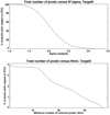 |
Fig. 2. Top: ratio of the target 5 “event pixels” with respect to the number of pixels of the whole field of view (expressed in percentage) as a function of the σ multiplication factor that determines the threshold for the detection of transient brightenings. No additional spatial coherence detection criteria have been applied for the production of these results. Bottom: same quantity as top curve but now computed as a function of the minimum number of adjacent pixels on top of the 2.5σ multiplication factor. |
In the bottom panel of Fig. 2 we show how the transient brightenings statistics are affected when we vary the event “spatial coherence” criterion (i.e., the minimum number of adjacent pixels, Nmin) on top of the 2.5σ multiplication factor. In the two plots of Fig. 2 the percentages are different; in the top panel the value that corresponds to 2.5σ is ∼10%, while in the bottom panel all values are less than 4%. This difference in the percentages is because an additional spatial coherence criterion (Nmin coherent pixels) was imposed on top of the 2.5σ threshold for the bottom curve. The number of selected event pixels shows a plateau for Nmin ≤ 12, which is the number of pixels that correspond to the beam size for targets 2–6. The plateau appears to result from the limited spatial resolution of the images, which yields the correlation of signals from individual point sources on map patches containing 12 pixels (or 19 pixels for target 7). Furthermore, the lack of appreciable changes for Nmin ≤ 12 justifies our selection of using Nmin = 12 in the subsequent analysis. The percentage of selected event pixels drops rather smoothly for Nmin > 12; the half maximum value is reached for Nmin = 23 while there is no event with more than 37 pixels.
The number of ALMA events per target that were detected after we applied our method with the 2.5σ criterion for the light curves and the beam-size patch of adjacent pixels for the spatial criterion are given in the third column of Table 1. For each target, we also give the percentages of event pixels with respect to the pixels of the whole field of view.
Statistics of transient brightenings.
In Fig. 3 we present (for all targets) histograms of the maximum brightness temperature above the background of the pixels that exhibited transient brightenings. All histograms show a rise part that is steeper than their decay part, which probably indicates that the populations of events with relatively high intensities are larger than the populations of smaller events. Equivalently, this conclusion indicates departure from Gaussianity for the maximum brightness temperature distributions, which is further supported by the analysis that is presented in this section as well as in Sect. 4. We also note that the histograms of targets 3, 5, and 6 appear bimodal, which could suggest the existence of two populations of event pixels regarding their maximum brightness temperature. The histogram widths for targets 2–6, measured at half maximum, are between 110 K and 230 K. The histogram width for target 7 is about 60 K, much more narrow than the others, and that is probably a spatial resolution effect (see Sect. 2 and Nindos et al. 2018).
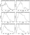 |
Fig. 3. Histograms of maximum brightness temperature above the background of the selected event pixels for all targets. |
The histograms of Fig. 3 provide hints for center-to-limb variation of the average maximum brightness temperature, Tb, max, which appears to slightly increase toward the limb. This effect is better represented in Fig. 4a, in which we plot that quantity as a function of μ. The scatter that appears in this figure is significant, however it is possible to obtain a linear least-squares fit of the data within the error bars. The center-to-limb variation of Tb, max is consistent with the slight increase of residual oscillation power toward the limb indicated by Fig. 4b: for an event detection, Tb, max needs to increase to compensate for the increase of the residual oscillatory power. Again the scatter of data points in Fig. 4b is significant but the limbward increase of residual power can easily be identified as evidenced by the least-squares fit to the data points. It is possible that the tendency reflected in Fig. 4b is due to the moderate increase of the 3 mm p-mode oscillations toward the limb (see Patsourakos et al. 2020).
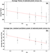 |
Fig. 4. Top: average maximum brightness temperature of the selected event pixels in each target as a function of μ. The error bars denote the standard deviation of the corresponding distributions. The red line shows the linear-squares fit to the measurements. Bottom: same as top, but for the average maximum residual oscillation power. |
There is an increase in the number of detected events toward disk center in targets 2–5 (see third column of Table 1). This trend is not shared by the number of events detected in targets 6 and (especially) 7 possibly owing to inferior seeing conditions during the observations and larger beam size (target 7). With other conditions (e.g., seeing and spatial resolution) remaining the same, we would expect fewer detections as μ decreases owing to the increased degree of obscuration due to spicules, and this is the case for targets 2–5.
A complementary approach to studying the distribution of the transient brightenings occurrence rate as a function of height in more detail could be provided by the analysis of snapshot maps made in different spectral windows (spws): for example, spw 0 (93 GHz) versus spw 3 (107 GHz). Such approach was followed by Rodger et al. (2019) for the analysis of a plasmoid ejection. However, in our analysis we summed over all spectral windows when producing the snapshot maps and therefore the results from such computations could be addressed in a future work.
For both AIA 304 Å and 1600 Å datasets we detected transient brightenings as described in Sect. 2. The number of AIA events per target, together with the percentages of event pixels with respect to each field of view, are given in the fourth (304 Å) and fifth (1600 Å) columns of Table 1. The total number of ALMA events (184) is almost equal to the total numbers of 304 Å events (199), but it is a factor of 3.4 smaller than that of the 1600 Å events.
An interesting question is how the ALMA transient brightenings correlate with the AIA brightenings. In order to find possible counterparts of the ALMA events among those detected in the AIA datasets (either 304 or 1600 Å) we requested that the two events (ALMA and AIA) have at least one common pixel and that their light curves show maxima within 15 s. We note that the cadences of the 3 mm, 304 Å, and 1600 Å data were 2, 12, and 24 s, respectively. The synchrony tolerance that we adopted was about 23–29% of the full width at half maximum (FWHM) of the average duration of the ALMA and AIA events (see Table 2). The number of paired ALMA-304 Å events and ALMA-1600 Å events appear in Cols. 6 and 7 of Table 1. Their number is much smaller than the number of the events detected independently in each database; the percentage of their pixels with respect to each field of view have not been included in Table 1 because they are all below 0.5%. We also note that we found no event appearing in all three datasets. If we increase the accepted temporal difference between maxima of the ALMA and AIA events to the average of the FWHM values of Table 2, the number of paired events roughly doubles.
Duration, size, and location of transient brightenings.
We also estimated how many ALMA transient brightenings with AIA counterparts would be expected if there was no correlation between ALMA and AIA events, and any concurrence would be by pure chance. To this end, for each target we used the percentages of the field of view occupied by the events (see the values in parentheses in Cols. 3–5 of Table 1) to find the number of pixels that could be part of paired events by pure chance. The result was divided by the mean number of pixels of the ALMA events of a given target. The number of chance concurrences ranged from less than 1 to 3 events and was always smaller than the number of detected paired events with the exceptions of target 4 and 5 ALMA-1600 Å paired events.
In Fig. 5 the pixels that participate in the events detected in target 4 are indicated with different colors. A similar picture holds for the other targets as well. The top row of the figure shows the events detected independently at a given database, while in the bottom row only the pairs of ALMA-304 Å events and ALMA-1600 Å events are indicated. In all three datasets the detected events show remarkable spatial coherence in the sense that they appear as irregularly shaped blobs.
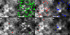 |
Fig. 5. Display of the selected pixels that correspond to transient brightenings in 1600 Å (green), 3 mm (red), and 304 Å (blue) target 4 data. Top row: all events detected at a given wavelength are denoted. Bottom row: panels e and f show only the events that appear both at 3 mm and 1600 Å, respectively, while panels g and h show only the events that appear both at 3 mm and 304 Å, respectively. In each panel the relevant average image is shown as background. |
In each snapshot image, we were able to segregate the network from the intra-network pixels using the method described by Nindos et al. (2018); that is, fit the image intensities with a second-degree polynomial and assume that the values above the fit correspond to the network. We found that the ALMA and 304 Å events show a weak tendency (∼68 − 69%) of appearing at network boundaries rather than in cell interiors (see Table 2), which confirms the visual impression from Fig. 5. The situation is somehow different at 1600 Å, where a larger portion of events (∼57%) are not associated with network boundaries. This may indicate the stronger presence of oscillatory power in these images which was not removed adequately. In all three datasets the percentage of event pixels associated with network boundaries slightly increases if we consider only the paired ALMA-AIA events (see Table 2).
The results from our statistical analysis (mean values and frequency distributions) of the event maximum areas and durations appear in Table 2 and in Fig. 6. For the ALMA events our calculations were done twice: first for all events and then only for those that had AIA counterparts (either in 304 or 1600 Å). The properties of the AIA events at a given passband that had ALMA counterparts were not considered separately because of their small number. The error estimates associated with the mean values reported in Table 2 were computed from the standard deviations of the corresponding distributions.
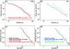 |
Fig. 6. Panel a: frequency distribution of duration for all events detected by ALMA (black solid curve) and for those with AIA counterparts, either 304 or 1600 Å, (red solid curve). The dashed black and dashed red lines represent the fitting of those distributions with power-law functions, while the purple and yellow curves indicate their fitting with exponential functions. Panel b: frequency distributions of duration for all events detected at 304 Å (solid blue) and 1600 Å (solid green) and their fittings with power-law functions (dashed blue and dashed green, respectively). Panels c and d: same as (a) and (b), respectively, but for the frequency distribution of maximum area. |
The frequency distributions represent number of events per unit of any given parameter. We note that all of these distributions can be fitted with power-law functions above a cutoff. In each case, a linear fit in logarithmic axes was performed that gave the power-law function parameters. The fitting range was determined automatically as the widest range of values that yielded mean error bars less than 10%. Each point within the fitting range was assigned with an uncertainty computed assuming Poisson statistics of the number of events in the histogram bins we used to calculate the frequency distribution. The propagation of these uncertainties yields uncertainties on the fitted power-law indices that are reported in Table 2.
The mean maximum areas of the events lie between 12.3 Mm2 and 15.5 Mm2. We note that these values were derived after we divided the apparent areas by μ. Our calculations together with their error bars indicate that the size of event blobs is similar in all three wavelengths and this result could be attributed to both the smoothing of the AIA data with the ALMA beam and the use of the ALMA-beam size spatial coherence detection criterion for all three datasets. The frequency distributions of event maximum areas were fitted with power-law functions extending from 6.5 Mm2 to about 75 Mm2. The power-law index for the ALMA events is higher than the indices for both the 304 Å and 1600 Å events, and (given the uncertainties involved) agrees with that for the ALMA events that had AIA counterparts. These values lie between those reported by Joulin et al. (2016) and Berghmans et al. (1998), who used AIA data in several passbands and 304 Å EIT data, respectively. There are no events with areas less than about 6.5 Mm2 as a result of the spatial coherence detection criterion that we used.
We quantified the average duration of the detected events by measuring their FWHM in the corresponding light curves (see Table 2). The frequency distributions of event durations are also power laws extending from 8, 12, and 24 s for the 3 mm, 304, and 1600 Å data, respectively, to about 100 s. The different low-end cutoffs reflect the different cadences and event detection schemes used for the three datasets (see Sect. 2). Overall the derived power-law indices are within the values reported in the literature (e.g., see Joulin et al. 2016 and references therein). It is also interesting that, again, the power-law index of the ALMA events that had AIA counterparts agrees with that of the general population of ALMA events if uncertainties are taken into account. We note, however, that the power-law fittings cannot account for the high-end values of the ALMA duration frequency distributions (see Fig. 6a). The situation changes if we fit these distributions with exponential functions (the relevant best-fit functions were of the form: frequency distribution ∝exp(−a ⋅ duration), where a = 0.087 and 0.082 s−1 for all and paired events, respectively) at the expense of obtaining relatively poor fits for the low-end values of the frequency distributions. Overall, the values of χ2 for the exponential fits are about 10% smaller than those of the power-law fits, which implies that the exponential fits have a slight edge over the power-law fits in the modeling of the ALMA duration frequency distributions.
The light curves of all events (e.g., see top row of Fig. 1, as well as those in Figs. 7–9) are gradual. Although the lack of ALMA data at two frequencies does not allow us to compute the spectral index of the millimeter-wavelength emission of the events, the gradual rise and fall of their light curves strongly suggests a thermal origin via the free-free mechanism. This behavior is in agreement with the results obtained by White et al. (1995) for transient brightenings detected at 17 GHz, but contradicts other studies of microwave data that reported the presence of nonthermal populations of electrons (e.g., Gary et al. 1997; Krucker et al. 1997; Nindos et al. 1999). However, quantitative calculations verify that only Mega-electron-volt-energy electrons can produce significant gyrosynchrotron emission at 3 mm (e.g., White & Kundu 1992).
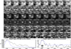 |
Fig. 7. A transient brightening detected both in 3 mm and 304 Å target 4 data. Row a: characteristic ALMA snapshots with field of view of 35″ × 35″; while row b shows the same snapshots after the subtraction of the average ALMA image. Rows c–f: same as rows a and b but for the 304 Å data (rows c and d), and the 1600 Å data (rows e and f). The white arrows indicate the transient brightening in the ALMA and 304 Å data. Bottom row: time profiles of the event emission at 3 mm (black curves) and 304 Å (blue curves), before (left panel) and after (right panel) our processing; the processed light curves show values above the background level. The 304 Å light curves are in arbitrary units, normalized to fit the vertical extent of the ALMA plots. |
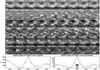 |
Fig. 8. Same as Fig. 7 for an event that was detected both in 3 mm and 1600 Å data. The layout of the figure is the same as that of Fig. 7 with the following exceptions: rows c and d correspond to 1600 Å data while rows e and f correspond to 304 Å data. The white arrows indicate the event at 3 mm and 1600 Å. In the bottom row the green curves show light curves from the 1600 Å data; these light curves are in arbitrary units, normalized to fit the vertical extent of the ALMA plots. |
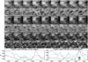 |
Fig. 9. Same as Fig. 7 for an event (number 48) that was detected in 3 mm data but did not show any conspicuous signature in AIA data. The layout of the figure is the same as that of Fig. 7 with the exception that in the bottom row the blue and green curves represent light curves from 304 Å and 1600 Å data, respectively, calculated from the pixels that correspond to the ALMA transient brightening. |
In Figs. 7–9 we present three characteristic events. The first event was detected in both ALMA and 304 Å data, the second was detected in both ALMA and 1600 Å, while the third appeared only in ALMA data with no compelling signature in the AIA databases. All events are so weak that they cannot be readily identified in the plain images, but their visual identification, as unresolved bright kernels, is possible after the subtraction of the temporally averaged image from each snapshot image. In all these figures the event component dominates the light curves over the residual oscillatory pattern with the exception of the 1600 Å and 304 Å light curves of Fig. 9; in the latter case this was natural because these light curves were calculated from pixels that did not belong to any detected AIA event. We note that although a local peak of the 304 Å light curve of Fig. 9 occurs close to the time of the 3 mm peak, it does not qualify as an event because it did not exceed the 2.5σ threshold.
4. Implications for chromospheric heating
In this section we present our estimates of the thermal energy supplied to the chromosphere by the ALMA transient brightenings. By doing so we certainly miss other potential carriers of energy, such as flows and waves, that might also be associated with such events. We assume that that their emission comes from the thermal free-free mechanism (see Sect. 3). We start from the following well-known expression for the thermal energy:
where Te is the electron temperature, k is the Boltzmann constant, and a filling factor of unity has been assumed. Assuming, further, that the electron density, Ne, and apparent volume, Vap, do not vary appreciably during the events, the extra energy, ΔEi, supplied to the chromosphere during the time interval between two consecutive images, i − 1 and i, is written as
where ΔTe, i = Te, i − Te, i − 1 is the difference of the electron temperature. Under the reasonable assumption that the energy release occurs during the rise time of the brightening, the total energy provided, E, is given as
where imax is the number of the image at which temperature reaches its maximum. The sum in Eq. (3) is obviously equal to the peak electron temperature, Te, max above background, Te, 0, that is, Te, max − Te, 0, so that, finally,

From the processed light curves of each event we obtained its maximum excess brightness temperature above background Tb, max − Tb, 0. In order to find the Te, max − Te, 0 which is required by Eq. (4) we need to know the optical depth, τ. To this end we used the results by Alissandrakis et al. (2017b) who, after they inverted the center-to-limb variation curve of full-disk data, found electron temperature values in the range 7250–7950 K, which were only 5% lower than those provided by the Fontenla et al. (1993) FAL C model. In that model the above electron temperatures correspond to heights from h1 ≈ 1775 km to h2 ≈ 1950 km. If we use that range of electron temperatures and the corresponding FAL C values for Ne, we find that our events occur in configurations in which the optical depth ranges from about 10 to 16, that is, they are optically thick. Therefore it is reasonable to use the excess brightness temperature above background from our corrected 3 mm light curves for the computation of the excess electron temperatures involved in Eq. (2).
For the evaluation of the energy budget we used the same FAL C electron density values as in the calculation of τ. For each event our calculations were done twice: first for the values of electron density corresponding to h1 and then for their values that correspond to h2.
Finally, we assume that the volume, Vap, can be estimated from the area, A, of the event through the equation Vap = A3/2, that is, we assume that the extent in height is comparable to the horizontal size. Our assumptions for constant electron density and filling factor f = 1 imply that the derived energies represent upper limits and as does the assumption about the vertical scale of the events, which should be comparable to the vertical extent of the chromosphere, an extent over which the plasma properties may change dramatically.
Our computations (see Table 3) yielded thermal energies ranging from (1.5 ± 0.1) × 1024 to (9.9 ± 2.0) × 1025 erg. The uncertainties come from the range of electron temperatures and densities used in each event calculations and from the root mean square (rms) of the distribution of apparent areas of the events. The lower-end values of the derived energies is consistent with the high-end limit of the nominal nanoflare energy (1024 erg). Furthermore, the range of computed energies falls within the cluster of values that have been reported in the literature: they are consistent with or smaller than the values reported by Krucker & Benz (1998; 8 × 1024 − 1.6 × 1026 erg), Berghmans et al. 1998; 5 × 1024 − 3 × 1027 erg), and Winebarger et al. (2013; 2.0 − 6.3 × 1024 erg). On the other hand, Aschwanden et al. (2000), Parnell & Jupp (2000), and Subramanian et al. (2018) reported energy ranges (5 × 10²³ − 5 × 1026 erg, 1023 − 1026 erg, and 0.3 − 30.0 × 1024 erg, respectively) whose low-end values are below the lowest energies we detected. Moreover, studies of active region weak transient brightenings report larger energies than ours (e.g., Shimizu 1995; 1025 − 1029 erg and Hannah et al. 2008; 1026 − 1030 erg).
Energy budgets of ALMA transient brightenings.
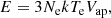
We also computed the frequency distribution (i.e., number of events per unit energy) of all ALMA transient brightenings as a function of their energy. The results for all ALMA events is given by the solid black curve of Fig. 10. The gray band shows the uncertainties in the frequency distribution which incorporate the error bars associated with both the energy calculations and the construction of the frequency distribution (see Sect. 3). For energies higher than 2.4 × 1024 erg (i.e., if we exclude the extreme low-end part of the computed energies) the frequency distribution of events can be fitted with a power-law function with index of 1.67 ± 0.05 (see the blue curve in Fig. 10). The derived power-law index is consistent with indices derived for RHESSI microflares (1.7; Hannah et al. 2008), AIA coronal brightenings (1.65–1.94; Joulin et al. 2016), and large flares observed by AIA (1.66; Aschwanden & Shimizu 2013).
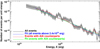 |
Fig. 10. Frequency distribution of all ALMA transient brightenings as a function of energy shown with black curve. The gray band represents the error bars discussed in Sect. 4. For energies > 2.4 × 1024 erg, the frequency distribution of events has been fitted with a power-law function with index of 1.67 (blue curve). The red curve corresponds to the frequency distribution vs. energy of only those ALMA events that have also been detected in AIA data (either 304 Å or 1600 Å). The green curve represents the fitting of that distribution with a power-law function with index of 1.65. |
In Fig. 10 the red curve shows the frequency distribution as a function of energy of only those ALMA events that had AIA counterparts (either 304 or 1600 Å). The minimum energy of that population was 2.6 × 1024 erg (i.e., the low-end energy values of the general population of events were missing, but the minimum energy of the population of paired events was close to the cutoff value used for the fitting of the frequency distribution of the general population of events) while its maximum energy was very similar to that of the general population of events. The frequency distribution of the paired events was fitted with a power-law function with index 1.65 ± 0.06, consistent with the power-law index derived for the general population of events.
From the total amount of energy of the detected events, the duration of observations in all six targets, and the area of the six fields of view, we calculated the resulted energy per unit area and time, which was about 1.9 ×10⁴ erg cm−2 s−1. This value is factors of 3.8 and 44 smaller than the power per unit area of the events studied by Krucker & Benz (1998) and Benz & Krucker (2002), respectively. It is also a factor of 4.6 smaller than the dissipation rate of magnetic energy per unit area in the quiet corona computed by Meyer et al. (2013). The total radiative losses from the quiet low chromosphere are on the order of 2 × 10⁶ erg cm−2 s−1, which is about one order of magnitude higher than the relevant quiet corona losses (e.g., see Withbroe & Noyes 1977). Therefore the energy supplied by the weak ALMA transient brightenings can account for only about 1% of the chromospheric radiative losses and about 10% of the coronal radiative losses.
The results of the total thermal energy content of the configurations that hosted the transient brightenings depend on the event selection criteria. If less restrictive criteria are adopted, both the number and energy content of the selected events increase. For example, we estimated the energy content of the ALMA events detected by using both a 2.3σ and a 2.1σ threshold above the average intensity for the light curves and by relaxing the spatial coherence criterion in the latter case. The 2.1σ threshold was selected because below this threshold, the power-law form of the frequency distribution functions disappears. The results appear in Table 3. In the least restrictive case of the 2.1σ threshold, the number of detected events increased by a factor of about 9; the low-end limit of their energy range dropped to (4.0 ± 1.5) × 1023 erg, while the power-law index of the frequency distribution of the events versus their energy became 1.88 ± 0.02, and their power to unit area increased to 3.3 × 10⁴ erg cm−2 s−1. Interestingly, the characteristics of the energy distribution of the events with AIA counterparts did not change very much (see Table 3).
5. Summary and conclusions
In this article we present the first systematic survey for transient brightenings in the quiet Sun using ALMA observations at 3 mm. Compared to the more usual EUV/soft X-ray (SXR) surveys, the ALMA data have the advantage of the superior cadence and the easier derivation of the physical properties of the detected events. Furthermore, they probe cooler and denser chromospheric plasma, which is not accessible with EUV/SXR observations.
On the other hand, any attempt to search ALMA 3 mm data for transient brightenings needs to confront the ubiquitous presence of the p-mode oscillations, which could exhibit amplitudes as high as 350 K in individual pixels (Patsourakos et al. 2020). To this end, an important component of our event detection algorithm was the identification and removal of oscillations from the light curves of individual pixels. There was a slight increase of residual oscillation power toward the limb, and thus there is no surprise that we detected a weak increase of the maximum brightness temperature of the event pixels toward the limb as well.
Using our selection criteria (see Sect. 2) we were able to able to detect 184 events in the six 87″ × 87″ targets, each one observed for 10 min. All events were of the gradual rise and fall type, strongly suggesting a thermal origin. The average maximum brightness temperature of the detected events ranged from about 70 K to more than 500 K above the average intensity. The mean values of their maximum area and duration were 12.3 Mm2 and 51.1 s, respectively, with a weak preference (∼68%) occurring at network boundaries than in cell interiors. The frequency distributions of both parameters followed power-law functions with indices of 2.73 and 2.35, respectively; we note though that an exponential function provided a slightly better fit to the frequency distribution of duration. These values are broadly consistent with previous reports of these quantities from EUV/SXR observations.
The detection of ALMA transient brightenings was complemented with the search for transient brightenings in the corresponding AIA data obtained at 304 and 1600 Å. We detected 199 events in 304 Å and 633 in 1600 Å. As a consquence of the smoothing of the AIA data with the ALMA beam and the usage of ALMA beam-size patches of adjacent pixels for the spatial coherence criterion, the size of the events were similar in all three wavelengths. Furthermore, there was a weak preference (∼57%) for the 1600 Å events to occur in cell interiors, which could imply that part of the oscillatory strength was not removed.
Only a small fraction of ALMA events had 304 Å and 1600 Å counterparts (18 and 14), respectively. The basic properties of the paired ALMA events were consistent with those of the general population of ALMA events with the exception that their energy distribution did not reach the low-end values of the corresponding distribution of the general population.
Regarding the question of why most 3 mm events were not detected at 304 Å or 1600 Å, and vice versa, we point out that in addition to differences in sensitivity, which need to be addressed in a future work, the three datasets probe different ranges of temperatures (or equivalently the corresponding emissions form at different heights; see Alissandrakis 2019). The 3 mm events probe cool chromospheric material whose temperature may not increase sufficiently to give rise to 304 Å emission. On the other hand, the 304 Å or 1600 Å events may not be strong enough to energize the atmospheric layers that are probed by ALMA. Furthermore, all three wavelengths should be optically thick in the context of our study; therefore it is perhaps not surprising that ALMA transients, seen higher in the chromosphere, do not correlate well with those that occur lower down because we do not see down to those heights at 3 mm.
The thermal energies supplied to the chromosphere by the ALMA events are between 1.5 × 1024 and 9.9 × 1025 erg and their frequency distribution versus energy follows a power-law function with index of 1.67. The ALMA events that had AIA counterparts lack the low-end energy values of the general population of events and follow a power-law distribution with index of 1.65. The power per unit area supplied by the ALMA events can account for only 1% of the chromospheric radiative losses or equivalently 10% of the coronal losses.
Of course any calculation of the energy budget of transient brightenings is sensitive to the detection criteria that have been employed. In our case using the less restrictive criteria, we derived results that did not change the basic conclusion that the energy content of the ALMA transient brightenings is not sufficient to heat the chromosphere. This is the case even though the number of detected events increased and the calculated energy range extended down to somehow lower energies. We note, however, that in light of the fact that the 3 mm emission should be optically thick, we probably detected transient brightenings from a thin layer of the chromosphere of only a few hundred kilometer in thickness. We speculate that if we were to add up a truly volumetric sample of transients occurring at all heights their contribution to heating might increase significantly.
Our observations were carried out with most compact array configuration available using ALMA at the cost of inferior spatial resolution; we speculate that the use of higher spatial resolution ALMA observations could yield the detection of smaller and energetically weaker events that could lead to steeper power-law functions for the frequency distribution of events. Observations at ALMA Band 1 at 7.25 mm (whenever that will become available for solar observing), where the impact of oscillations is expected to be smaller, could also facilitate the detection of more events. Another item for future research are the physical mechanisms that cause the transient brightenings that we detected. Previous publications propose that transient chromospheric temperature increases that may be associated with the observed brightenings in millimeter wavelengths could result from acoustic (Carlsson & Stein 1995; Wedemeyer et al. 2004) or magnetoacoustic shocks (Rouppe van der Voort et al. 2007). These and possibly other alternatives should be checked against the properties of the transient brightenings that we detected.
Acknowledgments
We thank the referee for his/her comments which led to improvement of the paper. This paper makes use of the following ALMA data: ADS/JAO.ALMA2016.1.00572.S. ALMA is a partnership of ESO (representing its member states), NSF (USA) and NINS (Japan), together with NRC (Canada) and NSC and ASIAA (Taiwan), and KASI (Republic of Korea), in cooperation with the Republic of Chile. The Joint ALMA Observatory is operated by ESO, AUI/NRAO and NAOJ.
References
- Alissandrakis, C. E. 2019, Sol. Phys., 294, 161 [Google Scholar]
- Alissandrakis, C. E., Nindos, A., Patsourakos, S., et al. 2015, A&A, 582, A52 [NASA ADS] [CrossRef] [EDP Sciences] [Google Scholar]
- Alissandrakis, C. E., Koukras, A., Patsourakos, S., et al. 2017a, A&A, 603, A95 [NASA ADS] [CrossRef] [EDP Sciences] [Google Scholar]
- Alissandrakis, C. E., Patsourakos, S., Nindos, A., & Bastian, T. S. 2017b, A&A, 605, A78 [NASA ADS] [CrossRef] [EDP Sciences] [Google Scholar]
- Aschwanden, M. J., & Shimizu, T. 2013, ApJ, 776, 132 [NASA ADS] [CrossRef] [Google Scholar]
- Aschwanden, M. J., Tarbell, T. D., Nightingale, R. W., et al. 2000, ApJ, 535, 1047 [NASA ADS] [CrossRef] [Google Scholar]
- Bastian, T. S., Chintzoglou, G., De Pontieu, B., et al. 2017, ApJ, 845, L19 [NASA ADS] [CrossRef] [Google Scholar]
- Benz, A. O., & Krucker, S. 1998, Sol. Phys., 182, 349 [NASA ADS] [CrossRef] [Google Scholar]
- Benz, A. O., & Krucker, S. 1999, A&A, 341, 286 [NASA ADS] [Google Scholar]
- Benz, A. O., & Krucker, S. 2002, ApJ, 568, 413 [NASA ADS] [CrossRef] [Google Scholar]
- Berghmans, D., Clette, F., & Moses, D. 1998, A&A, 336, 1039 [NASA ADS] [Google Scholar]
- Brajša, R., Sudar, D., Benz, A. O., et al. 2018, A&A, 613, A17 [NASA ADS] [CrossRef] [EDP Sciences] [Google Scholar]
- Brooks, D. H., & Warren, H. P. 2012, ApJ, 760, L5 [CrossRef] [Google Scholar]
- Carlsson, M., & Stein, R. F. 1995, ApJ, 440, L29 [NASA ADS] [CrossRef] [Google Scholar]
- Crosby, N. B., Aschwanden, M. J., & Dennis, B. R. 1993, Sol. Phys., 143, 275 [NASA ADS] [CrossRef] [Google Scholar]
- De Pontieu, B., McIntosh, S. W., Hansteen, V. H., et al. 2009, ApJ, 701, L1 [NASA ADS] [CrossRef] [Google Scholar]
- Dillon, J. D. B., Kirk, M. S., Reale, F., et al. 2019, ApJ, 871, 133 [Google Scholar]
- Fontenla, J. M., Avrett, E. H., Loeser, R. 1993, ApJ, 406, 319 [NASA ADS] [CrossRef] [Google Scholar]
- Gary, D. E., Hartl, M., & Shimizu, T. 1997, ApJ, 477, 958 [NASA ADS] [CrossRef] [Google Scholar]
- Hannah, I. G., Christie, S., Krucker, S., et al. 2008, ApJ, 677, 704 [NASA ADS] [CrossRef] [Google Scholar]
- Hara, H., Watanabe, T., Harra, L. K., et al. 2008, ApJ, 678, L6 [NASA ADS] [CrossRef] [Google Scholar]
- Hinode Review Team (Al-Janabi, K., et al.) 2019, PASJ, 71, R1 [CrossRef] [Google Scholar]
- Hudson, H. S. 1991, Sol. Phys., 133, 357 [Google Scholar]
- Jafarzadeh, S., Wedemeyer, S., Szydlarski, M., et al. 2019, A&A, 622, A150 [NASA ADS] [CrossRef] [EDP Sciences] [Google Scholar]
- Joulin, V., Buchlin, E., Solomon, J., et al. 2016, A&A, 591, A148 [CrossRef] [EDP Sciences] [Google Scholar]
- Katsukawa, Y., & Tsuneta, S. 2001, ApJ, 557, 343 [NASA ADS] [CrossRef] [Google Scholar]
- Klimchuk, J. A. 2012, J. Geophys. Res., 117, A12102 [NASA ADS] [CrossRef] [Google Scholar]
- Krucker, S., & Benz, A. O. 1998, ApJ, 501, L213 [NASA ADS] [CrossRef] [Google Scholar]
- Krucker, S., Benz, A. O., Bastian, T. S., et al. 1997, ApJ, 488, 499 [Google Scholar]
- Leenaarts, J., Pereira, T. M. D., Carlsson, M., et al. 2013, ApJ, 772, 90 [NASA ADS] [CrossRef] [Google Scholar]
- Lemen, J. R., Title, A. M., Akin, D. J., et al. 2012, Sol. Phys., 275, 17 [NASA ADS] [CrossRef] [Google Scholar]
- Loukitcheva, M. A., White, S. M., & Solanki, S. K. 2019, ApJ, 877, L26 [NASA ADS] [CrossRef] [Google Scholar]
- Martinez-Sykora, J., De Pontieu, B., de la Cruz Rodriguez, H., et al. 2020, ApJ, 891, L8 [CrossRef] [Google Scholar]
- Marsh, A. J., Smith, D. M., Glesener, L., et al. 2018, ApJ, 864, 5 [NASA ADS] [CrossRef] [Google Scholar]
- Meyer, K. A., Sabol, J., Mackay, D. H., et al. 2013, ApJ, 770, L18 [NASA ADS] [CrossRef] [Google Scholar]
- Molnar, M. E., Reardon, K. P., Chai, Y., et al. 2019, ApJ, 881, 99 [NASA ADS] [CrossRef] [Google Scholar]
- Nindos, A., Kundu, M. R., & White, S. M. 1999, ApJ, 513, 983 [Google Scholar]
- Nindos, A., Alissandrakis, C. E., Bastian, T. S., et al. 2018, A&A, 619, L6 [NASA ADS] [CrossRef] [EDP Sciences] [Google Scholar]
- Parker, E. N. 1988, ApJ, 330, 474 [Google Scholar]
- Parnell, C. E., & Jupp, P. E. 2000, ApJ, 529, 554 [NASA ADS] [CrossRef] [Google Scholar]
- Patsourakos, S., Alissandrakis, C. E., Nindos, A., et al. 2020, A&A, 634, A86 [NASA ADS] [CrossRef] [EDP Sciences] [Google Scholar]
- Peter, H., Tian, H., Curdt, W., et al. 2014, Science, 346, 1255726 [NASA ADS] [CrossRef] [Google Scholar]
- Ramesh, R., Kathiravan, C., Barve, I. V., et al. 2010, ApJ, 719, L41 [NASA ADS] [CrossRef] [Google Scholar]
- Régnier, S., Alexander, C. E., Walsh, R. W., et al. 2014, ApJ, 784, 134 [NASA ADS] [CrossRef] [Google Scholar]
- Rodger, A. S., Labrosse, N., Wedemeyer, S., et al. 2019, ApJ, 875, 163 [NASA ADS] [CrossRef] [Google Scholar]
- Roerink, G. J., Menenti, M., & Verhoef, W. 2000, Int. J. Rem. Sens., 21, 1911 [NASA ADS] [CrossRef] [Google Scholar]
- Rouppe van der Voort, L. H. M., De Pontieu, B., Hansteen, V. H., et al. 2007, ApJ, 660, L169 [NASA ADS] [CrossRef] [Google Scholar]
- Rouppe van der Voort, L. H. M., Rutten, R. J., & Vissers, G. J. 2016, A&A, 592, A100 [NASA ADS] [CrossRef] [EDP Sciences] [Google Scholar]
- Saint-Hilaire, P., Vilmer, N., & Kerdraon, A. 2013, ApJ, 762, 60 [NASA ADS] [CrossRef] [Google Scholar]
- Selhorst, C. L., Simões, P. J. A., Brajša, R., et al. 2019, ApJ, 871, 45 [NASA ADS] [CrossRef] [Google Scholar]
- Shetye, J., Shelyag, S., Reid, A. L., et al. 2018, MNRAS, 479, 3274 [Google Scholar]
- Shibasaki, K., Alissandrakis, C. E., & Pohjolainen, S. 2011, Sol. Phys., 273, 309 [Google Scholar]
- Shimizu, T. 1995, PASJ, 47, 251 [NASA ADS] [Google Scholar]
- Shimizu, T., Tsuneta, S., Acton, L. W., et al. 1994, ApJ, 422, 906 [NASA ADS] [CrossRef] [Google Scholar]
- Shimojo, M., Bastian, T. S., Hales, A. S., et al. 2017a, Sol. Phys., 292, 87 [Google Scholar]
- Shimojo, M., Hudson, H. S., White, S. M., et al. 2017b, ApJ, 841, L5 [NASA ADS] [CrossRef] [Google Scholar]
- Subramanian, S., Kashyap, V. L., Tripathi, D., et al. 2018, A&A, 615, A47 [CrossRef] [EDP Sciences] [Google Scholar]
- Suresh, A., Sharma, R., Oberoi, D., et al. 2017, ApJ, 843, 19 [CrossRef] [Google Scholar]
- Terzo, S., Reale, F., Miceli, M., et al. 2011, ApJ, 736, 111 [NASA ADS] [CrossRef] [Google Scholar]
- Tian, H., DeLuca, E. E., Cranmer, S. R., et al. 2014, Science, 346, 1255711 [Google Scholar]
- Ulyanov, A. S., Bogachev, S. A., Reva, A. A., et al. 2019, Astron. Lett., 45, 248 [CrossRef] [Google Scholar]
- Viall, N. M., & Klimchuk, J. A. 2012, ApJ, 753, 35 [NASA ADS] [CrossRef] [Google Scholar]
- Vissers, G. J. M., Rouppe van der Voort, L. H. M., Rutten, R. J., et al. 2015, ApJ, 812, 1 [Google Scholar]
- Yokoyama, T., Shimojo, M., Okamoto, T. J., et al. 2018, ApJ, 863, 96 [NASA ADS] [CrossRef] [Google Scholar]
- Warren, H. P., Ugarte-Urra, I., Brooks, D. H., et al. 2007, PASJ, 59, S675 [NASA ADS] [Google Scholar]
- Wedemeyer, S., Freytag, B., Steffen, M., et al. 2004, A&A, 414, 1121 [NASA ADS] [CrossRef] [EDP Sciences] [Google Scholar]
- Wedemeyer, S., Bastian, T., Brajša, R., et al. 2016, Space Sci. Rev., 200, 1 [NASA ADS] [CrossRef] [Google Scholar]
- Wedemeyer, S., Szydlarski, M., Jafarzadeh, S., et al. 2020, A&A, 635, A71 [CrossRef] [EDP Sciences] [Google Scholar]
- White, S. M., & Kundu, M. R. 1992, Sol. Phys., 141, 347 [NASA ADS] [CrossRef] [Google Scholar]
- White, S. M., Kundu, M. R., Shimizu, T., et al. 1995, ApJ, 450, 435 [NASA ADS] [CrossRef] [Google Scholar]
- White, S. M., Loukitcheva, M., & Solanki, S. K. 2006, A&A, 456, 697 [NASA ADS] [CrossRef] [EDP Sciences] [Google Scholar]
- White, S. M., Iwai, K., Phillips, N. M., et al. 2017, Sol. Phys., 292, 88 [NASA ADS] [CrossRef] [Google Scholar]
- Winebarger, A. R., Walsh, R. W., Moore, R., et al. 2013, ApJ, 771, 21 [NASA ADS] [CrossRef] [Google Scholar]
- Withbroe, G. L., & Noyes, R. W. 1977, ARA&A, 15, 363 [NASA ADS] [CrossRef] [Google Scholar]
All Tables
All Figures
|
Fig. 1. Top row: light curves of a target 3 single pixel showing transient brightening before (a) and after (d) the processing described in Sect. 2. In this and subsequent light-curve displays, the arrows indicate the times in which the intensity exceeds the 2.5σ threshold above average. Middle row: same as top row for a pixel that did not show transient brightening. The curve in panel b has been displaced by −300 K. Bottom row: panel c shows the power spectra deduced from light curves (a) and (b), while panel f shows the power spectra deduced from light curves (d) and (e). |
| In the text | |
|
Fig. 2. Top: ratio of the target 5 “event pixels” with respect to the number of pixels of the whole field of view (expressed in percentage) as a function of the σ multiplication factor that determines the threshold for the detection of transient brightenings. No additional spatial coherence detection criteria have been applied for the production of these results. Bottom: same quantity as top curve but now computed as a function of the minimum number of adjacent pixels on top of the 2.5σ multiplication factor. |
| In the text | |
|
Fig. 3. Histograms of maximum brightness temperature above the background of the selected event pixels for all targets. |
| In the text | |
|
Fig. 4. Top: average maximum brightness temperature of the selected event pixels in each target as a function of μ. The error bars denote the standard deviation of the corresponding distributions. The red line shows the linear-squares fit to the measurements. Bottom: same as top, but for the average maximum residual oscillation power. |
| In the text | |
|
Fig. 5. Display of the selected pixels that correspond to transient brightenings in 1600 Å (green), 3 mm (red), and 304 Å (blue) target 4 data. Top row: all events detected at a given wavelength are denoted. Bottom row: panels e and f show only the events that appear both at 3 mm and 1600 Å, respectively, while panels g and h show only the events that appear both at 3 mm and 304 Å, respectively. In each panel the relevant average image is shown as background. |
| In the text | |
|
Fig. 6. Panel a: frequency distribution of duration for all events detected by ALMA (black solid curve) and for those with AIA counterparts, either 304 or 1600 Å, (red solid curve). The dashed black and dashed red lines represent the fitting of those distributions with power-law functions, while the purple and yellow curves indicate their fitting with exponential functions. Panel b: frequency distributions of duration for all events detected at 304 Å (solid blue) and 1600 Å (solid green) and their fittings with power-law functions (dashed blue and dashed green, respectively). Panels c and d: same as (a) and (b), respectively, but for the frequency distribution of maximum area. |
| In the text | |
|
Fig. 7. A transient brightening detected both in 3 mm and 304 Å target 4 data. Row a: characteristic ALMA snapshots with field of view of 35″ × 35″; while row b shows the same snapshots after the subtraction of the average ALMA image. Rows c–f: same as rows a and b but for the 304 Å data (rows c and d), and the 1600 Å data (rows e and f). The white arrows indicate the transient brightening in the ALMA and 304 Å data. Bottom row: time profiles of the event emission at 3 mm (black curves) and 304 Å (blue curves), before (left panel) and after (right panel) our processing; the processed light curves show values above the background level. The 304 Å light curves are in arbitrary units, normalized to fit the vertical extent of the ALMA plots. |
| In the text | |
|
Fig. 8. Same as Fig. 7 for an event that was detected both in 3 mm and 1600 Å data. The layout of the figure is the same as that of Fig. 7 with the following exceptions: rows c and d correspond to 1600 Å data while rows e and f correspond to 304 Å data. The white arrows indicate the event at 3 mm and 1600 Å. In the bottom row the green curves show light curves from the 1600 Å data; these light curves are in arbitrary units, normalized to fit the vertical extent of the ALMA plots. |
| In the text | |
|
Fig. 9. Same as Fig. 7 for an event (number 48) that was detected in 3 mm data but did not show any conspicuous signature in AIA data. The layout of the figure is the same as that of Fig. 7 with the exception that in the bottom row the blue and green curves represent light curves from 304 Å and 1600 Å data, respectively, calculated from the pixels that correspond to the ALMA transient brightening. |
| In the text | |
|
Fig. 10. Frequency distribution of all ALMA transient brightenings as a function of energy shown with black curve. The gray band represents the error bars discussed in Sect. 4. For energies > 2.4 × 1024 erg, the frequency distribution of events has been fitted with a power-law function with index of 1.67 (blue curve). The red curve corresponds to the frequency distribution vs. energy of only those ALMA events that have also been detected in AIA data (either 304 Å or 1600 Å). The green curve represents the fitting of that distribution with a power-law function with index of 1.65. |
| In the text | |
Current usage metrics show cumulative count of Article Views (full-text article views including HTML views, PDF and ePub downloads, according to the available data) and Abstracts Views on Vision4Press platform.
Data correspond to usage on the plateform after 2015. The current usage metrics is available 48-96 hours after online publication and is updated daily on week days.
Initial download of the metrics may take a while.