| Issue |
A&A
Volume 636, April 2020
|
|
|---|---|---|
| Article Number | A17 | |
| Number of page(s) | 15 | |
| Section | Interstellar and circumstellar matter | |
| DOI | https://doi.org/10.1051/0004-6361/201937157 | |
| Published online | 08 April 2020 | |
Modeling the magnetized Local Bubble from dust data
1
Institute of Astrophysics, Foundation for Research and Technology-Hellas,
71110
Heraklion,
Greece
2
Department of Physics, University of Crete,
70013
Heraklion,
Greece
e-mail: This email address is being protected from spambots. You need JavaScript enabled to view it.
3
Institut de Recherche en Astrophysique et Planétologie (IRAP), CNRS, Université de Toulouse, CNRS,
9 avenue du Colonel Roche, BP 44346,
31028
Toulouse Cedex 4,
France
4
École normale supérieure/LERMA, Observatoire de Paris, Sorbonne Université, Université PSL, CNRS,
Paris, France
5
GEPI, Observatoire de Paris, PSL University, CNRS,
5 place Jules Janssen,
92190
Meudon, France
Received:
21
November
2019
Accepted:
17
February
2020
Abstract
The Sun is embedded in the so-called Local Bubble (LB) – a cavity of hot plasma created by supernova explosions and surrounded by a shell of cold, dusty gas. Knowing the local distortion of the Galactic magnetic field associated with the LB is critical for the modeling of interstellar polarization data at high Galactic latitudes. In this his paper, we relate the structure of the Galactic magnetic field on the LB scale to three-dimensional (3D) maps of the local interstellar medium (ISM). First, we extracted the geometry of the LB shell, its inner surface, in particular from 3D dust extinction maps of the local ISM. We expanded the shell inner surface in spherical harmonics, up to a variable maximum multipole degree, which enabled us to control the level of complexity for the modeled surface. Next, we applied an analytical model for the ordered magnetic field in the shell to the modeled shell surface. This magnetic field model was successfully fitted to the Planck 353 GHz dust polarized emission maps over the Galactic polar caps. For each polar cap, the direction of the mean magnetic field derived from dust polarization (together with the prior that the field points toward longitude 90° ± 90°) is found to be consistent with the Faraday spectra of the nearby diffuse synchrotron emission. Our work presents a new approach to modeling the local structure of the Galactic magnetic field. We expect our methodology and our results to be useful both in modeling the local ISM as traced by its different components and in modeling the dust polarized emission, which is a long-awaited input for studies of the polarized foregrounds for cosmic microwave background.
Key words: submillimeter: ISM / dust, extinction / ISM: magnetic fields / ISM: structure / cosmic background radiation / polarization
© ESO 2020
1 Introduction
The interstellar medium (ISM) that surrounds the Sun out to a radius on the order of 100−300 pc is known to have an unusually low atomic gas density of nHI ≲ 0.1 cm−3 (Cox & Reynolds 1987). This rarefied interstellar region is filled with a soft X-ray emitting plasma, as confirmed by the latest measurements and by recent analyses that take the heliospheric contribution to the soft X-ray background into account (Puspitarini et al. 2014; Galeazzi et al. 2014; Snowden et al. 2015; Liu et al. 2017). This so-called Local Cavity, also known as the Local Bubble (LB), is bounded by a shell of cold neutral gas and dust.
The LB was most likely created by supernova explosions that occurred over the past 10−15 Myr (Maíz-Apellániz 2001; Breitschwerdt et al. 2016). According to these authors, the progenitors of these supernovae belonged to stellar currents moving near the Galactic plane (within about 50 pc) and whose surviving members are probably part of the Scorpius-Centaurus (Sco-Cen) OB association. As discussed by Maíz-Apellániz (2001), backwards extrapolations of the trajectories of Sco-Cen OB association members in the Local Standard of Rest (LSR) show that the positions of the supernovae that exploded in the past 10 Myr fall outside, albeit very close to, the present boundary of the LB. If these supernovae are indeed located at the origin of the LB, one would have expected the weighted mean of their positions to be close to the center of the LB. However, this expectation implicitly relies on the assumptions that the local ISM (including the LB) moves exactly at the same velocity as the LSR and that the expansion motions driven by the explosions are isotropic, neither condition of which is actually satisfied. In reality, the local ISM is believed to move at a velocity of ≃15 km s−1 with respect to the LSR (e.g., Gry & Jenkins 2014), corresponding to a displacement of ≃150 pc in 10 Myr. In addition, large-scale density and pressure gradients in the local ISM must have favored expansion in certain directions, typically, away from the Galactic plane and towards the outer Galaxy. For instance, Maíz-Apellániz (2001) suggested that pressure imbalance between a large molecular complex in the Galactic Center direction and a pre-existent rarefied volume in the opposite direction may have shifted the LB center away from the mean explosion center; a realistic pressure-driven drift at a few km s−1 would be large enough to create a displacement ~50 pc in 10 Myr. Altogether, the present LB center could be offset by as much as ~200 pc from the sites of the explosions that occurred 10 Myr ago.
Global hydrodynamic and magneto-hydrodynamic models of the Galactic disk subjected to the effect of supernova explosions have been developed and a fraction of the computed cavities can match, at some stage, the characteristics (size, temperature, density range, and ion abundances) of the LB (see, e.g., de Avillez & Breitschwerdt 2009). More directly, thepresent shape and size of the LB can be extracted from three-dimensional (3D) maps of the dusty ISM surrounding the Sun (e.g., Green et al. 2019; Lallement et al. 2019, hereafter L19; Leike & Enßlin 2019, hereafter LE19). In addition to being interesting in its own right, determining and modeling the geometry of the LB is expected to be useful to model the interstellar density distribution in our Galactic vicinity, to constrain the expansion motions driven by the supernova explosions that created the LB, and to model the local Galactic magnetic field.
Several studies have demonstrated that the magnetic field in the local ISM does not follow the large-scale Galactic magnetic field (e.g. Heiles 1998; Leroy 1999; Santos et al. 2011; Frisch et al. 2012; Berdyugin et al. 2014; Gontcharov & Mosenkov 2019). For the first time, Alves et al. (2018, hereafter A18) quantified the association between the LB and the local magnetic field distortion. They developed an analytical model for the ordered magnetic field in the LB shell, which they assumed to be very thin and to result from purely radial expansion motions. Approximating the shape of the shell as a spheroid, A18 fitted their magnetic field model to the measured Planck dust polarized emission in the Galactic polar caps (|b| > 60°), where the contribution from the magnetized LB shell was expected to be dominant compared to the contribution from the large-scale Galactic magnetic field. Recently, Skalidis & Pelgrims (2019) were able to confirm this expectation: by comparing the dust polarized emission at 353 GHz with starlight optical polarization, they showed that the 353 GHz polarized sky is dominated at high Galactic latitudes by a dusty and magnetized structure extending from about 200 to 300 pc from the Sun. Thus, an accurate modeling of the magnetic field in the LB shell becomes an important milestone towards a comprehensive 3D modeling of the large-scale Galactic magnetic field, which, in turn, is critical for the physical characterization of the Galactic polarized foregrounds to the Cosmic Microwave Background (CMB).
In this paper, we develop a physically motivated approach to model the Galactic dust polarized emission in the Galactic polar caps. We infer the geometry of the LB shell directly from observational data. We then describe the shell geometry in mathematical terms in order to be able to study the local perturbation of the Galactic magnetic field associated with the formation of the LB. In that sense, our paper follows up and improves on the modeling of the magnetized LB shell proposed by A18. We also satisfactorily provide the first self-consistent physical model of the dust polarized sky at high Galactic latitudes using actual 3D data.
Our work contains two main parts, structured as follows. In Sect. 2, we extract the location and shape of the LB shell from 3D extinction maps and we provide a mathematical model, in terms of spherical harmonics, for the shell inner surface. We quantitatively compare the modeled surfaces obtained from the L19 and LE19 extinction maps both with each other and with the shape of the Local Hot Bubble (LHB) derived from X-ray emission data. In Sect. 3, we apply the magnetic field model of A18 to our shell inner surface, and we constrain this model by fitting it to the Planck dust polarized emission in the Galactic polar caps. We also test the stability of our results for the magnetic field and, therefore, for the dust polarized emission against several sources of uncertainty. Finally, we compare the best-fit magnetic fields derived with our approach to those from simpler models, and we confront our results to those of Faraday tomographic studies of the local ISM. Section 4 summarizes the work carried in this paper and presents some perspectives.
2 Geometry of the LB shell
2.1 Data set
In recent years, a growing number of 3D maps of the dusty Galactic space surrounding the Sun have been produced (see, e.g., the introduction of L19 for an exhaustive review). These data sets were made possible thanks to large photometric and spectroscopic surveys such as 2MASS, Pan-STARRS, SDSS/ APOGEE, accurate parallax measurements from Gaia, for example, and elaborate inversion techniques (e.g., see Green et al. 2019; L19; LE19 and references therein). Spectroscopic data improve the quality of the maps in different ways. Stellar spectral features constrain stellar types, and, in turn, extinction estimates. Absorption by gaseous species (e.g., Diffuse Interstellar Bands) can be used directly for mapping (see, e.g., Farhang et al. 2019 or used as proxies for dust extinction and merged with photometric determinations (Capitanio et al. 2017). To date, the latest products corresponding to large Galactic volumes are those presented in the first three aforementioned papers. Every 3D map comes with its own set of characteristics (covered volume, resolution, etc.) and with the strengths and weaknesses from either or both of the applied data sets and inversion methods.
In this work, we rely on 3D dust density maps to model the geometry of the LB shell. As discussed further in Sect. 2.4, we find that the most suitable available 3D map to perform our analysis is the map of L19, which is the only publicly available map that covers, in all directions, a volume large enough to contain the entire LB.
L19 constructed a 3D map of dust reddening based on Gaia DR2 photometric data combined with 2MASS measurements to derive extinction towards stars that possess accurate photometry and relative uncertainties in DR2 parallaxes smaller than 20%. They applied a hierarchical inversion algorithm which includes spatial correlation and which is adapted to large data sets and to an inhomogeneous target distribution. The resulting map is delivered on a Cartesian grid with voxel size of (5 pc)3. It covers a volume of [6.0 × 6.0 × 0.8] kpc3 centered on the Sun with the largest extent in the Galactic disk. The maximal spatial resolution achieved in that iterative inversion process is 25 pc. We refer the reader to the aforementioned paper for further details regarding the map-making process, the map itself and the description of the different data sets it relies on.
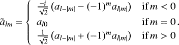
In Fig. 1, we show three crosscuts of the solar neighborhood according to the 3D dust extinction map of L19. This map gives the differential extinction,  (with r the distanceto the Sun), which we implicitly assume to be a proxy for the gas density. These crosscuts show the XY, XZ and YZ planes, where the X axis points from the Sun to the Galactic center at Galactic longitude l = 0°, the Y axis points towards l = 90° and the Z axis points to the North Galactic pole at Galactic latitude b = 90°. The LB cavity clearly stands out in this triptych.
Throughout this paper, we assume that the LB cavity results from supernova explosions, which shocked and swept up the ambient interstellar matter together with the frozen-in magnetic field. It is the layer of swept-up matter between the cavity and the surrounding ISM that we call the shell of the LB. In this section, we provide simple, but realistic, models of the shape of this shell.
2.2 Method
2.2.1 Inner and outer surfaces of the LB shell
To determine the geometry of the LB shell, we chose to rely on a criterion that is based on relative, rather than absolute, values of the reconstructed dust density. The procedure should be carried out automatically through the full data set. Our method can be described asfollows.
To begin with, we draw lines of sight originating from the Sun and running outwards with a radial sampling step of 2.5 pc. We perform the angular sampling according to a HEALPix tessellation of the celestial sphere (Górski et al. 2005). We set the Nside parameter to 128, providing an angular resolution of about 27′.5. Out to the 400 pc radial distance that we probe, the 3D extinction map is therefore well over-sampled and we do not miss material in the line-of-sight cones. To each node of our spherical grid, we assign a value derived from the 3D extinction map. Because the latter utilizes a uniform Cartesian grid, we need to convert from Cartesian to spherical coordinates. Here, we rely on a linear interpolation over the nearest neighbors of the Cartesian grid. For each line of sight, we thus obtain a radial profile of the differential extinction,  . The interpolation process induces spurious noise in the differential extinction curves. To eliminate this noise, we smooth these curves using a one-dimensional Gaussian smoothing kernel, with a standard deviation of 25 pc. This value corresponds to the maximum resolution of the 3D extinction map of L19. In Fig. 2, we show ten differential extinction curves randomly chosen in the XY plane of the Galaxy.
For each line of sight, we compute the first and second derivatives of  with respect to r. We then define the radius of the inner surface of the LB shell, rinner, as the distance to the first (closest to the Sun) inflection point, where the curve changes from convex to concave, that is, the first point at which
  . A cursory look at Fig. 1, particularly at the first quadrants of the left and right panels, reveals localized dust structures which are most likely unrelated to the LB shell and, therefore, should be ignored. The iterative procedure described in Sect. 2.2.2 makes it possible to bypass these dust structures and prevent them from biasing the determination of the shell inner surface.
Similarly, we locate the radius of the outer surface of the LB shell, router, at the second inflection point, wherethe  curve changes from concave to convex. Because of the complex dust density distribution in the ISM, especially in the Galactic disk, we find that our derived router is not reliable in some places1. For this reason, we focus on the modeling of the inner surface in the next subsection.
We apply the above method to the 3D extinction map of L19. The result is shown in the triptych of Fig. 3, where the inner and outer surfaces of the LB shell are plotted in red and green, respectively. Figure 3conveys a good sense of the complex geometry of the LB shell. An intervening cloud can be spotted towards (l, b) ≈ (0°, − 50°) in the fourth quadrant of the middle panel. It also emerges from Fig. 3 that the shell is relatively thick (ranging from 50 to 150 pc) and, more crucially with regard to our study, present all around the cavity, including the area towards the Galactic polar caps (|b|≥ 60°). This was not immediately obvious from the 3D extinction map alone, where the LB looks more like an open chimney. Towards the polar caps, the LB shell extends roughly from 200 to 300 pc, in agreement with the conclusion reached by Skalidis & Pelgrims (2019), who estimated the shell extent based on stellar distances and polarization data only.
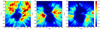 |
Fig. 1 Crosscuts along the planes XY, XZ, and YZ in the L19 3D dust extinction map. The Sun is at the center. The X axis points from the Sun to the Galactic center at Galactic longitude l = 0°, the Y axis points towards l = 90° and the Z axis points to the North Galactic pole. The Galactic center is to the right in the left and middle panels and back to the reader in the right panel. The color scale shows
|


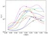 |
Fig. 2 Example of radial profiles of differential extinction ( |
2.2.2 Mathematical model for the inner surface of the LB shell
The inner surface of the LB shell can be visualized in 3D or in map format as shown in the top panel of Fig. 4. In order to characterize the geometrical shape of this surface, to extract its main features, and to provide a good model of it with a small number of parameters, we rely on a spherical harmonic expansion. By limiting the expansion to a maximum multipole degree, lmax, we can easily adjust the level of complexity of the modeled surface.
We utilize the Python version of the HEALPix package to handle spherical harmonics. For a given lmax, the routines return a set of positive spherical harmonic coefficients, from which we can build a model of the input surface smoothed out to the desired angular scale.
The expansion in spherical harmonics is meaningful to describe the shape of the inner surface of the LB shell. Indeed, the coefficients decay rapidly withincreasing l, which indicates that the spherical harmonic expansion converges for large lmax. We find that the power spectrum of the 2D map of rinner follows a power law with index − 2.95 up to l = 300.
It is clear that the modeling of the shell inner surface described above can be biased by the presence of small dust clouds inside the cavity. To correct for this bias, we proceed iteratively. We start from the 2D map of rinner extracted from the L19 3D dust extinction map in Sect. 2.2.1. Then for any chosen value of lmax, we proceed as follows:
- (i)
We expand the input map of the shell inner radius, rinner, in spherical harmonics up to lmax.
- (ii)
With theretained spherical harmonic terms, we approximate rinner by a modeled inner radius, rLB.
- (iii)
For all lines of sight with rLB > router, we reset rinner to rLB.
- (iv)
We repeat steps (i) to (iii) until the modeled surface does not change from the previous iteration.
The reason why step (iii) is needed is because the router value of a line of sight that points towards an intervening cloud is smaller than the rinner values of the neighboring lines of sight that avoid the intervening cloud. This iterative procedure should work as long as the intervening clouds are not too extended in the sky, such that statistically rLB is indeed determined by the inner surface of the LB shell. It is, however, clear that this procedure might mistakenly erase abrupt changes in rinner. This appears to happen for lmax = 2, 4, because the shape of the modeled inner surface is too simple compared to the input surface. For these values of lmax, we find that a total of 10 iterations is a good compromise that enables us to skip over intervening clouds, without artificially scooping out the shell inner surface. On the other hand, for lmax = 6, 8, 10, only 4, 8 and 10 iterations are required before the modeled inner surface becomes totally stable.
We visually check that the first and final models are very close to one another. Moreover, for each lmax, we quantify the difference between the first and final models by computing the mean Euclidean distance between the two sets of real-valued spherical harmonic coefficients, ãlm:
 (1)
(1)
where s and s′ refer to two different (here, the first and final) models of the shell inner surface. Real-valued spherical harmonics, which are better suited for describing real surface functions, are related to the standard complex spherical harmonic coefficients, alm, through
 (2)
(2)
Here, we normalize the alm coefficients to a00 because the overall scale of the LB shell is irrelevant for our magnetic field modeling in Sect. 3.
In Fig. 7, we plot the Euclidean distance between the first and final models of the shell inner surface, for several values of lmax (gray dotted line). We consider this distance as a measure of the intrinsic accuracy of our model of the shell inner surface based on a given 3D extinction map.
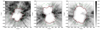 |
Fig. 3 Crosscuts along the planes XY, XZ, and YZ in the L19 3D dust extinction map, with the same conventions as in Fig. 1. The (common) gray scale shows
|


 |
Fig. 4 Full-sky map of (top) the inner surface of the LB shell (rinner) as extracted from the L19 3D extinction map (Sect. 2.2.1) and (bottom) our model of this surface through a spherical harmonic expansion up to lmax = 6 (Sect. 2.2.2). The maps are in Galactic coordinates, the center points towards the Galactic center and longitude increases to the left. |
2.3 Results
In the triptych of Fig. 3, we show our models of the inner surface of the LB shell as obtained through a spherical harmonic expansion up to different values of lmax (black lines). In the bottom panel of Fig. 4, we show a full-sky map of our model of the inner surface obtained for lmax = 6. The model can be directly compared to the input map shown in the top panel of the same figure.
2.4 Comparison with other 3D maps
In this subsection, we investigate the impact of the choice of the 3D extinction map on our modeling of the shape of the LB shell. It is important to test the stability of our results against other data sets. However, it is not our purpose to provide a comparison study between the different 3D maps of the dust density distribution that are available. Future analyses should help pinpoint which 3D map is the most reliable and which is the best suited for the kind of analysis presented here. The most advanced 3D maps that can compete with that of L19 are those from LE19, Green et al. (2019) and Chen et al. (2019).
Green et al. (2019) constructed a 3D map of dust reddening based on stellar parallaxes from Gaia DR2 and on stellar photometry from Pan-STARRS 1 and 2MASS. Their map relies on 800 million objects, has unprecedented angular resolution and extends out to a distance of several kpc, but it is limited by the Pan-STARRS footprint. It covers (only) about 75 percent of the sky for declination δ > −30°. Our model of the shape of the LB shell would suffer from this large hole in the sky, which would bias all the low lmax components.
Chen et al. (2019) used stellar parallaxes from Gaia DR2 together with optical and near-infrared photometry from Gaia, WISE and 2MASS to trace dust reddening. Because they focused on the Galactic disk, they analyzed only lines of sight with Galactic latitudes |b|≤ 10°. As a result, their map is not at all suited for our study.
In contrast, LE19 constructed a 3D map of dust reddening that is full-sky once projected on the sky, but covers a smaller volume than the L19 map, namely a (600 pc)3 cube centered on the Sun. Unlike L19, they constructed a statistical model with non-parametric kernel and applied a Bayesian variational scheme to Gaia DR2 distances and reddening estimates from Andrae et al. (2018), producing a set of fifty 3D maps. We refer the reader to their paper for further details on their inversion method and their results.
Focusing on the overlapping volume to compare with the 3D map of Lallement et al. (2018), LE19 showed that their mean reconstruction gives values of the dust density that range from a few orders of magnitude lower to one order of magnitude higher. The latter corresponds to a cloud size that is one order of magnitude smaller, which is expected given that Lallement et al. (2018) used a fixed minimum size for their two co-existent kernels. A comparison with the L19 map leads to the same conclusions, which again is expected since, despite the new hierarchical technique, the L19 final step also has a 25 pc resolution limitation. On the other hand, unexpectedly, the close vicinity of the Sun in the LE19 map appears to have too low reddening, that is, to be too empty, compared to other maps. As discussed in LE19, potential causes are the choice of the data sets used to reconstruct the 3D map, or an artifact of their reconstruction. In addition, the authors cautioned against using the external parts of their reconstructed map, as periodic boundary conditions were assumed for algorithmic reasons, and the northern and southern tops of the “chimneys” fall in this category (see below). Finally, the authors noted a pronounced tension in the 3D positions of some dust clouds. Despite the higher angular resolution of LE19, we find a good agreement in the sky positions of the clouds, but we also detect some differences in their distances to the Sun.
Our method can be directly applied to the LE19 maps since they are full-sky once projected onto the sky. Therefore, with the above caveats in mind, below we use the mean LE19 map to test the robustness of our model of the shape of the LB shell with respect to the adopted 3D extinction map. As performed in Sect. 2.2.1 with the L19 3D extinction map, we extract the radial profiles of differential extinction,  , smooth them using a Gaussian kernel with a standard deviation of 25 pc in order to eliminate spurious high-frequency variations in
  , and define the inner and outer surfaces of the LB shell.
In the triptych of Fig. 5, we show the modeled inner surface of the LB shell obtained in Sect. 2.2.2 with the L19 map, but over-plotted on the gray-scale dust density distribution with corresponding inner and outer surfaces of the LB shell from the LE19 map. An overall qualitative agreement is reached, but significant differences are observed. Additional structures, likely to be intervening clouds, appear in the LE19 map or are found to be closer to the Sun than in the L19 map. For some lines of sight, the opposite trend is observed, as illustrated in the right panel of Fig. 5. In fact, in the LE19 map, the inner surface is often found far from the Sun and quite close to the boundary of the modeled interstellar volume. In this region of space, we expect the distance to the shell to be biased in a non-trivial way by the presence of the boundary. LE19 did indeed caution against the fact that the periodic boundary conditions used in their inversion process might produce artifacts up to about 15 pc from the sides of the modeled volume. We estimate that these hardly quantifiable systematics are propagated further inside the volume, for example, up to about 50 pc, by the line-of-sight smoothing that we adopt to eliminate spurious noise in the differential extinction radial profiles.
To go beyond the qualitative comparison given around Fig. 5, we model the inner surface of the LB shell based on the LE19 3D map in the same manner as we model it in Sect. 2.2.2 based on the L19 map. The results are displayed in the triptych of Fig. 6. We also compute the Euclidean distances (Eq. (1)) between the real-valued spherical harmonic coefficients of the modeled inner surfaces derived from the L19 and LE19 maps, for several values of lmax. These distances are plotted in Fig. 7. They are about one order of magnitude larger than the distances between the first andlast iterations in our modeling procedure (see Sect. 2.2.2).
In conclusion, it appears that our models of the inner surface of the LB shell depend quite substantially on the underlying 3D extinction map. In view of the above discussion, we prefer to rely on the L19 map; we consider the resulting models of the shell inner surface to be more suitable for our present purpose.
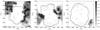 |
Fig. 5 Same as for Fig. 3, except that the underlying dust density distribution and the corresponding inner and outer surfaces of the LB shell (red and green lines, respectively) are from the LE19 3D map. Our models of the inner surface (black dotted, dashed and solid lines) are still based on the L19 map. |
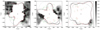 |
Fig. 6 Same as for Fig. 5, except that our models of the inner surface of the LB shell (black dotted, dashed and solid lines) are now based on the LE19 map. |
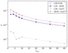 |
Fig. 7 Euclidean distances (d, given by Eq. (1)) between several models of the LB shell inner surface as a function of the maximum multipole degree (lmax). The gray dotted line compares the first and final iterations of the iterative procedure discussed in Sect. 2.2.2 and applied to the L19 data. The blue dashed line compares the final models obtained with the L19 and LE19 data. The orange and purple dot-dashed lines compare the final models obtained with the L19 and LE19 data, respectively, with the shape of the LHB from Liu et al. (2017) (see Sect. 2.5). |
2.5 Comparison with the shape of the Local Hot Bubble
Based on data from the DXL sounding rocket mission, Liu et al. (2017) obtained a reliable map of the X-ray emission attributed to the LHB.Their modeling of the X-ray emission allowed them to estimate the shape of the LHB, among other physical parameters, under the assumption of hot gas homogeneity. The shape of the LHB was found to match qualitatively well the shape of the dust cavity in the 3D extinction map of Lallement et al. (2014).
Comparing X-ray data, which probe the hot ionized gas, with extinction data, which probe the dust, is a milestone in its own right towards a global understanding and physical modeling of the multi-phase ISM, in particular in the solar vicinity. A detailed comparison between the physical properties inferred from both kinds of data is beyond the scope of our paper. In this subsection, we are content to compare the shape of the X-ray emitting LHB with the shape of the shell inner surface that we modeled from dust extinction maps. To do so, we compute the Euclidean distances (Eq. (1)) between the real-valued spherical harmonic coefficients of both shapes, for several values of lmax.
For the reasons explained below Eq. (2), we use the normalized coefficients. This enables us to get rid of an overall scale difference between the LHB and the shell inner surface. We note that only the shell, which is seen through dust extinction, has a reliable size; the LHB has an uncertain size that depends on the assumed electron density. The computed distances are plotted in Fig. 7, which indicates that the shapes of the LB derived from different tracers compare as well as the shapes extracted from different extinction maps. This suggests an overall consistency across the different phases of the ISM.
3 Modeling the magnetic field in the LB shell
A18 presented the first physical model of the magnetic field in the shell of the LB. Their model relies on the common assumption that the LB was created by supernova explosions, which swept out a cavity of hot ionized gas and pushed most of the evacuated matter, together with the frozen-in magnetic field, into a dense shell of cold neutral gas and dust around the cavity. Their model further assumes that the initial magnetic field is uniform in strength and direction within the whole volume encompassed by the present-day LB, that the expansion motions driven by the explosions are purely radial, and that the shell is very thin (in the sense that it can be approximated by a 2D surface). Adopting a spheroid to describe the shape of the shell, A18 constrained their magnetic field model by fitting it to the 2015 Planck 353 GHz observations of the dust polarized emission towards the Galactic polar caps.
In this second part of the paper, we go one step further than what was done by A18: we take up their magnetic field model, relax their simplifying assumption of a spheroidal shell, and adopt instead the more realistic geometry derived in Sect. 2 on purely observational grounds. To remain consistent with the very thin shell approximation, we replace the actual thick shell found in Sect. 2 (see, e.g., Fig. 3) by an idealized very thin shell. A priori the best way of defining this very thin shell would be to identify it with the surface of maximum density inside the actual thick shell, that is, the surface at rmax where the differential extinction,  , reaches its first maximum beyond rinner. In practice, however, this criterion does not work, because some lines of sight turn out to have rmax > router (see, e.g., cyan radial profile in Fig. 2). Moreover, as already discussed in Sect. 2.2.1, router is often unreliable. Since neither router nor rmax can be confidently determined in all directions, we take the inner surface of the actual thick shell to represent the very thin shell. We note, however, that the outer surface appears to have a shape roughly similar to that of the inner surface. Since our fit to the polarization data depends only on the shape of the shell, not on its size, the impact of substituting the inner surface of the shell for the shell itself is probably small. In the remainder of this section, the word “shell” refers to the idealized very thin shell.
3.1 Magnetic field model
We start with the general magnetic field model derived in A18. The present-day (ordered) magnetic field in the LB shell, B, can be fully described in terms of the initial magnetic field, B0, the shape of the shell, and the position of the explosion center. If several explosions took place, the explosion center is taken to be a point from which the expansion motions driven by the explosions can be considered to be purely radial. In a spherical coordinate frame centered at the explosion center, the mathematical expression of B as a function of position r is given by Eq. (6) in A18:
![Mathematical equation: \begin{equation*} \mathbf{B}(\vec{r}) = \frac{r_0}{r}\, \frac{\partial r_0}{\partial r}\, \frac{1}{\vec{n} \cdot \vec{e}_{\textrm{r}}} \left[ \vec{n} \times (\mathbf{B}_0 \times \vec{e}_{\textrm{r}}) \right],\end{equation*}](/articles/aa/full_html/2020/04/aa37157-19/aa37157-19-eq12.png) (3)
(3)
where n is the unit vector normal to the surface of the shell, er is the unit vector in the radial direction (from the explosion center), and r0 is the initial radial position of a particle presently at radial position r.
The measured polarized intensity of the thermal dust emission depends on the orientation of the magnetic field, but not on its strength. Therefore, the prefactor in Eq. (3) is irrelevant and only the orientation of the vector within square brackets matters. In the expression of this vector, the unit vector normal to the shell, n, can be derived directly from the known shape of the shell; the radial unit vector, er, is set by the position of the explosion center, which, in turn, is defined by its Cartesian coordinates (δx, δy, δz); and the orientation of the initial magnetic field, B0, is given by its Galactic angular coordinates, (l0, b0). Hence, we are left with a total of five free parameters: (δx, δy, δz, l0, b0).
For the shape of the LB shell, we adopt the inner surface extracted from the L19 3D extinction map (in Sect. 2.2.1) and expanded in spherical harmonics up to lmax (in Sect. 2.2.2). We only consider values of lmax ≤ 10. Larger values of lmax would enable us to capture finer details of the original shell surface, but because of the low resolution of the L19 3D extinction map, these fine details are probably not physical. More important, our simple magnetic field model is not suited for a very convoluted shell. It is, therefore, legitimate to restrict our investigation to smooth shell models.
It directly emerges from Eq. (3) that for a given shell surface, that is, for given normal vector, n, and for a given orientation of the initial magnetic field, B0, the orientation of the present-day magnetic field, B, remains unchanged when the explosion center is displaced along a line parallel to B0. It then follows that there will be a degeneracy between the three coordinates of the explosion center, with the degeneracy line being parallel to B0. In other words, our modeling will not enable us to determine the 3D location of the explosion center, but only to constrain its 2D position in a plane perpendicular to B0.
3.2 Constraints from dust polarized emission
To constrain the free parameters of our magnetic field model, we compute the associated Stokes parameters Q and U of the linearly polarized thermal dust emission, and we confront them to the observed Stokes parameters at 353 GHz from the 2018 Planck data release (hereafter PR3).
We start from the integral equations for the Stokes parameters similar to those given in Appendix B of Planck Collaboration Int. XX (2015)2. For optically thin emission at frequency ν:
![Mathematical equation: \begin{equation*}I=\int S_{\nu}\,\left[1-\mathfrak{p}_0\left(\cos^2\gamma-\frac{2}{3}\right)\right]\, n_{\mathrm{H}} \, \sigma_{\mathrm{H}} \, \mathrm{d} s, \end{equation*}](/articles/aa/full_html/2020/04/aa37157-19/aa37157-19-eq13.png) (4)
(4)
 (5)
(5)
 (6)
(6)
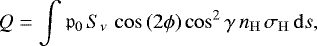
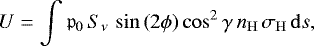
where the integrals are computed along the line of sight over the emitting region (here, the LB shell); Sν is the source function, 𝔭0 a parameter related to dust polarization properties combining grain cross sections and the degree of alignment with the magnetic field, nH the gas density, σH the dust cross-section per hydrogen atom averaged over angles, γ the angle of the local magnetic field to the plane of the sky, and ϕ the local polarization angle (see Fig. 14 in Planck Collaboration Int. XX 2015).
As in Lee & Draine (1985) and Planck Collaboration Int XLIV (2016), we account for variations in the magnetic field orientation along the line of sight by introducing an effective depolarization factor F that includes turbulence effects as well as small departures of our ideal model from reality. Within this approximation, the Stokes parameters Q and U may be written as:
 (7)
(7)
where p0 = F 𝔭0 is an effective polarization fraction, Bθ and Bϕ are the plane-of-sky components of the ordered magnetic field expressed in the spherical coordinate system centered on the observer (eθ points southwards and eϕ eastwards). Equations (7) introduce the sky map Id defined as
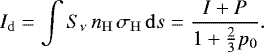 (8)
(8)
Following Planck Collaboration Int XLIV (2016) and Vansyngel et al. (2017), we approximate Id with I. We note that the mean values of Id and I are equal when averaging over angles. Hereafter, we assume that p0 is constant across the fitted sky region. This assumption is supported by the tight scaling observed between the amplitude of the dust polarization power spectra and the dust total intensity, with no systematic difference between the northern and southern Galactic latitudes (Planck Collaboration Int. XXX 2016; Planck Collaboration XI 2020).
In principle, the model of the magnetic field in the LB shell and its contribution to the dust polarized sky can be evaluated for the full-sky, corresponding to a first layer of the Galactic dust polarized foregrounds. However, because our model does not include any component from the large-scale Galactic magnetic field, we follow A18 in restricting the fitted area to the Galactic polar caps, |b| ≥ 60°. Using star optical polarization measurements and star distances to estimate the line-of-sight distance of the region responsible for the 353 GHz polarized emission, Skalidis & Pelgrims (2019) provided statistical evidence that in the Galactic polar caps the 353 GHz polarized emission is dominated by a dusty and magnetized structure extending from about 200 to 300 pc from the Sun. We naturally identify this structure with the LB shell, as also suggested by the triptych of Fig. 3.
We constrain the free parameters of our magnetic field model by maximizing the profiled log-likelihood function,
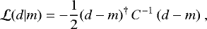 (9)
(9)
where d is the concatenation of the observed Stokes Q and U maps and m is the concatenation of the modeled Q and U maps.
The observed Stokes Q and U maps are based on products from the third Planck data release that we downloaded from the Planck Legacy Archive3. For our Galactic study, we consider the Q and U 353 GHz maps made from the polarization-sensitive bolometers only, as recommended in Planck Collaboration III (2020) and in Planck Collaboration XII (2020). We smooth them to a resolution of 80′.
The modeled Q and U maps are computed from Eq. (7) and adjusted to the observations through a linear fit that accounts for the pixel uncertainties4. The different parameters entering Eq. (7) are obtained as follows: the last factor, which depends only on the normalized (ordered) magnetic field vector in the shell, is directly taken from our magnetic field model described in Sect. 3.1. The factor Id is approximated by the dust total intensity, I, and for I we use the map that results from the GNILC component separation algorithm (Remazeilles et al. 2011). Following the recommendation from Planck Collaboration XII (2020, see their Sect. 2), we subtract from this intensity map the contribution from the cosmic infrared background monopole (452 μKCMB) and add back a fiducial Galactic offset (63 μKCMB). This map has a uniform resolution of 80′. Finally, the effective polarization fraction, p0, is a scaling factor computed from a linear fit for each set of free-parameter values. As in Pelgrims et al. (2018), this choice allows for the optimization of the computation time and reduces by one the number of free parameters of the model.
We downgrade the observed maps of Q, U, and I to the HEALPix grid of Nside = 128 and convert them to MJy sr−1 using the unit conversion factor of 287.5 MJy sr−1 K given in Planck Collaboration III (2020). The resulting Q and U maps used as observational reference for our fits are shown in the top row of Fig. 8.
The covariance matrix C entering Eq. (9), assumed diagonal, takes into account the noise in the Planck Q and U data ( ) and a contribution from the turbulent magnetic field component (
 ) that is otherwise not accounted for in the model and which is added in quadrature. As in A18, the latter is estimated using modeled Q and U maps from Vansyngel et al. (2017), which fit the Planck dust power spectra at 353 GHz. The dispersion of Q∕I and U∕I in these maps, measured over the northern and southern Galactic polar caps separately, yields
 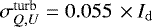 . We note that this estimate is based on a model where the ordered magnetic field is assumed to have a uniform orientation. The corresponding value for the more elaborate model derived in this work could be smaller. For the statistical noise, we use the covariance matrix of the Q and U GNILC maps, which are already delivered at 80′ resolution. We convert them using the conversion factors reported in Table B.1. of Planck Collaboration XII (2020) so that they correspond to the polarization-sensitive bolometers Stokes maps.
3.3 MCMC fit
When modeling complex data, Markov chain Monte Carlo (MCMC) methods have the strong advantage that they provide direct insight into the correlations and degeneracies between the different model parameters. They also make it possible to fully explore the parameter space and to monitor the exploration up to completion.
In order to explore the parameter space, find the best-fit values of the parameters and sample their posterior distributions, we use the emcee MCMC Python software written by Foreman-Mackey et al. (2013), who implemented the Affine-Invariant sampler proposed byGoodman & Weare (2010). Considering a non-informative prior, we require that the explosion center be located within the present-day LB cavity, namely, within the volume interior to our modeled LB shell. We emphasize that this common-sense requirement remains consistent with the conclusion of Maíz-Apellániz (2001) that the supernovae contributing to the LB over the past 10 Myr exploded just outside the boundary of the present cavity; indeed, the LB and its surrounding ISM probably drifted as a whole with respect to the Local Standard of Rest (by ≃ 150 pc in 10 Myr; see Sect. 1) and this drift may easily have brought the LB entirely past the explosion sites. With our simplifying assumption of a single explosion center, the LB drift can simply be seen as a translation of the coordinate reference frame. We also note that the above prior sets limits on the location of the explosion center in the direction of the initial magnetic field, which otherwise is not constrained at all by our fit to the Planck data (see discussion at the end of Sect. 3.1).
To optimize the exploration of the parameter space, we proceed in two stages. In the first stage, we identify the region of parameter space that maximizes the log-likelihood. In the second stage, we determine the set of best-fit parameter values and properly sample the posterior distributions. Thus, in the first stage, 500 Markov chains are initialized with uniform distributions over a restricted parameter space defined as:
-
{δx, δy, δz}∈ [−70, 70] pc
-
![Mathematical equation: $b_0 \in [-90,\,90]^{\circ}$](/articles/aa/full_html/2020/04/aa37157-19/aa37157-19-eq23.png) &
& ![Mathematical equation: $l_0 \in [0,\,180]^{\circ}$](/articles/aa/full_html/2020/04/aa37157-19/aa37157-19-eq24.png) ,
,
and the MCMCalgorithm is run for 1000 steps. This first stage can be considered as a burn-in phase of the MCMC experiment. In the second stage, we retain the best 250 chains obtained at the last MCMC step of the first stage; these chains are initialized at their last positions in parameter space, and the MCMC algorithm is run until the convergence criteria proposed by Gelman & Rubin (1992) are fulfilled for all the model parameters, with a threshold value of 1.03. We test for convergence every 100 MCMC steps. For all the fits presented in this paper, convergence is reached within 5000 steps. We verified on one of the fits that the same result is obtained when initializing ten times more Markov chains at the first stage within a wider volume of parameter space.
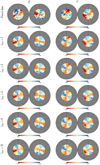 |
Fig. 8 Orthographic views of the Q (left) and U (right) maps at 353 GHz. From top to bottom: Planck PR3 data and best-fit maps corresponding to the modeled shapes of the LB shell obtained from the L19 3D extinction map, with lmax = 2, 4, 6, 8, and 10. The background structures underlying the maps come from the dust column density taken from the data. Units are MJy sr−1. In orthographic views, the North and South Galactic Poles lie at the center of the left and right circles, respectively, the vertical solid radius shows longitude 0°, and the left and right panels touch at l = 90°. The gray area corresponds to the region |b| < 60°, which is notconsidered in the fitting procedure. |
3.4 Results
We use our MCMC procedure to fit the Planck Q and U maps and thereby constrain the five free parameters of our magnetic field model. We consider the cases when the spherical harmonic expansion of the inner surface of the LB shell in Sect. 2.2.2 is truncated at lmax = 2, 4, 6, 8, and 10. We present the results of the fits in Sect. 3.4.1 and discuss systematic uncertainties in Sect. 3.4.2.
Since dust polarization only gives the orientation of the magnetic field, not its direction, each solution for (l0, b0) actually corresponds to the pair of solutions (l0, b0) and (l0 + 180°, − b0). Among these two solutions, we select the one that is closer to the large-scale magnetic field direction derived from rotation measures of nearby pulsars, which is almost equivalent to selecting the value of l0 that lies in the range [0°, 180°] (e.g., Ferrière 2015).
3.4.1 Magnetic field model
The best-fit Q and U maps obtained with the five values of lmax are shown in Fig. 8, below the observed Planck maps. For the purposes of visualization, Fig. 9 displays the 1D and 2D marginalized posterior distributions of the fits obtained with lmax = 2, 6, and 10. The posterior distributions are produced from converged fractions of the MCMC chains.
In these corner plots, it appears that the coordinates of the explosion center, (δx, δy, δz), and those of the initial magnetic field direction, (l0, b0), are not correlated around the best-fit values. Similar results are obtained with lmax = 4 and 8. The 2D marginalized posterior distributions of (δx, δy, δz) reflect the model degeneracy discussed at the end of Sect. 3.1: the orientation of the present-day magnetic field in the shell is insensitive to the position of the explosion center along the direction of the initial magnetic field, B0.
Table 1 lists the best-fit values of the five model parameters. The quoted uncertainties correspond to the standard deviation of the 1D marginalized posterior distribution of each parameter. They only account for the data noise and the turbulent component of the magnetic field.
Using the 2015 Planck data release, A18 found that the dominant contribution to the uncertainty budget on their model parameters is from the Planck residual systematics. Here, to provide a full error budget, we need to assess the impact on our model results of both residual systematics in the Planck data and uncertainties in the 3D extinction map.
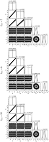 |
Fig. 9 1D and 2D marginalized posterior distributions of the model free parameters. The modeled shapes of the LB shell are obtained from the L19 3D extinction map, with lmax = 2, 6, and 10. The verticaldashed lines show the 2.5, 50 and 97.5 percentiles. |
Best-fit parameter values of the adjusted magnetic field model for the values of lmax used to model the shape of the LB shell based on the L19 3D extinction map.
Best-fit parameter values and corresponding results of the E2E simulations, for the modeled shapes of the LB shell obtained from the L19 (top) and LE19 (bottom) 3D extinction maps, with lmax = 6.
3.4.2 Systematic uncertainties
In this section, we assess the uncertainties associated with first the Planck data systematics and second the 3D extinction map used to compute the inner surface of the LB shell (see also Sect. 2.4).
For the Planck residual systematics, we follow the following three steps. First, we produce mock Q and U maps based on the model maps computed for the best-fit parameters, to which we add independent realizations of the Planck systematics. Here, we use the end-to-end (E2E) simulations available in the Planck Legacy Archive (see Appendices A.1 and A.2 in Planck Collaboration XI 2020)5. Next, we fit each set of Q and U mock maps with our MCMC code in the same way as we fitted the Planck maps, using the same covariance matrix and Id map. Last, we compare the best-fit parameter values obtained for 10 mock samples with the input model values to quantify the uncertainties associated with the Planck residual systematics. To estimate the uncertainties associated with the 3D extinction map, we repeat the analysis of the mock maps and the fit to the Planck maps, using the LB shape derived from the LE19 map instead of the L19 map.
Table 2 summarizes the results of this data analysis. For each of the 3D extinction maps, we first report the best-fit parameter values and the standard deviations of the 1D marginalized posterior distributions obtained by fitting to the Planck data. In the second line, we report the mean values and the standard deviations of the best fits to the 10 mock maps. Here are the conclusions we draw from this analysis.
- (i)
The Planck residual systematics do not induce bias in the best-fit parameter values since the input parameter values are always found within one standard deviation from the mean values measured in the mock maps.
- (ii)
The difference between input and output parameter values is slightly larger than the uncertainties from the fit to the Planck data, which showsthat the residual systematics are a significant source of uncertainty. This conclusion is substantiated by the dispersions in the best-fit values of l0 and b0, which are larger than those derived in the MCMC data fit for the Planck noise and turbulence. We note that, as expected, the uncertainties in l0 and b0 are smaller for the PR3 maps than those obtained in A18 for the previous version of the Planck maps.
- (iii)
The best-fit parameter values depend significantly on the 3D dust maps used to model the geometry of the LB shell. Indeed, for most of the model parameters, the posterior distributions obtained with the LE19 map are significantly different from the corresponding distributions obtained with the L19 map. At this stage, we recommend that both solutions be considered, as neither one is actually better than the other (however, see the discussion in Sects. 2.4 and 3.5.4). The dispersion between the different models is more representative of the margins of error.
3.5 Discussion
This work extends the analytical modeling of the local Galactic magnetic field in A18 into a consistent model where the shape of the LB shell is derived from a 3D extinction map (L19 or LE19), rather than approximated with an ad-hoc geometry. To assess and discuss the validity of our model, we compare it to two other models that we fitted to the same Planck PR3 353 GHz data and with the same MCMC code. One of these models is the spheroid model of A18, the other one assumes, as in Planck Collaboration Int XLIV (2016), that the magnetic field orientation is uniform over each Galactic polar cap. In all cases, the models were fitted over both polar caps with a single value of p0. As a basis for the model comparison (discussed below), Table 3 provides a few representative quantities corresponding to the best fit of each model.
Comparison of the best-fit magnetic fields for four different models discussed in the text.
3.5.1 Goodness of fit
Our model fits the data with good reduced χ2. The values of  in Table 1 increase with increasing lmax, from
  for lmax = 2 to
  for lmax = 10. The variation is small but systematic. This trend suggests that the increasingly detailed structure of the LB surface that the model captures as lmax increases does not match structure in the Planck polarization maps. Our models appear to be mainly successful at modeling the magnetic field orientation in the LB shell on very large angular scales, that is, the first few multipoles accounting for the variation from the northern and southern polar caps.
This conclusion is supported by the comparison with the reduced χ2 obtained when fitting either a model with uniform magnetic field orientation over each polar cap ( ) or the spheroid model of A18 (
 ) to the same Planck PR3 data. It is interesting to note that the reduced χ2 is only slightly smaller for the A18 spheroid model (
 ) than for our model with lmax = 2 (
 ), even thoughour model has three fewer free parameters. This is quite satisfying, especially as the best-fit spheroid obtained by A18 poorly matches the LB shape derived from extinction and X-ray data.
For lmax = 6, the reduced χ2 is smaller when the LB shell is modeled using the LE19 3D extinction map (χ2 = 0.61) than using the L19 map (χ2 = 0.75). This indicates that the former is somewhat favored by the fit of our magnetic field model to the Planck data. However, this conclusion has to be confronted to the caveats drawn in Sect. 2.4 regarding the use of the LE19 map to model the shape of the LB shell (see also our discussion in Sect. 3.5.4).
The values of the reduced χ2 obtained for the three tested models of the magnetic field in the solar neighborhood are all below unity. This suggests an overestimation of the uncertainties entering the log-likelihood that we are maximizing. It is the contribution from the turbulent component of the magnetic field ( ) that dominates the uncertainty budget. It is, therefore, likely that the degree of turbulence that we adopt for our magnetic field modeling, and which we take from Vansyngel et al. (2017), is globally overestimated. This does not impact the results of our fit, which depend only on the relative weighting of pixels, not on the actual value of the uncertainties.
3.5.2 Model parameters
Here, we discuss the best-fit values obtained for our free parameters, namely, the angular coordinates (l0, b0) of the initial magnetic field, B0, and the Cartesian coordinates (δx, δy, δz) of the explosion center.
The best-fit values of l0 are all ~ 70°: the values obtained from the L19 map (for different values of lmax; see Table 1) lie in the range ≃ 72°–73°, while the value obtained from the LE19 map (for lmax = 6; see Table 2) is ≃68°. These values correspond to a magnetic pitch angle ~20° in the solar neighborhood (≃17°−18° from the L19 map and ≃22° from the LE19 map). This pitch angle is consistent, within the error bars, both with the A18 value and with the values obtained by Pelgrims & Macías-Pérez (2018) upon fitting large-scale Galactic magnetic field models to full-sky Planck dust polarized emission maps.
The best-fit values of b0 appear to be much more sensitive to the chosen value of lmax and to the adopted 3D extinction map: the values obtained from the L19 map lie in the range ≃ 13°−17°, while the value obtained from the LE19 map is ≃3°. These values indicate that the magnetic field in the solar neighborhood points upwards, crossing the Galactic plane at a small angle. For comparison, the spheroid model of A18 fitted to the Planck PR2 353 GHz data predicts a magnetic field pointing downwards, with an angle to the Galactic plane ≃ − 16°. However, when re-fitting the spheroid model of A18 to the Planck PR3 353 GHz data, we find b0 ≃−2°, which is almost half-way between the value reported in A18 and the values obtained here from the L19 map. Hence, part of the discrepancy between A18 and the present study can be attributed to the different data sets (PR2 versus PR3).
The best-fit position of the explosion center depends quite sensitively on the chosen value of lmax and on the adopted 3D extinction map. Moreover, the error bars are always large, especially in the Y -direction. This is because the position of the explosion center cannot be constrained in the direction of the initial magnetic field, B0 (see end of Sect. 3.1), except for the requirement that it be contained within the present-day cavity. Since B0 is found to be nearly parallel to the Galactic plane (b0 close to 0°) and at a small angle to the Y -direction (l0 close to 90°), δy is very poorly determined, with error bars comparable to the LB radius in the Y -direction. The error bars on δz are smaller, with the result that none of the best-fit positions is found close to the Galactic plane (δz = 0). Only the solution obtained from the L19 map, with lmax = 6, is compatible with |δz| ≲ 50 pc within the uncertainties.
3.5.3 Mean orientation of B and effective polarization fraction p0
We compute the mean magnetic field direction for our best-fit models by averaging the Cartesian coordinates of B over each Galactic polar cap. For the shape of the LB shell obtained from the L19 3D extinction map, with lmax = 6, we find that the mean magnetic field points towards Galactic coordinates (l, b) = (71° ± 1.3°, −10.9° ± 0.1°) and (74° ± 1.4°, 5.8° ± 0.7°) in the northern and southern polar caps, respectively. The corresponding coordinates of the mean magnetic field obtained with the LE19 map, still with lmax = 6, are (l, b) = (72.5° ± 0.6°, −0.1° ± 1.9°) and (76.8° ± 1.4°, −15.2° ± 2.5°) in the northern and southern polar caps, respectively. The error bars are derived from the results obtained on the mock observations described in Sect. 3.4.2. The mean magnetic field coordinates do not depend much on lmax. However, they depend significantly on the adopted geometric model (see Table 3).
The mean dust polarization fraction over the Galactic polar caps involves the product of the effective polarization fraction, p0, and the mean value  , where γ is the angle between B and the plane of the sky. Thus, in the fit to the data, the value of p0 depends on
  . In our best-fit model based on the L19 extinction map, with lmax = 6, the value averaged over both polar caps is
  , with a small scatter, which implies that the mean magnetic field has a small angle to the plane of the sky (γ ≈ 15°). For comparison, in the best-fit model based on the LE19 extinction map, still with lmax = 6, and in the “uniform” and A18 spheroid models applied to the Planck PR3 data,
  , 0.79, and 0.66, respectively, which means that the mean magnetic field is more significantly tilted to the plane of the sky (γ ≈ 32°, 27°, and 36°, respectively). These differences in the averaged value of
  explain the differences in the value of p0. It is interesting to note that the product
  is roughly conserved between the different models listed in Table 3.
3.5.4 Comparison with radio polarization data
The analysis of the Parkes survey of the southern sky (δ < 20°) at frequencies of 300–480 MHz (Wolleben et al. 2019) presented by Dickey et al. (2019) provides an additional constraint, which may be used to discriminate between the different models listed in Table 3. The intensity-weighted mean of the Faraday depth  , has average values
  rad m−2 and
  rad m−2 over the northern and southern polar caps, respectively, with an uncertainty ~ 0.3 rad m−2 (see Fig. 8 in Dickey et al. 2019). We note that these values have the same signs as the corresponding rotation measures (RMS),
  rad m−2 and
  rad m−2 (see Fig. 11 in Dickey et al. 2019), measured in the map of Galactic RMs built from observations of extragalactic sources by Oppermann et al. (2015). The positive signs of the two sets of values indicate that the line-of-sight magnetic field points towards us from both the North and South Galactic poles. This is in agreement with the results obtained here from the L19 map, since we find that the magnetic field points towards negative latitudes for the northern polar cap (bN < 0°) and to positive latitudes for the southern cap (bS > 0°). The positivesigns of
  and
and  are also in agreement with the predictions of the “uniform” model, whereas they are in opposition to the signs predicted by both the A18 spheroid model and the shell model based on the LE19 map.
Within the simple model presented by Sokoloff et al. (1998), the mean Faraday depth, towards either polar cap is given by  , where K = 0.81 rad m−2 cm3 μG−1 pc−1, DM is the dispersion measure, and BZ is the magnetic field component along the Z-axis perpendicular to the Galactic plane. This is an approximative model, which we use for qualitative comparison. For example, the ratio between the full RM through the Galaxy and the mean Faraday depth is 2 in the model, while the observed ratio is ~ 4. From pulsar measurements, we know that DM ≃ 26 pc cm−3 (Gaensler et al. 2008), and thus
  (rad m−2)| ≃ 10.5 |BZ(μG)|. To match the observed values of
  and
and  , |BZ | must be ~ 0.15 μG, that is, a small fraction of the total strength (a few μG, Beck et al. 2003) of the mean magnetic field in the solar neighborhood. In other words, the magnetic field in each polar cap must be nearly in the plane of the sky, that is, the angle γ must be small. This, too, is in agreement with the results obtained from the L19 map, which lead to values of
  and
and  close to 1. The agreement is not as good with the predictions of the other models listed in Table 3, which give smaller values of
  and
and  . Altogether, our comparison with the mean Faraday depths derived by Dickey et al. (2019) leads us to give preference to the shell model based on the L19 map.
4 Summary and perspective
In this paper, we pursued a physically motivated approach to model interstellar polarization data at high Galactic latitudes in a self-consistent way, which involved modeling the magnetic field in that part of the sky. We relied on observational evidence showing that the dust polarized emission is dominated by a nearby dusty and magnetized structure. Associating this structure with the shell of the Local Bubble (LB) led us to model the magnetic field in the LB shell, for which polarization data can be obtained. We used a dedicated analytical model that relates the structure of the magnetic field in the LB shell to the shell geometry and we extracted the latter from actual 3D maps of the local dusty ISM.
This work is, therefore, two-fold. First, we extracted and modeled the geometry of the LB shell. Second, we inserted the resulting shell model into our analytical model of the magnetic field in the shell, which we then fitted to the Planck PR3 353 GHz polarization data at high Galactic latitudes. The key steps of this process and the main results are summarized below.
The first part of the paper focuses on the shape of the LB shell. We first we developed an ad-hoc method to extract the LB shell from 3D extinction maps through the identification of its inner and outer surfaces. We applied this method to the most recent 3D extinction maps that cover the full sky, namely, the maps from Lallement et al. (2019, hereafter L19) and from Leike & Enßlin (2019, hereafter LE19). We then expanded the shell inner surface in spherical harmonics, up to a variable maximum multipole degree, lmax, which enabled us to model its shape with the desired level of complexity. We compared the results obtained from the two extinction maps both with each other and with the shape of the Local Hot Bubble derived by Liu et al. (2017) from X-ray emission data. Both comparisons indicated overall agreement, with, however, noticeable differences in the details. The overall agreement between the LB shapes inferred from extinction maps and from X-ray emission data lends credence to our multi-phase view of the LB. We hope that our modeling of the dusty LB and the agreement found with the Local Hot Bubble will motivate further investigations and will help understand and physically model the multi-phase ISM in the solar vicinity.
The second part of the paper focuses on the magnetic field in the LB shell. Following up on the work of Alves et al. (2018, hereafter A18), we used the shape of the shell inner surface derived in the first part of the paper as input to the A18 analytical model of the magnetic field in the LB shell. Fixing the shape of the shell inner surface left us with only five free parameters: the three Cartesian coordinates of the explosion center and the two angular coordinates of the initial magnetic field. Using a MCMC method, we fitted our magnetic field model to the dust polarized emission at high Galactic latitudes (|b| > 60°) as measured by Planck. The fit was performed for different values of lmax.
Our model fits the Planck data with good reduced χ2, close to the value obtained for the spheroid model of A18, which however has three more free parameters. Moreover, the best-fit spheroid of A18 does not match the observed geometry of the LB, whereas our modeled shell, which is directly derived from 3D extinction data, automatically does.
The derived orientation of the initial magnetic field, B0, appears to be stable for the different models of the shell inner surface that we tested (models with different values of lmax) or different underlying extinction maps). It is also consistent with models of the large-scale Galactic magnetic field. However, our models of the present-day magnetic field in the shell show more complexity in their geometry than those large-scale Galactic magnetic field models, including a North-South asymmetry. The position of the explosion center is only constrained in a plane perpendicular to B0, and even there it is only loosely constrained. None of the best-fit positions are found within less than ~ 100 pc from the Galactic plane. It is unclear whether this is clashes with existing models of the origin of the LB.
For the shell model derived from the L19 extinction map, the mean magnetic field in each polar cap has a small angle to the plane of the sky, and (assuming l0 ∈ [0°, 180°]) its line-of-sight component points towards us. Both results are in agreement with Faraday spectra of the Galactic diffuse synchrotron emission from the nearby ISM. The corresponding results obtained for either the shell model derived from the LE19 map, the “uniform” model, or the A18 spheroid model (see Table 3) do not show the same agreement with the Faraday spectra. It is, therefore, the LB shell model based on the L19 map that we consider to be the best.
We further investigated the sources of uncertainty in our approach to model the dust polarized emission in the Galactic polar caps. We considered the impact on our fits of the Planck residual systematics at 353 GHz and of the choice of the 3D extinction map used to extract and model the shape of the LB shell. We found that the largest uncertainty in our modeling came from the choice of the 3D extinction map, which, at this stage, was found to strongly depend on the underlying data set. Significant improvements are expected in that research area.
In principle, the modeling of the magnetic field in the LB shell and its contribution to the dust polarized sky can be evaluated for the full sky, corresponding to a first layer of the Galactic dust polarized foregrounds. In future studies, we will extend our modeling towards lower Galactic latitudes, where it will be required to connect the local magnetic field to the large-scale Galactic magnetic field. In a way, with this paper, we are setting the stage for the next generation of Galactic magnetic field models which would integrate external data sets or specific models derived from them. As a consequence, we expect this paper and our results to be useful both for modeling the local ISM as traced by its different components and modeling the Galactic dust polarized emission, a long-awaited input for studies of the polarized foregrounds to the CMB and to the optical polarization of extragalactic sources (Pelgrims 2019).
Acknowledgements
We would like to warmly thank Marta Alves for all the inspiring discussions and motivations that took place during the early phases of this project. We thank Kostas Tassis for comments that help improving the presentation of the work. We also thank J. van Loon for his fruitful review. This work has received funding from the European Research Council (ERC) under the European Unions Horizon 2020 research and innovation programme under grant agreement No. 771282, and by the Agence Nationale de la Recherche (project BxB: ANR-17-CE31-0022). We acknowledge the use of data from the Planck/ESA mission, downloaded from the Planck Legacy Archive, and of the Legacy Archive for Microwave Background Data Analysis (LAMBDA). Support for LAMBDA is provided by the NASA Office of Space Science. Some of the results in this paper have been derived using the HEALPix (Górski et al. 2005) package.
Appendix A Supplementary material
In Fig. A.1 we show the maps of the significance of the residuals corresponding to the best-fit maps obtained in Sect. 3.4 for all investigated values of lmax. The significance of the residuals arecomputed as (mi − di)∕σi for each pixel i where di and mi are either the Stokes Q or U from the observation or from the model, respectively, and σi is the corresponding uncertainty.
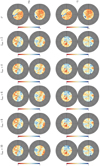 |
Fig. A.1 Orthographic views of the uncertainty (top row) and significance (rows 2–6) maps of Q (left) and U (right) at 353 GHz. The uncertainty maps are in MJy sr−1. The significance maps show the significance of the residuals, defined as (m − d)∕σ per pixel, for the best-fit maps presented in Fig. 8. Conventions are the same as in Fig. 8. |
References
- Alves, M. I. R., Boulanger, F., Ferrière, K., & Montier, L. 2018, A&A, 611, L5 [NASA ADS] [CrossRef] [EDP Sciences] [Google Scholar]
- Andrae, R., Fouesneau, M., Creevey, O., et al. 2018, A&A, 616, A8 [NASA ADS] [CrossRef] [EDP Sciences] [Google Scholar]
- Beck, R., Shukurov, A., Sokoloff, D., & Wielebinski, R. 2003, A&A, 411, 99 [NASA ADS] [CrossRef] [EDP Sciences] [Google Scholar]
- Berdyugin, A., Piirola, V., & Teerikorpi, P. 2014, A&A, 561, A24 [NASA ADS] [CrossRef] [EDP Sciences] [Google Scholar]
- Breitschwerdt, D., Feige, J., Schulreich, M. M., et al. 2016, Nature, 532, 73 [Google Scholar]
- Capitanio, L., Lallement, R., Vergely, J. L., Elyajouri, M., & Monreal-Ibero, A. 2017, A&A, 606, A65 [NASA ADS] [CrossRef] [EDP Sciences] [Google Scholar]
- Chen, B. Q., Huang, Y., Yuan, H. B., et al. 2019, MNRAS, 483, 4277 [NASA ADS] [CrossRef] [Google Scholar]
- Cox, D. P., & Reynolds, R. J. 1987, ARA&A, 25, 303 [NASA ADS] [CrossRef] [Google Scholar]
- de Avillez, M. A., & Breitschwerdt, D. 2009, ApJ, 697, L158 [NASA ADS] [CrossRef] [Google Scholar]
- Dickey, J. M., Landecker, T. L., Thomson, A. J. M., et al. 2019, ApJ, 871, 106 [NASA ADS] [CrossRef] [Google Scholar]
- Farhang, A., van Loon, J. T., Khosroshahi, H. G., Javadi, A., & Bailey, M. 2019, Nat. Astron., 3, 922 [NASA ADS] [CrossRef] [Google Scholar]
- Ferrière, K. 2015, J. Phys. Conf. Ser., 577, 012008 [NASA ADS] [CrossRef] [Google Scholar]
- Foreman-Mackey, D., Conley, A., Meierjurgen Farr, W., et al. 2013, Astrophysics Source Code Library [record ascl:1303.002] [Google Scholar]
- Frisch, P. C., Andersson, B. G., Berdyugin, A., et al. 2012, ApJ, 760, 106 [NASA ADS] [CrossRef] [Google Scholar]
- Gaensler, B. M., Madsen, G. J., Chatterjee, S., & Mao, S. A. 2008, PASA, 25, 184 [NASA ADS] [CrossRef] [Google Scholar]
- Galeazzi, M., Chiao, M., Collier, M. R., et al. 2014, Nature, 512, 171 [NASA ADS] [CrossRef] [Google Scholar]
- Gelman, A., & Rubin, D. B. 1992, Stat. Sci., 7, 457 [Google Scholar]
- Gontcharov, G. A., & Mosenkov, A. V. 2019, MNRAS, 483, 299 [NASA ADS] [CrossRef] [Google Scholar]
- Goodman, J., & Weare, J. 2010, Comm. App. Math. Comp. Sci., 5, 65 [Google Scholar]
- Górski, K. M., Hivon, E., Banday, A. J., et al. 2005, ApJ, 622, 759 [NASA ADS] [CrossRef] [Google Scholar]
- Green, G. M., Schlafly, E., Zucker, C., Speagle, J. S., & Finkbeiner, D. 2019, ApJ, 887, 93 [NASA ADS] [CrossRef] [Google Scholar]
- Gry, C., & Jenkins, E. B. 2014, A&A, 567, A58 [NASA ADS] [CrossRef] [EDP Sciences] [Google Scholar]
- Heiles, C. 1998, The Magnetic Field Near the Local Bubble, eds. D. Breitschwerdt, M. J. Freyberg, & J. Truemper (Berlin: Springer), 506, 227 [NASA ADS] [Google Scholar]
- Lallement, R., Vergely, J. L., Valette, B., et al. 2014, A&A, 561, A91 [NASA ADS] [CrossRef] [EDP Sciences] [Google Scholar]
- Lallement, R., Capitanio, L., Ruiz-Dern, L., et al. 2018, A&A, 616, A132 [NASA ADS] [CrossRef] [EDP Sciences] [Google Scholar]
- Lallement, R., Babusiaux, C., Vergely, J. L., et al. 2019, A&A, 625, A135 [NASA ADS] [CrossRef] [EDP Sciences] [Google Scholar]
- Lee, H. M., & Draine, B. T. 1985, ApJ, 290, 211 [NASA ADS] [CrossRef] [Google Scholar]
- Leike, R. H., & Enßlin, T. A. 2019, A&A, 631, A32 [NASA ADS] [CrossRef] [EDP Sciences] [Google Scholar]
- Leroy, J. L. 1999, A&A, 346, 955 [NASA ADS] [Google Scholar]
- Liu, W., Chiao, M., Collier, M. R., et al. 2017, ApJ, 834, 33 [NASA ADS] [CrossRef] [Google Scholar]
- Maíz-Apellániz, J. 2001, ApJ, 560, L83 [NASA ADS] [CrossRef] [Google Scholar]
- Oppermann, N., Junklewitz, H., Greiner, M., et al. 2015, A&A, 575, A118 [NASA ADS] [CrossRef] [EDP Sciences] [Google Scholar]
- Pelgrims, V. 2019, A&A, 622, A145 [NASA ADS] [CrossRef] [EDP Sciences] [Google Scholar]
- Pelgrims, V., & Macías-Pérez, J. F. 2018, A&A, submitted [arXiv:1807.10516] [Google Scholar]
- Pelgrims, V., Macías-Pérez, J. F., & Ruppin, F. 2018, A&A, submitted [arXiv:1807.10515] [Google Scholar]
- Planck Collaboration Int. XX. 2015, A&A, 576, A105 [NASA ADS] [CrossRef] [EDP Sciences] [Google Scholar]
- Planck Collaboration Int. XXX. 2016, A&A, 586, A133 [NASA ADS] [CrossRef] [EDP Sciences] [Google Scholar]
- Planck Collaboration Int. XLIV. 2016, A&A, 596, A105 [NASA ADS] [CrossRef] [EDP Sciences] [Google Scholar]
- Planck Collaboration III. 2020, A&A, in press, https://doi.org/10.1051/0004-6361/201832909 [Google Scholar]
- Planck Collaboration XI. 2020, A&A, in press, https://doi.org/10.1051/0004-6361/201832618 [Google Scholar]
- Planck Collaboration XII. 2020, A&A, in press, https://doi.org/10.1051/0004-6361/201833885 [Google Scholar]
- Puspitarini, L., Lallement, R., Vergely, J. L., & Snowden, S. L. 2014, A&A, 566, A13 [NASA ADS] [CrossRef] [EDP Sciences] [Google Scholar]
- Remazeilles, M., Delabrouille, J., & Cardoso, J.-F. 2011, MNRAS, 418, 467 [NASA ADS] [CrossRef] [Google Scholar]
- Santos, F. P., Corradi, W., & Reis, W. 2011, ApJ, 728, 104 [NASA ADS] [CrossRef] [Google Scholar]
- Skalidis, R., & Pelgrims, V. 2019, A&A, 631, L11 [NASA ADS] [CrossRef] [EDP Sciences] [Google Scholar]
- Snowden, S. L., Koutroumpa, D., Kuntz, K. D., Lallement, R., & Puspitarini, L. 2015, ApJ, 806, 120 [NASA ADS] [CrossRef] [Google Scholar]
- Sokoloff, D. D., Bykov, A. A., Shukurov, A., et al. 1998, MNRAS, 299, 189 [NASA ADS] [CrossRef] [Google Scholar]
- Vansyngel, F., Boulanger, F., Ghosh, T., et al. 2017, A&A, 603, A62 [NASA ADS] [CrossRef] [EDP Sciences] [Google Scholar]
- Wolleben, M., Landecker, T. L., Carretti, E., et al. 2019, AJ, 158, 44 [NASA ADS] [CrossRef] [Google Scholar]
About 2% of the lines of sight do not present a second inflection point within the radial distance of 400 pc, which delineates the probed ISM volume. 22% have their second inflection point closer than 50 pc from the edge, a distance at which we estimate that the second derivative of the radial profile might be biased by the applied smoothing.
Using the HEALPix convention (https://healpix.jpl.nasa.gov/html/intronode12.htm)
If  with
with
 directly from Eq. (7), the normalization factor α
is computed as
directly from Eq. (7), the normalization factor α
is computed as  where
where  with i
running through all the indices of the concatenated maps.
with i
running through all the indices of the concatenated maps.
The E2E maps were downloaded from https://wiki.cosmos.esa.int/planck-legacy-archive/index.php/Simulation_data#Noise_and_instrumental_effect_residual_maps, smoothed at 80′ and downgraded at Nside = 128 before being co-added to the best-fit maps.
All Tables
Best-fit parameter values of the adjusted magnetic field model for the values of lmax used to model the shape of the LB shell based on the L19 3D extinction map.
Best-fit parameter values and corresponding results of the E2E simulations, for the modeled shapes of the LB shell obtained from the L19 (top) and LE19 (bottom) 3D extinction maps, with lmax = 6.
Comparison of the best-fit magnetic fields for four different models discussed in the text.
All Figures
|
Fig. 1 Crosscuts along the planes XY, XZ, and YZ in the L19 3D dust extinction map. The Sun is at the center. The X axis points from the Sun to the Galactic center at Galactic longitude l = 0°, the Y axis points towards l = 90° and the Z axis points to the North Galactic pole. The Galactic center is to the right in the left and middle panels and back to the reader in the right panel. The color scale shows
|
| In the text | |
|
Fig. 2 Example of radial profiles of differential extinction ( |
| In the text | |
|
Fig. 3 Crosscuts along the planes XY, XZ, and YZ in the L19 3D dust extinction map, with the same conventions as in Fig. 1. The (common) gray scale shows
|
| In the text | |
|
Fig. 4 Full-sky map of (top) the inner surface of the LB shell (rinner) as extracted from the L19 3D extinction map (Sect. 2.2.1) and (bottom) our model of this surface through a spherical harmonic expansion up to lmax = 6 (Sect. 2.2.2). The maps are in Galactic coordinates, the center points towards the Galactic center and longitude increases to the left. |
| In the text | |
|
Fig. 5 Same as for Fig. 3, except that the underlying dust density distribution and the corresponding inner and outer surfaces of the LB shell (red and green lines, respectively) are from the LE19 3D map. Our models of the inner surface (black dotted, dashed and solid lines) are still based on the L19 map. |
| In the text | |
|
Fig. 6 Same as for Fig. 5, except that our models of the inner surface of the LB shell (black dotted, dashed and solid lines) are now based on the LE19 map. |
| In the text | |
|
Fig. 7 Euclidean distances (d, given by Eq. (1)) between several models of the LB shell inner surface as a function of the maximum multipole degree (lmax). The gray dotted line compares the first and final iterations of the iterative procedure discussed in Sect. 2.2.2 and applied to the L19 data. The blue dashed line compares the final models obtained with the L19 and LE19 data. The orange and purple dot-dashed lines compare the final models obtained with the L19 and LE19 data, respectively, with the shape of the LHB from Liu et al. (2017) (see Sect. 2.5). |
| In the text | |
|
Fig. 8 Orthographic views of the Q (left) and U (right) maps at 353 GHz. From top to bottom: Planck PR3 data and best-fit maps corresponding to the modeled shapes of the LB shell obtained from the L19 3D extinction map, with lmax = 2, 4, 6, 8, and 10. The background structures underlying the maps come from the dust column density taken from the data. Units are MJy sr−1. In orthographic views, the North and South Galactic Poles lie at the center of the left and right circles, respectively, the vertical solid radius shows longitude 0°, and the left and right panels touch at l = 90°. The gray area corresponds to the region |b| < 60°, which is notconsidered in the fitting procedure. |
| In the text | |
|
Fig. 9 1D and 2D marginalized posterior distributions of the model free parameters. The modeled shapes of the LB shell are obtained from the L19 3D extinction map, with lmax = 2, 6, and 10. The verticaldashed lines show the 2.5, 50 and 97.5 percentiles. |
| In the text | |
|
Fig. A.1 Orthographic views of the uncertainty (top row) and significance (rows 2–6) maps of Q (left) and U (right) at 353 GHz. The uncertainty maps are in MJy sr−1. The significance maps show the significance of the residuals, defined as (m − d)∕σ per pixel, for the best-fit maps presented in Fig. 8. Conventions are the same as in Fig. 8. |
| In the text | |
Current usage metrics show cumulative count of Article Views (full-text article views including HTML views, PDF and ePub downloads, according to the available data) and Abstracts Views on Vision4Press platform.
Data correspond to usage on the plateform after 2015. The current usage metrics is available 48-96 hours after online publication and is updated daily on week days.
Initial download of the metrics may take a while.