| Issue |
A&A
Volume 689, September 2024
|
|
|---|---|---|
| Article Number | A2 | |
| Number of page(s) | 18 | |
| Section | Interstellar and circumstellar matter | |
| DOI | https://doi.org/10.1051/0004-6361/202450310 | |
| Published online | 27 August 2024 | |
Gamma-ray line emission from the Local Bubble
1
Julius-Maximilians-Universität Würzburg, Fakultät für Physik und Astronomie, Institut für Theoretische Physik und Astrophysik, Lehrstuhl für Astronomie,
Emil-Fischer-Str. 31,
97074
Würzburg,
Germany
e-mail: This email address is being protected from spambots. You need JavaScript enabled to view it.
2
Zentrum für Astronomie und Astrophysik, Technische Universität Berlin,
Hardenbergstr. 36,
10623
Berlin,
Germany
3
RIKEN Nishina Center,
2-1 Hirosawa, Wako,
Saitama
351-0198,
Japan
Received:
10
April
2024
Accepted:
23
May
2024
Abstract
Deep-sea archives that include intermediate-lived radioactive 60Fe particles suggest the occurrence of several recent supernovae inside the present-day volume of the Local Bubble during the last ~10 Myr. The isotope 60Fe is mainly produced in massive stars and ejected in supernova explosions, which should always result in a sizeable yield of 26Al from the same objects. 60Fe and 26Al decay with lifetimes of 3.82 and 1.05 Myr, and emit γ rays at 1332 and 1809 keV, respectively. These γ rays have been measured as diffuse glow of the Milky Way, and would also be expected from inside the Local Bubble as foreground emission. Based on two scenarios, one employing a geometrical model and the other state-of-the-art hydrodynamics simulations, we estimated the expected fluxes of the 1332 and 1809 keV γ-ray lines, as well as the resulting 511 keV line from positron annihilation due to the 26Al β+ decay. We find fluxes in the range of 10−6–10−5 ph cm−2 s−1 for all three lines with isotropic contributions of 10–50%. We show that these fluxes are within reach for the upcoming COSI-SMEX γ-ray telescope over its nominal satellite mission duration of 2 yr. Given the Local Bubble models considered, we conclude that in the case of 10–20 Myr-old superbubbles, the distributions of 60Fe and26 Al are not co-spatial - an assumption usually made in γ-ray data analyses. In fact, this should be taken into account however when analysing individual nearby targets for their 60Fe to26 Al flux ratio as this gauges the stellar evolution models and the age of the superbubbles. A flux ratio measured for the Local Bubble could further constrain models of 60Fe deposition on Earth and its moon.
Key words: ISM: bubbles / gamma rays: diffuse background / gamma rays: ISM
© The Authors 2024
 Open Access article, published by EDP Sciences, under the terms of the Creative Commons Attribution License (https://creativecommons.org/licenses/by/4.0), which permits unrestricted use, distribution, and reproduction in any medium, provided the original work is properly cited.
This article is published in open access under the Subscribe to Open model. This email address is being protected from spambots. You need JavaScript enabled to view it. to support open access publication.
1 Introduction
Measurements of the γ-ray line at 1809 keV from decaying26 Al suggest a quasi-persistent mass of this radioactive isotope of 1.2–2.4 M⊙ distributed throughout the Galaxy (Pleintinger et al. 2023; Siegert et al. 2023). While it is commonly assumed that large parts of this mass originates in massive stars (Knödlseder 1999; Diehl et al. 2006), contributions from classical novae and asymptotic giant branch (AGB) stars may also play a role (e.g. Vasini et al. 2022, suggesting a nova contribution of up to 30%). Being agnostic about the possible contribution from low-mass stars, Siegert et al. (2023) found a core-collapse supernova rate of 1.8–2.8 per century based on comparisons with γ-ray measurements of the 26Al decay line at 1809 keV alone. With their population synthesis model, the mass of radioactive 60Fe could also be estimated, ranging between 1–6 M⊙. Given the γ-ray line measurements of Wang et al. (2020) who detected both decay lines of 60Fe at 1173 and 1332 keV in the Milky Way, this model estimate appears reasonable, but includes large uncertainties.
Data analyses of soft γ-ray emission, such as for nuclear lines, depend on spatial templates that are assumed to represent the emission. Refining these models is then an iterative approach that can also lead to substantial changes in understanding the emission with ever-increasing exposure from the large field-of-view γ-ray telescopes. In a recent work, trying to compare the raw data of the 1809 keV line from INTE-GRAL/SPI with Galactic-scale hydrodynamics simulations (e.g. Fujimoto et al. 2018; Rodgers-Lee et al. 2019; Krause et al. 2021), Pleintinger et al. (2019) found a non-uniform scale height along Galactic longitudes. In particular, the data suggest a scale height distribution that peaks around a few tens of parsecs and then stays rather flat up to, and possibly beyond, 2 kpc. On the one hand, this was surprising as, typically, emission templates with uniform scale heights worked particularly well in γ-ray data analyses (e.g. Knoedlseder et al. 1999; Diehl et al. 2006; Wang et al. 2009, 2020; Siegert 2017; Pleintinger et al. 2019). On the other hand, this can be interpreted as superbubbles that open up towards higher latitudes allowing26 Al to flow towards regions of lower densities (Krause et al. 2021).
Another interpretation of the findings by Pleintinger et al. (2019) is local foreground emission that would be hard to detect as an almost-isotropic component for current coded aperture mask γ-ray telescopes (Siegert et al. 2022b). However, the hints for very large scale heights may point to emission very nearby that is not directly connected to the Galactic background. A natural candidate for such a foreground emission would be the Local Bubble (e.g. Breitschwerdt et al. 1996), the superbubble in which the Solar System is currently located.
This argument is further strengthened by measurements in deep-sea archives that show exceptionally high concentrations of radioactive 60Fe particles in certain layers that cannot have been produced on Earth (e.g. Wallner et al. 2016, 2021). This points to nearby supernova activity within a period of a few million years, similar to the decay times of 60Fe and 26Al. If there had been supernovae within the Local Bubble not too long ago, residual 60Fe and26 Al would still be present and currently decaying, leading to γ-ray emission from all directions. In addition, due to the β+ decay of26 Al, positrons would currently be produced and would presumably annihilate in the bubble walls, creating another γ-ray line at 511 keV.
In this study, we want to investigate how strong the γ-ray line emission from the Local Bubble is at the decay energies of 1809 keV (26Al), 1332 and 1173 keV (60Fe), and 511 keV (positron annihilation). In particular, we study the emission of γ rays owing to the following decay chains and reactions, in which all the lifetimes (τ) and probabilities (p) relevant for this work are indicated:
 (1)
(1)
 (2)
(2)
 (3)
(3)
 (4)
(4)
Because the probabilities of the final 60Ni de-excitation in Eq. (1) are very similar and close to 1.0, we used the 1332 keV line as a surrogate for the expected 60Fe emission. We note that in data analyses, the significance of both lines combined is increased roughly as  (see Sect. 5). The annihilation of positrons with electrons in the environment of the Local Bubble is assumed to be dominated by charge exchange (Ch. ex.) with hydrogen, leading to the intermediate bound state of Positronium (Ps). Depending on the spin state of Ps, either para-Ps or ortho-Ps decays on the nano-second timescale, which results in two 511 keV photons for only para-Ps and a continuous spectrum up to 511 keV for ortho-Ps (Ore & Powell 1949). The direct annihilation with (free) electrons is subdominant, and the cross section for radiative recombination with electrons inside the Local Bubble is several orders of magnitude smaller than for charge exchange. For this reason, we only focus on the most dominant photon emission process in the case of positron annihilation, Eq. (3), and discuss a correction factor for direct annihilation in Sects. 3.1.2 and 3.2.2.
We base our estimates on two modelling assumptions, one from a geometrical point of view (Pelgrims et al. 2020; Zucker et al. 2022) with physical arguments, and one from a hydrodynamics point of view (Schulreich et al. 2023) with detailed setups, both tailored to match the terrestrial deposition of 60Fe. By identifying the total fluxes, their isotropic contribution, and flux ratios as a function of position, we can suggest figures of merit of how to distinguish between different models, and also if it is indeed possible to perform these measurements with future γ-ray telescopes.
This paper is structured as follows: In Sect. 2, we describe previous measurements of the Local Bubble considering size, shape, age, and radioactivity content, as well as recent hydrodynamics simulations tailored to match the radioactive impact on Earth. Section 3 includes the expected photon emission from different γ-ray lines originating from the Local Bubble, including 26Al, 60Fe, and the 511 keV line considering two scenarios. We describe the signal-to-Galactic-background ratio in Sect. 4 to determine emission hot spots and isotropic components. Since current instruments are nearly incapable of measuring isotropic emission, we estimated the detectability of the Local Bubble in these γ-ray lines with the future COSI-SMEX satellite instrument and present the results in Sect. 5. Finally, we discuss our findings in Sect. 6 and conclude in Sect. 7.
2 Local Bubble and Solar vicinity
The Local Bubble is an asymmetric superbubble, that is, a cavity of hot plasma surrounded by a shell of hydrogen and dust, in which the Solar System is currently propagating through. It has been formed by massive stars and supernovae within the last ~20 Myr. Determining the three-dimensional (3D) geometry of the Local Bubble is not trivial (e.g. Lallement et al. 2014), as it relies on accurate measurements of lines of sight to stars in front of and behind the Local Bubble walls. As the number of stars towards higher latitudes becomes smaller, the estimates of the Local Bubble size in different directions becomes more uncertain. In this paper, we use two assumptions for the geometry of the Local Bubble: (1) A measurement-based geometrical model that determines the inner radii of the Local Bubble using a spherical harmonics decomposition (Pelgrims et al. 2020), and (2) hydrodynamics simulations in which the Local Bubble self-consistently forms in an inhomogeneous background medium through feedback processes of those massive stars that perished in nearby stellar populations calculated back over the last 20 Myr (Schulreich et al. 2023). In the following, we briefly describe these two models.
2.1 Recent measurements
Pelgrims et al. (2020) used 3D dust density maps from Lallement et al. (2019) that covers a volume which contains the entire Local Bubble to estimate the inner and outer boundaries of the bubble. In their work, they base the analysis and modelling on the constructed 3D map of dust reddening from Gaia DR2 photometric data in combination with 2MASS measurements to estimate the dust extinction towards stars in all directions. This results in a map that includes the differential extinction as a function of the distance to the Sun, which in turn can be used to estimate the gas density of the Local Bubble. With a narrow sampling of lines of sight from the Sun outwards, Pelgrims et al. (2020) could identify the inner and outer radii of the Local Bubble walls for all viewing angles. The authors note that the outer radii are, sometimes, not reliable, for which reason we only use the inner radii in the following sections. Depending on the direction, the Local Bubble shell thickness ranges between 50 and 150 pc. For inner radii between 80 and 360 pc (Fig. 1), this may be considered rather large as typical wall thicknesses range around 10–30% (e.g. Krause et al. 2013; Krause & Diehl 2014). Interestingly, Pelgrims et al. (2020) found that the cavity appears to be closed in all directions, rather than showing a chimney-like structure which had been suggested in different studies about superbubbles in general (e.g. Krause et al. 2021). In a next step, the measurements of the inner radii are expanded into spherical harmonics with different maximum multipole degrees lmax that adjust the level of complexity of the inner Local Bubble surface. For a given lmax, the internal structure of the Local Bubble are more or less pronounced, and the authors suggest lmax = 6 for further analyses. We will use two cases, 1a with lmax = 40 and 1b with lmax = 6, to illustrate the differences in these assumptions in Sect. 3.1.
Based on the work by Pelgrims et al. (2020), Zucker et al. (2022) discuss the shapes and motions of dense gas and young stars inside and in the vicinity of the Local Bubble. They find that, apparently, all young star-forming regions are close to the surface of the Local Bubble, and that these show an outward motion. To explain this expansive movement, Zucker et al. (2022) suggest a star-burst event near to what is now the centre of the Local Bubble about 14 Myr ago. The subsequent supernovae formed the Local Bubble that is now fragmenting near its boundaries to molecular clouds, hosting the next generations of young stellar clusters. Such a picture is widely known as triggered star formation by stellar winds and supernovae.
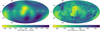 |
Fig. 1 Inner boundaries of the geometrical Local Bubble model as derived by Pelgrims et al. (2020). Shown are two different granularities of the spherical harmomics decomposition with lmax = 6 (left) and lmax = 40 (right). |
2.2 Recent hydrodynamics simulations
The high-resolution 3D hydrodynamics simulations of Schulreich et al. (2023) utilised in this work are an extensive update of those first presented in Schulreich (2015) and are based on the most sophisticated initial conditions for the formation and evolution of the Local Bubble determined to date. These include the number of core-collapse supernova explosions, as well as when and where they occurred, relying on a Gaia EDR3-based stellar census of the Scorpius-Centaurus (Sco-Cen) OB association by Luhman (2022), which has already emerged as the most likely source of most, if not all, of these supernovae in previous studies (e.g. Fuchs et al. 2006). By fitting the initial mass function (IMF) of Kroupa (2001), the total number of missing and thus exploded stars was found to be 14, of which 13 occurred in Upper Centaurus-Lupus and Lower Centaurus-Crux (UCL/LCC), and one in V1062 Sco (both being Sco-Cen populations). The lifetimes of the perished stars and therefore the timing of their explosions – assuming that all members of a population are formed simultaneously - were estimated by interpolating between the rotating stellar evolution tracks for solar metallicity of Ekström et al. (2012) to match the stars’ initial masses, obtained from IMF binning. For deriving the trajectories of the supernova progenitors, a novel Monte Carlo-type approach was developed, for which 10 000 realisations of each progenitor population were back-calculated in time by means of test-particle simulations with a realistic Milky Way potential (Barros et al. 2016). The explosion sites were selected based on the maximum values in six-dimensional phase-space probability distributions constructed from the stellar tracebacks.
The hydrodynamics simulations studied the turbulent transport of the radioisotopes26 Al, 53Mn, 60Fe, and 244Pu1 due to stellar wind and supernova activity in the domain of the present-day Local Bubble, which forms over the last 20Myr (the birth time of the two progenitor populations) in a smoothly stratified modelled local interstellar medium. With all the radioisotopes treated as decaying passive tracers, only 26Al is released by the stellar winds (set up to be age- and initial mass-dependent), for which the yields of Ekström et al. (2012) were used. The supernova yields for 26Al, 53Mn, and 60Fe, on the other hand, were taken from Limongi & Chieffi (2018). Only 244Pu was assumed to be pre-seeded (possibly by a kilonova event prior to the formation of the Local Bubble) in the sense of a two-step scenario (see also e.g. Wang et al. 2021), with its initial concentration reconstructed from fitting the measurements of Wallner et al. (2021) in the uppermost deep-sea crust layers. The Solar System, which, like each of the 14 supernova progenitors, travels as a ‘stellar particle’ along its pre-calculated trajectory, crosses the outer shell of the Local Bubble about 4.6 Myr ago and acts as a 'moving detector' for the radioisotopic fluxes originating from the stellar feedback processes throughout the entire simulation time. Without any real fine-tuning (only the density in the Galactic mid-plane was varied and finally set to 0.7 H cm−3), the numerical calculations are able to reproduce remarkably well the measurements of the four radioisotopes currently available for the time period from the Sun’s entry into the Local Bubble. In addition, its present-day extent and the value of the thermal pressure of the hot plasma in its interior, which was estimated by Snowden et al. (2014) from a combination of disparate observational results, are matched. An even better match to the ~3-Myr-old 60Fe signal was found when the massive star responsible for the most recent supernova (about 0.88 Myr ago) was removed from the simulation, implying a slight deviation from the most probable initial mass spectrum underlying the original scenario. We consider the 14-supernovae scenario as case 2a and the alternative simulation in which the last supernova was simply taken out as case 2b.
3 γ-ray line emission from the Local Bubble
For the 26Al and subsequent 511 keV emission, and 60Fe γ-ray line emission, we are considering two case studies: In the first case (case 1), we use the geometric model as inferred from measurements by Pelgrims et al. (2020) (see also Zucker et al. 2022), in combination with the estimated 60Fe deposit as determined in Chaikin et al. (2022), to calculate the emissivity of26 Al, its decay positrons, and 60Fe γ-rays. The second case (case 2) is based on hydrodynamics simulations by Schulreich et al. (2023), who tailored their simulations to match not only the 60Fe deposit on Earth but in addition26 Al, 53Mn, and 244Pu influxes from past supernovae in the Solar neighbourhood. The premises for both cases are vastly different, so that the final emissivities and γ-ray flux maps will provide a reasonable range of possibilities of how the Local Bubble may look like as seen from an observer inside at the position of the Sun. We will discuss the two cases separately in the following, for the three γ-ray lines considered, 1809 keV from 26Al, 1332 keV from 60Fe (the flux and appearance from the 1173 keV line from 60Fe is identical), and 511 keV from Ps-decay.
3.1 Case 1: Geometric model and 60Fe deposit
The geometric model of Pelgrims et al. (2020) delivers the inner boundaries of the Local Bubble, described as a function of distance to the Sun in the centre of the coordinate system. Their model is provided as a HEALPix array with a side length of 128, resulting in 196 608 values for the three Cartesian directions, x, y, and ɀ. Pelgrims et al. (2020) provide different levels of granularity in the reconstruction of the inner surface of the bubble as described by an expansion of the measurements into spherical harmonics up to multipoles lmax of 2, 4, 6, 8, 10, 20, 30, and 40. For illustration purpose in this work, we use lmax = 6 and 40. The former is a reasonable trade-off between the granularity of the shell and the expected turbulence. We use the latter as an extreme case, that should however not be over-interpreted because the maps of distances, R(ℓ, b), show some ‘ringing effect’2 (Pelgrims, priv. comm.), but which results in γ-ray flux maps that are more in line with the hydrodynamics simulations naturally including turbulence on the pc scale (see Sect. 3.2).
In what follows, we will always construct all-sky maps on a 1°×1° (rectangular) pixel grid, that is, we will calculate the differential flux in units of ph cm−2 s−1 sr−1 for each of the 360 × 180 = 64 800 pixels and each process. In case 1 this means we need to define an emissivity ϵ(x, y, ɀ) in units of cm−3 s−1 inside the inner boundaries for 60Fe and 26Al, and the outer boundaries for 511 keV. The first step is then interpolating the maps of radii from HEALPix in Cartesian into spherical coordinates spanned by the line of sight variable s (from the point of the observer to infinity) and the two Galactic coordinates of longitude ℓ and latitude b. The emissivity profiles that we define (see below) are then also transformed from Cartesian to spherical coordinates, ϵ(x, y, ɀ) → ϵ(s, ℓ, b), from which the line-of-sight integration is performed as
 (5)
(5)
where the line of sight is defined as
 (6)
(6)
with (x, y, ɀ)⊙ being the coordinates of the Sun which is taken here to be the position of the observer. The coordinates are chosen so that the positive x-direction points towards the Galactic centre, the positive ɀ-direction to the Galactic north pole, and the positive y-direction to ℓ = 90°. Pelgrims et al. (2020) used (x, y, ɀ)⊙ = (0, 0, 0) as the coordinates of the Sun, which we keep for case 1a and 1b (for a more realistic Sun position, see Bennett & Bovy 2018, see also Sect. 3.2). The comparison between the geometrical model and the hydrodynamics simulation is then only biased by the observer position with a vertical difference of 20.8 pc.
The two geometries of lmax = 40 and lmax = 6 differ only slightly, with their minimum and maximum radii being larger and smaller, respectively. We refer to cases 1a and 1b for lmax = 40 and lmax = 6 in the following but will restrict the illustrations to case 1a.
3.1.1 60Fe and 26Al emissivities
We calculate the luminosity of a radioactive isotope i inside the Local Bubble as follows. Given its total ejecta mass Mi, its lifetime τi, its atomic mass mi, and the probability to emit a γ-ray photon pi, we find the total luminosity Li(t) as a function of time t as
 (7)
(7)
where t0 is the time at which the isotope is ejected (or produced). Since the Local Bubble is not a distant point source, we need to take into account both, the expected profile of isotope i inside, and the boundaries of the bubble to identify the limits of the line-of-sight integration. It has been suggested that the ejected mass from supernovae and stellar winds in super-bubbles quickly homogenise on a timescale of ~Myr (Krause et al. 2013; Krause & Diehl 2014) from which a constant emis-sivity could be expected. Here, we use a slightly more complex model and convert the time-dependence of Eq. (7) into a radial dependence using a typical sound velocity inside the bubble of vturb ~ 300 km s−1, from which we define the emissivity for the isotope i as
 (8)
(8)
where (x, y, ɀ)SN is the position of a supernova with age tSN so that r(xSN, ySN, ZSN) =  .The normalisation factor ϵ0,i· is obtained by calculating the ‘effective volume’ V of the Local Bubble, having its boundary at R(ℓ, b),
 (9)
(9)
so that finally
 (10)
(10)
With the sound speed of ~300 km s−1, the lifetimes of 26Al and 60Fe of τ26 = 1.05 Myr and τ60 = 3.8 Myr, respectively, and the typical radial scale of the Local Bubble between 100 and 300 pc, the second exponential term in Eq. (8) amounts to a decrease from the centre to the edges of 0.7–0.4 in the case of 26Al, and 0.9–0.8 for 60Fe. This means, there will be a large fraction of the emissivity distributed isotropically, but still some ‘hotspot’ left, indicating of where the last supernova happened. It is also clear already from this consideration that the distributions of 26Al and 60Fe are not completely co-spatial, as typically assumed in γ-ray data analyses (e.g. Wang et al. 2007, 2020; Siegert et al. 2023). As will be discussed in Sect. 3.2, it is in fact possible to identify the position of the last supernova by hotspots in the 1809 keV flux map.
In the model of Chaikin et al. (2022) two supernovae 3 and 7 Myr ago are held responsible for the 60Fe measured by Wallner et al. (2021) in deep-sea samples. The positions of these two supernovae are not provided by the authors. We mimic the position of the 3 Myr-old supernova from the positions derived in Schulreich et al. (2023) (see also Sect. 3.2) that occurred at (x, y, z) = (40.9, −65.9, 19.5) pc and about 92.2 pc away at the time of the explosion, and the 7 Myr-old supernova at (x, y, z) = (113.1,−15.6,7.3)pc, about 220.9pc away. Thus, we calculate two emissivity profiles by using Eq. (8) and simply add them. We note that the mixing inside the Local Bubble and in particular its shape is bound to change within the last 7 Myr. For the sake of simplicity in this case 1, we nevertheless keep it at this straight-forward model, also because the models for γ-ray observations typically use these simple assumptions (see also the discussion about these assumptions in Sect. 6). While Chaikin et al. (2022) discuss the effects of the uptake of dust particles on Earth which would lead to a range of plausible ejecta masses, we keep the 60Fe yield per supernova for our geometrical model to their canonical value of 10−4 M⊙. Considering this 60Fe ejecta mass, we need to consider the possible impacts of the progenitor stars that may alter the yields of 26Al. These include the rotational velocity, the metallicity, and to a lesser extent the binarity. The rotational velocities of the progenitor stars are unknown, but given that they must have been O- or B-type stars to form the Local Bubble, we can estimate an expectation value and a range of possible rotational velocities from the catalogue of Głebocki & Gnacinski (2005). We find a range of 140 ± 90 km s−1 for O-and 135 ± 105 km s−1 for B-type stars, which we combine into a range of 30–240 km s−1. This covers large parts of the calculations by Limongi & Chieffi (2018) with a velocity grid of 0, 150, and 300km s−1. The metallicity of these young objects are even less constrained: Given the metallicity gradient of the Milky Way by Cheng et al. (2012), for example, one could estimate the average metallicity around the Solar circle to be about − [Fe/H] = 0.29–0.90. However, since the Sun already has solar metallicity by definition, any much younger object might have super-solar metallicity, which would be difficult to estimate. Limongi & Chieffi (2018) calculated a grid of metallicities ranging between 10−3, 10−2, 10−1, and 100, so that any super-solar yield would require an extrapolation from the available ones. As a conservative approach, we will use a metallicity of [Fe/H] = 0 to estimate the masses of the progenitor stars. Using all the above arguments, we find that the two progenitor stars that exploded 3 and 7 Myr ago must have had initial masses of 13–25 M⊙, assuming the yield model by Limongi & Chieffi (2018). The resulting yields for 60Fe and26 Al are then 1.0 × 10⁻⁴ M⊙ (by definition) and (1.6–13.0) × 10−5 M⊙, respectively.
3.1.2 Positron annihilation from 26Al
The isotope26 Al decays with a probability of pβ+ = 0.82 via β+-decay and thereby emits a positron with a mean kinetic energy of 543 keV in the β-decay spectrum up to an end point energy of 1173 keV. The positron is therefore at most mildly relativis-tic with γ ≤ 3.3. Low-energy positron propagation is hardly understood, that is, if they propagate ballistically, diffusively, or if magneto-hydrodynamic waves have a large impact (see Jean et al. 2009, for details). From the energy losses, here mainly ionisation and Coulomb losses, as well as the annihilation rates at different temperatures of the interstellar medium (Guessoum et al. 2005), we estimate where the positrons tend to annihilate in the context of a superbubble like the Local Bubble.
The path length of a positron from 26Al with maximum Lorentz-factor of γmax = 3.3 inside a superbubble with a hydrogen density of nH,mm ~ 10-4 cm−3 is of the order of Rball,max ~ 100 Mpc – inside of bubble walls with a density of nH,mm ~ 101 cm−3 of the order of Rball,max ~ 1 kpc. Positrons certainly propagate along the (possibly tangled) magnetic field lines in superbubbles, which reduces effective distances by magnetic diffusion. We approximate the diffusion length scale by  , where κ ~ 2–3, depending on the directionality of the magnetic field to diffuse in, D is the (unknown) diffusion coefficient, and v+ is the Alfvén speed. We note that the Alfvén speed differs in detail depending on the magnetic field strength, and the density; for an order of magnitude estimate, we will use the range of 101– 103 km s−1 . Typical values of D for GeV positrons range around 1027 cm2 s−1 , which we use here as canonically value also for mildly relativistic positrons (see Martin et al. 2012, for different scenarios on how the low-energy positron propagation might be realised in the interstellar medium), so that the diffusion length scale is of the order of 100–102 pc for this collisionless transport model. The effective distance can then be approximated as
  which ranges from 1 pc to several 100 kpc. We note that the propagation of low-energy positrons is not well understood and that different scenarios, such as collision-less transport, intermediate inhomogeneous transport, and pure ballistic transport may all be realised in nature (Martin et al. 2012). Thus, in the latter case, positrons would diffuse through the Local Bubble walls into the next bubble, from which they might also escape, so that the annihilation emission may not be traced back to the production site. In the first case, the positrons would annihilate rather quickly once they reach a density high enough to lose their kinetic energy efficiently. As the last case may be interesting on a global, Galactic-wide, picture, we will only consider and discuss the first case in this work.
In order to estimate the emissivity profile of annihilating positrons, we consider again the effect of diffusion, now in competition with the effect of annihilation. The number density of annihilating positrons can be described as a function of radial coordinate as
 (11)
(11)
where Ḋ(r) is the diffusion term of a positron propagation from a spherical shell at r into a shell at r + dr, and reads
![Mathematical equation: $\dot D(r) = 4\pi \v (r)\left[ {{n^*}(r){r^2} - {n^*}(r + {\rm{d}}r){{(r + {\rm{d}}r)}^2}} \right]{\rm{, }}$](/articles/aa/full_html/2024/09/aa50310-24/aa50310-24-eq16.png) (12)
(12)
with  being the diffusion velocity. In Eq. (11),
  is the annihilation term which removes particles with an annihilation rate
  in a shell at r with a hydrogen number density nH(r), so that
 (13)
(13)
We note that the annihilation rates  (Guessoum et al. 2005) per target density, that is, in units of cm3 s−1, will automatically depend on the position as well as the temperature changes across the bubble. Assuming a steady state, that is, setting the left hand side of Eq. (11) to zero, we derive the general solution of the density of annihilating positrons as
![Mathematical equation: ${n^*}(r) = n_0^*\exp \left\{ { - 2\int_{{r_0}}^r {\left[ {{1 \over r} + {{\kappa \dot a(T(r)){n_{\rm{H}}}(r)} \over {2D}}r} \right]} {\rm{d}}r} \right\}{\rm{. }}$](/articles/aa/full_html/2024/09/aa50310-24/aa50310-24-eq22.png) (14)
(14)
A short derivation of this general solution is found in Appendix A. The impact of the diffusion coefficient is now estimated by solving the integral for different conditions of a superbubble. The annihilation rates per target density,  , are chosen from Guessoum et al. (2005); we restrict ourselves to the cases of charge exchange (Ch. ex.) with hydrogen, radiative recombination (rad. rec.) with electrons, and direct annihilation in flight (daf). At a specific position with high density, such as near the bubble walls with nH ~ 1 cm−3 and a temperature of T ~ 104 K, the factor
  obtains an order of magnitude of 10−10 s−1. With the diffusion coefficient of 1028 cm2 s−1, the second term in the integral of Eq. (14) reduces to ~10−38 cm−2 ≈ 0.1 pc−2. This means that the propagation is hampered severely beyond the pc scale. Consequently, we can assume that the annihilation of positrons – once they are cooled down sufficiently – is instantaneous. Finally, assuming a smooth step function (Fermi function) in density and temperature, the typical width of such an instantaneous positron annihilation region is at most 1 pc and exponentially decreasing. The exponential decrease depends inversely proportional on D (see Eq. (14)) with D ~ 1028 cm2 s−1 leading to a sharp profile with at most 10−3 pc width. Such a profile will essentially outline the inner boundaries of the geometrical Local Bubble model.
The absolute luminosity of the annihilating positrons is derived from the 26Al ejecta mass and the delay between the supernova explosion plus the propagation time scale (cooling time),
 (15)
(15)
which evaluates to at most 0.4 Myr in the case of nH ~ 10−4 cm−3. We use this value as the maximum delay time tprop of positrons which are seen to annihilate now, so that the annihilation luminosity reads
![Mathematical equation: ${L_ \pm } \approx \sum\limits_{k = 1}^2 {\left[ {{{{M_{26,k}}{p_{\beta + }}} \over {{m_{26}}{\tau _{26}}}}\exp \left( { - {{{t_k}} \over {{\tau _{26}}}}} \right)} \right]} \exp \left( { + {{{t_{{\rm{prop }}}}} \over {{\tau _{26}}}}} \right),$](/articles/aa/full_html/2024/09/aa50310-24/aa50310-24-eq26.png) (16)
(16)
where t1 = 3 Myr and t2 = 7 Myr are the ages of the two supernovae, and M26,1 = M26,2 = (1.6–13.0) × 10−5M⊙ are the respective 26Al yields. Equation (16) then evaluates to 1036– 1037 e+ s−1. This luminosity will be distributed on a shell about 1 pc thick, which is shaped as the Local Bubble, resulting in an emissivity of ~10−23–10−22 e+ cm−3 s−1. We discuss the systematic uncertainties of this model in Sect. 6.
3.2 Case 2: Hydrodynamics simulations
In order to apply the line-of-sight integration technique described in Sect. 3.1 without major modifications to those snapshots of the hydrodynamics simulations by Schulreich et al. (2023) that capture the Local Bubble at the present time, we interpolated the values from the adaptively gridded Cartesian mesh onto a uniform Cartesian one having the same resolution as the finest grid refinement level. As a result, the edge length, Δx, of each cubic grid cell is about 0.781 pc, which translates into a cell volume of ΔV = (Δx)3 ≈ 0.477 pc3. The starting point of the integration in Eq. (6) is now the actual location of the Sun at (x, y, ɀ)⊙ ≈ (0, 0, 20.8) pc according to Bennett & Bovy (2018), which was also used in the simulations by Schulreich et al. (2023). Of course, the observer can, in principle, be placed at any point, even outside the Local Bubble. We demonstrate this in Sect. 6.3 where we briefly examine what a 10–20 Myr-old superbubble, reminiscent of the Local Bubble, would look like at a distance of a few hundred parsecs.
Before calculating the emissivities for the intermediate-lived radioisotopes and for positron annihilation, we investigate where the two isotopes are found in relation to the overall gas density. To do so, we derived the cell-averaged hydrogen number density, nH(x, y, ɀ) = p(x,y, z) X/mp, and the mass of isotope i, Mi(x, y, z) = ρi(x, y, ɀ) ΔV, from the simulation data, where p is the (total) gas mass density, X ≈ 0.707 is the hydrogen mass fraction, mp is the proton mass, and ρi is the mass density of isotope i. Binning nH logarithmically in 1000 steps between 10−5 and 101 cm−3, we obtain bimodal mass distributions for both radioisotopes peaking around 10−4 and 100 cm−3, which corresponds to the diluted Local Bubble interior and its dense outer shell, respectively. In regions with gas densities between 10−3 and 10−1 cm−3, significantly fewer radioisotopes are present. Furthermore, we separately sum the 26Al and 60Fe masses found in each hydrogen number density bin. The resulting distributions and cumulative distributions are shown in Fig. 2. It can be seen that most (~80%) of the 60Fe is found in the denser material (nH ≳ 10−1 cm−3), whereas more than ~50% of26 Al is found in more diluted gas phases (nH ≲ 10−1 cm−3; see Fig. 2, right). Deviations are due to the significantly different decay times of the two radioisotopes, as well as their explosive yields, which not only show strongly divergent dependencies on the initial masses and thus explosion times of the Local Bubble progenitor stars, but are also generally lower for 26Al than for 60Fe (see Table 2 in Schulreich et al. 2023). Furthermore, in the model only supernovae contribute to the 60Fe present today, while for 26Al also stellar winds have an impact, which only cease before 0.88 Myr (case 2a) or before 1.68 Myr (case 2b), the times of the last supernova explosions. All this is reflected in a relatively balanced distribution between cavity and supershell for 26Al, whereas 60Fe, which is generally present in higher masses, is found proportionally more in the supershell. As a consequence, the 26Al and 60Fe ejecta are not co-spatial, which, however, is a typically assumption made in γ-ray data analyses (e.g. Wang et al. 2007, 2020; Siegert et al. 2023). We further discuss the implications of this finding in Sect. 6.
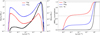 |
Fig. 2 Mass distributions in the Local Bubble. Left: mass distributions of hydrogen (black; left axis), and 26Al (red) and 60Fe (blue; both isotopes right axis) as a function of nH in the hydrodynamics simulation by Schulreich et al. (2023). Note that the right axis is scaled by 10−9 to the left axis to allow a visual comparison. Right: cumulative distribution of the hydrogen, 26Al and 60Fe masses from the left panel with maximum (total) masses of 3.5 × 10⁵ M⊙, 1.6 × 10⁻⁵ M⊙ and 4.9 × 10⁻⁴ M⊙, respectively. Only cells for which the flow speed is higher than 1 km s−1 are used to ensure that the static background medium is not considered as part of the Local Bubble. |
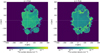 |
Fig. 3 Slices at y = 0 pc through the Schulreich et al. (2023) simulation for the number densities of 26Al (left) and 60Fe (right). It is evident that 60Fe is mostly found along the bubble walls whereas26 Al has also a large contribution of mass in the bubble’s hot phase. The position of the Sun is marked with dashed grey lines at ɀ = 20.8 pc. |
3.2.1 60Fe and 26Al emissivities
We show slices of the Schulreich et al. (2023) hydro-simulation at y = 0 pc for the 26Al and 60Fe number densities in Fig. 3. Also in this representation it is evident that the distribution between the superbubble interior and shell is more balanced for26 Al than for 60Fe, of which relatively more mass could be swept into the shell, primarily by supernova blast waves. From the masses as a function of Cartesian coordinates, we can calculate the γ-ray emissivities in a straightforward manner (cf. Eq. (10)),
 (17)
(17)
from which the flux as a function of longitude and latitude is calculated by Eq. (5).
3.2.2 Positron annihilation from 26Al
Similar to case 1, we will estimate where the positrons from26 Al annihilate in the Local Bubble, given the temperature and density in the simulation. The minimum and maximum temperatures in the simulation are 8000 K and 27.8 MK, respectively. The effect of diffusion will be treated in the same way as before, so that we assume instantaneous annihilation in regions with a preferential combination of the annihilation rate and target density. In Fig. 4, we show slices at y = 0 through the simulated hydrogen number density and temperature distribution in the Local Bubble region. Naturally, one would expect the positrons to annihilate whenever they reach a gas parcel with sufficiently high density and low temperature. Positrons undergo annihilation with neutral hydrogen via charge exchange, taking the electron from the hydrogen atom, to build Ps. However, also annihilations with free electrons can occur, depending on the energy of the positrons and the density of electrons. Since the electron density is not available in this simulation, we restrict ourselves to the case of charge exchange with hydrogen since it is anyway the most probable annihilation channel (see Fig. 5).
At the bubble walls with temperatures around 104 K, the charge exchange with hydrogen is about two orders of magnitude more probable than the direct annihilation or radiative recombination with electrons. For higher temperatures, around the peak of the annihilation rates at 2 × 10⁵ K, the probability is even 105 times greater for charge exchange. For very high temperatures, beyond ~2 MK, where all hydrogen can be expected to be ionised, the charge exchange naturally drops to zero, and radiative recombination with free electrons would take over as the dominant channel. However, the annihilation rate at these high temperatures and the available number of electrons to annihilate with (assuming a one-to-one correlation between protons and electrons), will make the contribution to the γ-ray signal completely negligible.
For the positron emissivity ϵ±(x, y, ɀ) in units of ϵ+ cm−3 s−1, we calculate 16 logarithmic temperature bins from 8000 K to 27.8 MK to assign an annihilation rate to each (x, y, ɀ)-pixel. By multiplying with the cell-averaged hydrogen number densities, we can estimate the weights for the positron annihilation rates
 (18)
(18)
which is shown in Fig. 6 when converted to a positron luminosity L±(x, y, ɀ). The exact number of positrons annihilating now would, again, require the 26Al positron production rate, the propagation time, and annihilation time to be estimated. For simplicity, we assume that the 26Al positron production rate now will result in the positron annihilation rate now,  , where
![Mathematical equation: ${L_{\beta + }} = \sum\limits_{x,y,z} {\left[ {{{{M_{26}}(x,y,z){p_{\beta + }}} \over {{m_{26}}{\tau _{26}}}}} \right]} \approx 1.9 \times {10^{37}}{{\rm{e}}^ + }{{\rm{s}}^{ - 1}}.$](/articles/aa/full_html/2024/09/aa50310-24/aa50310-24-eq30.png) (19)
(19)
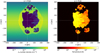 |
Fig. 4 Slices at y = 0 pc through the Schulreich et al. (2023) simulation for the neutral hydrogen number density (left) and the temperature (right). The gas outside the Local Bubble is shaped according to the Galactic plane density distribution, decreasing exponentially towards higher |ɀ|. Small clumps of higher-density gas inside the bubble are visible in both panels, for example around (x, ɀ) = (80, −20) pc. The hot gas is naturally correlated with thin phases of the ISM, and the bubble walls are at a temperature of 8000 K or below. The position of the Sun is marked with dashed grey lines at ɀ = 20.8 pc. |
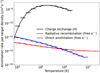 |
Fig. 5 Positron annihilation rates per target density for the processes relevant in this study. The values (solid lines) are taken from Guessoum et al. (2005) and were rebinned (steps) for the purpose of assigning rates in the hydrodynamics simulation by Schulreich et al. (2023). |
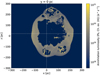 |
Fig. 6 Annihilation luminosity expected in the simulation by Schulreich et al. (2023) from only the charge exchange annihilation channel. Shown is the cell-averaged total luminosity for a slice through y = 0 pc. Clearly, boundary of the supershell shows the highest luminosity, together with the clouds inside the bubble. We again use the condition that the flow velocity must be larger than 1 km s−1 to distinguish the bubble from the background medium (see also Fig. 2). |
4 γ-ray line images from the Local Bubble
We apply Eq. (5) for the γ-ray line of 26Al at 1808.63 keV, the line of 60Fe at 1332.5 keV, and the positron annihilation line originating only from 26Al decay at 511 keV to the two previously discussed cases. We compare the images of case 1a and case 2a side by side for each line and summarise the properties of the models in Table 1.
4.1 26Al emission at 1809 keV
In Fig. 7 we show the comparison of the resulting 1809 keV γ-ray line maps from the decay of 26Al between case 1a with maximal structure (left) and case 2a with 14 supernovae (right). Clearly, because the spatial resolution of the hydro-simulation is much higher than that of the geometrical model, there are more structures visible in the line-of-sight integrated map of the simulation. This will be similar throughout the comparisons and we omit repeating this statement in the following. In the map of case 2a, many of the ‘fingers’ from Fig. 3 are now visible as framed features. The direction, albeit not the distance, of the last supernova is also evident as the region between −140° ≲ ℓ ≲ −20° and −40° ≲ b ≲ +30° is brighter than the remaining sky. Due to the26 Al lifetime of 1.05 Myr, the contribution from the last supernova, as well as from the progenitor’s winds, did not yet homogenise inside the bubble as opposed to the case for 60Fe (see Fig. 8, right). We mimic this behaviour in the geometrical model (case 1), and placed the more recent of the two super-novae considered (3 Myr) at (x,y,z)SN = (40.9, −65.9, 19.5) pc (see Table 2 in Schulreich et al. 2023), which leads to brighter emission in the same regions in the left image, compared to the remaining sky. Likewise, the same effect is visible in the geometric model of 60Fe (see Fig. 8, left), which only appears slightly more homogeneous due to the longer lifetime of 60Fe.
The total 1809 keV γ-ray line fluxes integrated across the entire sky for case 1a and case 2a are 3.3 × 10⁻⁶ ph cm−2 s−1 and 19.5 × 10⁻⁶ ph cm−2 s−1, respectively. The total isotropic part in each image, calculated by
 (20)
(20)
is 1.3 × 10⁻⁶ ph cm−2 s−1 (39%) and 8.7 × 10⁻⁶ ph cm−2 s−1 (44%), respectively. Although the total fluxes differ by a factor of ~6, the isotropic fraction of the emission models are similar between 40 and 50%. Comparing cases 1a and 1b, the fluxes are similar, with the isotropic contribution to be enhanced by 10% due to the smoother reconstruction of the inner radii. As opposed to case 1, the difference between case 2a and case 2b is almost a factor of three in total flux of the26 Al line, mainly because the last supernova has been simply taken out. Then, the isotropic contribution is reduced by ~15% because much of the 26Al has mixed with the bubble walls. Clearly, the impact of the most recent supernova is, expectedly, the largest and would gauge all measurements. The differences and systematic uncertainties in the estimates will be further discussed in Sect. 6.
Summary of γ-ray line fluxes from the Local Bubble.
4.2 60Fe emission at 1332keV
In Fig.8, we show the comparison of the resulting 1332keV γ-ray line maps from the decay of 60Fe between case 1a with maximal structure (left) and case 2a with 14 supernovae (right). As opposed to the general belief that26 Al and 60Fe are co-spatial inside of superbubbles, we clearly find a different appearance between the isotopes. This is true for both cases, although the hydro-simulations provide a better point of argumentation for 60Fe. In the case of 60Fe, mostly the high-density regions are protruding features, now outlining the boundaries at the super-bubble walls. These ring-like structures are projections of the irregularities of the superbubble, created probably by thermal and hydrodynamic instabilities as well as additional pressure from individual supernovae. This leads to a more homogeneous appearance, even though individual high density features, such as around ℓ ~ 135°, b ~ 65° can outshine the remaining sky by factors of a few. The γ-ray maps in 1332 keV show no strong preferred direction of the flux, apart from the different distances to wall edges (left) leading to a contrast of at most ~6, and apart from high density regions which may be prone to forming new stars (right), leading to a contrast of at most ~15.
The total 1332keV γ-ray line fluxes integrated across the entire sky for case 1a and case 2a are 4.6 × 10⁻⁶ ph cm−2s−1 and 42.2 × 10⁻⁶ ph cm−2 s−1, respectively. The total isotropic part in each image is 1.7 × 10⁻⁶ ph cm−2 s−1 (36%) and 13.3 × 10⁻⁶ ph cm−2 s−1 (31%), respectively. Again, the total fluxes differ by a factor of ~9 but the isotropic fraction of the emission models are similar between 30 and 40%. Comparing case 1a to 1b leads again to a similar total flux and slightly increased isotropic ratio as the boundaries are smoother. Likewise, case 2b is showing a ~25% lower flux than case 2a owing to the removal of the last supernova. This reduction in 60Fe line flux is not as strong as for 26Al because of the longer lifetime of 60Fe. More differences and systematic uncertainties will be further discussed in Sect. 6.
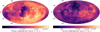 |
Fig. 7 Expected all-sky maps from the decay of 26Al at 1809 keV in the Local Bubble. Left: case 1a of the geometrical model with a total flux of 3.3 × 10⁻⁶ ph cm−2 s−1. Right: case 2a of the hydrodynamics simulation with a total flux of 19.5 × 10⁻⁶ ph cm−2 s−1. See text for discussion and details. |
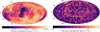 |
Fig. 8 Same as Fig.7 but for the γ-ray line at 1332keV from 60Fe. The total fluxes are 4.6 × 10⁻⁶ ph cm−2s−1 and 42.2 × 10⁻⁶ ph cm−2s−1, respectively. |
4.3 Positron annihilation emission
The positron annihilation images in Fig. 9 are almost similar to the ‘negatives’ of the 26Al images (Fig. 7). This is expected from the distance to the bubble walls where most of the positron annihilation should happen: a bubble wall that is farther away leads to more 26Al along the line of sight to integrate over and consequently a larger 1809 keV flux, but at the same time to a smaller positron annihilation flux as it scales per inverse distance squared. In case 1, this is clearer visible compared to case 2 with the large nearby feature around −5° ≲ ℓ ≲ +45° and −30° ≲ b ≲ +45°. The positron annihilation image of case 2a appears more homogeneous than the 26Al map. This is also understandable as the simulation is bound by a large density in the Galactic plane (see Fig. 2, left). We set a limit to the annihilation belonging to the Local Bubble wherever the flow velocity is above 1 km s−1. In doing so, we set a physically motivated boundary for where we assume positron annihilation to happen if it originated from only 26Al inside the Local Bubble. Clearly, the details in the resulting maps of case 2 originate in the high spatial resolution of the hydrodynamics simulation.
In Fig. 9, we show the positron flux that will undergo charge exchange with hydrogen, not the positron annihilation flux directly. By charge exchange, one positron will capture one electron to form Ps. Depending on the spin state, Ps will either decay into two photons yielding a 511 keV line (para-Ps), or into three photons yielding a rising continuum up to 511 keV (ortho-Ps) (Ore & Powell 1949, see also Eqs. (3)–(4)). The maximum quantum-statistical ratio between the luminosities (and therefore fluxes) of ortho- and para-Ps is 4.5 : 1, as para-Ps is formed 1/4 of the time resulting in 2 photons, and ortho-Ps 3/4 of the time resulting in 3 photons. The total Ps decay flux (para-Ps and 511 keV line direct plus ortho-Ps) is therefore calculated from the positron flux as
![Mathematical equation: ${F_ \pm } = {F_{511}} + {F_{{\rm{oPs}}}} = \left[ {2{1 \over 4}{f_{{\rm{Ps}}}} + 2\left( {1 - {f_{{\rm{Ps}}}}} \right)} \right]{F_{{{\rm{e}}^ + }}} + 3{3 \over 4}{f_{{\rm{P}}{{\rm{s}}_{\rm{s}}}}}{F_{{{\rm{e}}^ + }}},$](/articles/aa/full_html/2024/09/aa50310-24/aa50310-24-eq32.png) (21)
(21)
from which the para-Ps (plus 511 keV line) and ortho-Ps flux (continuum) contributions are readily seen (Brown & Leventhal 1987). Using the above definition includes the Ps fraction ƒPs, which is expected to be 0.955 for a completely neutral hydrogen medium (Guessoum et al. 2005). Considering only the 511 keV line, we obtain a conversion of  3.
3.
The total 511 keV γ-ray line fluxes integrated across the entire sky for case 1a and case 2a are then 21.4 × 10⁻⁶ ph cm−2 s−1 and 2.0 × 10⁻⁶ ph cm−2 s−1, respectively. The total isotropic part in each image is 5.3 × 10⁻⁶ ph cm−2 s−1 (25%) and 0.2 × 10⁻⁶ ph cm−2 s−1 (13%), respectively. The total fluxes differ by a factor of ~11, and the isotropic fraction of the emission models are again similar, now being between 15 and 25%. The differences between case 1a and 1b are, again, similar to the previous γ-ray lines, with a ~15% increase in the isotropic ratio due to the smoother Local Bubble boundaries. Surprisingly, cases 2a and 2b are almost identical although the 26Al input from the last supernova is missing in case 2b. This may be understood as a geometrical effect as the largest parts of the annihilation flux originate in the thick bubble walls rather than in the first few par-secs (see Fig. 6). Further differences and systematic uncertainties will be discussed in Sect. 6.
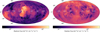 |
Fig. 9 Same as Fig. 7 but for the positron flux. The conversion to 511 keV flux is a factor of 0.568 (see text). The total 511 keV line fluxes are then 21.4 × 10⁻⁶ ph cm−2 s−1 and 2.0 × 10⁻⁶ ph cm−2 s−1, respectively. |
4.4 Total γ-ray line emission: Astrophysical background and Local Bubble foreground
The total γ-ray line fluxes, integrated over the whole sky, of the Local Bubble are summarised in Table 1. Compared to the Milky Way emission in the three γ-ray lines, the Local Bubble flux contribution is marginal, but not negligible. In Pleintinger et al. (2023), the total26 Al 1809 keV line flux has been measured as  , that is, about a factor of 90–600 times brighter than the Local Bubble alone. The total 60Fe flux at 1332 keV has been measured by Wang et al. (2020) to be around
  , which is about 7–70 times brighter than the Local Bubble. It is clear from these numbers alone that detecting the Local Bubble with future γ-ray telescopes (see Sect. 5) will require a careful treatment. However, the almost-isotropic part of this nearby emission as well as the (relatively) stronger flux at very high latitudes (|b| ≳ 60°) from the Local Bubble compared to the Milky Way (mostly confined to |b| ≲ 60°, see Pleintinger et al. 2019; Krause et al. 2021; Siegert et al. 2023) provides some leverage to distinguish fore- and background emission.
We use the NE2001 model by Cordes & Lazio (2002), as it has been shown to provide a good first-order tracer of the true26 Al (and potentially also 60Fe) distribution, to estimate the contribution at different latitudes of the Milky Way and the Local Bubble. For a fair comparison, we subtract the isotropic part of the NE2001 map as this would represent the foreground emission. We use the above-mentioned measured flux values for the 1809 and 1332 keV lines to compare the images. We find that, indeed, the Local Bubble outshines the Galactic background only for latitudes |b| ≳ 82° (case 1) or |b| ≳ 73° (case 2) in the case of 26Al, and |b| ≳ 79° (case 1) or |b| ≳ 48° (case 2) in the case of 60Fe. We show the relative maps for the more optimistic case 2 (higher Local Bubble fluxes) in the 1809 and 1332 keV lines in Fig. 10.
In the case of positron annihilation, and in particular for the 511 keV line, there is no unique, ‘good’, tracer of the emission that fits the γ-ray data adequately beyond the empirical models. The only maps that show a particularly high likelihood are infrared maps between 1.25 and 4.9 µm (Knoedlseder et al. 2005; Siegert 2023). In order to provide a fair comparison, we use the four component model of Siegert et al. (2016) that includes three 2D-Gaussians to represent the bulge emission and one elongated 2D-Gaussian for the disk which appears to be thick in this analysis (~2 kpc). We note that Skinner et al. (2014) provided a similar model but with a thin disk (≲300 pc); we will use the thick disk in the following comparison. For case 1, the Local Bubble 511 keV emission would outshine the Galaxy above latitudes |b| ≳ 36°, which is equivalent to about three standard deviations of the latitudinal width of the Galactic model, σDisk = 10.5°. In case 2, the 511 keV line of the Local Bubble is weaker, so that only above latitudes |b| ≳ 40°, the foreground emission would dominate. We show the relative map in the 511 keV line for case 1a in Fig. 11. The respective visualisation for case 2 appears very similar.
Typically, γ-ray line images in the MeV band are reconstructed in a narrow energy bin around the line of interest. This means that a part of the diffuse continuum emission underneath the line is also imaged. Such an additional contribution becomes important, when the spectral resolution of the instrument is poor, so that large parts of the continuum will also be imaged simultaneously to the line, or if the continuum at the respective energy is particularly strong. For γ-ray spectrometers such as INTEGRAL/SPI or COSI-SMEX, with high-purity germanium detectors, the resolution is of the order of 1% or better, so that the continuum emission right at the line energies is typically small. In the case of poor spectral resolution, such as in the case of most scintillator crystals with 10% FWHM, for example, this problem will lead to a strong bias in the resulting images and astrophysical interpretation. Using the works by Wang et al. (2020) and Siegert et al. (2022a), we estimate the contributions of the diffuse Galactic continuum below the γ-ray lines at 511, 1173, 1332, and 1809 keV, respectively, in symmetric bands around the lines according to typical resolutions of germanium detectors (here chosen as 2.1, 2.8, 2.9, and 3.2keV FWHM, respectively). We find that fractions of 11, 45, 39, and 5%, respectively, of the flux in those images would originate from the diffuse Galactic continuum. It should be noted that modern image reconstruction algorithms can distinguish between physical processes, and therefore between line and continuum emission, as the full imaging response function can now be taken into account for a spatial-spectral deconvolution. This means that the estimated contributions from the Galactic diffuse continuum emission will serve as the most conservative cases in the following (see Sect. 5).
We note that in all three γ-ray lines, the isotropic contribution from the Local Bubble cannot be measured with current coded mask telescopes, such as INTEGRAL/SPI (cf. Siegert et al. 2022b). Only with a sensitive, wide field-of-view, Compton telescope can the contributions from the Galactic background and the Local Bubble foreground be distinguished. In the next section, we evaluate how significant this foreground emission would be for the current design of the future COSI-SMEX mission (Tomsick et al. 2023).
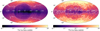 |
Fig. 10 Flux ratios of the Local Bubble (LB) all-sky maps (case 2a) and the Milky Way (MW) model for the 26Al (left) and 60Fe lines. The solid (dashed) lines show the regions where the Local Bubble is at least 1.0 (0.1) as strong as the Milky Way. The typical values for when the Local Bubble contribution might be stronger than the Galactic background shown here for 26Al and 60Fe are |b| ≳ 73° and |b| ≳ 48°, respectively. |
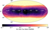 |
Fig. 11 Same as Fig. 10 but for the 511 keV line in case 1. The figure appears similar for case 2. For latitudes |b| ≳ 36°, the Local Bubble would dominate the Milky Way background as the flux ratio between the components is larger than 1. |
5 Expectations for COSI-SMEX
The Compton Spectrometer and Imager (COSI) is a small explorer (SMEX) mission planned for launch in 2027 (Tomsick et al. 2019, 2021, 2023). COSI-SMEX will be sensitive to soft γ-ray photons in the energy range between 0.2 and 5.0 MeV with a spectral resolution from 0.2–1.0% thanks to its Ge detectors. Due to its wide field of view of ~25% of the sky and its observation strategy that scans the whole sky within two of its low-Earth orbits, COSI-SMEX will be more sensitive to diffuse emission than any of its predecessors owing to the total grasp (effective area times field of view). The telescope will have an angular resolution on the degree scale which will make it suitable to detect a large number of point sources and extended emission such as from the Local Bubble. The satellite mission has a nominal duration of 2 yr for which we normalise the expectations in the following.
We use the latest mass model and corresponding response from COSI’s Data Challenge 2 (Karwin et al. 2022) to obtain exposure maps at the required γ-ray line energies from the dedicated COSI analysis software, cosipy (Martinez 2023). The instrumental background is provided by the COSI team (Gallego & Karwin, priv. comm.) and includes Earth albedo photons, atmospheric neutrons, primary alpha particles, electrons and positrons, primary and secondary protons, and an estimate of the Cosmic Gamma-ray Background (CGB). By multiplying our calculated model maps with the exposure maps in the respective bands and integrating over the whole sky, we can estimate the number of counts COSI-SMEX would receive per time. In Table 2, we list the expected rates for the different model assumptions detailed above.
For all three γ-ray lines considered here, two model assumptions of the Local Bubble (cases 1 and 2; LB 1 and LB 2 in Table 2), and an estimate of the Milky Way (MW), we calculate the count rate COSI-SMEX would receive per year, Ri, and the resulting total number of counts in its nominal 2 yr mission duration,  . From a simple consideration of the counts per time, we estimate the significance of each component against the Milky Way background only, or against the Milky Way background (γ-ray line plus diffuse Galactic continuum (cf. Sect. 4.4) plus the instrumental background. For simplicity, we assume that the images of the Galactic diffuse continuum roughly follow the γ-ray line images at their respective energies. It is clear from observations (e.g. Siegert et al. 2022a; Karwin et al. 2023) that the true spatial distribution from the Galactic diffuse continuum, mostly stemming from Inverse Compton scattering of electrons off the interstellar radiation fields, is not well determined but shows similarities to a normal galaxy with a bulge and a disk.
The significance is therefore calculated by
 (22)
(22)
where the unit of Si is the ‘number of sigmas’ scaled per time, that is,  , and can therefore easily be scaled by more or less exposure. We strongly emphasise that these estimates are bound to uncertainties because Eq. (22) is not strictly applicable, and, especially for small count rates (small significances), wrong (cf. Li & Ma 1983; Vianello 2018). A proper estimate would require a complete simulation of all components and a maximum likelihood analysis to ensure the reliability of such significance estimates. This is beyond the purpose of this study and we refer to Table 2 with caution.
The expected all-sky fluxes of the three γ-ray lines have a strong model dependence (see Table 1): The geometric model, case 1, typically shows smaller values for nuclear lines of26 Al and 60Fe, but a larger value for the 511 keV line from positron annihilation. While case 1 is a simple geometric model with heuristic assumptions, case 2 is a detailed hydrodynamics model to match ocean crust measurements, among others. We therefore created a reasonable bracket for further discussions (Sect. 6). Taking the fluxes at face value, we find that all three lines from the Local Bubble are within reach for COSI-SMEX, either within its nominal mission duration of 2 yr (most optimistic case), or within some additional years of observations. In particular, the 1809 keV line from the Local Bubble may reach a significance of 5σ above the Milky Way and instrumental background within ~4 yr – a 3σ hint may even be possible in 2 yr for the least optimistic case. The 60Fe lines may, in fact, be easier to detect as the fluxes are typically expected to be larger than the 26Al line. We note that the instrumental background around the 60Fe lines is typically larger, with chances of radioactive build-up on the timescale of years (Diehl et al. 2018; Siegert et al. 2019). In addition will the 60Fe lines sit on a much stronger diffuse γ-ray continuum compared to the 26Al line (Wang et al. 2020), which will probably lower the significance estimates in the case of 60Fe. The lines at 1332 and 1173 keV (same branching ratio) may be detected as almost-isotropic contribution within the first two years of COSI-SMEX. For positron annihilation, the model expectations of case 1 and 2 differ by a factor of ~11, making it either easy to detect such an isotropic contribution within one year, or very difficult to see an isotropic contribution at all from the Local Bubble. We note that the true emission morphology of positron annihilation from only the Local Bubble may be difficult to disentangle as positrons from other sources, also in addition to 26Al, may propagate into the Local Bubble and annihilate in its walls.
Expectations for COSI-SMEX.
6 Discussion
6.1 Systematic uncertainties
The calculated flux values for the three γ-ray lines at 1809, 1332, and 511 keV from the Local Bubble (Table 1) are subject to uncertainties from the modelling assumptions in each case discussed above. We estimate the impact of different parameters for the two cases and three lines in the following.
6.1.1 Nuclear lines: 1809 and 1332keV
In case 1, the nuclear lines from26 Al and 60Fe decay obtain their emissivities from geometrical and physical arguments, rather than hydrodynamics. This means that every parameter, including the ejecta masses, sound velocity inside the bubble, positions of the supernovae, order of spherical harmonics expansion of the bubble walls, uptake efficiency of 60Fe deposition on Earth, rotational velocity of the progenitors, and their metallicities, respectively, will change the appearance and total flux of the resulting images. From the stellar parameters alone, the uncertainty in the ejecta masses is within a factor of 10, which linearly impacts the total flux. In our above calculations, we used optimistic ejecta yields, but not the upper bounds, so that the the systematic uncertainties would be rather asymmetric with about 10% in the positive and 90% towards lower values. However, an extrapolation towards super-solar metallicities could lead to even higher radioactive ejecta masses. Comparing the yields and fluxes from case 1 to case 2 for the nuclear lines, the hydrodynamics simulations typically show a (much) larger present-day mass and therefore γ-ray line flux. These appear particularly large because instead of two, 13–14 supernovae contribute to the 26Al and 60Fe mass in the hydrodynamics simulation. Since the yields of these 13–14 supernovae are cumulating with time because the decay times of the radioisotopes are longer than the average delay time between successive supernovae (~0.7 Myr), there is more nuclear material present in the Local Bubble. This effect is particularly strong for 60Fe with a lifetime of 3.8 Myr and can readily explain the typical factors of ~10 difference in mass and flux between cases 1 and 2. The resulting fluxes from both cases can therefore be considered a bracket of systematic uncertainties for the 1809 and 1332 keV line. The isotropic contributions in both cases is similar, between 30–50% for the 1809 keV line and between 20–45% for the 1332keV line, which is also reassuring that the geometrical and physical considerations of case 1 are reasonable.
6.1.2 Positron annihilation line: 511 keV
In the case of positron annihilation, the systematics are similar to the nuclear lines: While the total amount of (not annihilated) positrons at any given time is directly given by the 26Al decay, Eqs. (16) and (19), that is, directly from the present mass of26 Al, it is unknown which part of the positrons annihilates when. The annihilation regions are determined in case 1 from the simple argument of diffusion being inefficient for low-energy positrons, even though they may propagate path lengths of several kpc. This means that the inner Local Bubble wall is the natural target, whose thickness can be estimated from weighing the diffusion time scale against the annihilation time scale, which results in thicknesses of ~10−3–100 pc. For case 1 we then assume that all positrons from 26Al some time ago (according to the cooling time) annihilate inside a 1 pc thick wall. From the uncertainty of the 26Al yields in case 1 alone, the total positron luminosity is uncertain by a factor of ~10, ranging from 1036–1037 e+ s−1. This directly impacts the 511 keV flux, then ranging from (2– 20) × 10−6 ph cm−2 s−1. The thickness of the walls also affects the measurable 511 keV flux: while thinner walls (in case 1) lead to the same flux, a distribution of the same number of positrons to thicker walls, for example 40 pc as could be expected from theory, the flux may decrease due to more positrons at larger distances. A similar argument can be considered for the 511 keV emission using the hydrodynamics simulation, case 2: here, the bubble walls are naturally about 20–30% of the thickness of the bubble radius, which distributes much of the positrons further out and decreases the flux. If then the bubble walls were thinner (assuming a larger boundary on the flow velocity), the flux may increase slightly by up to 10% when only the high luminosity regions in Fig. 6 would contribute. Other annihilation channels, such as radiative recombination and direct annihilation with non-zero kinetic energy, do not significantly contribute in the scenarios discussed here.
Two factors that may severely change the estimates here are the unsolved problem of propagation and the additional contribution from other positron sources. If the propagation of low-energy positrons is rather ballistic, the positrons that are created inside the Local Bubble (or anywhere in the Galaxy) will not annihilate in their close vicinity in the bubble walls or molecular clouds. This means that any isotropic contribution that we would measure at 511 keV would be the cumulative effect of all different sources whose propagated positrons will annihilate in our vicinity by chance. In such as case, the isotropic contribution to the 511 keV line may be even larger than what is discussed here. The additional positron sources are novae, pulsars, accreting compact objects, and possibly dark matter, among others (cf. Siegert 2023, for a recent review). All of them may be found inside the Local Bubble and their positron production rate will add to the predictions from 26Al alone and enhance the 511 keV flux. In summary, the 511 keV flux estimated from the Local Bubble should be found at least at a level of 2 × 10⁻⁶ ph cm−2 s−1, with large uncertainties to the upper end with optimistic values of (20–30) × 10−6 ph cm−2 s−1.
6.2 60Fe to 26Al ratio
For astronomical observations, the flux ratio of 60Fe to 26Al, r60/26, is of high importance because it gauges the stellar evolution models for massive stars. One has to distinguish between the mass ratio and the flux ratio of the two isotopes as they are only related by a numerical factor in a straightforward manner if and only if the distributions of 60Fe and 26Al are identical. We show in Fig. 12 that this is not the case. For both modelling assumptions, there is a certain contrast in the flux ratio maps which is the result of the different lifetimes of the isotopes again. This contrast is further enhanced in the simulations because 26Al is expelled by both winds of massive stars that live up to 0.88 Myr before present and their supernovae, whereas 60Fe is exclusively released by the supernovae, which leads to a slightly different geometry in case 1 and to more time available for mixing with the bubble walls in case 2. The γ-ray line map from 60Fe appears more homogeneous compared to 26Al because in the latter, the last supernovae can still be identified, owing also to the cumulative effect of the wind contributions which only occur for 26Al. The flux ratio, then, also depends strongly on the used yields and the number of supernovae responsible for the total mass and therefore flux. In case 1, the average flux ratio is about 0.32, whereas in case 2, it is 2.16. It should be noted that the individual hotspots in Fig. 12 (right, i.e. case 2) arise from turbulence which is not (or hardly) present in case 1. It can, however, increase the flux ratio to values beyond 10. Given the sensitivity of even COSI-SMEX, these pointed enhancements are probably too faint to be distinguishable and rather the average flux ratio will gauge the models. Clearly, the more supernovae there are that contribute, the higher the flux ratio, so that a measurement of the ratio, which is certainly within reach for COSI-SMEX (see Sect. 5), will reveal how many recent supernovae were responsible for the 60Fe anomalies measured on Earth (and the Moon). We note that the individual stellar evolution models themselves also have an impact on the resulting flux ratio, but that the large difference in our models originate purely in the number of super-novae exploded, so that one can distinguish certain scenarios by finding r60/26 larger or smaller than 1.0 as a rough guideline. This will also be in stark contrast to the Galactic-wide measurement of the flux ratio by Wang et al. (2020) of 0.18 ± 0.04stat, and up to 0.4 including systematic uncertainties.
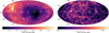 |
Fig. 12 Flux ratio per pixel of the 1332keV line from 60Fe versus the 1809keV line from 26Al. Left: case 1. Right: case 2. It is seen that the hot spots from 26Al in Fig. 7 are turned into cold spots in these flux ratio maps. The reason is again the 3.8 longer lifetime of 60Fe which lets the γ-ray emission of this isotope appear more homogeneous. We note the scales of the flux ratio maps: in case 1, the contrast is particularly small, whereas in case 2, the strong accumulation in of 60Fe already-mixed in the bubble walls increases the contrast up to a factor of 10. |
6.3 The Local Bubble viewed from the outside
The Local Bubble simulation by Schulreich et al. (2023) can be used as a surrogate model for (almost) any type of superbub-ble with an age of ~ 10–20 Myr. We place the hydrodynamics simulation at a distance of 200 pc from the Sun to perform line-of-sight integrations for 26Al, 60Fe, and positron annihilation, again, to inspect the appearance of a distant superbubble. For the same setup, the fluxes are 4.7 × 10⁻⁶, 14.5 × 10⁻⁶, and 2.6 × 10⁻⁶ ph cm−2 s−1 for the 1809, 1332, and 511 keV line, respectively. Certainly, these values are subject to the same systematic uncertainties, independent of the observer position.
We show the appearance of the three γ-ray lines viewed from the ‘outside’ in Fig. 13. The most intriguing factor here is that, again, 60Fe and26 Al are not co-spatial. This is important because this assumption is typically used in γ-ray data analyses, which require spatial templates. Here, the emission at 1809 keV appears more homogeneous with only slight enhancements from the turbulence, compared to the 1332 keV line with edge brightenings. The flux ratio, r60/26, is then identical to the case from observing inside the bubble, and would, if this was observed by a γ-ray telescope, gauge the age of the bubble by population synthesis (e.g. Siegert et al. 2023) rather than the number of supernovae that occurred. The positron annihilation map (Fig. 13, right) appears less structured with possible filaments due to annihilation in cold and dense clumps inside the superbubble as a result of thermal and hydrodynamic instabilities (possibly molecular clouds) and bubble walls. Again, the thickness is defined by the physical argument of where the transition region is from the bubble to the remaining interstellar medium of the Galaxy, not being neighboured by another bubble. Positron annihilation shows only a weak contrast as a function of bubble radius, which is surprising giving the fact that positrons only annihilate in dense regions. However, because of the thickness of the walls, the inho-mogeneities wash out and leave the 511 keV emission from a superbubble (at this age) as a distinct diffuse blob. It may well be the case that positrons diffuse through the bubble walls into other, neighbouring superbubbles (e.g. Orion-Eridanus), so that the annihilation flux of one superbubble cannot be estimated strictly by only assuming the 26Al ejecta masses. Many positron populations from different bubbles would probably add together in their boundaries.
7 Summary and outlook
In this work, we explain how we estimated the γ-ray line fluxes of the intermediate-lived radioactive isotopes 60Fe and26 Al, and the subsequent annihilation of positrons from the β+ decay of 26Al, in the Local Bubble. We based our estimates on two assumptions, one being a geometrical model that was derived to match the 3D dust extinction maps (Pelgrims et al. 2020), and one being a hydrodynamics simulation that was used to explain the deep-sea 60Fe deposits on Earth, among others (Schulreich et al. 2023). Despite these completely different approaches, the resulting fluxes for the 1809 keV line of 26Al, the two lines at 1173 and 1332 keV of 60Fe, and the positron annihilation line after the formation of Ps at 511 keV are consistent within an order of magnitude. The fluxes range from (3–20) × 10−6 ph cm−2 s−1 for26 Al, (4–10) × 10−6 ph cm−2 s−1 for 60Fe, and (2–20) × 10−6 ph cm−2 s−1 for positron annihilation. The fundamental difference in the assumptions is the number of supernovae within the last ~ 10 Myr that lead to the diffuse γ-ray flux now. While our geometrical model assumes only two supernovae, the hydrodynamics simulation assumes 13– 14 supernovae. This factor of 6–7 is directly reflected in the flux of the 1809 keV line, and leads to even larger differences in the case of 60Fe, up to a factor of 10. By measuring these fluxes inside the Local Bubble against the Milky Way background, one could further constrain models of the formation of the Local Bubble and the number of supernovae responsible for its current size and shape. In fact, with a 100-fold increase in sensitivity with respect to current telescopes (that is, INTEGRAL/SPI; Winkler et al. 2003; Vedrenne et al. 2003), one could even determine the direction of the last, that is, most recent, supernova in the Local Bubble.
While current γ-ray telescopes cannot measure these almost-isotropic signals, the future COSI-SMEX (Tomsick et al. 2023) satellite mission, slated for launch in 2027, will have a sensitivity that allows estimates of these γ-ray line fluxes. The time to reach a 5σ signal in the two nuclear lines varies between 0.1 and 4 yr against the instrumental background and the Milky Way background. We emphasise that these numbers should be considered with caution as the identification of large-scale signals is not trivial, and that the estimates for the instrumental background and exposure are subject to small changes until the launch. In addition, there will be contributions from the Galactic diffuse continuum (e.g. Siegert et al. 2022a) that will contribute to the line flux in small energy bands. Thanks to the excellent spectral resolution of COSI-SMEX, these contributions will be marginal in the case of 511 and 1809 keV, but can lead to a considerable bias in the case of the 60Fe lines at 1173 and 1332keV. If it is possible to determine the CGB (e.g. Inoue 2014) in the MeV range with COSI with high spectral resolution, one could compare the isotropic fractions of these lines attributed to the Local Bubble: We find that the ubiquitous contribution of the 26Al and 60Fe lines is between 20 and 50% of the total Local Bubble flux, thus also of the order of 10−6 ph cm−2 s−1.
The assumptions used in this study to estimate the 511 keV line flux from the26 Al decay in the Local Bubble walls results in either a very strong contribution of the order of 10−5 ph cm−2 s−1 with an isotropic contribution of 20–40% if based on our geometrical model, or rather weak fluxes around 10−6 ph cm−2 s−1 with a 10–15% isotropic contribution if based on the hydrodynamics simulation. The largest difference in our estimates probably results from the unknown propagation properties of low-energy positrons: While in the geometrical model, we find that, based on a uniform diffusion coefficient of 1028 cm2 s−1, all positrons naturally annihilate in the nearest 0.1–1.0 pc of the inner Local Bubble wall, and the hydrodynamics simulation provides 3D distributions of hydrogen densities and temperatures for the positrons to annihilate in with specific cross sections. We note that these are two extremely different assumptions, but which could be tested with a next generation telescope such as COSI.
By investigating the appearances of the 26Al and 60Fe maps of only the Local Bubble, the most important finding in this study is that the emission at 1809 keV and 1332 keV is not co-spatial. This is independent of the point of the observer and the modelling assumptions. If the Local Bubble is viewed from the ‘outside’, the 26Al emission at 1809 keV appears rather homogeneous with a slightly brighter central region compared to the outskirts with an indication of turbulence. In contrast, the 60Fe emission at 1173 and 1332keV is edge-brightened because the 60Fe had more time to mix with the denser hydrogen gas of the bubble wall until it started decaying with a 3.8 longer lifetime as 26Al. The wind contributions from 26Al furthermore led to a quasi-steady flow, which shapes the γ-ray image in a different way compared to 60Fe whose nucleosynthesis input is always explosive. In the context of γ-ray data analysis, which relies predominantly on spatial templates to determine the spectra and therefore fluxes of emission regions, the consensus is that assumptions on 26Al and 60Fe emission being co-spatial must be revised. If and only if the emission regions are identical can the flux ratios be converted into mass and production ratios and therefore inform us about stellar evolution models of massive stars.
 |
Fig. 13 Appearance of the γ-ray emission from the Local Bubble at 1809 keV (left), 1332keV (middle), and 511 keV (right) if it were to be observed from outside (here: 200 pc distance). It is evident that 26Al and 60Fe γ-ray emission is not co-spatial: the 1809 keV line appears more homogeneous with slight enhancements at the bubble walls compared to the 1332 keV line which shows an edge brightening. Positron annihilation only shows weak structures with bright spots from possible filaments. The thickness of the bubble wall is essentially determining the appearance of the 511 keV with only a weak contrast from inside the bubble towards the bubble walls. |
Acknowledgements
Saurabh Mittal and Hiroki Yoneda acknowledge support by the Bundesministerium für Wirtschaft und Energie via the Deutsches Zentrum für Luft- und Raumfahrt (DLR) under contract number 50 OO 2219.
Appendix A Derivation of Eq.(14)
Starting from the steady state assumption of Eq. (11),
 (A.1)
(A.1)
the equation to solve is
![Mathematical equation: $\eqalign{ & 0 = 4\pi {D \over {\kappa r}}\left[ {{n^*}(r){r^2} - {n^*}(r + {\rm{d}}r){{(r + {\rm{d}}r)}^2}} \right] \cr & \,\,\,\,\, - 4\pi {r^2}\dot a(T){n_{\rm{H}}}(r){n^*}(r){\rm{d}}r. \cr} $](/articles/aa/full_html/2024/09/aa50310-24/aa50310-24-eq42.png) (A.2)
(A.2)
Expanding the terms gives
![Mathematical equation: $\eqalign{ & 0 = {D \over {\kappa r}}\left[ {{n^*}(r){r^2} - {n^*}(r + {\rm{d}}r){r^2} - 2r{n^*}(r + {\rm{d}}r){\rm{d}}r} \right. \cr & \,\,\,\,\,\,\left. { - {n^*}(r + {\rm{d}}r){\rm{d}}{r^2}} \right] - {r^2}\dot a(T){n_{\rm{H}}}(r){n^*}(r){\rm{d}}r, \cr} $](/articles/aa/full_html/2024/09/aa50310-24/aa50310-24-eq43.png) (A.3)
(A.3)
of which the last term in the parenthesis approaches zero. Collecting the terms with powers of r results in
![Mathematical equation: $\eqalign{ & 0 = {D \over \kappa }\left[ {{n^*}(r)r - {n^*}(r + {\rm{d}}r)r - 2{n^*}(r + {\rm{d}}r){\rm{d}}r} \right] \cr & \,\,\,\, - \dot a(T){n_{\rm{H}}}(r){n^*}(r){r^2}{\rm{d}}r. \cr} $](/articles/aa/full_html/2024/09/aa50310-24/aa50310-24-eq44.png) (A.4)
(A.4)
where a spatial derivative of n*(r) with respect to r can be identified, so that
![Mathematical equation: $\eqalign{ & 0 = {D \over \kappa }\left[ { - r{{{\rm{d}}{n^*}(r)} \over {{\rm{d}}r}}{\rm{d}}r - 2{n^*}(r + {\rm{d}}r){\rm{d}}r} \right] \cr & \,\,\,\,\, - \dot a(T){n_{\rm{H}}}(r){n^*}(r){r^2}{\rm{d}}r, \cr} $](/articles/aa/full_html/2024/09/aa50310-24/aa50310-24-eq45.png) (A.5)
(A.5)
which can be reduced to
 (A.6)
(A.6)
In the limit of a thin shell slice, dr → 0, the new differential equation reads
 (A.7)
(A.7)
By simple integration, we arrive at the solution
![Mathematical equation: ${n^*}(r) = n_0^*\exp \left\{ { - \int {\left[ {{2 \over r} + {{\kappa \dot a(T){n_{\rm{H}}}(r)} \over D}r} \right]} {\rm{d}}r} \right\},$](/articles/aa/full_html/2024/09/aa50310-24/aa50310-24-eq48.png) (A.8)
(A.8)
which is equivalent to Eq. (14).
References
- Barros, D. A., Lépine, J. R. D., & Dias, W. S. 2016, A&A, 593, A108 [NASA ADS] [CrossRef] [EDP Sciences] [Google Scholar]
- Bennett, M., & Bovy, J. 2018, MNRAS, 482, 1417 [Google Scholar]
- Breitschwerdt, D., Egger, R., Freyberg, M., Frisch, P., & Vallerga, J. 1996, Space Sci. Rev., 78, 183 [NASA ADS] [CrossRef] [Google Scholar]
- Brown, B. L., & Leventhal, M. 1987, ApJ, 319, 637 [CrossRef] [Google Scholar]
- Chaikin, E., Kaurov, A. A., Fields, B. D., & Correa, C. A. 2022, MNRAS, 512, 712 [NASA ADS] [CrossRef] [Google Scholar]
- Cheng, J. Y., Rockosi, C. M., Morrison, H. L., et al. 2012, ApJ, 746, 149 [NASA ADS] [CrossRef] [Google Scholar]
- Cordes, J. M., & Lazio, T. J. W. 2002, NE2001.I. A New Model for the Galactic Distribution of Free Electrons and its Fluctuations, [arXiv:astro-ph/0207156] [Google Scholar]
- Diehl, R., Halloin, H., Kretschmer, K., et al. 2006, Nature, 439, 45 [CrossRef] [PubMed] [Google Scholar]
- Diehl, R., Siegert, T., Greiner, J., et al. 2018, A&A, 611, A12 [NASA ADS] [CrossRef] [EDP Sciences] [Google Scholar]
- Ekström, S., Georgy, C., Eggenberger, P., et al. 2012, A&A, 537, A146 [Google Scholar]
- Fuchs, B., Breitschwerdt, D., de Avillez, M. A., Dettbarn, C., & Flynn, C. 2006, MNRAS, 373, 993 [NASA ADS] [CrossRef] [Google Scholar]
- Fujimoto, Y., Krumholz, M. R., & Tachibana, S. 2018, MNRAS, 480, 4025 [NASA ADS] [CrossRef] [Google Scholar]
- Glebocki, R., & Gnacinski, P. 2005, in 13th Cambridge Workshop on Cool Stars, Stellar Systems and the Sun, eds. F. Favata, G. A. J. Hussain, & B. Battrick, ESA Special Publication, 560, 571 [NASA ADS] [Google Scholar]
- Guessoum, N., Jean, P., & Gillard, W. 2005, A&A, 436, 171 [NASA ADS] [CrossRef] [EDP Sciences] [Google Scholar]
- Inoue, Y. 2014, Cosmic Gamma-ray Background Radiation, https://fermi.gsfc.nasa.gov/science/mtgs/symposia/2814/proceedings/ [Google Scholar]
- Jean, P., Gillard, W., Marcowith, A., & Ferrière, K. 2009, A&A, 508, 1099 [NASA ADS] [CrossRef] [EDP Sciences] [Google Scholar]
- Karwin, C., Boggs, S., Tomsick, J., et al. 2022, in AAS/High Energy Astrophysics Division, 54, 108.30 [Google Scholar]
- Karwin, C. M., Siegert, T., Beechert, J., et al. 2023, ApJ, 959, 90 [CrossRef] [Google Scholar]
- Knödlseder, J. 1999, ApJ, 510, 915 [CrossRef] [Google Scholar]
- Knoedlseder, J., Dixon, D., Bennett, K., et al. 1999, A&A, 345, 813 [NASA ADS] [Google Scholar]
- Knoedlseder, J., Jean, P., Lonjou, V., et al. 2005, A&A, 441, 513 [NASA ADS] [CrossRef] [EDP Sciences] [Google Scholar]
- Krause, M. G. H., & Diehl, R. 2014, ApJ, 794, L21 [NASA ADS] [CrossRef] [Google Scholar]
- Krause, M., Fierlinger, K., Diehl, R., et al. 2013, A&A, 550, A49 [NASA ADS] [CrossRef] [EDP Sciences] [Google Scholar]
- Krause, M. G. H., Rodgers-Lee, D., Dale, J. E., Diehl, R., & Kobayashi, C. 2021, MNRAS, 501, 210 [Google Scholar]
- Kroupa, P. 2001, MNRAS, 322, 231 [NASA ADS] [CrossRef] [Google Scholar]
- Lallement, R., Vergely, J.-L., Valette, B., et al. 2014, A&A, 561, A91 [NASA ADS] [CrossRef] [EDP Sciences] [Google Scholar]
- Lallement, R., Babusiaux, C., Vergely, J. L., et al. 2019, A&A, 625, A135 [NASA ADS] [CrossRef] [EDP Sciences] [Google Scholar]
- Li, T.-P., & Ma, Y.-Q. 1983, ApJ, 272, 317 [Google Scholar]
- Limongi, M., & Chieffi, A. 2018, ApJS, 237, 13 [NASA ADS] [CrossRef] [Google Scholar]
- Luhman, K. L. 2022, AJ, 163, 24 [NASA ADS] [CrossRef] [Google Scholar]
- Martin, P., Strong, A. W., Jean, P., Alexis, A., & Diehl, R. 2012, A&A, 543, A3 [Google Scholar]
- Martinez, I. 2023, in Proceedings of 38th International Cosmic Ray Conference –PoS(ICRC2023), 444 [Google Scholar]
- Ore, A., & Powell, J. L. 1949, Phys. Rev., 75, 1696 [NASA ADS] [CrossRef] [Google Scholar]
- Pelgrims, V., Ferrière, K., Boulanger, F., Lallement, R., & Montier, L. 2020, A&A, 636, A17 [EDP Sciences] [Google Scholar]
- Pleintinger, M. M. M., Siegert, T., Diehl, R., et al. 2019, A&A, 632, A73 [NASA ADS] [CrossRef] [EDP Sciences] [Google Scholar]
- Pleintinger, M. M. M., Diehl, R., Siegert, T., Greiner, J., & Krause, M. G. H. 2023, A&A, 672, A53 [NASA ADS] [CrossRef] [EDP Sciences] [Google Scholar]
- Rodgers-Lee, D., Krause, M. G. H., Dale, J., & Diehl, R. 2019, MNRAS, 490, 1894 [NASA ADS] [CrossRef] [Google Scholar]
- Schulreich, M. M. 2015, PhD Thesis, Technische Universität Berlin, Germany [Google Scholar]
- Schulreich, M. M., Feige, J., & Breitschwerdt, D. 2023, A&A, 680, A39 [NASA ADS] [CrossRef] [EDP Sciences] [Google Scholar]
- Siegert, T. 2017, PhD Thesis, Technical University of Munich, Germany, https://mediatum.ub.tum.de/node?id=1340342 [Google Scholar]
- Siegert, T. 2023, Astrophys. Space Sci., 368, 27 [NASA ADS] [CrossRef] [Google Scholar]
- Siegert, T., Diehl, R., Khachatryan, G., et al. 2016, A&A, 586, A84 [NASA ADS] [CrossRef] [EDP Sciences] [Google Scholar]
- Siegert, T., Diehl, R., Weinberger, C., et al. 2019, A&A, 626, A73 [NASA ADS] [CrossRef] [EDP Sciences] [Google Scholar]
- Siegert, T., Berteaud, J., Calore, F., Serpico, P. D., & Weinberger, C. 2022a, A&A, 660, A130 [NASA ADS] [CrossRef] [EDP Sciences] [Google Scholar]
- Siegert, T., Horan, D., & Kanbach, G. 2022b, Telescope Concepts in Gamma-Ray Astronomy (Springer Nature Singapore), 1 [Google Scholar]
- Siegert, T., Pleintinger, M. M. M., Diehl, R., et al. 2023, A&A, 672, A54 [NASA ADS] [CrossRef] [EDP Sciences] [Google Scholar]
- Skinner, G., Diehl, R., Zhang, X., Bouchet, L., & Jean, P. 2014, in Proceedings of the 10th INTEGRAL Workshop: “A Synergistic View of the High-Energy Sky” (INTEGRAL 2014), 15–19 September 2014, Annapolis, MD, USA, online at http://pos.sissa.it/cgi-bin/reader/conf.cgi?confid=228, 054, 054 [Google Scholar]
- Snowden, S. L., Chiao, M., Collier, M. R., et al. 2014, ApJ, 791, L14 [NASA ADS] [CrossRef] [Google Scholar]
- Tomsick, J. A., Zoglauer, A., Sleator, C., et al. 2019, BAAS, 51, 98 [Google Scholar]
- Tomsick, J., Boggs, S., Zoglauer, A., et al. 2021, Am. Astron. Soc. Meeting Abstr. 53, 315.01 [Google Scholar]
- Tomsick, J., Boggs, S., Zoglauer, A., et al. 2023, in Proceedings of 38th International Cosmic Ray Conference – PoS(ICRC2023), 444 [Google Scholar]
- Vasini, A., Matteucci, F., & Spitoni, E. 2022, MNRAS, 517, 4256 [NASA ADS] [CrossRef] [Google Scholar]
- Vedrenne, G., Roques, J. P., Schönfelder, V., et al. 2003, A&A, 411, L63 [NASA ADS] [CrossRef] [EDP Sciences] [Google Scholar]
- Vianello, G. 2018, ApJS, 236, 17 [NASA ADS] [CrossRef] [Google Scholar]
- Wallner, A., Feige, J., Kinoshita, N., et al. 2016, Nature, 532, 69 [NASA ADS] [CrossRef] [Google Scholar]
- Wallner, A., Froehlich, M. B., Hotchkis, M. A. C., et al. 2021, Science, 372, 742 [NASA ADS] [CrossRef] [PubMed] [Google Scholar]
- Wang, W., Harris, M. J., Diehl, R., et al. 2007, A&A, 469, 1005 [NASA ADS] [CrossRef] [EDP Sciences] [Google Scholar]
- Wang, W., Lang, M. G., Diehl, R., et al. 2009, A&A, 496, 713 [NASA ADS] [CrossRef] [EDP Sciences] [Google Scholar]
- Wang, W., Siegert, T., Dai, Z. G., et al. 2020, ApJ, 889, 169 [NASA ADS] [CrossRef] [Google Scholar]
- Wang, X., Clark, A. M., Ellis, J., et al. 2021, ApJ, 923, 219 [NASA ADS] [CrossRef] [Google Scholar]
- Winkler, C., Courvoisier, T. J. L., Di Cocco, G., et al. 2003, A&A, 411, L1 [NASA ADS] [CrossRef] [EDP Sciences] [Google Scholar]
- Zucker, C., Goodman, A. A., Alves, J., et al. 2022, Nature, 601, 334 [NASA ADS] [CrossRef] [Google Scholar]
While no γ-ray line is associated with the decay of 53Mn, there are two potentially detectable ones at 554.6 and 597.4 keV for 244Pu, stemming from the 240Np decay to 240Pu. However, since we currently always consider the Local Bubble in isolation, i.e. without all the other superbubbles flanking it, which could also have swept up pre-existing 244Pu, we do not consider it worthwhile to carry out 244Pu line-of-sight integrations in the context of this paper.
This effect is similar to ‘over-fitting’, which results in arbitrarily good fits but may lack a sound interpretation.
The conversion for the ortho-Ps flux would then be  .
.
All Tables
All Figures
|
Fig. 1 Inner boundaries of the geometrical Local Bubble model as derived by Pelgrims et al. (2020). Shown are two different granularities of the spherical harmomics decomposition with lmax = 6 (left) and lmax = 40 (right). |
| In the text | |
|
Fig. 2 Mass distributions in the Local Bubble. Left: mass distributions of hydrogen (black; left axis), and 26Al (red) and 60Fe (blue; both isotopes right axis) as a function of nH in the hydrodynamics simulation by Schulreich et al. (2023). Note that the right axis is scaled by 10−9 to the left axis to allow a visual comparison. Right: cumulative distribution of the hydrogen, 26Al and 60Fe masses from the left panel with maximum (total) masses of 3.5 × 10⁵ M⊙, 1.6 × 10⁻⁵ M⊙ and 4.9 × 10⁻⁴ M⊙, respectively. Only cells for which the flow speed is higher than 1 km s−1 are used to ensure that the static background medium is not considered as part of the Local Bubble. |
| In the text | |
|
Fig. 3 Slices at y = 0 pc through the Schulreich et al. (2023) simulation for the number densities of 26Al (left) and 60Fe (right). It is evident that 60Fe is mostly found along the bubble walls whereas26 Al has also a large contribution of mass in the bubble’s hot phase. The position of the Sun is marked with dashed grey lines at ɀ = 20.8 pc. |
| In the text | |
|
Fig. 4 Slices at y = 0 pc through the Schulreich et al. (2023) simulation for the neutral hydrogen number density (left) and the temperature (right). The gas outside the Local Bubble is shaped according to the Galactic plane density distribution, decreasing exponentially towards higher |ɀ|. Small clumps of higher-density gas inside the bubble are visible in both panels, for example around (x, ɀ) = (80, −20) pc. The hot gas is naturally correlated with thin phases of the ISM, and the bubble walls are at a temperature of 8000 K or below. The position of the Sun is marked with dashed grey lines at ɀ = 20.8 pc. |
| In the text | |
|
Fig. 5 Positron annihilation rates per target density for the processes relevant in this study. The values (solid lines) are taken from Guessoum et al. (2005) and were rebinned (steps) for the purpose of assigning rates in the hydrodynamics simulation by Schulreich et al. (2023). |
| In the text | |
|
Fig. 6 Annihilation luminosity expected in the simulation by Schulreich et al. (2023) from only the charge exchange annihilation channel. Shown is the cell-averaged total luminosity for a slice through y = 0 pc. Clearly, boundary of the supershell shows the highest luminosity, together with the clouds inside the bubble. We again use the condition that the flow velocity must be larger than 1 km s−1 to distinguish the bubble from the background medium (see also Fig. 2). |
| In the text | |
|
Fig. 7 Expected all-sky maps from the decay of 26Al at 1809 keV in the Local Bubble. Left: case 1a of the geometrical model with a total flux of 3.3 × 10⁻⁶ ph cm−2 s−1. Right: case 2a of the hydrodynamics simulation with a total flux of 19.5 × 10⁻⁶ ph cm−2 s−1. See text for discussion and details. |
| In the text | |
|
Fig. 8 Same as Fig.7 but for the γ-ray line at 1332keV from 60Fe. The total fluxes are 4.6 × 10⁻⁶ ph cm−2s−1 and 42.2 × 10⁻⁶ ph cm−2s−1, respectively. |
| In the text | |
|
Fig. 9 Same as Fig. 7 but for the positron flux. The conversion to 511 keV flux is a factor of 0.568 (see text). The total 511 keV line fluxes are then 21.4 × 10⁻⁶ ph cm−2 s−1 and 2.0 × 10⁻⁶ ph cm−2 s−1, respectively. |
| In the text | |
|
Fig. 10 Flux ratios of the Local Bubble (LB) all-sky maps (case 2a) and the Milky Way (MW) model for the 26Al (left) and 60Fe lines. The solid (dashed) lines show the regions where the Local Bubble is at least 1.0 (0.1) as strong as the Milky Way. The typical values for when the Local Bubble contribution might be stronger than the Galactic background shown here for 26Al and 60Fe are |b| ≳ 73° and |b| ≳ 48°, respectively. |
| In the text | |
|
Fig. 11 Same as Fig. 10 but for the 511 keV line in case 1. The figure appears similar for case 2. For latitudes |b| ≳ 36°, the Local Bubble would dominate the Milky Way background as the flux ratio between the components is larger than 1. |
| In the text | |
|
Fig. 12 Flux ratio per pixel of the 1332keV line from 60Fe versus the 1809keV line from 26Al. Left: case 1. Right: case 2. It is seen that the hot spots from 26Al in Fig. 7 are turned into cold spots in these flux ratio maps. The reason is again the 3.8 longer lifetime of 60Fe which lets the γ-ray emission of this isotope appear more homogeneous. We note the scales of the flux ratio maps: in case 1, the contrast is particularly small, whereas in case 2, the strong accumulation in of 60Fe already-mixed in the bubble walls increases the contrast up to a factor of 10. |
| In the text | |
|
Fig. 13 Appearance of the γ-ray emission from the Local Bubble at 1809 keV (left), 1332keV (middle), and 511 keV (right) if it were to be observed from outside (here: 200 pc distance). It is evident that 26Al and 60Fe γ-ray emission is not co-spatial: the 1809 keV line appears more homogeneous with slight enhancements at the bubble walls compared to the 1332 keV line which shows an edge brightening. Positron annihilation only shows weak structures with bright spots from possible filaments. The thickness of the bubble wall is essentially determining the appearance of the 511 keV with only a weak contrast from inside the bubble towards the bubble walls. |
| In the text | |
Current usage metrics show cumulative count of Article Views (full-text article views including HTML views, PDF and ePub downloads, according to the available data) and Abstracts Views on Vision4Press platform.
Data correspond to usage on the plateform after 2015. The current usage metrics is available 48-96 hours after online publication and is updated daily on week days.
Initial download of the metrics may take a while.