| Issue |
A&A
Volume 636, April 2020
|
|
|---|---|---|
| Article Number | A123 | |
| Number of page(s) | 9 | |
| Section | Stellar structure and evolution | |
| DOI | https://doi.org/10.1051/0004-6361/201935787 | |
| Published online | 29 April 2020 | |
Discovery of a complex spiral-shell structure around the oxygen-rich AGB star GX Monocerotis⋆
1
ESO, Karl-Schwarzschild-Str. 2, 85748 Garching bei München, Germany
e-mail: This email address is being protected from spambots. You need JavaScript enabled to view it.
2
Academia Sinica Institute of Astronomy & Astrophysics (ASIAA), 11F of Astronomy-Mathematics Building, AS/NTU No.1, Section 4, Roosevelt Road, Taipei 10617, Taiwan
3
Joint ALMA Observatory, Alonso de Cordova 3107, Vitacura, Santiago 763 0355, Chile
4
Korea Astronomy and Space Science Institute 776, Daedeokdae-ro, Yuseong-gu, Daejeon 34055, Republic of Korea
5
National Science Foundation, 2415 Eisenhower Ave., Alexandria, VA 22314, USA
6
Uppsala University, Department of Physics and Astronomy, Box 516, 75120 Uppsala, Sweden
Received:
26
April
2019
Accepted:
17
March
2020
Abstract
The circumstellar envelopes of asymptotic giant branch (AGB) stars exhibit a wide range of morphologies and chemical compositions that can be exploited to unravel their mass-loss history as well as binary status. Here, we present ALMA Band 6 observations centred upon the oxygen-rich, high mass-loss rate AGB star GX Mon. The resulting CO (2–1) map reveals an intricate, complex circumstellar spiral-arc structure consistent with hydrodynamical models for an AGB experiencing mass loss in a highly eccentric, close binary system with an orbital period of around 140 years. Several other transitions (including SiO, SiS, SO2, and CS) are detected in the data, however only the SO (5–4) map shows a similar – although much weaker – distribution as imaged for the CO.
Key words: astrochemistry / stars: AGB and post-AGB / stars: mass-loss / circumstellar matter / submillimeter: stars
This paper makes use of the following ALMA data: ADS/JAO.ALMA#2016.1.00652.S. ALMA is a partnership of ESO (representing its member states), NSF (USA) and NINS (Japan), together with NRC (Canada), MOST and ASIAA (Taiwan), and KASI (Republic of Korea), in cooperation with the Republic of Chile. The Joint ALMA Observatory is operated by ESO, AUI/NRAO and NAOJ.
© ESO 2020
1. Introduction
Asymptotic giant branch (AGB) stars are low- to intermediate-mass (∼0.8−8 M⊙) stars in the final stages of their evolution. They are made up of a C/O core surrounded by a convective envelope. This is enshrouded by a gaseous and dusty circumstellar envelope (CSE) with a rich chemistry characterised by the elemental carbon-to-oxygen abundance ratio. According to this ratio, AGB stars are divided into C-type (carbon-rich, C/O > 1), M-type (oxygen-rich, C/O < 1), or S-type (C/O ≈ 1).
Stellar evolution on the AGB is governed by heavy mass loss at rates between 10−8 on the lower AGB and 10−4 M⊙ yr−1 at the tip of the AGB branch. This mass loss is thought to be triggered by long period, high amplitude pulsations that extend the atmosphere, thereby cooling the material and initiating dust formation near the stellar surface. Radiation pressure onto the ensuing dust grains then drives the stellar wind. Thermal pulses dredge up material from inside the star, which can be carried out by the stellar wind to form shells of gas and dust and contribute to the chemical evolution of the CSE. This means that during their AGB lifetime, some of these stars can convert from an oxygen-rich to a carbon-rich chemistry. The material around the AGB star is eventually ejected, for a significant fraction of the AGB stars forming a planetary nebula (PN), and returned to the interstellar medium as the star joins the white dwarf cooling track.
A detailed reconstruction of the CSE can provide valuable insights on the evolutionary state and history of the star, as well as the dynamical processes taking place. Of particular interest here is the effect of binary interactions, which are thought to play a crucial role in forming the wide variety of shapes observed in PNe (e.g. De Marco 2009). Since binary companions of most AGB stars cannot be detected directly due to their relative faintness or because they are enshrouded by dust, their presence must instead be inferred from arcs, spirals, or bubbles detected in the circumstellar material.
Observational studies of the dust and gas shells surrounding AGB stars recently received a massive boost with the advent of ALMA, which provides the necessary sensitivity, spatial, and spectral resolution for a very detailed mapping of individual molecular transitions at millimetre and sub-millimetre wavelengths. The picture that emerges is one of a very complex CSE morphology that varies widely depending on the star. Spiral and/or shell structures have been imaged for several C-type AGBs with high mass-loss rates, such as AFGL 3068 (Kim et al. 2017), R Scl (Maercker et al. 2012, 2016), and CW Leo (Cernicharo et al. 2015; Decin et al. 2015; Guélin et al. 2018). These structures within the otherwise mostly spherical CSEs are commonly attributed to binary companions. On the other hand, M-types with low mass-loss rates may harbour rotating dust and gas discs as inferred, for example, for L2 Pup (Kervella et al. 2016; Homan et al. 2017) or R Dor (Homan et al. 2018a). Some oxygen-rich stars with intermediate or high mass-loss rates are surrounded by a structure of bubbles or arc-like patterns, for example, IK Tau (Decin et al. 2018), EP Aqr (Homan et al. 2018b), or Mira (Mayer et al. 2011; Ramstedt et al. 2014). Two extreme OH/IR stars were recently reported to show broken ring-spiral patterns (Decin et al. 2019). Finally, the S-type star W Aql shows an asymmetric double-arc pattern, tentatively attributed to a binary orbit with low eccentricity (Ramstedt et al. 2017).
In this paper, we target the oxygen-rich AGB star GX Mon, a Mira-type variable at an approximate distance of around 650 pc1 (we assumed an average of the values quoted by Karovicova et al. 2013; Danilovich et al. 2015) with a relatively high mass-loss rate of 8.5 × 10⁻⁶ M⊙ yr−1 and a systemic velocity of −9 km s−1 (Danilovich et al. 2015). The large (V-K) index of ∼11 indicates that there is a large amount of dust surrounding the star, and archival Hubble Space Telescope (HST) images reveal circumstellar material with a radius of around 10″. Its inner dust shell was observed with infrared interferometry by Karovicova et al. (2013), who found that the data could be explained in terms of an Al2O3 and a silicate dust shell with inner radii of around 2 and 5 photospheric radii (Rphot), respectively. More recently, Danilovich et al. (2017) detected several sulphur-bearing molecules (H2S, SiS, SO, and SO2) in the envelope of GX Mon using the Atacama Pathfinder Experiment (APEX). The ALMA observations presented here constitute the first millimetre images for this star.
2. Data acquisition and processing
Our ALMA Cycle 4 observations of GX Mon were primarily designed to image the distribution of 12CO (2–1) in the CSE. Using the full spectral capabilities of ALMA, we acquired the continuum emission and targeted other lines of interest as well. Data from three different arrays were combined: C40-6 (our extended 12-m configuration), C40-3 (compact 12-m configuration), and the 7-m Atacama Compact Array (ACA). In order to be able to effectively combine data covering different spatial scales from several array configurations, ALMA computes different on-source integration times for each array. For this project, the on-source times were 2994 s, 907 s, and 1210 s, for the extended 12-m, compact 12-m, and 7-m array, respectively, requiring just one execution for each array and yielding a total on-source time of 1.4 h. The spectral setup used in the ALMA Band 6 covers the 215.13−218.88 and 230.14−232.98 GHz frequency ranges, while the channel width was chosen to match a spectral velocity resolution of 0.6 km s−1 for the spectral window containing the 12CO (2−1) line and ∼1.3 km s−1 for the other spectral windows.
The data for the different arrays were independently calibrated using the ALMA Pipeline. For each execution, the observing sequence schedules first a bandpass calibration, followed by a flux measurement and then a loop sequence alternating between a phase calibrator and the science target. For our observations, the flux calibrators were J0750+1231, J0750+1231, and J0510+1800 for the 7-m, compact 12-m, and extended 12-m configurations, respectively. Since the calibrators employed are all quasars (and therefore variable), ALMA monitors their flux regularly. With this approach, the error achieved for the flux calibration is approximately 10%.
The delivered data packages from the ALMA quality assurance (QA) procedure contained image cubes for several of the spectral lines detected, processed separately for each of the array components. However, since ALMA currently does not deliver the combined image products from the different arrays, we created our own final multi-scale images manually using CASA. As a first step, we merged all the calibrated data from the extended and compact 12-m, and 7-m arrays in the visibility (uv) domain. No additional weighting was applied between the 12- and 7-m data, as this was adequately taken into account by the relative on-source times. All the images presented here were then produced using the TCLEAN algorithm in CASA. We settled on the use of a standard Briggs weighting scheme with a robust parameter of 0.5. This yields an angular resolution of ∼0.16″ (for the CO image), corresponding to a spatial resolution of ∼105 AU at the assumed distance of GX Mon. On the large scale side, the inclusion of the 7-m array data allows us to recover structures as large as 30″. This is sufficient for mapping the entire envelope of GX Mon, which in both the CO image at the systemic velocity and the HST image, is smaller than 20″ in diameter.
We searched the entire bandwidth covered for line transitions. For the more morphologically complex lines, the imaging was done interactively using a combination of manually constructed channel-by-channel masks and the automated TCLEAN masking facility. This yielded high-fidelity images with minimal artefacts. For molecular transitions that show only compact and/or non-complex emission, a single elliptical mask was used. This way, we obtained image cubes for all detected emission lines with a typical sensitivity of 1.0 mJy beam−1 per 1.3 km s−1, an angular resolution of 0.19 × 0.13″, and position angle PA = −69.4 deg (using the CO cube as a reference).
3. Observational results
The transitions detected in our ALMA data are summarised, together with their key properties, in Table 1. By far the most striking feature in the data is the intricate morphology of the circumstellar envelope as mapped by the 12CO (2–1) transition. We focus our analysis and discussion mainly on this transition, as well as SO (5–4), which – although much weaker – also shows an arc and/or ring-like structure. Images and line profiles for the other transitions detected in the data (including SiO, SiS, SO2, 13CS, 29SiS, and 34SO) are briefly presented for completeness.
Lines detected in the ALMA observations of GX Mon.
3.1. 12CO (2–1)
The CO channel maps for GX Mon shown in Fig. 1 constitute some of the most detailed sub-mm images so far obtained for an M-type AGB star. They reveal a very complex disrupted spiral-ring structure in a circumstellar envelope extending out to a radius of ∼6″, or 4000 AU from the star, the morphology of which varies quite significantly across the line width of ∼40 km s−1, with a line peak of 0.13 Jy beam−1. While the envelope is well centred around the star and has an overall spherically symmetric shape, the distribution of the material within the envelope is rather irregular and clumpy, forming a messy conglomeration of spirals, arcs, and ridge-like segments. This is most readily explained by the distortion of the circumstellar material due to the presence of a companion, as is explored in more detail in Sect. 4.
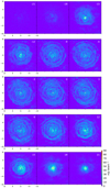 |
Fig. 1. Channel maps for the 12CO (2–1) emission. Images are shown for 1.3 km s−1 channel bins, spaced 3 km s−1 apart and shifted to zero at the systemic velocity of −9 km s−1. The overlaid white contours correspond to the SO emission, and trace 4, 5, 6, 10, and 14 times the rms value of 0.93 mJy beam−1. In this and all other spatial figures, the x and y axes give the relative RA and Dec in arcseconds from the position of GX Mon, unless otherwise indicated. |
Comparing our CO data to interferometric images presented for other AGB stars in the literature, we find some resemblance to the 12CO (3–2) transition observed in the OH/IR star OH 26.5 + 0.6 (Decin et al. 2019), an oxygen-rich star near the tip of the AGB with an extreme mass loss of up to 10−4 M⊙ yr−1. Scaling for distance, those data have a coarser angular resolution by a factor of two, so any smaller-scale or thinner arc structure may not be spatially resolved, but the basic clumpy, spiral-like morphology is recovered, and attributed to the effects of tidal interaction in a wide binary. The structure seen in GX Mon is also similar to the 12CO (2–1) distribution in the inner part of IRC+10216, the well-studied CSE of CW Leo (Cernicharo et al. 2015; Decin et al. 2015; Guélin et al. 2018). This is one of the nearest (∼130 pc) C-type thermally pulsing AGB stars characterised by a high mass-loss rate of ∼1.5 × 10⁻⁵ (De Beck et al. 2012) and a huge CSE extending out to 20 000 AU. Whereas the outer parts of the CSE consist of regularly spaced concentric rings, the inner ∼5000 AU shows a less well-organised structure of broken rings and arcs, similar to what we observe in GX Mon. The overall morphology of IRC+10216 could not be explained by the effects of a simple binary system, leading the authors to tentatively invoke a hugely variable mass-loss rate, or at least two companions.
3.2. SO (5–4)
Although much weaker than the CO at a peak line flux of 68 mJy beam−1, the SO (5–4) transition appears to show a similar morphology. While the central emission dominates by a factor of 3−4, there is evidence for an arc- or ring-like structure with a radius of 4−5″, as well as some material arranged in a broken arc morphology within about 2″ of the star (see left panel of Fig. 2). Interestingly, the presence of an SO ring was predicted for IK Tau, an oxygen-rich AGB star with a similar mass loss as GX Mon, based on a spectral survey of SO molecules (Danilovich et al. 2016), but to our knowledge, this is the first time that this has been imaged around an AGB star. In structure, it could be quite similar to the complex CN (2–1) thick ring detected around CW Leo (see Fig. 11 from Guélin et al. 2018), with the caveat that no central emission is detected for the latter. On the other hand, more sensitive data may reveal a spiral-like structure similar to the CO, extending all the way from the star to the outer edge of the CSE. The SO extended emission is very weak, and at the current sensitivity we are likely just seeing the tip of the iceberg.
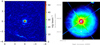 |
Fig. 2. Left: SO (5−4) line emission obtained by binning the velocity channels between −11.4 and −4.9 km s−1, chosen so as to emphasise the morphology of the weak ring and arc-like emission. Right: composite ACS/HST image of GX Mon in the F606W and F814W bands, overlaid with the SO (5–4) emission from the left panel (black contours). The white arrow indicates the direction of the proper motion as taken from Gaia DR2 via Simbad. |
An interesting peculiarity of the SO distribution is that – outside the central peak – the detected emission is strongest in a ridge-like feature around 5″ south/south-east of the star, peaking in intensity at velocities between –14 and –7 km s−1, that is, around the systemic velocity. While this ridge is not obviously associated with any particularly strong feature in the CO emission, it does have a clear counterpart in the visible Advanced Camera for Surveys (ACS)/HST archival image of GX Mon that we show in the right panel of Fig. 2. Although the area around the star is completely saturated in this image, there is evidence for circumstellar material organised in shells and/or arcs out to about 5″. The most prominent feature has an arc-like shape and perfectly coincides with the SO ridge from our ALMA data. Given that it lies in the direction of motion of the star (the Gaia proper motions are 0.093/−14.417 mas yr−1 in RA and Dec, respectively, and the resulting apparent direction of motion is indicated by the white arrow in Fig. 2), it is tempting to invoke a connection between the apparent build-up of material and the motion of the star with respect to the interstellar medium. However, since this ridge lies within rather than at the outer edge of the CSE as mapped by the CO, it is difficult to come up with a physically plausible explanation. It is quite possible that this apparent alignment is pure coincidence.
In order to better visualise the velocity structure of the SO emission, we show the channel-by-channel maps in Fig. 3. In addition to the spatial asymmetry already noted in Fig. 2, there appears to be an additional asymmetry in velocity space: the arc-like emission is strongest at positive velocities compared to systemic (especially between +6 and +12 km s−1), and all but disappears for negative velocities. Again, we find no convincing explanation for this asymmetry.
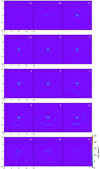 |
Fig. 3. Channel maps for SO (5–4). Images are shown for 1.3 km s−1 channel bins spaced 3 km s−1 apart and shifted to zero for the systemic velocity of −9 km s−1. |
A quick cross-check with the CO emission for those same velocity channels (see the contours in Fig. 1) reveals some overlap. In particular, the stronger SO emission in the +9 and +12 km s−1 channels compared to the systemic velocity coincides with a broadening in the CO arc-like structure. Comparing the position-velocity diagrams shown in Fig. 4, we can see that the SO structure matches that of the CO well, notably for outer arc extending out to 5″. This would indicate that the distribution of the two molecules is in fact very similar, although more sensitive maps are needed to fully appreciate the morphology of the SO.
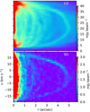 |
Fig. 4. Radial axis position-velocity diagram for the transitions of CO and SO. There is a clear correspondence between the CO ring-like structure at ∼5 arcsec and the outer SO ring. The colour scale has been chosen to bring up the weak emission of the SO transition. |
3.3. Other transitions and line profiles
We provide snapshot maps of the other transitions detected in Fig. 5. Looking at the strongest transitions SiO and SiS, we find that the v = 0 transition is spatially extended in both cases, reaching out to 1−2″ from the star, and exhibiting diffuse hints of an arc- or spiral-like structure. In contrast, the very strong v = 1 lines for both the SiO and SiS are spatially unresolved and attributed to maser emission near the stellar photosphere. The remaining transitions detected are relatively weak and/or unresolved, although there is a hint of some spatially extended structure for 29SiS and 34SO.
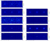 |
Fig. 5. Sample 1.3 km s−1 channel maps for the rest of the molecular lines detected towards GX Mon. Given the often narrower line widths compared to CO and SO, we show the velocity channels at −5, 0 and +5 km s−1 compared to the systemic velocity of −9 km s−1. See Table 1 for the full names of the transitions and the rest frequencies used. |
For completeness, we show the normalised, spatially integrated line profiles of all the transitions detected in Fig. 6. We note that in this plot, the rest frequency of the line in question was used to determine the velocity zero-point, and the resulting centre velocity of the lines is consistent with the systemic velocity of −9 km s−1 as taken from Danilovich et al. (2015). From looking at the line widths, it is apparent that the transitions can be divided into two main groups: broad lines with widths ∼40 km s−1 and narrow lines with widths ∼20 km s−1. The first category includes the spatially extended transitions CO, SO, SiO v = 0, SiS v = 0, 29SiS, and 34SO. Taking the data at face value, the very weak 13CS line also appears to fall in this category, while the SO2 is dominated by a strong central component and weaker broad wings. The second category encompasses the spatially unresolved SiO v = 1 and SiS v = 1, as well as the unknown transition. Interestingly, the SiO v = 1 line profile exhibits a split peak around the systemic velocity, which may point towards a rotation of the inner CSE. However, higher angular resolution data are required to confirm this.
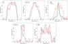 |
Fig. 6. Normalised spectra for all detected lines, separated in groups for better visualisation. The transitions are labelled with the corresponding colours. For the CO and SO lines, a circular region of 6″ in radius was used, encompassing the vast majority of the spatially extended emission. For the other more spatially compact molecules a box of 1.5 × 1.5″ was used. |
The continuum emission detected in the combined image, displayed in Fig. 7, is spatially unresolved, with an integrated flux of 9 mJy based on a 2D Gaussian fitting.
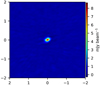 |
Fig. 7. Continuum image of GX Mon, revealing an unresolved, compact source at the centre. |
4. Discussion and comparison with models
As already mentioned, the prominent arc and spiral-like structure around GX Mon as traced in particular by the CO (2–1) emission is most likely caused by tidal interactions within a binary system. While such spirals around AGB stars have been modelled quantitatively for Carbon-rich stars (e.g. Kim et al. 2017; Maercker et al. 2012), the observed structure in those cases was a lot simpler, showing a relatively “clean” spiral. In contrast, the oxygen-rich GX Mon confronts us with a very messy, clumpy and irregular CSE morphology, which does not easily lend itself to interpretation.
The first step must therefore be to identify the main characteristics of the observed structure, before attempting any kind of comparison with models. For this, we focus on the systemic velocity channel of the CO, and find it instructive to construct an angle-radius diagram in Fig. 8. We used this plot to identify the following features by eye: (1) sloping diagonal lines corresponding (from bottom to top) to the first three windings of a spiral in RA, Dec space (white crosses); (2) a line with the opposite slope crossing the first winding (black crosses); (3) some noisy, wiggly structures on the second winding (yellow crosses); and a line with a steeper slope on the third winding (red crosses). Translating these markings into the spatial domain and over-plotting them onto a zoomed-in version of the CO distribution in Fig. 9, we obtain a schematic of the main features observed. These features include a clear spiral (white crosses), bifurcations of the main spiral structure (black and red crosses) as well as some wiggly deviations from the spiral shape (yellow crosses).
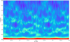 |
Fig. 8. Angle-radius diagram for the systemic velocity channel of the CO (2–1) transition observed for GX Mon. The main features identified by eye are marked with crosses (see text for details). Zero phase is defined as being west, with the phase running anti-clockwise. |
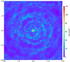 |
Fig. 9. Channel map for the systemic velocity of the CO emission, over-plotted with the main features identified from Fig. 8. |
A first comparison with the models recently published by Kim et al. (2019) reveals that the best compatibility of the features observed lies with the eccentric binary models computed by these authors. In particular, bifurcations of the spiral pattern are not predicted for circular orbits. A careful study of the central (close to the systemic velocity) panel of their Fig. 44, particularly the angle-radius diagram, reveals similar qualitative features as those identified for GX Mon: a bifurcation/discontinuity in the first winding, and noisy structure at approximately the same angular position in the second winding. The plot refers to Model 3, which adopts a binary eccentricity of 0.8, when viewed at a moderate inclination angle of i = 60°.
Encouraged by these findings, we constructed our own three-dimensional hydrodynamical simulations designed to be more representative of GX Mon, based on the same code as those presented by Kim et al. (2019). We invite the reader to refer to this publication as well as Kim & Taam (2012) and Kim et al. (2017) for details on the models as well as a discussion of the effects of the different model parameters on the simulation results. Our model uses the following parameters: mass of GX Mon M1 = 1 M⊙ (Justtanont et al. 1994), companion mass M2 = 1 M⊙ (assumption), orbital eccentricity e = 0.8 (assumption), average wind velocity of 22 km s−1 (from the spectral line width), orbital period Porb = 138 yr (determined by the pattern spacing in the CO emission image divided by the wind speed), radius of GX Mon R1 = 2.7 AU (Justtanont et al. 1994), and mass-loss rate Ṁ = 8.5 × 10⁻⁶ M⊙ yr−1 (Danilovich et al. 2015). The binary separation of the model is on average a = 34 AU (or about 10 stellar radii), varying from 7 AU at the pericentre to 61 AU at the apocentre (obtained by applying Kepler’s third law to the masses and orbital parameters above). We employed an adiabatic index γ = 1.4 and a computation domain size of 4000 AU, corresponding to ∼6″ at the assumed distance of 650 pc for GX Mon. After experimenting with several inclination angles, we found the best qualitative match to the CO map to occur for intermediate angles, and picked 45° for the illustrative purposes envisaged here.
The resulting model image for the systemic velocity is shown in Fig. 10. One can discern a clear spiral with some bifurcations, discontinuities, and noisier structure, the latter being due to the eccentricity introduced in the model. The spiral structure extracted from the observations is over-plotted and shows a good agreement with the model. Moreover, the bifurcations (black and red crosses) occur at a similar radial angle as in the model, and there is some overlap between the noisy structure observed (yellow crosses) and the part of the spiral affected by wiggles and splitting in the second winding. We note that the units of column density per projected velocity unit in the model image cannot be directly translated to the observed flux per beam on an absolute scale, and we limit our comparison to the relative structure seen in the two images.
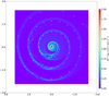 |
Fig. 10. Main structural components identified for GX Mon (crosses from Fig. 9) over-plotted on our representative model. |
Our results qualitatively demonstrate the consistency of the observed CO distribution with a close, highly eccentric binary system with an orbital period on the 150 year scale. The binary separation of course depends on the mass assumed for the companion, however not that sensitively. Varying M2 between 0.3 and 3 M⊙ gives a binary separation between 30 and 43 AU, which would make GX Mon one of the closest AGB star binaries found to date.
5. Conclusion
We uncovered a highly complex disrupted spiral-like structure in the CSE of the oxygen-rich AGB star GX Mon. While similar maps have been published for other high mass-loss AGB stars, this is one of the most intricate morphologies uncovered to date thanks to the sensitivity and high angular resolution of ALMA. The observed pattern is consistent with the density distribution simulated by the tidal interaction of a close binary companion on a highly eccentric orbit with the matter expelled from the AGB star. Although the observed morphology is too messy and noisy for a quantitative model fit, some features unique to an eccentric binary model, such as the tendency of the high-density arms to bifurcate are recovered. However, the greater complexity and tendency for the material to clump in the observed image suggests there may be additional factors at play that were not included in the model, such as variable mass loss, a third stellar component, or interactions of the CSE with the interstellar medium.
Interestingly, we find hints of a similar disrupted spiral pattern in the SO distribution, which seems to be concentrated in a ridge or arc in the direction of the motion of the star. Given that this ridge is located within the extent of the CO envelope it cannot constitute a bow shock, and we find no satisfying explanation for its apparent asymmetric distribution both in radial and velocity space. Unfortunately, the SO intensity is close to the detection limit in the current observations, therefore its real distribution is not well mapped. Clearly, more sensitive data are required to shed light on this enigmatic star.
While a Gaia parallax is available, such measurements are notoriously unreliable for stars with angular diameters on the same scale as the parallax measurement. The angular diameter of GX Mon is ∼8 mas compared to a measured parallax of 2.4251 ± 0.8645 mas (Gaia Collaboration 2018).
References
- Cernicharo, J., Marcelino, N., Agúndez, M., & Guélin, M. 2015, A&A, 575, A91 [NASA ADS] [CrossRef] [EDP Sciences] [Google Scholar]
- Danilovich, T., Teyssier, D., Justtanont, K., et al. 2015, A&A, 581, A60 [NASA ADS] [CrossRef] [EDP Sciences] [Google Scholar]
- Danilovich, T., De Beck, E., Black, J. H., Olofsson, H., & Justtanont, K. 2016, A&A, 588, A119 [NASA ADS] [CrossRef] [EDP Sciences] [Google Scholar]
- Danilovich, T., Van de Sande, M., De Beck, E., et al. 2017, A&A, 606, A124 [NASA ADS] [CrossRef] [EDP Sciences] [Google Scholar]
- De Beck, E., Lombaert, R., Agúndez, M., et al. 2012, A&A, 539, A108 [NASA ADS] [CrossRef] [EDP Sciences] [Google Scholar]
- De Marco, O. 2009, PASP, 121, 316 [NASA ADS] [CrossRef] [Google Scholar]
- Decin, L., Richards, A. M. S., Neufeld, D., et al. 2015, A&A, 574, A5 [NASA ADS] [CrossRef] [EDP Sciences] [Google Scholar]
- Decin, L., Richards, A. M. S., Danilovich, T., Homan, W., & Nuth, J. A. 2018, A&A, 615, A28 [NASA ADS] [CrossRef] [EDP Sciences] [Google Scholar]
- Decin, L., Homan, W., Danilovich, T., et al. 2019, Nat. Astron., 3, 408 [NASA ADS] [CrossRef] [Google Scholar]
- Gaia Collaboration 2018, VizieR Online Data Catalog: I/345 [Google Scholar]
- Guélin, M., Patel, N. A., Bremer, M., et al. 2018, A&A, 610, A4 [NASA ADS] [CrossRef] [EDP Sciences] [Google Scholar]
- Homan, W., Richards, A., Decin, L., et al. 2017, A&A, 601, A5 [NASA ADS] [CrossRef] [EDP Sciences] [Google Scholar]
- Homan, W., Danilovich, T., Decin, L., et al. 2018a, A&A, 614, A113 [NASA ADS] [CrossRef] [EDP Sciences] [Google Scholar]
- Homan, W., Richards, A., Decin, L., de Koter, A., & Kervella, P. 2018b, A&A, 616, A34 [NASA ADS] [CrossRef] [EDP Sciences] [Google Scholar]
- Justtanont, K., Skinner, C. J., & Tielens, A. G. G. M. 1994, ApJ, 435, 852 [NASA ADS] [CrossRef] [Google Scholar]
- Karovicova, I., Wittkowski, M., Ohnaka, K., et al. 2013, A&A, 560, A75 [NASA ADS] [CrossRef] [EDP Sciences] [Google Scholar]
- Kervella, P., Homan, W., Richards, A. M. S., et al. 2016, A&A, 596, A92 [NASA ADS] [CrossRef] [EDP Sciences] [Google Scholar]
- Kim, H., & Taam, R. E. 2012, ApJ, 759, 59 [NASA ADS] [CrossRef] [Google Scholar]
- Kim, H., Trejo, A., Liu, S.-Y., et al. 2017, Nat. Astron., 1, 0060 [NASA ADS] [CrossRef] [Google Scholar]
- Kim, H., Liu, S.-Y., & Taam, R. E. 2019, ApJS, 243, 35 [NASA ADS] [CrossRef] [Google Scholar]
- Maercker, M., Mohamed, S., Vlemmings, W. H. T., et al. 2012, Nature, 490, 232 [NASA ADS] [CrossRef] [PubMed] [Google Scholar]
- Maercker, M., Vlemmings, W. H. T., Brunner, M., et al. 2016, A&A, 586, A5 [NASA ADS] [CrossRef] [EDP Sciences] [Google Scholar]
- Mayer, A., Jorissen, A., Kerschbaum, F., et al. 2011, A&A, 531, L4 [NASA ADS] [CrossRef] [EDP Sciences] [Google Scholar]
- Ramstedt, S., Mohamed, S., Vlemmings, W. H. T., et al. 2014, A&A, 570, L14 [NASA ADS] [CrossRef] [EDP Sciences] [Google Scholar]
- Ramstedt, S., Mohamed, S., Vlemmings, W. H. T., et al. 2017, A&A, 605, A126 [NASA ADS] [CrossRef] [EDP Sciences] [Google Scholar]
All Tables
All Figures
|
Fig. 1. Channel maps for the 12CO (2–1) emission. Images are shown for 1.3 km s−1 channel bins, spaced 3 km s−1 apart and shifted to zero at the systemic velocity of −9 km s−1. The overlaid white contours correspond to the SO emission, and trace 4, 5, 6, 10, and 14 times the rms value of 0.93 mJy beam−1. In this and all other spatial figures, the x and y axes give the relative RA and Dec in arcseconds from the position of GX Mon, unless otherwise indicated. |
| In the text | |
|
Fig. 2. Left: SO (5−4) line emission obtained by binning the velocity channels between −11.4 and −4.9 km s−1, chosen so as to emphasise the morphology of the weak ring and arc-like emission. Right: composite ACS/HST image of GX Mon in the F606W and F814W bands, overlaid with the SO (5–4) emission from the left panel (black contours). The white arrow indicates the direction of the proper motion as taken from Gaia DR2 via Simbad. |
| In the text | |
|
Fig. 3. Channel maps for SO (5–4). Images are shown for 1.3 km s−1 channel bins spaced 3 km s−1 apart and shifted to zero for the systemic velocity of −9 km s−1. |
| In the text | |
|
Fig. 4. Radial axis position-velocity diagram for the transitions of CO and SO. There is a clear correspondence between the CO ring-like structure at ∼5 arcsec and the outer SO ring. The colour scale has been chosen to bring up the weak emission of the SO transition. |
| In the text | |
|
Fig. 5. Sample 1.3 km s−1 channel maps for the rest of the molecular lines detected towards GX Mon. Given the often narrower line widths compared to CO and SO, we show the velocity channels at −5, 0 and +5 km s−1 compared to the systemic velocity of −9 km s−1. See Table 1 for the full names of the transitions and the rest frequencies used. |
| In the text | |
|
Fig. 6. Normalised spectra for all detected lines, separated in groups for better visualisation. The transitions are labelled with the corresponding colours. For the CO and SO lines, a circular region of 6″ in radius was used, encompassing the vast majority of the spatially extended emission. For the other more spatially compact molecules a box of 1.5 × 1.5″ was used. |
| In the text | |
|
Fig. 7. Continuum image of GX Mon, revealing an unresolved, compact source at the centre. |
| In the text | |
|
Fig. 8. Angle-radius diagram for the systemic velocity channel of the CO (2–1) transition observed for GX Mon. The main features identified by eye are marked with crosses (see text for details). Zero phase is defined as being west, with the phase running anti-clockwise. |
| In the text | |
|
Fig. 9. Channel map for the systemic velocity of the CO emission, over-plotted with the main features identified from Fig. 8. |
| In the text | |
|
Fig. 10. Main structural components identified for GX Mon (crosses from Fig. 9) over-plotted on our representative model. |
| In the text | |
Current usage metrics show cumulative count of Article Views (full-text article views including HTML views, PDF and ePub downloads, according to the available data) and Abstracts Views on Vision4Press platform.
Data correspond to usage on the plateform after 2015. The current usage metrics is available 48-96 hours after online publication and is updated daily on week days.
Initial download of the metrics may take a while.