The ALMA-PILS survey: inventory of complex organic molecules towards IRAS 16293–2422 A

S. Manigand; J. K. Jørgensen; H. Calcutt; H. S. P. Müller; N. F. W. Ligterink; A. Coutens; M. N. Drozdovskaya; E. F. van Dishoeck; S. F. Wampfler

doi:10.1051/0004-6361/201936299

Home

All issues

Volume 635 (March 2020)

A&A, 635 (2020) A48

Full HTML

Free Access

Issue		A&A Volume 635, March 2020


Article Number		A48
Number of page(s)		30
Section		Interstellar and circumstellar matter
DOI		https://doi.org/10.1051/0004-6361/201936299
Published online		05 March 2020

A&A 635, A48 (2020)

The ALMA-PILS survey: inventory of complex organic molecules towards IRAS 16293–2422 A

S. Manigand¹, J. K. Jørgensen¹, H. Calcutt², H. S. P. Müller³, N. F. W. Ligterink⁴, A. Coutens⁵, M. N. Drozdovskaya⁴, E. F. van Dishoeck⁶^,7 and S. F. Wampfler⁴

¹ Niels Bohr Institute & Centre for Star and Planet Formation, University of Copenhagen, Øster Voldgade 5–7, 1350 Copenhagen K., Denmark
e-mail: sebastien@nbi.ku.dk
² Department of Space, Earth and Environment, Chalmers University of Technology, 41296 Gothenburg, Sweden
³ I. Physikalisches Institut, Universität zu Köln, Zülpicher Str. 77, 50937 Köln, Germany
⁴ Center for Space and Habitability (CSH), University of Bern, Gesellschaftsstrasse 6, 3012 Bern, Switzerland
⁵ Laboratoire d’Astrophysique de Bordeaux, Univ. Bordeaux, CNRS, B18N, allée Geoffroy Saint-Hilaire, 33615 Pessac, France
⁶ Leiden Observatory, Leiden University, PO Box 9513, 2300 RA Leiden, The Netherlands
⁷ Max-Planck Institut für Extraterrestrische Physik (MPE), Giessenbachstr. 1, 85748 Garching, Germany

Received: 12 July 2019
Accepted: 2 January 2020

Abstract

Context. Complex organic molecules are detected in many sources in the warm inner regions of envelopes surrounding deeply embedded protostars. Exactly how these species form remains an open question.

Aims. This study aims to constrain the formation of complex organic molecules through comparisons of their abundances towards the Class 0 protostellar binary IRAS 16293–2422.

Methods. We utilised observations from the ALMA Protostellar Interferometric Line Survey of IRAS 16293–2422. The species identification and the rotational temperature and column density estimation were derived by fitting the extracted spectra towards IRAS 16293–2422 A and IRAS 16293–2422 B with synthetic spectra. The majority of the work in this paper pertains to the analysis of IRAS 16293–2422 A for a comparison with the results from the other binary component, which have already been published.

Results. We detect 15 different complex species, as well as 16 isotopologues towards the most luminous companion protostar IRAS 16293–2422 A. Tentative detections of an additional 11 isotopologues are reported. We also searched for and report on the first detections of methoxymethanol (CH₃OCH₂OH) and trans-ethyl methyl ether (t-C₂H₅OCH₃) towards IRAS 16293–2422 B and the follow-up detection of deuterated isotopologues of acetaldehyde (CH₂DCHO and CH₃CDO). Twenty-four lines of doubly-deuterated methanol (CHD₂OH) are also identified.

Conclusions. The comparison between the two protostars of the binary system shows significant differences in abundance for some of the species, which are partially correlated to their spatial distribution. The spatial distribution is consistent with the sublimation temperature of the species; those with higher expected sublimation temperatures are located in the most compact region of the hot corino towards IRAS 16293–2422 A. This spatial differentiation is not resolved in IRAS 16293–2422 B and will require observations at a higher angular resolution. In parallel, the list of identified CHD₂OH lines shows the need of accurate spectroscopic data including their line strength.

Key words: astrochemistry / stars: formation / stars: protostars / ISM: molecules / ISM: individual objects: IRAS 16293–2422

© ESO 2020

1 Introduction

Complex organic molecules (COMs, i.e. molecules containing six or more atoms with at least one carbon atom; Herbst & van Dishoeck 2009) are observed in various interstellar environments, ranging from very cold, dense collapsing cloud cores (e.g. Bacmann et al. 2012; Taquet et al. 2017) to protoplanetary discs (e.g. Öberg et al. 2015; Walsh et al. 2016; Favre et al. 2018), as well as in low- and high-mass star-forming regions (e.g. Blake et al. 1987; Fayolle et al. 2015; Bergner et al. 2017; Ceccarelli et al. 2017; Ospina-Zamudio et al. 2018; Bøgelund et al. 2019). Meteorite measurements (Ehrenfreund et al. 2001; Botta & Bada 2002), comet coma observations (Bockelée-Morvan et al. 2000; Crovisier et al. 2004; Biver et al. 2014), and in situ Rosetta mission measurements (Le Roy et al. 2015; Altwegg et al. 2017) have revealed complex organic molecules, such as glycolaldehyde (CH₂OHCHO), ethylene glycol ((CH₂OH)₂), and glycine. The presence of complex and even pre-biotic species suggests that some of these molecules that formed during the earliest stage of stellar formation are preserved until the formation of small bodies. The extent to which the most complex species were formed at the earliest evolutionary stage of the protosolar nebula and how they were preserved or transformed during the formation of planetesimals remain open and complex questions.

In this study, we focus on the formation of COMs during the deeply embedded Class 0 stage. Class 0 protostars are characterised by an envelope that is rich in diverse molecules, where most of the mass of the system is gathered (Andre & Montmerle 1994). COMs may be observed in the inner regions of the envelope, which is close to their host protostar, where the temperature exceeds the water ice desorption temperature of ~100 K. These molecule-rich regions are called hot cores for high-mass protostars and hot corinos for low-mass counterparts. At sub-millimetre wavelengths, most of the lines originate from complex species. The measured COM abundances are typically between 10⁻⁷ and 10⁻¹¹ with respect to H₂ (e.g. Herbst & van Dishoeck 2009). In general, the formation of COMs is thought to occur on ice surfaces through a succession of different processes that are initiated by efficient hydrogenation of simple ice species, for example, CO, which leads to the efficient production of methanol (CH₃ OH; Garrod & Herbst 2006; Garrod et al. 2008; Fuchs et al. 2009; Chuang et al. 2018). During the collapse of the pre-stellar core, the temperaturestarts to increase during the so-called warm-up phase, and more complex species form and desorb into the gas phase in the hot corino. The resulting abundances of these species in the gas depend on the initial abundances of the precursors in the parent cloud, but they are also very sensitive to the physical conditions of the pre-stellar and protostellar phases and may thus vary significantly for different protostellar sources (Garrod 2013; Drozdovskaya et al. 2016). While the gas-phase formation pathways were not efficient enough to explain such high abundances of the COMs observed in the densewarm envelope, the recent progress in quantum chemical modelling brought attention back to the gas-phase chemistry (e.g. Balucani et al. 2015; Skouteris et al. 2018, 2019). Similar progress has been made recently in the study of the deuteration of COMs through gas-phase reactions (Skouteris et al. 2017). Careful comparisonsbetween observations and predictions from grain surface and gas-phase reaction experiments and calculations are needed to address the relative importance for the species that are present in their different protostellar environments.

Close protostellar multiple sources, that is, systems with multiple components separated by ≲ 1000 au, are particularly interesting laboratories for studying the effect of the physical conditions with time. Indeed, the chemical evolution of such sources is expected to stem from the same initial compositions and physical conditions (gas and dust temperatures as well as ultra-violet irradiation), which are inherited from the common parental cloud. The Class 0 low-mass protostellar binary IRAS 16293–2422 (IRAS 16293 hereafter), which is located in the ρ Ophiuchus cloud complex at a distance of ~140 pc (Dzib et al. 2018), is one of the best sources to investigate for that purpose. The components of the protostellar binary are known to be rich in COMs with abundances that are compara- ble to those seen towards high-mass protostars (van Dishoeck et al. 1995; Cazaux et al. 2003; Caux et al. 2011). Previous interferometric observations revealed abundance differences of specific molecules between the two protostars (Bisschop et al. 2008; Jørgensen et al. 2011, 2012); however, the origin of the differentiation is still debated. The Atacama Large Millimetre/ submillimetre Array (ALMA) Protostellar Interferometric Line Survey¹ (PILS, Jørgensen et al. 2016) performed an unbiased spectral survey of the system in Band 7, demonstrating the strength of ALMA for detecting new complex species towards the most compact component IRAS 16293 B of the system, including CH₃ Cl (Fayolle et al. 2017), CH₃ NC (Calcutt et al. 2018a), HONO (Coutens et al. 2019), NH₂CN (Coutens et al. 2018), and CH₃NCO (Ligterink et al. 2017). In addition, many deuterated and less abundant isotopologues have been found for the first time in the interstellar medium (ISM) towards this source, including NHDCHO, NH₂ CDO (Coutens et al. 2016), NHDCN (Coutens et al. 2018), CHD₂CN (Calcutt et al. 2018b), deuterated and ¹³C isotopologues of CH₂OHCHO, deuterated ethanol (C₂ H₅OH), ketene (CH₂CO), acetaldehyde (CH₃ CHO) and formic acid (HCOOH; Jørgensen et al. 2016, 2018), OC³³S (Drozdovskaya et al. 2018), and doubly deuterated methyl formate (CHD₂OCHO; Manigand et al. 2019). This paper aims to study the O-bearing COMs in the other protostar IRAS 16293 A of the binary system and to compare their abundances with IRAS 16293 B. Because of the proximity of the two sources (5″; ~720 au), the two sources are expected to have the same molecular heritage as their parent cloud. Therefore, any abundance difference between the sources could reveal the chemistry that occurred during the earliest evolutionary phases of this low-mass protostellar binary.

Similar comparative studies have been carried out towards the Class 0 binary protostar NGC 1333 IRAS 4A. López-Sepulcre et al. (2017) observed this source at high angular resolution with ALMA and measured the abundances of eight COMs towards the two components of the binary. The authors notice a large difference in abundance for all the species and suggest that the lack of COMs towards one of the source could be due to a lower mass, with a lower accretion rate, compared to the molecule rich counterpart.This scenario could alternatively suggest that the COM-poor source is not yet in the collapse phase resulting in the formation of the hot corino, which is consistent with the lack of evidence for the presence of a hot corino in this component (Persson et al. 2012). In contrast, both components in IRAS 16293 are known to harbour hot corinos.

In this study, we present an analysis of the PILS data taken towards IRAS 16293 A, which focus on the content of the O-bearing molecules in the hot corino region. This work aims to compare the abundances found for both components of the binary system to better understand the structure and/or the chemistry of this particular binary source. This paper is organised as follows. In Sect. 2, we describe the observations and spectroscopic data used in this study. In Sect. 3, we present the results of the observations and analyse the spectrum. In Sect. 4, we compare the abundances with those in IRAS 16293 B and discuss the different aspects of the two sources.Finally, we summarise the key points of the analysis and the discussion in Sect. 5.

2 Data analysis

In this section, we present the results of the oxygen-bearing COMs identification using the local thermodynamic equilibrium (LTE) analysis. In Sect. 2.1 we present the observations used in this study and the species identification is described in Sect. 2.2. The LTE model and the χ² -fitting are detailed in Sects. 2.3 and 2.4, respectively. Finally, the treatment of the uncertainties and the continuum correction are addressed in Sect. 2.5.

2.1 Observations

We used ALMA data from the PILS survey of the low-mass protostellar binary IRAS 16293 (Jørgensen et al. 2016). The data are a combination of the 12 m dishes and the Atacama Compact Array (ACA). The observations cover the frequency range of 329.1–362.9 GHz with a spectral resolution of 0.244 MHz, corresponding to ~0.2 km s⁻¹, and a restoring beam of 0.′′ 5. The survey reaches a sensitivity of 4–5 mJy beam⁻¹ km s⁻¹ across the entire frequency range. The ALMA software suite CASA (McMullin et al. 2007) was used to reduce the data, except for the continuum subtraction, which was performed after the data reduction (for more details, see Jørgensen et al. 2016). The flux calibration across the spectral range is consistent with the 5% level. The spectroscopic data of all the species that are analysed in this paper are detailed in Appendix C as well as the vibrational correction factors used, in the case of rotational temperatures that are higher than 100 K.

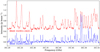Fig. 1

Portion of the spectrum towards IRAS 16293 A and IRAS 16293 B in red and blue, respectively, extracted on their corresponding offset positions. IRAS 16293 A spectrum is offset by 0.5 Jy beam⁻¹ for illustrative purposes.

2.2 Species identification

In this study, oxygen-bearing COMs have been investigated towards IRAS 16293 A and IRAS 16293 B through the analysis of the spectral emission at one position towards each source. The continuum peak positions, the strong continuum emission, the dynamics of the gas, and the spectral line density make it difficult to analyse the molecular emission. Therefore, the spectra were extracted towards offset positions at 0.′′6 from the continuum peak position in the north-east direction and 0.′′5 in the south-west direction for IRAS 16293 A and B, respectively. This is in agreement with the choice of the extracted spectrum position in the previous PILS studies (e.g. Calcutt et al. 2018b; Jørgensen et al. 2018; Lykke et al. 2017). Figure 1 shows the spectra towards IRAS 16293 A and B. Most of the lines identified towards IRAS 16293 B also appear in IRAS 16293 A, albeit at different intensities, which indicates that IRAS 16293 A is as rich in molecules as its companion. The line widths are typically two to threetimes larger towards IRAS 16293 A than towards IRAS 16293 B, thereby increasing the confusion due to blending effects.

The complexity of the molecular emission towards IRAS16293 A and B makes the line assignment to the species di- fficult whenbased on the peak frequency alone. In some cases, a species that was not considered to be present in the source might have a significant number of transitions with frequencies coinciding with bright transitions of other species. In order to deal with such line confusion, we coupled the identification of possible O-bearing COMs present in the gas to the LTE analysis. All the species detected in the counterpart protostar IRAS16293 B and their fainter isotopologues were considered as potential candidate species that compose the envelope of IRAS16293 A. Additionally, related and more complex O-bearing COMs have also been added to the list of candidates, such as trans-ethyl methyl ether (t-C₂ H₅OCH₃) and methoxymethanol (CH₃ OCH₂OH).

2.3 LTE model and detection criteria

We compared the extracted spectrum with a synthetic model in order to identify and derive the abundances of species that are present in the gas. The model applies the radiative transfer equations to a homogeneous column of gas along the line of sight under the LTE assumption. Only the optically thin lines, which have a line opacity lower than 0.1, are considered in the comparison of the modelled spectrum. For each species, a single excitation temperature was assumed to describe the level populations, which we refer to as rotational temperature.

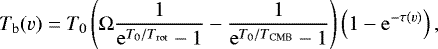
The brightness temperature T_b(v) depends on the line opacity τ(v), through the relation: $T_{b} (v) = T_{0} (Ω \frac{1}{e^{T_{0} / T_{rot}} - 1} - \frac{1}{e^{T_{0} / T_{CMB}} - 1}) (1 - e^{- τ (v)}),$ $\begin{equation*}T_{\mathrm{b}}(v) = T_{\mathrm{0}} \left(\Omega\frac{1}{\mathrm{e}^{T_{\mathrm{0}}/T_{\mathrm{rot}}}-1} - \frac{1}{\mathrm{e}^{T_{\mathrm{0}}/T_{\mathrm{CMB}}}-1} \right) \left(1-\mathrm{e}^{-\tau(v)} \right), \end{equation*}$ (1)

with T₀ = hν∕k_B, T_rot, the rotational temperature of the gas and the cosmic microwave background temperature T_CMB = 2.73 K. The filling factors of the gas emission, Ω, is equal to 0.5 (Jørgensen et al. 2016), corresponding to a source size of 0.′′ 5. The source size is the same as what was used in the previous studies of IRAS 16293 B based on the same dataset.

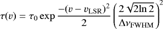
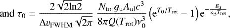
Under the LTE assumption and assuming a Gaussian profile, the line opacity is expressed as: $τ (v) = τ_{0} \exp \frac{- {(v - v_{LSR})}^{2}}{2} {(\frac{2 \sqrt{2 ln 2}}{Δ ν_{FWHM}})}^{2}$ $\begin{equation*} \tau(v) = \tau_{\mathrm{0}} \exp{\frac{-(v - v_{\mathrm{LSR}})^2}{2}\left(\frac{2\sqrt{2\mathrm{ln}\,2}}{\Delta\nu_{\mathrm{FWHM}}}\right)^2} \end{equation*}$ (2) $and τ_{0} = \frac{2 \sqrt{2 ln 2}}{Δ v_{FWHM} \sqrt{2 π}} \frac{N_{tot} g_{u} A_{ul} c^{3}}{8 π Q (T_{rot}) ν_{0}^{3}} (e^{T_{0} / T_{rot}} - 1) e^{- \frac{E_{u}}{k_{B} T_{rot}}},$ $\begin{equation*} \text{and } \tau_0 = \frac{2\sqrt{2\mathrm{ln}2}}{\Delta v_{\mathrm{FWHM}}\sqrt{2\mathrm{\pi}}} \ \frac{N_{\mathrm{tot}} g_{\mathrm{u}} A_{\mathrm{ul}} c^3}{8\mathrm{\pi} Q(T_{\mathrm{rot}}) \nu_{\mathrm{0}}^3} \left(\mathrm{e}^{T_{\mathrm{0}}/T_{\mathrm{rot}}} - 1\right) \mathrm{e}^{-\frac{E_{\mathrm{u}}}{\mathrm{k_B} T_{\mathrm{rot}}}}, \end{equation*}$ (3)

where g_u is the upper state degeneracy, E_u is the upper state energy, A_ul is the Einstein coefficient of the transition, N_tot is the column density, and Q(T_rot) is the partition function evaluated at T_rot. We note that the brightness temperature and the line opacity are functions of the velocity v, representing the velocity shift with respect to the peak velocity, v_LSR, which was set at the rest frequency of the modelled line. The parameters T_ex, N_tot, v_LSR and Δv_FWHM, the full line width at half-maximum in velocity units, are free parameters in the model.

The detection criteria for a species in the PILS data is mostly affected by the high density of the line present in the spectrum, which is more problematic towards IRAS16293 A due to the broader lines. A line is considered to be unblended, and thus usable for the fit, in the following cases: if there is no line from another species in the ν₀ ± 2FWHM frequency range (i.e. Rayleigh criteria); and if there is a line in the ν₀ ± 2FWHM frequency range but the peak intensity of this line is lower than 10% the peak intensity of the line of interest or less than 1σ.

The frequency range considered in the Rayleigh criteria is extended to ± 4FWHM at the proximity of a very optically thick blending line, for example, the low-E_up CH₃ OH lines.

2.4 χ²-fitting

Towards the analysed position, 0.′′ 6 north-east of IRAS 16293 A, a line width FWHM of 2.2–2.4 km s⁻¹, and a peak velocity v_lsr of 0.8 km s⁻¹ reproduce the emission line shapes of all the species in this study, suggesting that they are indeed located in the same region around the protostar. The line width and the peak velocity towards the offset position from IRAS 16293 B, which are 1.0 and 2.7 km s⁻¹, respectively,are consistent with the range of values from the previous PILS studies (0.8–1.0 km s⁻¹ and 2.5–2.7 km s⁻¹, respectively, Coutens et al. 2016; Lykke et al. 2017; Calcutt et al. 2018a; Persson et al. 2018; Ligterink et al. 2017).

The species that are considered have been fitted on a grid in column density and rotational temperature, ranging from 10¹⁴ to 10¹⁸ cm⁻² in logarithmic scale and from 75 to 300 K by increments of 5 K, respectively. Each of them were iteratively fitted from the most to least abundant and put in a reference spectrum that was taken into account for the fit of the next species.

The comparison between the observed spectrum and the model is quantified by the χ² minimisation, which is defined as $χ^{2} = \sum_{lines} \int_{line profile} ω (v) {(\frac{I_{b} (v) - T_{b} (v)}{σ_{b} (v)})}^{2} d v,$ $\begin{equation*}\chi^2 = \sum_{\text{lines}}{\int_{\text{line profile}} \omega(v)\left(\frac{I_{\text{b}}(v) - T_{\text{b}}(v)}{\sigma_{\text{b}}(v)}\right)^2 \text{d}v}, \end{equation*}$ (4)

where I_b(v) and σ_b (v) are the line intensity and the intensity uncertainty of the extracted spectrum, respectively. We note that the intensity uncertainty includes the contribution from the calibration uncertainty σ_cal, the root mean square (RMS) σ_RMS, and the following: $σ_{b} (v) = \sqrt{σ_{RMS}^{2} (v) + σ_{cal}^{2} (v)}$ $\sigma_{\text{b}}(v) = \sqrt{\sigma^2_{\text{RMS}}(v) + \sigma^2_{\text{cal}}(v)}$ .

The weighting factor ω(v) is equal to three if T_b(v) > I_b(v), and it is one otherwise. In the case of this study, this weighting factor provides a better constraint on possible blending effects, which could bias the minimisation. In other words, the weighting factor increases the χ² value when the model is above the spectrum. We chose to break the symmetry of the model that way to allow the fitting procedure to converge to lower column density values compared to those derived with a symmetric χ², which could include possible contributions from species that are close enough for blending. The choice of the weighting factor value of three is arbitrary and depends on the degree of line confusion in the data.

2.5 Uncertainties and continuum corrections

The uncertainties are usually given by the covariance matrix, which is estimated in the standard χ² minimisation methods. However, the modified χ² used in this study no longer allows for the use of the covariance matrix to get the uncertainties. Instead, the uncertainties have been estimated using a simple Monte Carlo simulation, where the spectrum as well as an additional Gaussian noise of σ_b (v) amplitude were fitted to the synthetic spectrum several times. This gives a distribution of each parameter; here, the excitation temperature and the column density are called the posterior probability distributions. This versatile method has also been successfully used to estimate the uncertainties on the 3 μm OH band model parameters as well as in reflectance spectroscopy of meteorites and asteroids (Potin et al. 2019). In summary, the posterior probability distribution of the parameters represents the distribution of the possible values that can take each parameter, given the uncertainties of the data. The formalism of this Monte Carlo simulation is detailed in Appendix B.

This statistical estimation of the uncertainties gives much lower relative errors on the excitation temperature and column density compared to the actual data relative uncertainties. This suggests that the proper statistical estimate of the errors is not conservativeconsidering the underlying hypotheses of the LTE model and how they are handled in the minimisation. Indeed, the χ² minimisation assumes that the model is perfect and determines the best set of parameters to fit the observations. However, the observationsinclude many effects that are neglected by the LTE analysis but which appear in the spectrum. These effects can be, for example, non-uniform source coverage, beam dilution, self-absorption effects, or abundance gradients of the species in the line of sight (with the associated velocity shift). Therefore, we chose to take conservative values of ~20 and ~30% for the rotational temperatures and the column densities relative uncertainties, respectively, for IRAS 16293 A. For consistency, the relative uncertainty values used in the study of Jørgensen et al. (2018) are assumed for IRAS 16293 B, that is, ~20 and ~10% for the rotational temperatures and the column densities, respectively.

The dust emission is treated as a continuum brightness temperature, which is directly derived from the continuum emission in the same frequency range. The high density of both sources makes it so the dust emission is partially coupled to the gas emission. In order to take into account the continuum contribution to the line emission, the correction factor A_corr was applied to the column density $A_{corr} = \frac{Ω \frac{1}{e^{T_{0} / T_{rot}} - 1} - \frac{1}{e^{T_{0} / T_{CMB}} - 1}}{Ω \frac{1}{e^{T_{0} / T_{rot}} - 1} - Ω_{dust} \frac{1}{e^{T_{0} / T_{d}} - 1}}$ $\begin{equation*} A_{\text{corr}} = \frac{\Omega\frac{1}{\mathrm{e}^{T_{\mathrm{0}}/T_{\mathrm{rot}}}-1} - \frac{1}{\mathrm{e}^{T_{\mathrm{0}}/T_{\mathrm{CMB}}}-1}}{\Omega\frac{1}{\mathrm{e}^{T_{\mathrm{0}}/T_{\mathrm{rot}}}-1} - \Omega_{\text{dust}}\frac{1}{\mathrm{e}^{T_{\mathrm{0}}/T_{\mathrm{d}}}-1}} \end{equation*}$ (5)

in which T_d is the dust brightness temperature and Ω_dust is the dust emission filling factor, which is assumed to be equal to Ω. Under the LTE assumption, the use of a correction factor is equivalent to replacing T_CMB with the dust brightness temperature T_d in Eq. (1). The dust brightness temperatures used in this paper are 30.1 and 21.2 K towards the offset position from continuum peak positions towards IRAS16293 A and B, respectively. The value of the continuum correction factor ranges from ~1.1 at 300 K to ~1.4 at 90 K and it does not strongly depend on the frequency across the spectral range of the PILS data.

3 Results

In total, 15 different species as well as 16 isotopologues, have been securely detected, while 11 additional species and isotopologues are tentatively identified towards IRAS 16293 A. Table 1 shows the result of the LTE analysis with the number of lines taken into account in the minimisation, the best-fit parameters (i.e. T_rot, N_tot, and Δv_FWHM), the abundance with respect to the main isotopologue for the same species, and the corresponding isotopic ratio.

3.1 Abundances and rotational temperatures

The relativeabundances of the oxygen species are determined from their column density relative to the column density of CH₃OH. We note that H₂ was not used as a reference for the estimation of the abundances because only the lower limit of H₂ column density can be determined from the optically thick dust emission. Calcutt et al. (2018b) and Jørgensen et al. (2016) estimated the lower limit of H₂ column density towards IRAS 16293 A and B, respectively. The D/H ratio is based on the column density ratio and is corrected from the statistics of H atoms in the deuterated chemical group of the molecule. For example, the column density ratio of CH₂DOH is three times higher than its D/H ratio. In addition, the statistical correction includes the symmetries in the sense of the rotational spectroscopy. For example, the asymmetric deuterated dimethyl ether (a-CH₂DOCH₃) has four possible sites where the D atom could be placed, that is, out of the C–O–C plane, regardless of the rotational emission of the molecule. Thus, its column density ratio is four times higher than the D/H ratio. Similarly, the symmetric s-CH₂DOCH₃ conformer has two in-plane possible sites for the D atom, which leads to a factor of two between the column density ratio and the D/H ratio. The rotational temperature of the isotopologues was fixed to the value derived for their main isotopologue, except for formaldehyde (H₂ CO) where only the H $_{2}^{13}$ $_2^{13}$ CO rotational temperature could be constrained. For several isotopologues, the fit converged to a different rotational temperature as the main isotopologue. The difference is lower than the uncertainty for the rotational temperature and does not significantly affect the column density. The results of the minimisation for these species are indicated in the notes of Table 1. Despite the large frequency range of the survey, H₂ CO isotopologues only have a few lines in the range, and most of them are either optically thick or the transition levels are not populated at all (E_up > 1000 K). The rotational temperature was derived using two optically thin lines of H $_{2}^{13}$ $_2^{13}$ CO, with upper state energies of 98 and 240 K. The optically thin lines, which were used to derive the column density of the other isotopologue, are the same lines used by Persson et al. (2018) in the analysis of IRAS 16293 B.

Similar to the study of IRAS 16293 B (Jørgensen et al. 2018), a large number of rarer isotopologues were also identified towards IRAS 16293 A. We note that CH $_{3}^{18}$ $_3^{18}$ OH and H₂ C¹⁸O show a ¹⁶O/¹⁸O ratio close to the local interstellar medium value of 557 ± 30 (Wilson 1999). The upper limit column density of H₂ C¹⁷O is consistent with the canonical ¹⁶O/¹⁷O ratio of 2005 ± 155 (Penzias 1981; Wilson 1999). The ¹³C-isotopologues that were detected do not show any significant deviation from the local ISM ¹² C/¹³C ratio of 68 ± 15 (Milam et al. 2005). Lower ¹²C/¹³C ratios have been reported towards IRAS 16293 B (Jørgensen et al. 2018) and were interpreted by a chemical process that is similar to the deuteration enhancement on the ice grain surface, which occurs during the pre-stellar formation stage. However, the mean ¹²C/¹³C ratio of 76 ± 12 towards IRAS 16293 A is consistent with the local ISM value, which indicates that the isotopic enhancement mechanism observed in IRAS 16293 B does not occur in IRAS 16293 A. Deuterated isotopologues of CH₃OH, H₂ CO, C₂ H₅OH, dimethyl ether (CH₃OCH₃), CH₃OCHO, CH₂CO, HCOOH, and isocyanic acid (HNCO) are present in the gas with D/H ratios of 2–5%. As it was observed towards IRAS 16293 B (Persson et al. 2018; Manigand et al. 2019), the doubly-deuterated isotopologues D₂ CO and CHD₂OCHO are significantly enhanced compared to the singly-deuterated isotopologues. The implications are discussed in the next section of the paper.

New spectroscopic data for deuterated CH₃CHO isotopologues were recently reported by Coudert et al. (2019) who add information about CH₂DCHO to that of CH₃CDO from Elkeurti et al. (2010), which was utilised for the first detection reported by Jørgensen et al. (2018). To test their experimental results, Coudert et al. (2019) used the new spectroscopic data to search for CH₂DCHO and CH₃CDO in the PILS dataset. They report the presence of 93 and 43 transitions of CH₂DCHO and CH₃CDO across a 10 GHz frequency range, respectively, and they made rough estimates of the column densities based on the archival 12 m array PILS data only. In order to carry out a consistent comparison of the PILS results in terms of assumptions concerning analysed positions, source sizes, velocity shift, and FWHM as well as using the combined 12m+ACA dataset, we analysed the data for those isotopologues with the same methodology in this paper as the other PILS papers. The derived column density and rotational temperature are reported in Table 2. The new column density reported for CH₃CDO is consistent with the value that was derived in the previous study of Jørgensen et al. (2018).

3.2 New detections

In addition to the 31 identified isotopologues towards IRAS 16293A, two new species, CH₃OCH₂OH and t-C₂ H₅OCH₃, were detected towards IRAS 16293 B, exclusively. Only an upper limit column density was derived for the two species towards IRAS 16293 A, assuming the same rotational temperature as for IRAS 16293 B. Column densities, relative abundances to CH₃OH, and upper limits are reported in Table 2. Both species have already been detected in the ISM before; however, this is the first time they were detected in a low mass star-forming region. McGuire et al. (2017) report the detection of CH₃OCH₂OH towards the high-mass protostellar core NGC 6334I MM1, with a relative abundance of ~0.03 with respect to CH₃OH. This abundance is significantly higher than those towards IRAS 16293 A and IRAS 16293 B and this is discussed in the next section along with the other O-bearing species. We note that t-C₂ H₅OCH₃ was tentatively detected in several high-mass sources, such as W51 e1/e2 (Fuchs et al. 2005), which was refuted by Carroll et al. (2015) and Orion KL (Tercero et al. 2015). Later, Tercero et al. (2018) confirmed the detection towards the Orion KL compact bridge region. The last study reported a rotational temperatureof 150 ± 20 K and a column density of 3.0 ± 0.9 × 10¹⁵ cm⁻², leading to an abundance of 3.7 × 10⁻⁹ with respectto H₂. This estimation is consistent with the abundance derived towards IRAS 16293 A and B.

3.3 Identification of CHD₂OH lines

Thirty-one lines of CHD₂OH were found in the range of the observations. CHD₂OH has already been detected at lower frequencies towards IRAS 16293 (Parise et al. 2002) using the IRAM 30-metre telescope. At the present day, only a small number of lines are publicly available in terms of spectroscopic data, including the line strength values, although, more extended frequency lists can be found in the literature (e.g. Ndao et al. 2016; Mukhopadhyay 2016). Therefore, this species requires special treatment.

To confirm the identification CHD₂OH in spectrum,each line was independently fitted to a simple Gaussian line profile in terms of amplitude and by using the same velocity peak v_lsr and FWHM as CH₃OH, that is, 0.8 and 2.2 km s⁻¹ as well as 2.7 and 1.0 km s⁻¹ for IRAS 16293 A and IRAS 16293 B, respectively. The line frequencies match 24 and 16 lines of the 31 candidates, for IRAS 16293 A and B, respectively, without any hint of blending effect with other species. Figures D.1 and D.2 show the Gaussian fits of all the lines. The integrated intensity over ± FWHM around the rest frequency was derived for each unblended lines and is noted in Table D.1. The average integrated intensity of the lines assigned to CHD₂OH is higher than 0.3 Jy beam⁻¹ km s⁻¹ for IRAS 16293 B. Also, several liness towards IRAS 16293 B show a small blue-shifted absorption counterpart, which is a characteristic of infalling motions (Pineda et al. 2012), which are associated with optically thick lines. In comparison to the other detected species, especially to CH₂DOH and CH₃OH, these intensities correspond to high line opacities due to a high column density. This suggests a high abundance of CHD₂OH as well, and it is a key factor motivating further searches for CD₃OH, as was already detected by Parise et al. (2004), and CD₃OD. Despite the substantial data available on CD₃OH and CD₃OD (Mollabashi et al. 1993; Walsh et al. 1998; Xu et al. 2004; Müller et al. 2006), we did not find any line that corresponds to those of these two species in the present observations.

Table 1

Best-fit results of all the detected and tentatively detected species towards IRAS 16293 A.

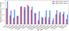Fig. 2

Relative abundances of the main isotopologues with respect to CH₃OH, towards IRAS 16293 A in red and IRAS 16293 B in blue. The abundances towards IRAS 16293 B are based on Persson et al. (2018) for H₂ CO, Lykke et al. (2017) for CH₃CHO, c-H₂ COCH₂, and CH₃ COCH₃, Jørgensen et al. (2016) for CH₂(OH)CHO and CH₃ COOH, and Jørgensen et al. (2018) for CH₂CO, CH₃ OCH₃, C₂ H₅OH, CH₃ OCHO, (CH₂ OH)₂, and t-HCOOH. We note that 30 and 10% of the uncertainties on the column density are considered for IRAS 16293 A and IRAS 16293 B, respectively.

Table 2

Rotational temperature, column density, and relative abundance with respect to CH₃ OH for the newlydetected species.

4 Discussion

4.1 Comparison between IRAS 16293 A and B

Most of the species and their isotopologues reported in this study are present towards both IRAS 16293 A and B; however, their abundances are different in a few cases.

Figure 2 shows the abundances of the main isotopologues with respect to CH₃OH towards IRAS 16293 A and B. The column densities, from which the abundances were der- ived, were determined by using the spectrum extracted from the offset positions, as described in the previous section for IRAS 16293 A, which were used in previous studies of IRAS 16293 B (Coutens et al. 2016; Lykke et al. 2017; Jørgensen et al. 2016). Towards IRAS 16293 A, the abundances relative to CH₃OH of CH₃OCHO, ethylene oxide (c-C₂H₄O), CH₃OCH₃, CH₃COCH₃, acetic acid (CH₃COOH), and HNCO are similar to the abundance observed towards IRAS 16293 B. On the other hand, the abundances of CH₂CO, H₂ CO, CH₃CHO C₂ H₅OH, CH₂(OH)CHO, (CH₂OH)₂, t-HCOOH, and forma- mide (NH₂CHO) are significantly lower towards IRAS 16293 A than those towards IRAS 16293 B. This selective differentiation could reflect the differentiation of the species across the two protostars. However, it is not possible to rule out the effects of the CH₃OH abundance with respectto H₂, for which the column density cannot be properly estimated. In addition, considering a single species as a reference for the abundance of all the species can interfere with the relation between the abundance of several species. For example, in the case of IRAS 16293 and the comet 67P/Churyumov-Gerasimenko, Drozdovskaya et al. (2019) show that itis more consistent to discuss the abundance of N-bearing and S-bearing species with respect to CH₃CN and CH₃SH, respectively.

In order to complete the picture, we estimated the statistical distance S of abundance ratios of each pair of species between IRAS 16293 A and B, as detailed in Appendix A. Figure 3 shows the colour map of this cross-comparison; each cell corresponds to the statistical distance of the abundance ratio of two species towards IRAS 16293 A as compared to IRAS 16293 B. The advantage of this comparative analysis is that the abundances do not rely on a single species. This technique offers a global view of the comparison in terms of molecular abundance between the offset position from the two sources. The first and the tenth rows of the map are shown in the right panels of the figure and correspond to the comparison of abundances relative to CH₃OH and C₂ H₅OH, respectively, towards IRAS 16293 A in comparison to IRAS 16293 B. The upper right panel shows a clear distinction between the similar abundance of species with respect to CH₃OH towards IRAS 16293 A and B as well as those with a higher abundance towards IRAS 16293 B in comparison to those towards IRAS 16293 A. This separation is represented with a vertical dashed line, between CH₃OCH₃ and HNCO. A similar separation, which is located between CH₂CO and H₂ CO, is shown on the lower right panel where the abundances are plotted with respect to C₂ H₅OH towards IRAS 16293 A in comparison to the abundances towards IRAS 16293 B. These separations represent a factor of two difference in the relative abundance ratio between IRAS 16293 A and B. This corresponds to a significance of 2σ, given the column density uncertainties.

The cross-comparison of all the main isotopologues between IRAS 16293 A and B suggests three distinct categories of species. The first category (noted Category I in Fig. 3) includes the species, such as CH₃OH, CH₃OCHO, c-C₂H₄O, CH₃COCH₃, CH₃COOH, CH₃OCH₂OH, t-C₂ H₅OCH₃, and CH₃OCH₃, which have similar abundances between IRAS 16293 A and B, or a low absolute statistical distance. H₂ CO, CH₃CHO, CH₂(OH)CHO, and (CH₂OH)₂ show a much lower abundance with respect to all the other species. This corresponds to the righter most part of the distance map (Category III in Fig. 3). The remaining species are in an intermediate category (Category II in Fig. 3) and are characterised by a lower abundance with respect to the first category species and a higher abundance with respect to the most depleted species for IRAS 16293 A in comparison to IRAS 16293 B. This comparative analysis suggests that there are at least two processes that deplete some of the species towards the offset position of IRAS 16293 A compared to the offset position of IRAS 16293 B. The possible causes of these depletions are discussed in the following sections.

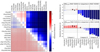Fig. 3

Left: cross-comparison of species from IRAS 16293 A in comparison to those from IRAS 16293 B. The statistical distance S is represented in the colour scale for each pair of species. One cell with a given value S of the plot should be read as “The abundance of the species X with respect to Y towards IRAS 16293 A is S sigma higheror lower compared to IRAS 16293 B”, with X and Y species taken from the X-axis and Y -axis, respectively. A positive value of S corresponds to N_X∕N_Y higher in IRAS 16293 A in comparison to IRAS 16293 B. Right: “CH₃OH” and “C₂ H₅OH” rows of the cross-comparison map. The two plots show the comparison of abundances with respect to CH₃ OH (upper panel) and C₂H₅OH (lower panel) towards IRAS 16293 A and IRAS 16293 B in terms of statistical distance.

4.2 Spatial extent

The spatial distribution of the emission towards IRAS 16293 A and B can be very different depending on the species. The deconvolved source size of the IRAS 16293 B continuum emission is estimated to be 0.′′ 5 (Jørgensen et al. 2016), which is similar to the beam size of the observations. Most of the detected species roughly follow the same distribution as the continuum and have the same source size. Concerning IRAS 16293 A, the continuum emission, as well as the molecular line emission arising from the gas, is more extended in the NE–SW axis where a 6 km s⁻¹ velocity gradient was reported (Pineda et al. 2012; Favre et al. 2014; Jørgensen et al. 2016; Oya et al. 2016). Small variations in the spatial distribution of different species towards IRAS 16293 A can be marginally resolved with the beam of PILS observations. However, the velocity gradient, which is associated with the very high line density that is present in the spectrum, makes it very difficult to integrate a single line across the source without contamination from nearby lines of other species.

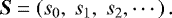
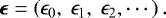
Calcutt et al. (2018b) developed a new method to map the emission, called the velocity integrated emission map (VINE map), which takes into account the velocity shift of the emitting gas when integrating over the molecular emission. At each pixel, the integration range is then shifted to the peak velocity of the line to be mapped. When there is no large velocity variation across the map, which is the case for IRAS 16293 B for instance, the VINE map is equivalent to the standard integrated emission map (moment zero map). For IRAS 16293 A, the velocity shift correction at each pixel of the VINE maps is based on the same bright transition 7_3,5−6_4,4 of CH₃OH at 337.519 GHz as used by Calcutt et al. (2018b). This transition is particularly suited for tracing the hot corino while being well isolated from other lines. Figure 4 shows VINE maps of the main isotopologues, and few deuterated conformers were detected towards IRAS 16293 A. In this study, the VINE maps were only used to check whether the emission distribution reaches the offset position, where we analysed the spectrum, as indicated by the white cross.

The emission of the species that have similar abundances towards IRAS 16293 A and B is distributed along the velocity gradient direction and cover the offset position, whereas the emission distribution of the depleted species towards IRAS 16293 A in comparison to IRAS 16293 B is located around the continuum peak position of the respective sources and does not show the elliptical distribution of the continuum emission towards IRAS 16293 A. Only the CH₃COOH emission distribution is as compact as the (CH₂OH)₂ emission distribution, while the abundance towards IRAS 16293 A and B are similar. We checked the distribution emission towards IRAS 16293 B as well as for this species and noticed that the emission does not cover the offset position used in the previous studies. Therefore, CH₃COOH seems depleted towards both IRAS 16293 A and B. This is why CH₃COOH does not show a difference between IRAS 16293 A and B since it belongs to the most compact region of the warm envelope.

Spatial differences between COMs were previously observed towards the Galactic Centre Sgr B2 region (Hollis et al. 2001) as well as towards high-mass protostars (for example, Calcutt et al. 2014). Hollis et al. (2001) observed the emission of CH₃OCHO and CH₂(OH)CHO, among others, at two different angular resolutions. They detected the two species with an ~60″ beam size using the NRAO 12 m telescope, whereas the Berkeley-Illinois-Maryland Association (BIMA) observations with a beam of ~5″ only revealed CH₃OCHO. They suggested that CH₂(OH)CHO was much more extended compared to CH₃OCHO and its emission was spatially filtered by the interferometric character of the observations. These findings are supported by the more recent study of Li et al. (2017) towards an extended region of the Galactic Centre in which the authors reported cold gas emission of CH₂(OH)CHO ~36 pc in width around Sgr B2(N). We note that, these two observations of the CH₂(OH)CHO spatial extent are specific to the Galactic Centre, where non-thermal desorption processes put the CH₂(OH)CHO in the gas phase at temperatures much lower than the thermal desorption temperature of this species.

Xue et al. (2019) consistently observed the three isomers CH₃COOH, CH₃OCHO, and CH₂(OH)CHO towards Sgr B2(N) using ALMA in Band 3 with an angular resolution of 1.′′ 6, which is sufficient to resolve the sources. The spatial distribution of the species reveals that CH₃OCHO is more extended than both CH₂(OH)CHO and CH₃COOH, which is in agreement with the present study. Xue et al. (2019) suggest that the different formation pathways of the tree species through ice surfaces and gas-phase chemistry could explain the spatial differentiation. This interpretation was supported by the correlation with the distribution of the respective precursors especially for gas-phase formation, such as CH₃OCH₃, which is the precursor of CH₃OCHO (Balucani et al. 2015), and C₂ H₅OH the precursor of CH₂(OH)CHO and CH₃COOH (Skouteris et al. 2018). The search for precursors through ice surfaces formation pathway is limited by the current infra-red absorption observations. Alternatively, the authors suggest that the effective desorption temperature of the species could explain their spatial distribution difference based on temperature-programmed desorption (TPD) experiments of C₂ H₄O₂ isomers (Burke et al. 2015). During the TPD, CH₃OCHO desorbed at ~70 K whereas CH₂(OH)CHO and CH₃COOH were released in the gas phase at ~110 K. In the warm-up model of star formation, this would result in a more extended emission of CH₃OCHO in comparison to the two other isomers.

Calcutt et al. (2014) simultaneously detected CH₃OCHO and CH₂(OH)CHO, among other species, towards three high-mass sources, G31.41+0.31, G29.96–0.02, and G24.78+0.08A, which are located at 3.5, 7.1, and 7.7 kpc away, respectively. They find that CH₃OCHO was more extended than CH₂(OH)CHO towards G31 and that the two species had the same extent towards the two other sources. The spatial differentiation found in G31 could be similar to IRAS 16293; however, CH₂(OH)CHO and the other depleted species towards IRAS 16293 A could also trace a deeper region in the envelope due to the excitation conditions. For example, CH₃OCHO lines are optically thicker than those of CH₂(OH)CHO and show a more extended spatial distribution.

Also, such a spatial differentiation can be inferred indirectly. The first detection of glycolaldehyde by Jørgensen et al. (2012) was performed with ALMA at ~2″ angular resolution: This is enough to separate the two components of the binary system but larger than the source size of both components. Jørgensen et al. (2012) find a relative abundance CH₃OCHO/CH₂(OH)CHO of 10–15 for both protostars on these scales and did not see the same evidence for depletion of CH₂(OH)CHO with respect to CH₃OCHO for IRAS 16293 A in comparison to IRAS 16293 B, as discussed above. However, it is consistent with the interpretation that CH₂(OH)CHO, as well as the other most depleted species towards the offset position from IRAS 16293 A, are located in a more compact region of the hot corino. This is also supported by observations of other COMs, such as CH₃OCH₃, D₂ CO (Jørgensen et al. 2011) and C₂ H₅OH (Bisschop et al. 2008).

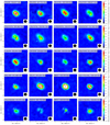Fig. 4

Representative velocity integrated emission maps of the detected COMs towards IRAS 16293 A. The black and white crosses indicate the continuum peak position and the offset position, respectively. The species and the line frequency are noted in the top-left corner and the 0.′′ 5 beam is shown in the bottom right corner of each panels.

4.3 Differentiation in rotational temperature

The distribution of COMs towards IRAS 16293 A suggests that a significant part of the emission is missing at the extracted spectrum position. However, the estimation of the rotational temperature is sensitive to the intensity variation of one line with respect to another line with a different upper energy level. Thus, the derivation of the rotational temperatureis not affected by the apparent depletion due to the spatial extent and can be securely compared species-to-species.

Towards IRAS 16293 A, the rotational temperatures of the detected species and their isotopologues are between 90 and 180 K, where HNCO, H₂CO, CH₂(OH)CHO, (CH₂OH)₂, NH₂CHO, CH₃CHO, and C₂ H₅OH are the hottest species. Although the distinction between those hot species and the other species is not pronounced, the hot species seem to be located closer to the protostars compared to the other species, showing a lower rotational temperature.

Using the PILS observations towards IRAS 16293 B, Jørgensen et al. (2018) detected the same species as those presen- ted in this study and derived their rotational temperature. The authors find that the species located in the hot corino couldbe distinguished into two groups depending on their rotational temperature. Species such as CH₃OH, C₂ H₅OH, CH₃OCHO, NH₂CHO, HNCO, CH₂(OH)CHO, and (CH₂OH)₂ were observed with an rotational temperature of 250–300 K, whereas CH₂CO, CH₃CHO, CH₃OCH₃, H₂ CO, and c-H₂COCH₂ were found at 100–150 K. Using these results and the previous results of PILS observations towards IRAS 16293 B from Coutens et al. (2016), Jørgensen et al. (2016), and Persson et al. (2018), Jørgensen et al. (2018) find a correlation between the rotational temperature and the desorption temperature of the oxygen-bearing COMs that are thought to mainly form on ice surfaces. This implies that the species that have a high rotational temperature (250–300 K) are more predominantly located in the hot and compact region of the hot corino, while the lower rotational temperature species belong to a more extended region inside the hot corino (see Fig. 4 of Jørgensen et al. 2018). By comparing this scenario to the difference in the spatial extent observed in IRAS 16293 A, the compact species, such as CH₂(OH)CHO, (CH₂OH)₂, NH₂CHO, HNCO, and C₂ H₅OH, are associated with high rotational temperature, whereas extended species, such as c-H₂COCH₂, CH₃OCH₃, and CH₃COCH₃, have a low rotational temperature. The ordering of the species across the onion-like structure of the envelope is in agreement with the desorption temperatures observed in temperature-programmed desorption (TPD) experiments of pure and mixed ices (Öberg et al. 2009; Fedoseev et al. 2015a,b, 2017; Paardekooper et al. 2016; Chuang et al. 2016; Qasim et al. 2019a,b).

In addition, the rotational temperature of CH₃COOH towards IRAS 16293 B is consistent with its most compact location in the envelope of both sources. However, the correlation between the rotational temperature and the location does not work in IRAS 16293 A for CH₃OH, CH₃OCHO, CH₂CO, H₂ CO, CH₃CHO, and t-HCOOH.

Concerning CH₃OH and CH₃OCHO, these two species were found to be hot species in IRAS 16293 B; however, they correspond to cold and extended species in IRAS 16293 A. Their optically thick lines suggest the presence of two components towards IRAS 16293 B that are indistinguishable due to the smaller source size with respect to the angular resolution: one is at a rotational temperature of 300 and another is at ~125 K (Jørgensen et al. 2018). In addition, the rotational temperature derived towards IRAS 16293 A for the same two species is only consistent with the second component at 125 K, indicating that the bulk of the emission consists of the extended warm gas. From this, CH₃OH and CH₃OCHO are found totrace not only the central core but also the extended part of the hot corino.

Regarding CH₂CO isotopologues, there are only a few lines in the range of the observations and most of those are blended with small species, such as ³³ SO at ~343.08 GHz and CS at ~342.88 GHz. The deuterated isotopologue CHDCO suggests that the low abundance towards IRAS 16293 A compared to IRAS 16293 B is due to the spatial extent differences between the two sources. The emission distribution of H₂ CO was found to be much more complex and extended across the binary protostars and it traces both the hot corino region and the outflow interface with the bridge structure between IRAS 16293 A and B and the E–W outflow emerging from IRAS 16293 A (van der Wiel et al. 2019).

The few unblended, but optically thick, lines of CH₃CHO show a large distribution towards both sources, suggesting that the bulk of the emission corresponds to the extended part of the hot corino, despite the abundance difference between sources A and B. The three-phase chemical model of Garrod (2013) shows that the abundance of CH₃CHO in the gas phase increases during the evolution of the hot corino, which occurs even before the species desorbs from the ice grain surfaces. This suggests that gas-phase formation paths significantly contribute to the formation of CH₃CHO at relatively low temperatures before the bulk of the species desorb from the ice. Concerning the abundance observed towards IRAS 16293 binary, if the gas-phase formation paths effectively produce CH₃CHO in the outer part of the hot corino, it should increase the abundance of CH₃CHO towards the most luminous source with respect to the other component. However, the luminosity of IRAS 16293 A was estimated to be ~ 18 L_⊙, which is six times higher than IRAS 16293 B (Jacobsen et al. 2018).

In summary, the analysis of the spatial extent, the abundances, and the rotational temperatures suggests that the hot corinos show a stratification of the COMs along the distance to the forming star. This spatial differentiation towards IRAS 16293 A could be linked to the rotational temperature of the species observed towards IRAS 16293 B in the way that species at 300 K are more compact than the species at 125 K. Although this spatial differentiation is not resolved for IRAS 16293 B, the rotational temperature suggests its presence. Towards IRAS 16293 A, the difference in rotational temperaturebetween compact and extended species is less pronounced, which could be due to the geometry of the source (inclination, size) or the presence of the nearly edge-on disc (Pineda et al. 2012; Favre et al. 2014; Girart et al. 2014).

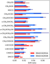Fig. 5

D/H ratio of the deuterated species detected towards IRAS 16293 A in red and IRAS 16293 B in blue. The D/H ratio is calculated from the abundance ratio, with the statistical correction due to the chemical group (see Appendix B of Manigand et al. 2019). D/H ratios towards IRAS 16293 B are taken from Coutens et al. (2016), Lykke et al. (2017), Persson et al. (2018), and Jørgensen et al. (2018).

4.4 D/H ratio

The sensitivity of the ALMA observations makes the detection of many deuterated isotopologues of the oxygen-bearing species possible. Figure 5 compares the D/H ratios of these species derived from the estimated column densities found towards the offset position of IRAS 16293 A and reported in the previous studies of IRAS 16293 B (Coutens et al. 2016; Lykke et al. 2017; Persson et al. 2018; Jørgensen et al. 2018) on a linear scale. In general, the D/H ratios of IRAS 16293 A species are found to be as high as those of the species of IRAS 16293 B. However, due to the higher uncertainty in the column densities and the higher number of upper limits, it is difficult to observe a trend in the deuteration itself. Nevertheless, there is apparently no direct correlation between the D/H ratios and the stratification suggested by the rotational temperatures. This could suggest that contrary to the rotational temperatures and the spatial extents, which give a clue as to the structure of the hot corino and thus the warm chemistry in situ, the D/H ratio gives information about the history of the envelope during the pre-stellar phase when the gas was cold enough to let the D/H ratio of the frozen species increase. This is supported by the D/H ratio of the doubly-deuterated isotopologues D₂ CO of 2.0 ± 0.4 × 10⁻¹ and CHD₂OCHO of 8.2 ± 0.6 × 10⁻² (Manigand et al. 2019) found towards IRAS 16293 A.

Using the result reported in Table 2 and the column density of CH₃CHO measured towards IRAS 16293 B (Lykke et al. 2017; Jørgensen et al. 2018), which is 1.2 × 10¹⁷ cm⁻², the D/H ratio of CH₂DCHO and CH₃CDO are 1.4 and 4.7%, respectively. The upper limits of the D/H ratio of CH₂DCHO and CH₃CDO towards IRAS 16293 A are <6 and < 17%, respectively. The D/H ratio of the groups CH₃– and HCO– are significantly different for CH₃CHO even after applying the statistical correction for both sources. Assuming that the main formation route is due to the addition of those two radicals on the ice surface during the warm-up phase, then the difference in deuteration may indicate that the deuteration enhancement is different for CH₃ and HCO, which are already in the prestellar phase when the temperature is low enough to favour the deuteration enhancement of H $_{3}^{+}$ $_3^+$ in the gas phase. However, the other species thought to be formed on ice surfaces do not show such a difference in the D/H ratio between CH₃– or CH₂– and HCO– groups, such as CH₃OCHO and CH₂(OH)CHO (Jørgensen et al. 2016). This suggests a selective process, independent of the luminosity difference between IRAS 16293 A and B, which increases the deuteration of HCO– or decreases those of CH₃– without significantly impacting the other species.

As a side note, the high intensity of the candidate lines found for CHD₂OH in the range of the observations and the enhancement of the D/H ratio of the two doubly-deuterated isotopologues D₂ CO and CHD₂OCHO with respect to their respective singly-deuterated isotopologues, HDCO and CH₂DOCHO, suggest a roughly equally high column density for CHD₂OH. This stresses the importance of future studies on the spectroscopy of CHD₂OH and even more its deuterated conformers CD₃OH and CD₃OD.

5 Conclusions

In this study, we analysed the molecular content of the protostar IRAS 16293 A at the hot corino scale and compared the abundances to those measured towards its protostar companion IRAS 16293 B. Numerous O-bearing species have been detected, along with their rarer isotopologues. The main findings of this work are summarised below.

1.
The abundances with respect to CH₃OH of half of the species are significantly lower towards the 0.′′ 6 offset position from IRAS 16293 A in comparison to the 0.′′ 5 offset position from IRAS 16293 B in spite of its higher luminosity.
2.
The cross-correlation of the main isotopologue abundances highlights a selective differentiation depending on the species observed. Different categories are identified whether the species abundances are similar or significantly different between IRAS 16293 A and B.
3.
The first category, including CH₃OH, CH₃OCHO, c-C₂H₄O, CH₃COCH₃, CH₃COOH, CH₃OCH₃, t-C₂H₅OCH₃, and CH₃OCH₂OH, corresponds to the species that have a similar abundance towards both IRAS 16293 A and B. These species show an extended spatial distribution across IRAS 16293 A and have a relatively low rotational temperature of ~125 K towards IRAS 16293 B, except for CH₃COOH, CH₃OH and CH₃OCHO. CH₃COOH spatial distribution is much more compact towards both IRAS 16293 A and B than the other extended species and the rotational temperature found towards IRAS 16293 B, which is unambiguously ~300 K. In addition, CH₃OH and CH₃OCHO show attributes of both compact and extended regions as suggested by their extended distribution and their high desorption temperature. Their emission is suspected to trace both regions in the hot corino.
4.
The second category concerns the species showing a significantly lower abundance towards IRAS 16293 A with respect to IRAS 16293 B, which are HNCO, C₂H₅CHO, C₂H₅OH, t-HCOOH, NH₂CHO, CH₂CO, H₂CO, CH₃CHO, CH₂(OH)CHO, and (CH₂OH)₂. These species have a more compact spatial distribution towards IRAS 16293 A compared to the first category of species. In addition, they tend to have a high rotational temperature of ~300 K, especially for those that are the most compact, such as CH₂(OH)CHO and (CH₂OH)₂. However, the spatial distribution difference is not resolved towards IRAS 16293 B, the rotational temperature difference between compact and extended species is more pronounced though. H₂CO, CH₂CO, and CH₃CHO do not fit into any category as they have a roughly compact spatial emission but a low rotational temperature.
5.
In the search for O-bearing species, we report the new detection of t-C₂H₅OCH₃ and CH₃OCH₂OH towards IRAS 16293 B. Their abundances with respect to CH₃OH are consistent with the previous detection of these species towards the high mass protostellar regions Sgr B2(N) and Orion KL. Upper limits of their column density are derived towards IRAS 16293 A.
6.
The D/H ratio is not correlated to the structure of the hot corino itself; however, it is the result of what happens during the formation of COMs in the pre-stellar phase. The multiply-deuterated COMs seem to have a systematically higher D/H ratio compared to singly-deuterated species. More observations of different sources, supported by future spectroscopic studies of other multiply-deuterated COMs, are required to confirm this trend. In addition, we report the identification of 23 CHD₂OH transitions at 0.8 mm wavelength, which have not been observed so far. The intensity of CHD₂OH lines suggests a high abundance and D/H ratio, as it is for CHD₂OCHO. The identification of these CHD₂OH transitions highlights the need for spectroscopic data for CHD₂OH and CD₃OH to derive their rotational temperatures and their column densities and to get their D/H ratios.

As discussed in this paper, abundance variations between IRAS 16293 A and B suggest that the spatial distributions are different for the species associated with low or high rotational temperatures. Whether the origins of these differences are physical or chemical,future higher angular observations will be critical in resolving the innermost structure of the two protostars.

Acknowledgements

The authors wish to thank the anonymous referee for the constructive comments that significantly improved the paper. The authors are grateful to Brett McGuire and Roman Motiyenko for providing the line strengths of CH₃OCH₂OH spectroscopic data. The authors acknowledge Gleb Fedoseev for the valuable discussion about the desorption temperatures from the TPD experiments of the O-bearing COMs and Troels C. Petersen for discussions of the statistical methods. This paper makes use of the following ALMA data: ADS/JAO.ALMA#2012.1.00712.S and ADS/JAO.ALMA#2013.1.00278.S. ALMA is a partnership of ESO (representing its member states), NSF (USA) and NINS (Japan), together with NRC (Canada), NSC and ASIAA (Taiwan), and KASI (Republic of Korea), in cooperation with the Republic of Chile. The Joint ALMA Observatory is operated by ESO, AUI/NRAO and NAOJ. The group of J.K.J. acknowledges support from the H2020 European Research Council (ERC) (grant agreement No 646908) through ERC Consolidator Grant “S4F”. Research at Centre for Star and Planet Formation is funded by the Danish National Research Foundation. A.C. postdoctoral grant is funded by the ERC Starting Grant 3DICE (grant agreement 336474). M.N.D. is supported by the Swiss National Science Foundation (SNSF) Ambizione grant 180079, the Center for Space and Habitability (CSH) Fellowship and the IAU Gruber Foundation Fellowship. This research has made use of NASA’s Astrophysics Data System and VizierR catalogue access tool, CDS, Strasbourg, France (Ochsenbein et al. 2000), as well as community-developed core Python packages for astronomy and scientific computing including Astropy (Astropy Collaboration 2013), Scipy (Jones et al. 2001), Numpy (van der Walt et al. 2011) and Matplotlib (Hunter 2007).

Appendix A: Statistical distance

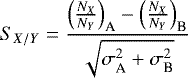
The statistical distance of the abundance of a species X relative to a species Y between IRAS 16293 A and IRAS 16293 B is calculated as follows: $S_{X / Y} = \frac{{(\frac{N_{X}}{N_{Y}})}_{A} - {(\frac{N_{X}}{N_{Y}})}_{B}}{\sqrt{σ_{A}^{2} + σ_{B}^{2}}}$ $\begin{equation*} S_{X/Y} = \frac{\left(\frac{N_X}{N_Y}\right)_{\text{A}} - \left(\frac{N_X}{N_Y}\right)_{\text{B}}}{ \sqrt{\sigma_{\text{A}}^2 + \sigma_{\text{B}}^2}} \end{equation*}$ (A.1)

in which σ_A and σ_B are the uncertainties of the column density ratios ${(\frac{N_{X}}{N_{Y}})}_{A}$ $\left(\frac{N_X}{N_Y}\right)_{\text{A}}$ and ${(\frac{N_{X}}{N_{Y}})}_{B}$ $\left(\frac{N_X}{N_Y}\right)_{\text{B}}$ , respectively. The value ofS_X∕Y correspondsto the significance of the distance in terms of the number of σ.

Appendix B: Monte-Carlo error estimation

Because of the non-linearity of the model used in this study and the non-standard χ² minimisation method, the uncertainties on the excitation temperature and the column density are not derivable from the covariance matrix, usually calculated with the χ² minimisation methods. In this case, the Monte Carlo (MC) simulation becomes a convenient tool to estimate the uncertainties from the posterior probability distributions of each parameter of the model. In this section, we describe the bootstrap algorithm, which is a specific class of Monte Carlo simulations, that was tested to estimate the uncertainties of the parameters of the model.

Consider the data fitted as a vector S of N elements, which are the data points: $S = (s_{0}, s_{1}, s_{2}, \dots) .$ $\begin{equation*} \vec{S} = \left(s_0,~s_1,~s_2, \cdots\right) .\end{equation*}$ (B.1)

A Gaussian noise ɛ is defined with the same logic: $ɛ = (ɛ_{0}, ɛ_{1}, ɛ_{2}, \dots) .$ $\begin{equation*} \vec{\epsilon} =\left(\epsilon_0,~\epsilon_1,~\epsilon_2,\cdots\right) .\end{equation*}$ (B.2)

The χ² minimisation can be represented by a function $F_{χ^{2}}$ $F_{\chi^2}$ that transforms a data vector S into a parameter vector P, which is the best fit parameters of the model for the given data. The inverse function F⁻¹ is thus the fitting model, that is, the synthetic spectrum in the present study: $\begin{array}{l} P = (p_{0}, p_{1}, p_{2}, \dots) \\ F_{χ^{2}} : S \to F_{χ^{2}} (S) = P \\ F^{- 1} : P \to F^{- 1} (P) = \tilde{S} \end{array}$ $\begin{align*} &\vec{P}=\left(p_0,~p_1,~p_2, \cdots\right) \\ &F_{\chi^2}:\vec{S} \longrightarrow F_{\chi^2}(\vec{S}) = \vec{P} \\ &F^{-1}:\vec{P} \longrightarrow F^{-1}(\vec{P}) = \vec{\tilde{S}} \end{align*}$

in which $\tilde{S}$ $\vec{\tilde{S}}$ is the closest synthetic spectrum to the data S. The MC method used in this study is a simple application of the Markov-chain MC simulations where: the prior distribution is a group of normally distributed noise ${ɛ_{i}}_{N_{MC}}$ $\left\{\vec{\epsilon}_i\right\}_{N_{\textrm{MC}}}$ of a width equivalent to the uncertainty σ of the data, with N_MC the total number of walkers; the sampler is the χ² minimisation function $F_{χ^{2}}$ $F_{\chi^2}$ ; the probability for a walker to jump to a worse position in the parameter space is null; and only the final position of each walker is kept.

In this particular case, the posterior probability distributions are fully dependent on the prior distributions. From the MC simulation, we get a group of parameter vectors: $\begin{array}{l} P = {F_{χ 2} (S + ɛ_{i})}_{N_{MC}} \\ = {{(p_{0}, p_{1}, p_{2}, \dots)}_{0}, {(p_{0}, p_{1}, p_{2}, \dots)}_{1}, \dots}_{N_{MC}} \\ P^{T} = ({p_{0}}_{N_{MC}}, {p_{1}}_{N_{MC}}, {p_{2}}_{N_{MC}}, \dots) \\ P^{T} = (P_{0}, P_{1}, P_{2}, \dots), \end{array}$ $\begin{align*} &\mathcal{P} = \left\{ F_{\chi2}\left(\vec{S} + \vec{\epsilon_i} \right)\right\}_{N_{\textrm{MC}}} \\ &\ \ \ = \left\{ (p_0,~p_1,~p_2,\cdots)_0,~(p_0,~p_1,~p_2,\cdots)_1,\cdots\right\}_{N_{\textrm{MC}}} \\ &\mathcal{P}^T= \left(\left\{p_0\right\}_{N_{\textrm{MC}}},~\left\{p_1\right\}_{N_{\textrm{MC}}},~\left\{p_2\right\}_{N_{\textrm{MC}}},\cdots\right) \\ &\mathcal{P}^T= \left(\mathcal{P}_0,~\mathcal{P}_1,~\mathcal{P}_2,\cdots\right), \end{align*}$

where $P_{i}$ $\mathcal{P}_i$ is the group of parameters p_i. The distribution of $P_{i}$ $\mathcal{P}_i$ , called the posterior probability distribution of p_i, gives the needed information for the fitted parameters. It is maximal for the best fit value and the width at half-maximum of each side of the distribution corresponds to the negative and positive uncertainties on p_i.

Appendix C: Laboratory spectroscopic data

Most of the analysed species do not assume any excited vibrational or torsional level contributions to the partition function at low rotational temperatures. However, they are all detected at rotational temperatures above 100 K, where the vibrational and torsional contribution can be significant. Thus, it is necessary to detail the spectroscopic dataset used for each species. In this study, a vibrational correction factor > 1.1 is considered significant and is not applied to the column density derived from the synthetic spectrum fit if it lies below this value.

Spectroscopic data for CH $_{3}^{18}$ $_3^{18}$ OH are provided in the Cologne Database of Molecular Spectroscopy² (CDMS, Endres et al. 2016 and Müller et al. 2005, 2001) from the spectroscopic analyses of Fisher et al. (2007) and Ikeda et al. (1998). The entry of ¹³ CH₃OH, from the CDMS catalogue, is based on Xu & Lovas (1997) and Xu et al. (1996). The dipole moment is assumed to be the same as of the main isotopomer, and the partition function takes only the permanent dipole moment into account. The spectroscopy of CH₂DOH is taken from the Jet Propulsion Laboratory catalogue³ (JPL, Pickett et al. 1998), where the entry is based on Pearson et al. (2012). The frequency list for CHD₂OH is based on Ndao et al. (2016), with additional transitions in the range of the PILS observations from Mukhopadhyay (2016). The data do not include line strengths or the partition function; however, the frequencies are assigned with uncertainty much lower than the resolution of the observations used in this study.

The spectroscopic data for CH₃OCHO isotopologues, except for CH₃O¹³CHO, are described in Manigand et al. (2019), and references therein, from which the derived column densities for source A are taken. The CDMS entry for CH₃O¹³CHO is based on Carvajal et al. (2010), with measured data in the range of the PILS survey from Willaert et al. (2006) and Maeda et al. (2008a,b). The vibrational contribution of CH₃O¹³CHO is already included in the CDMS entry (Favre et al. 2014).

The data for CH₃OCH₃ are provided by the CDMS catalogue. The entry is based on Endres et al. (2009) with additional data in the range of our survey from Groner et al. (1998). The mono-deuterated dimethyl ether (CH₂DOCH₃) exists in two forms, symmetric and asymmetric. The data of both conformers are taken from Richard et al. (2013). The data of CH₃O¹³CH₃ are taken from Koerber et al. (2013) and from the Vizier Online Data Catalogue, which is from the Centre de Données Astronomiques de Strasbourg⁴ (CDS). The contribution from excited vibrational levels is estimated to be 1.15 at T_ex = 100 K for the ¹³C and deuterated isotopologues.

Spectroscopic data for CH₃CHO can be found in the JPL catalogue. The entry is based on Kleiner et al. (1996), with experimental transition frequencies in the range of our survey from Belov et al. (1993). The CDMS entry for CH₃CDO is based on Coudert et al. (2019). The fit and the experimental frequencies used are described in Elkeurti et al. (2010), with additional data below 50 GHz taken from Martinache & Bauder (1989). The partition function includes the first three excited torsional mode contributions and is reliable at 140 K. The spectroscopy of the other deuterated isotopologue CH₂DCHO is also described in Coudert et al. (2019) with additional data taken from Turner & Cox (1976) and Turner et al. (1981). The contribution of the lowest torsional mode and the small amplitude vibration are included in the partition function. The partition function converged up to about 100 K. Therefore, vibrational corrections are neglected at 140 K.

C₂ H₅OH isotopologues exist under two isomeric forms, anti and gauche, depending on the OH group torsion. In addition, the gauche conformer has two degenerated states. The extended analysis of the vibrational ground state is provided by Pearson et al. (2008). However, Müller et al. (2016) find that the predicted intensities do not fit the Sgr B2(N2) emission at 3 mm, and they provide a corrected entry in the CDMS catalogue. This entry combines the anti and the gauche conformer transitions and includes data from Pearson et al. (1995, 1996) in the range of the PILS survey. ¹³ C and deuterated C₂ H₅OH isotopologues spectroscopic data are taken from corresponding CDMS entries, based on Bouchez et al. (2012) and Walters et al. (2015), respectively. However, these data consider only the anti conformer. The column density has to be multiplied by a factor of ~2.32 at T_ex = 135 K to take the gauche conformer into account (Müller et al. 2016; Jørgensen et al. 2018). The contribution from excited vibrational levels is dominated by the two torsional modes of the methyl group (Durig & Larsen 1990)⁵. The vibrational correction factor is 1.24 for the main isotopologue (Durig et al. 2011) and is applicable for the ¹³ C and deuterated isotopologues.

Spectroscopic data of the H₂CO isotopologues are taken from the corresponding CDMS entries and are the result of several contributions over the past four decades. H₂ CO, H₂ C¹⁸O and H₂ C¹⁷O entries are based on Müller & Lewen (2017), the H $_{2}^{13}$ $_2^{13}$ CO entry is based on Müller et al. (2000a), and HDCO and D₂ CO entries are based on Zakharenko et al. (2015). Additional data were taken from Brünken et al. (2003), Bocquet et al. (1996), and Cornet & Winnewisser (1980) for H₂ CO as well as a few transition frequencies of H₂ C¹⁸O and H $_{2}^{13}$ $_2^{13}$ CO. Müller et al. (2000c) provided the ground state combination differences employed in the spectroscopic analysis of H₂ CO. For the two deuterated isotopologues HDCO and D₂CO, the data were taken from Lohilahti & Horneman (2004), Bocquet et al. (1999), and Dangoisse et al. (1978). Additional H₂ C¹⁸O transition frequencies were taken from Müller et al. (2000b). The dipole moments were measured by Fabricant et al. (1977) and Johns & McKellar (1977). The dipole moments of H₂ C¹⁷O and H₂ C¹⁸O are assumed to be the same as the H₂CO one. The vibration state energies are way too high to significantly affect the partition function at 155 K.

The publicly available JPL entry for CH₃COCH₃, also called propanone, is based on Groner et al. (2002), with the rotational partitioning and the line strength calculation. This study used additional data from Oldag & Sutter (1992), Vacherand et al. (1986), and Peter & Dreizler (1965) for transition frequencies up to 300 GHz. In the present study, we used an updated version of the spectroscopic data, which will be available on CDMS. This entry is based on the study of Ordu et al. (2019), which includes the previous linelists as well as those from the first two torsional excited states taken from Morina et al. (2019) and Groner et al. (2006). The contribution from excited vibrational level ν = 1 is taken into account in the harmonic approximation and thus in the partition function.

c-H₂COCH₂ data are provided by the CDMS catalogue. The entry was based on experimental data taken from Hirose (1974), Creswell & Schwendeman (1974), and Pan et al. (1998). Much more additional data from Medcraft et al. (2012) enriched the set, extending the frequency range from 358 GHz to 4 THz. The dipole moment is taken from Cunningham et al. (1951). The vibrational correction factor is insignificant at 95 K.

The rotational spectrum of CH₃COOH was first extensively analysed by Ilyushin et al. (2008), which was based on a fair amount of measured spectroscopic data from 8 to 358 GHz taken from Tabor (1957), Krisher & Saegebarth (1971), van Eijck et al. (1981), van Eijck & vanDuijneveldt (1983), Demaison et al. (1982), Wlodarczak & Demaison (1988), and Ilyushin et al. (2001, 2003). The present study uses the recent datafile provided by Ilyushin et al. (2013). This last study considerably extended the number of measured transition frequencies up to 845 GHz and observed the first two torsional excited states. The partition function takes into account these states and more excited torsional up to v_t = 8 in the vibrational ground state. The low vibration states are too energetically high to make the vibrational correction factor significant at 110 K.

The JPL catalogue provides the line list for CH₂(OH)CHO. The entry isbased on the rotational lines collection of Carroll et al. (2010). Previous laboratory measurements were carriedout by Marstokk & Møllendal (1970, 1973), and Butler et al. (2001) and served as the base for the latest study. The partition function was previously calculated by Widicus Weaver et al. (2005) over a measured frequency range from 72 to 122.5 GHz and included the ground state and three partially populated vibrational states at room temperature. Carroll et al. (2010) find a systematic bias in the lines with K_a ~ 28−31 and they corrected iteratively the assignment in the JPL line list.

NH₂CHO data used inthis study are provided by the CDMS catalogue. The dipole moment was measured by Kurland & Bright Wilson (1957). The observed experimental frequencies are taken from Kukolich & Nelson (1971), Nielsen (1973), Hirota et al. (1974), Gardner et al. (1980), Moskienko & Dyubko (1991), Vorob’eva & Dyubko (1994), Blanco et al. (2006), and Kryvda et al. (2009). The latest study (Motiyenko et al. 2012) considerably extended the frequency range of measured transitions up to 930 GHz. The partition function does not include any contributions from the excited vibrational state. However, the lowest vibration state energy of 288 cm⁻¹ leads to the highest vibration correction factor, which is lower than 1.1 at 145 K.

Spectroscopic data of the HCOOH isotopologues are provided in the CDMS catalogue for t-HCOOH and by JPL for t-H¹³COOH, t-DCOOH, and t-HCOOD. The CDMS entry for the main isotopologue is based on Winnewisser et al. (2002) with additional data from previous studies (Auwera 1992; Willemot et al. 1980). The JPL entries are based on the same study of Lattanzi et al. (2008) gathering the analysis of these three isotopologues. Experimental measurements were taken from Bellet et al. (1971) and Lerner et al. (1957) for the three entries, and Wellington Davis et al. (1980) and Winnewisser et al. (2002) only for the t-H¹³COOH entry. The dipole moment is assumed to be the same as the main isotopologue, which was measured by Kuze et al. (1982). The excited vibrational state, especially ν₇ and ν₉, was also measured for the ¹³C and deuterated isotopologues in the studies of Baskakov et al. (1999, 2006) and Baskakov (1996). Vibration correction factors are neglected at 90 K for both the main and deuterated species.

The CDMS entries for CH₂CO isotopologues are based on Guarnieri & Huckaufa (2003) and on Guarnieri (2005) for the deuterated isotopologues (CHDCO). Laboratory measurements of the different isotopologues are taken from Johnson & Strandberg (1952), Brown et al. (1990), Johns et al. (1992), and Sutter & Dreizler (2000). The dipole moments were calculated by Fabricant et al. (1977). Vibrations contributions are negligible at 135 K for both isotopologues.

(CH₂OH)₂ has three coupled rotors along the molecular chain. It can exist in a total of ten stable configurations (Christen et al. 2001) based on the orientation of the two OH groups at both ends of the carbon chain. Most of the transitions, especially the low-energy rotational transitions, are emitted from the two lowest fundamental state conformers aGg′-(CH₂OH)₂ and gGg′-(CH₂OH)₂, the second one lying 290 K above aGg′ (Müller & Christen 2004). The spectroscopic data used here are taken from the CDMS entries. Experimental measurements and extensive analysis were carried out by Christen et al. (1995) and Christen & Müller (2003) for aGg′ and by Christen et al. (2001), and Müller & Christen (2004) for gGg′, up to 370 and 579 GHz, respectively. Concerning the gGg′ conformer, the line strength and partition function were treated as if the conformer was the lowest conformer energy. The ground state energy of 290 K contributes to the line strengths by a factor of 2.35 at 145 K (Müller & Christen 2004). The vibrational correction factor at 145 K of 1.75, which includes the interactions between gGg′ and aGg′, were calculated in the anharmonic approximation from Boussessi et al. (2016) for both conformers.

t-C₂ H₅OCH₃ data were taken from a preliminary CDMS entry. They are based on Fuchs et al. (2003), with significant additional data from Kobayashi et al. (2016) as well as the experimental measurements from Hayashi & Adachi (1982) and Tsunekawa et al. (2003, 2011). The dipole moment was measured by Hayashi & Kuwada (1975). Torsional and vibrational transitions were studied by Senent et al. (2009), providing a future basis for determining the contribution of higher vibrational state energies to the partition function. The partition function and the line strength were revised by H. S. P. Müller. With the lowest vibrations at 288 cm⁻¹, the vibrational correction factor is negligible.

Regarding HNCO isotopologues, the spectroscopic data are taken from the CDMS entry for HNCO, and from the JPL entry for DNCO. The CDMS entry is based on the work of Lapinov et al. (2007), using additional data from Kukolich & Nelson (1971), Hocking et al. (1975), and Niedenhoff et al. (1995). The JPL entry was last updated in 1987 and only includes the frequencies from Hocking et al. (1975). However, the frequency uncertainties are lower than 0.4 MHz in the range of the PILS observations, except for the transitions at 346.027, 346.176, 346.380, and 346.541 GHz. These transitions correspond to very high upper state energies (i.e. > 1000 K) and theyare not populated in the temperature and density ranges of IRAS 16293; therefore, the spectroscopy is reliable. We note that the HNCO partition function does not take into account the spin multiplicity of the ¹⁴ N nucleus. Vibration correction factors are negligible at 180 K due to the high lowest vibration contributions of 577 and ~460 cm⁻¹ for HNCO and DNCO, respectively.

CH₃OCH₂OH spectroscopy has been investigated very recently because of its lower dipole moment, which makes this species more difficult to detect in space. The data used are based on the work of Motiyenko et al. (2018). They acquired the first measurements of rotation transitions between 150 and 460 GHz. The line strength and the partition function have not been published yet; however, they have been kindly provided by B. McGuire under the approval of R. A. Motiyenko. Based on the calculated vibrations (harmonic) from Hays & Widicus Weaver (2013), the vibrational correction factor is 1.55 at 130 K.

The spectroscopic data of C₂ H₅CHO were found on the CDMS database. The CDMS entry is largely based on the recent study of Zingsheim et al. (2017) with additional data taken from Hardy et al. (1982) and Demaison et al. (1987), though they were remeasured in the most recent study. The dipole moment was measured by Butcher & Bright Wilson (1964). The partition function takes into account the ground vibrational state alone. The vibration correction factor is 1.42 at 120 K (Durig et al. 1980).

Appendix D: Identification of CHD₂OH transitions

The identified lines of CHD₂OH are given in this section, in Table D.1. The unblended lines alone were fitted using a Gaussian line profile and plotted in Figs. D.1 and D.2.

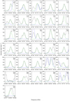Fig. D.1

Selection of CHD₂OH identified lines towards IRAS 16293 A (in black) with the Gaussian fit in green dashed line, with fixed central velocity and FWHM. The same reference spectrum used in the analysis is represented in blue. The squared number in the top-right corner corresponds to the identification number of the transition, i.e. the panel number in Table D.1.

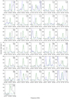Fig. D.2

Selection of CHD₂OH identified lines towards IRAS 16293 B (in black) with the Gaussian fit in green dashed line, with fixed central velocity and FWHM. The same reference spectrum used in the analysis is represented in blue. The squared number in the top-right corner corresponds to the identification number of the transition, i.e. the panel number in Table D.1.

Table D.1

CHD₂OH identified lines.

Appendix E: Synthetic spectra

Figures E.1–E.10 show the synthetic spectra produced by the LTE model using the parameters listed in Tables 1 and 2, for all the detected species. The most unblended and optically thin lines are shown, up to twenty lines for the species having more fitted transitions, such as CH₃OCHO and CH₃COCH₃.

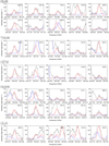Fig. E.1

Representative selection of transitions of CH₃OH isotopologues towards IRAS 16293 A. The synthetic spectra is over-plotted in red, the reference spectrum in blue, and the data in black. The upper energy level of the transition is indicated in the top-left corner.

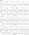Fig. E.2

Representatives selection of transitions of CH₃OCH₃ isotopologues towards IRAS 16293 A. The synthetic spectra is over-plotted in red, the reference spectrum in blue, and the data in black. The upper energy level of the transition is indicated in the top-left corner.

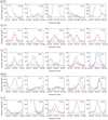Fig. E.3

Representative selection of transitions of H₂CO isotopologues towards IRAS 16293 A. The synthetic spectra is over-plotted in red, the reference spectrum in blue, and the data in black. The dashed curves represent optically thick lines. The upper energy level of the transition is indicated in the top-left corner.

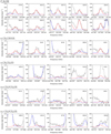Fig. E.4

Representative selection of transitions of C₂H₅OH isotopologues towards IRAS 16293 A. The synthetic spectra is over-plotted in red, the reference spectrum in blue, and the data in black. The upper energy level of the transition is indicated in the top-left corner.

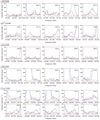Fig. E.5

Representative selection of transitions of t-HCOOH isotopologues and CH₃COOH towards IRAS 16293 A. The synthetic spectra is over-plotted in red, the reference spectrum in blue, and the data in black. The upper energy level of the transition is indicated in the top-left corner.

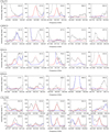Fig. E.6

Representative selection of transitions of CH₂CO and HNCO isotopologues and CH₃CHO towards IRAS 16293 A. The synthetic spectra is over-plotted in red, the reference spectrum in blue, and the data in black. The upper energy level of the transition is indicated in the top-left corner.

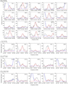Fig. E.7

Representative selection of transitions of CH₃COCH₃, c-H₂ COCH₂, CH₃ O¹³CHO, and CH₂(OH)CHO towards IRAS 16293 A. The synthetic spectra is over-plotted in red, the reference spectrum in blue, and the data in black. The upper energy level of the transition is indicated in the top-left corner.

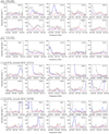Fig. E.8

Representative selection of transitions of the two energetically lowest conformers of (CH₂ OH)₂ towards IRAS 16293 A and t-C₂H₅OCH₃ towards IRAS 16293 A and B. The synthetic spectra is over-plotted in red, the reference spectrum in blue, and the data in black. The upper energy level of the transition is indicated in the top-left corner.

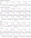Fig. E.9

Representative selection of transitions of CH₃OCH₂OH towards IRAS 16293 A and B and NH₂CHO and C₂H₅CHO towards IRAS 16293 A only. The synthetic spectra is over-plotted in red, the reference spectrum in blue, and the data in black. The upper energy level of the transition is indicated in the top-left corner.

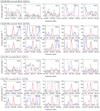Fig. E.10

Representative selection of transitions of CH₂DCHO and CH₃CDO towards IRAS 16293 A and B. The synthetic spectra is over-plotted in red, the reference spectrum in blue, and the data in black. The upper energy level of the transition is indicated in the top-left corner.

References

Altwegg, K., Balsiger, H., Berthelier, J. J., et al. 2017, MNRAS, 469, S130 [Google Scholar]
Andre, P., & Montmerle, T. 1994, ApJ, 420, 837 [NASA ADS] [CrossRef] [Google Scholar]
Astropy Collaboration (Robitaille, T. P., et al.) 2013, A&A, 558, A33 [NASA ADS] [CrossRef] [EDP Sciences] [Google Scholar]
Auwera, J. V. 1992, J. Mol. Spectr., 155, 136 [NASA ADS] [CrossRef] [Google Scholar]
Bacmann, A., Taquet, V., Faure, A., Kahane, C., & Ceccarelli, C. 2012, A&A, 541, L12 [NASA ADS] [CrossRef] [EDP Sciences] [Google Scholar]
Balucani, N., Ceccarelli, C., & Taquet, V. 2015, MNRAS, 449, L16 [Google Scholar]
Baskakov, O. I. 1996, J. Mol. Spectr., 180, 266 [NASA ADS] [CrossRef] [Google Scholar]
Baskakov, O. I., Bürger, H., & Jerzembeck, W. 1999, J. Mol. Spectr., 193, 33 [NASA ADS] [CrossRef] [Google Scholar]
Baskakov, O. I., Alekseev, E. A., Motiyenko, R. A., et al. 2006, J. Mol. Spectr., 240, 188 [NASA ADS] [CrossRef] [Google Scholar]
Bellet, J., Deldalle, A., Samson, C., Stenbeckeliers, G., & Wertheimer, R. 1971, J. Mol. Struct., 9, 65 [NASA ADS] [CrossRef] [Google Scholar]
Belov, S. P., Tretyakov, M. Y., Kleiner, I., & Hougen, J. T. 1993, J. Mol. Spectr., 160, 61 [NASA ADS] [CrossRef] [Google Scholar]
Bergner, J. B., Öberg, K. I., Garrod, R. T., & Graninger, D. M. 2017, ApJ, 841, 120 [NASA ADS] [CrossRef] [Google Scholar]
Bisschop, S. E., Jørgensen, J. K., Bourke, T. L., Bottinelli, S., & van Dishoeck E. F. 2008, A&A, 488, 959 [NASA ADS] [CrossRef] [EDP Sciences] [Google Scholar]
Biver, N., Bockelée-Morvan, D., Debout, V., et al. 2014, A&A, 566, L5 [Google Scholar]
Blake, G. A., Sutton, E. C., Masson, C. R., & Phillips, T. G. 1987, ApJ, 315, 621 [NASA ADS] [CrossRef] [Google Scholar]
Blanco, S., López, J. C., Lesarri, A., & Alonso, J. L. 2006, J. Am. Chem. Soc., 128, 12111 [CrossRef] [Google Scholar]
Bockelée-Morvan, D., Lis, D. C., Wink, J. E., et al. 2000, A&A, 353, 1101 [Google Scholar]
Bocquet, R., Demaison, J., Poteau, L., et al. 1996, J. Mol. Spectr., 177, 154 [NASA ADS] [CrossRef] [Google Scholar]
Bocquet, R., Demaison, J., Cosléou, J., et al. 1999, J. Mol. Spectr., 195, 345 [NASA ADS] [CrossRef] [Google Scholar]
Bøgelund, E. G., Barr, A. G., Taquet, V., et al. 2019, A&A, 628, A2 [NASA ADS] [CrossRef] [EDP Sciences] [Google Scholar]
Botta, O., & Bada, J. L. 2002, Surv. Geophys., 23, 411 [NASA ADS] [CrossRef] [Google Scholar]
Bouchez, A., Walters, A., Müller, H. S. P., et al. 2012, J. Quant. Spectr. Rad. Transf., 113, 1148 [NASA ADS] [CrossRef] [Google Scholar]
Boussessi, R., Senent, M. L., & Jaïdane, N. 2016, J. Chem. Phys., 144, 164110 [NASA ADS] [CrossRef] [Google Scholar]
Brown, R. D., Godfrey, P. D., McNaughton, D., Pierlot, A. P., & Taylor, W. H. 1990, J. Mol. Spectr., 140, 340 [NASA ADS] [CrossRef] [Google Scholar]
Brünken, S., Müller, H. S. P., Lewen, F., & Winnewisser, G. 2003, Phys. Chem. Chem. Phys., 5, 1515 [CrossRef] [Google Scholar]
Burke, D. J., Puletti, F., Brown, W. A., et al. 2015, MNRAS, 447, 1444 [NASA ADS] [CrossRef] [Google Scholar]
Butcher, S. S., & Bright Wilson, Jr., E. 1964, J. Chem. Phys., 40, 1671 [NASA ADS] [CrossRef] [Google Scholar]
Butler, R. A. H., De Lucia, F. C., Petkie, D. T., et al. 2001, ApJS, 134, 319 [NASA ADS] [CrossRef] [Google Scholar]
Calcutt, H., Viti, S., Codella, C., et al. 2014, MNRAS, 443, 3157 [NASA ADS] [CrossRef] [Google Scholar]
Calcutt, H., Fiechter, M. R., Willis, E. R., et al. 2018a, A&A, 617, A95 [NASA ADS] [CrossRef] [EDP Sciences] [Google Scholar]
Calcutt, H., Jørgensen, J. K., Müller, H. S. P., et al. 2018b, A&A, 616, A90 [NASA ADS] [CrossRef] [EDP Sciences] [Google Scholar]
Carroll, P. B., Drouin, B. J., & Widicus Weaver, S. L. 2010, ApJ, 723, 845 [NASA ADS] [CrossRef] [Google Scholar]
Carroll, P. B., McGuire, B. A., Blake, G. A., et al. 2015, ApJ, 799, 15 [NASA ADS] [CrossRef] [Google Scholar]
Carvajal, M., Kleiner, I., & Demaison, J. 2010, ApJS, 190, 315 [NASA ADS] [CrossRef] [Google Scholar]
Caux, E., Kahane, C., Castets, A., et al. 2011, A&A, 532, A23 [NASA ADS] [CrossRef] [EDP Sciences] [Google Scholar]
Cazaux, S., Tielens, A. G. G. M., Ceccarelli, C., et al. 2003, ApJ, 593, L51 [NASA ADS] [CrossRef] [Google Scholar]
Ceccarelli, C., Caselli, P., Fontani, F., et al. 2017, ApJ, 850, 176 [NASA ADS] [CrossRef] [Google Scholar]
Christen, D., & Müller, H. S. P. 2003, Phys. Chem. Chem. Phys., 5, 3600 [CrossRef] [Google Scholar]
Christen, D., Coudert, L. H., Suenram, R. D., & Lovas, F. J. 1995, J. Mol. Spectr., 172, 57 [NASA ADS] [CrossRef] [Google Scholar]
Christen, D., Coudert, L. H., Larsson, J. A., & Cremer, D. 2001, J. Mol. Spectr., 205, 185 [NASA ADS] [CrossRef] [Google Scholar]
Chuang, K.-J., Fedoseev, G., Ioppolo, S., van Dishoeck, E. F., & Linnartz, H. 2016, MNRAS, 455, 1702 [Google Scholar]
Chuang, K.-J., Fedoseev, G., Qasim, D., et al. 2018, ApJ, 853, 102 [NASA ADS] [CrossRef] [Google Scholar]
Cornet, R. A.,& Winnewisser, G. 1980, J. Mol. Spectr., 80, 438 [NASA ADS] [CrossRef] [Google Scholar]
Coudert, L. H., Margulès, L., Vastel, C., et al. 2019, A&A, 624, A70 [NASA ADS] [CrossRef] [EDP Sciences] [Google Scholar]
Coutens, A., Jørgensen, J. K., van der Wiel, M. H. D., et al. 2016, A&A, 590, A1 [NASA ADS] [CrossRef] [EDP Sciences] [Google Scholar]
Coutens, A., Viti, S., Rawlings, J. M. C., et al. 2018, MNRAS, 475, 2016 [NASA ADS] [CrossRef] [Google Scholar]
Coutens, A., Ligterink, N. F. W., Loison, J. C., et al. 2019, A&A, 623, L13 [NASA ADS] [CrossRef] [EDP Sciences] [Google Scholar]
Creswell, R. A., & Schwendeman, R. H. 1974, Chem. Phys. Lett., 27, 521 [NASA ADS] [CrossRef] [Google Scholar]
Crovisier, J., Bockelée-Morvan, D., Biver, N., et al. 2004, A&A, 418, L35 [NASA ADS] [CrossRef] [EDP Sciences] [Google Scholar]
Cunningham, Jr., G. L., Boyd, A. W., Myers, R. J., Gwinn, W. D., & Le van, W. I. 1951, J. Chem. Phys., 19, 676 [NASA ADS] [CrossRef] [Google Scholar]
Dangoisse, D., Willemot, E., & Bellet, J. 1978, J. Mol. Spectr., 71, 414 [NASA ADS] [CrossRef] [Google Scholar]
Demaison, J., Dubrulle, A., Boucher, D., Burie, J., & van Eijck, B. P. 1982, J. Mol. Spectr., 94, 211 [NASA ADS] [CrossRef] [Google Scholar]
Demaison, J., Maes, H., Van Eijck, B. P., Wlodarczak, G., & Lasne, M. C. 1987, J. Mol. Spectr., 125, 214 [NASA ADS] [CrossRef] [Google Scholar]
Drozdovskaya,M. N., Walsh, C., van Dishoeck, E. F., et al. 2016, MNRAS, 462, 977 [NASA ADS] [CrossRef] [Google Scholar]
Drozdovskaya, M. N., van Dishoeck, E. F., Jørgensen, J. K., et al. 2018, MNRAS, 476, 4949 [NASA ADS] [CrossRef] [Google Scholar]
Drozdovskaya, M. N., van Dishoeck, E. F., Rubin, M., Jørgensen, J. K., & Altwegg, K. 2019, MNRAS, 490, 50 [NASA ADS] [CrossRef] [Google Scholar]
Durig, J. R., & Larsen, R. A. 1990, J. Mol. Struct., 238, 195 [NASA ADS] [CrossRef] [Google Scholar]
Durig, J. R., Compton, D. A. C., & McArver, A. Q. 1980, J. Chem. Phys., 73, 719 [NASA ADS] [CrossRef] [Google Scholar]
Durig, J. R., Deeb, H., Darkhalil, I. D., et al. 2011, J. Mol. Struct., 985, 202 [NASA ADS] [CrossRef] [Google Scholar]
Dzib, S. A., Ortiz-León, G. N., Hernández-Gómez, A., et al. 2018, A&A, 614, A20 [NASA ADS] [CrossRef] [EDP Sciences] [Google Scholar]
Ehrenfreund, P., Glavin, D. P., Botta, O., Cooper, G., & Bada, J. L. 2001, Proc. Natl. Acad. Sci., 98, 2138 [NASA ADS] [CrossRef] [Google Scholar]
Elkeurti, M., Coudert, L. H., Medvedev, I. R., et al. 2010, J. Mol. Spectr., 263, 145 [NASA ADS] [CrossRef] [Google Scholar]
Endres, C. P., Drouin, B. J., Pearson, J. C., et al. 2009, A&A, 504, 635 [NASA ADS] [CrossRef] [EDP Sciences] [Google Scholar]
Endres, C. P., Schlemmer, S., Schilke, P., Stutzki, J., & Müller, H. S. P. 2016, J. Mol. Spectr., 327, 95 [NASA ADS] [CrossRef] [Google Scholar]
Fabricant, B., Krieger, D., & Muenter, J. S. 1977, J. Chem. Phys., 67, 1576 [NASA ADS] [CrossRef] [Google Scholar]
Favre, C., Carvajal, M., Field, D., et al. 2014, ApJS, 215, 25 [NASA ADS] [CrossRef] [Google Scholar]
Favre, C., Fedele, D., Semenov, D., et al. 2018, ApJ, 862, L2 [NASA ADS] [CrossRef] [Google Scholar]
Fayolle, E. C., Öberg, K. I., Garrod, R. T., van Dishoeck, E. F., & Bisschop, S. E. 2015, A&A, 576, A45 [NASA ADS] [CrossRef] [EDP Sciences] [Google Scholar]
Fayolle, E. C., Öberg, K. I., Jørgensen, J. K., et al. 2017, Nat. Astron., 1, 703 [NASA ADS] [CrossRef] [Google Scholar]
Fedoseev, G., Cuppen, H. M., Ioppolo, S., Lamberts, T., & Linnartz, H. 2015a, MNRAS, 448, 1288 [NASA ADS] [CrossRef] [Google Scholar]
Fedoseev, G., Ioppolo, S., Zhao, D., Lamberts, T., & Linnartz, H. 2015b, MNRAS, 446, 439 [NASA ADS] [CrossRef] [Google Scholar]
Fedoseev, G., Chuang, K. J., Ioppolo, S., et al. 2017, ApJ, 842, 52 [NASA ADS] [CrossRef] [Google Scholar]
Fisher, J., Paciga, G., Xu, L.-H., et al. 2007, J. Mol. Spectr., 245, 7 [NASA ADS] [CrossRef] [Google Scholar]
Fuchs, U., Winnewisser, G., Groner, P., De Lucia, F. C., & Herbst, E. 2003, ApJS, 144, 277 [NASA ADS] [CrossRef] [Google Scholar]
Fuchs, G. W., Fuchs, U., Giesen, T. F., & Wyrowski, F. 2005, A&A, 444, 521 [NASA ADS] [CrossRef] [EDP Sciences] [Google Scholar]
Fuchs, G. W., Cuppen, H. M., Ioppolo, S., et al. 2009, A&A, 505, 629 [NASA ADS] [CrossRef] [EDP Sciences] [Google Scholar]
Gardner, F. F., Godfrey, P. D., & Williams, D. R. 1980, MNRAS, 193, 713 [NASA ADS] [CrossRef] [Google Scholar]
Garrod, R. T. 2013, ApJ, 765, 60 [Google Scholar]
Garrod, R. T.,& Herbst, E. 2006, A&A, 457, 927 [NASA ADS] [CrossRef] [EDP Sciences] [Google Scholar]
Garrod, R. T., Widicus Weaver, S. L., & Herbst, E. 2008, ApJ, 682, 283 [NASA ADS] [CrossRef] [Google Scholar]
Girart, J. M., Estalella, R., Palau, A., Torrelles, J. M., & Rao, R. 2014, ApJ, 780, L11 [NASA ADS] [CrossRef] [Google Scholar]
Groner, P., Albert, S., Herbst, E., & De Lucia, F. C. 1998, ApJ, 500, 1059 [NASA ADS] [CrossRef] [Google Scholar]
Groner, P., Albert, S., Herbst, E., et al. 2002, ApJS, 142, 145 [NASA ADS] [CrossRef] [Google Scholar]
Groner, P., Herbst, E., De Lucia, F. C., Drouin, B. J., & Mäder, H. 2006, J. Mol. Struct., 795, 173 [NASA ADS] [CrossRef] [Google Scholar]
Guarnieri, A. 2005, Z. Naturforsch. A, 60, 619 [NASA ADS] [CrossRef] [Google Scholar]
Guarnieri, A., & Huckaufa, A. 2003, Z. Naturforsch. A, 58, 275 [NASA ADS] [CrossRef] [Google Scholar]
Hardy, J. A., Cox, A. P., Fliege, E., & Dreizler, H. 1982, Z. Naturforsch. A, 37, 1035 [NASA ADS] [CrossRef] [Google Scholar]
Hayashi, M., & Adachi, M. 1982, J. Mol. Struct., 78, 53 [NASA ADS] [CrossRef] [Google Scholar]
Hayashi, M., & Kuwada, K. 1975, J. Mol. Struct., 28, 147 [NASA ADS] [CrossRef] [Google Scholar]
Hays, B. M., & Widicus Weaver, S. L. 2013, J. Phys. Chem. A, 117, 7142 [NASA ADS] [CrossRef] [Google Scholar]
Herbst, E., & van Dishoeck, E. F. 2009, ARA&A, 47, 427 [NASA ADS] [CrossRef] [Google Scholar]
Hirose, C. 1974, ApJ, 189, L145 [NASA ADS] [CrossRef] [Google Scholar]
Hirota, E., Sugisaki, R., Nielsen, C. J., & Sørensen, G. O. 1974, J. Mol. Spectr., 49, 251 [NASA ADS] [CrossRef] [Google Scholar]
Hocking, W. H., Gerry, M. C. L., & Winnewisser, G. 1975, Can. J. Phys., 53, 1869 [NASA ADS] [CrossRef] [Google Scholar]
Hollis, J. M., Vogel, S. N., Snyder, L. E., Jewell, P. R., & Lovas, F. J. 2001, ApJ, 554, L81 [Google Scholar]
Hunter, J. D. 2007, Comput. Sci. Eng., 9, 90 [NASA ADS] [CrossRef] [Google Scholar]
Ikeda, M., Duan, Y.-B., Tsunekawa, S., & Takagi, K. 1998, ApJS, 117, 249 [NASA ADS] [CrossRef] [Google Scholar]
Ilyushin, V. V., Alekseev, E. A., Dyubko, S. F., et al. 2001, J. Mol. Spectr., 205, 286 [NASA ADS] [CrossRef] [Google Scholar]
Ilyushin, V. V., Alekseev, E. A., Dyubko, S. F., & Kleiner, I. 2003, J. Mol. Spectr., 220, 170 [NASA ADS] [CrossRef] [Google Scholar]
Ilyushin, V., Kleiner, I., & Lovas, F. J. 2008, J. Phys. Chem. Ref. Data, 37, 97 [NASA ADS] [CrossRef] [Google Scholar]
Ilyushin, V. V., Endres, C. P., Lewen, F., Schlemmer, S., & Drouin, B. J. 2013, J. Mol. Spectr., 290, 31 [NASA ADS] [CrossRef] [Google Scholar]
Jacobsen, S. K., Jørgensen, J. K., van der Wiel, M. H. D., et al. 2018, A&A, 612, A72 [NASA ADS] [CrossRef] [EDP Sciences] [Google Scholar]
Johns, J. W. C., & McKellar, A. R. W. 1977, J. Mol. Spectr., 64, 327 [NASA ADS] [CrossRef] [Google Scholar]
Johns, J. W. C., Nemes, L., Yamada, K. M. T., et al. 1992, J. Mol. Spectr., 156, 501 [NASA ADS] [CrossRef] [Google Scholar]
Johnson, H. R., & Strandberg, M. W. P. 1952, J. Chem. Phys., 20, 687 [NASA ADS] [CrossRef] [Google Scholar]
Jones, E., Oliphant, T., Peterson, P., et al. 2001, SciPy: Open source scientific tools for Python [Google Scholar]
Jørgensen, J. K., Bourke, T. L., Nguyen Luong, Q., & Takakuwa, S. 2011, A&A, 534, A100 [NASA ADS] [CrossRef] [EDP Sciences] [Google Scholar]
Jørgensen, J. K., Favre, C., Bisschop, S. E., et al. 2012, ApJ, 757, L4 [NASA ADS] [CrossRef] [Google Scholar]
Jørgensen, J. K., van der Wiel, M. H. D., Coutens, A., et al. 2016, A&A, 595, A117 [NASA ADS] [CrossRef] [EDP Sciences] [Google Scholar]
Jørgensen, J. K., Müller, H. S. P., Calcutt, H., et al. 2018, A&A, 620, A170 [NASA ADS] [CrossRef] [EDP Sciences] [Google Scholar]
Kleiner, I., Lovas, F. J., & Godefroid, M. 1996, J. Phys. Chem. Ref. Data, 25, 1113 [CrossRef] [Google Scholar]
Kobayashi, K., Sakai, Y., Tsunekawa, S., et al. 2016, J. Mol. Spectr., 321, 63 [NASA ADS] [CrossRef] [Google Scholar]
Koerber, M., Bisschop, S. E., Endres, C. P., et al. 2013, A&A, 558, A112 [NASA ADS] [CrossRef] [EDP Sciences] [Google Scholar]
Krisher, L. C.,& Saegebarth, E. 1971, J. Chem. Phys., 54, 4553 [NASA ADS] [CrossRef] [Google Scholar]
Kryvda, A. V., Gerasimov, V. G., Dyubko, S. F., Alekseev, E. A., & Motiyenko, R. A. 2009, J. Mol. Spectr., 254, 28 [NASA ADS] [CrossRef] [Google Scholar]
Kukolich, S. G., & Nelson, A. C. 1971, Chem. Phys. Lett., 11, 383 [NASA ADS] [CrossRef] [Google Scholar]
Kurland, R. J., & Bright Wilson, Jr., E. 1957, J. Chem. Phys., 27, 585 [NASA ADS] [CrossRef] [Google Scholar]
Kuze, H., Kuga, T., & Shimizu, T. 1982, J. Mol. Spectr., 93, 248 [Google Scholar]
Lapinov, A. V., Golubiatnikov, G. Y., Markov, V. N., & Guarnieri, A. 2007, Astron. Lett., 33, 121 [NASA ADS] [CrossRef] [Google Scholar]
Lattanzi, V., Walters, A., Drouin, B. J., & Pearson, J. C. 2008, ApJS, 176, 536 [NASA ADS] [CrossRef] [Google Scholar]
Le Roy, L., Altwegg, K., Balsiger, H., et al. 2015, A&A, 583, A1 [NASA ADS] [CrossRef] [EDP Sciences] [Google Scholar]
Lerner, R. G., Dailey, B. P., & Friend, J. P. 1957, J. Chem. Phys., 26, 680 [NASA ADS] [CrossRef] [Google Scholar]
Li, J., Shen, Z., Wang, J., et al. 2017, ApJ, 849, 115 [NASA ADS] [CrossRef] [Google Scholar]
Ligterink, N. F. W., Coutens, A., Kofman, V., et al. 2017, MNRAS, 469, 2219 [NASA ADS] [CrossRef] [Google Scholar]
Lohilahti, J., & Horneman, V.-M. 2004, J. Mol. Spectr., 228, 1 [NASA ADS] [CrossRef] [Google Scholar]
López-Sepulcre, A., Sakai, N., Neri, R., et al. 2017, A&A, 606, A121 [NASA ADS] [CrossRef] [EDP Sciences] [Google Scholar]
Lykke, J. M., Coutens, A., Jørgensen, J. K., et al. 2017, A&A, 597, A53 [NASA ADS] [CrossRef] [EDP Sciences] [Google Scholar]
Maeda, A., Medvedev, I. R., De Lucia, F. C., Herbst, E., & Groner, P. 2008a, ApJS, 175, 138 [NASA ADS] [CrossRef] [Google Scholar]
Maeda, A., De Lucia, F. C., & Herbst, E. 2008b, J. Mol. Spectr., 251, 293 [NASA ADS] [CrossRef] [Google Scholar]
Manigand, S., Calcutt, H., Jørgensen, J. K., et al. 2019, A&A, 623, A69 [NASA ADS] [CrossRef] [EDP Sciences] [Google Scholar]
Marstokk, K.-M., & Møllendal, H. 1970, J. Mol. Struct., 5, 205 [NASA ADS] [CrossRef] [Google Scholar]
Marstokk, K.-M., & Møllendal, H. 1973, J. Mol. Struct., 16, 259 [NASA ADS] [CrossRef] [Google Scholar]
Martinache, L., & Bauder, A. 1989, Chem. Phys. Lett., 164, 657 [NASA ADS] [CrossRef] [Google Scholar]
McGuire, B. A., Shingledecker, C. N., Willis, E. R., et al. 2017, ApJ, 851, L46 [NASA ADS] [CrossRef] [Google Scholar]
McMullin, J. P., Waters, B., Schiebel, D., Young, W., & Golap, K. 2007, ASP Conf. Ser., 376, 127 [Google Scholar]
Medcraft, C., Thompson, C. D., Robertson, E. G., Appadoo, D. R. T., & McNaughton, D. 2012, ApJ, 753, 18 [NASA ADS] [CrossRef] [Google Scholar]
Milam, S. N., Savage, C., Brewster, M. A., Ziurys, L. M., & Wyckoff, S. 2005, ApJ, 634, 1126 [NASA ADS] [CrossRef] [Google Scholar]
Mollabashi, M., Lees, R. M., Xu, L.-H., & Bakota, M. 1993, Int. J. Infrared Millim. Waves, 14, 2569 [NASA ADS] [CrossRef] [Google Scholar]
Morina, L., Obst, S., Unrath, M., et al. 2019, J. Mol. Spectr., 356, 1 [NASA ADS] [CrossRef] [Google Scholar]
Moskienko, E. M., & Dyubko, S. F. 1991, Radiophys. Quant. Electron., 34, 181 [NASA ADS] [CrossRef] [Google Scholar]
Motiyenko, R. A., Tercero, B., Cernicharo, J., & Margulès, L. 2012, A&A, 548, A71 [NASA ADS] [CrossRef] [EDP Sciences] [Google Scholar]
Motiyenko, R. A., Margulès, L., Despois, D., & Guillemin, J.-C. 2018, Phys. Chem. Chem. Phys., 20, 5509 [NASA ADS] [CrossRef] [Google Scholar]
Mukhopadhyay, I. 2016, Infrared Phys. Technol., 75, 139 [NASA ADS] [CrossRef] [Google Scholar]
Müller, H. S. P., & Christen, D. 2004, J. Mol. Spectr., 228, 298 [NASA ADS] [CrossRef] [Google Scholar]
Müller, H. S. P., & Lewen, F. 2017, J. Mol. Spectr., 331, 28 [NASA ADS] [CrossRef] [Google Scholar]
Müller, H. S. P., Gendriesch, R., Margulès, L., et al. 2000a, Phys. Chem. Chem. Phys., 2, 3401 [CrossRef] [Google Scholar]
Müller, H. S. P., Gendriesch, R., Lewen, F., & Winnewisser, G. 2000b, Z. Naturforsch. A, 55 [Google Scholar]
Müller, H. S. P., Winnewisser, G., Demaison, J., Perrin, A., & Valentin, A. 2000c, J. Mol. Spectr., 200, 143 [NASA ADS] [CrossRef] [Google Scholar]
Müller, H. S. P., Thorwirth, S., Roth, D. A., & Winnewisser, G. 2001, A&A, 370, L49 [NASA ADS] [CrossRef] [EDP Sciences] [Google Scholar]
Müller, H. S. P., Schlöder, F., Stutzki, J., & Winnewisser, G. 2005, J. Mol. Struct., 742, 215 [NASA ADS] [CrossRef] [Google Scholar]
Müller, H. S. P., Xu, L.-H., & van der Tak, F. 2006, J. Mol. Struct., 795, 114 [NASA ADS] [CrossRef] [Google Scholar]
Müller, H. S. P., Belloche, A., Xu, L.-H., et al. 2016, A&A, 587, A92 [NASA ADS] [CrossRef] [EDP Sciences] [Google Scholar]
Ndao, M., Kwabia Tchana, F., Coudert, L. H., et al. 2016, J. Mol. Spectr., 326, 136 [NASA ADS] [CrossRef] [Google Scholar]
Niedenhoff, M., Yamada, K. M. T., Belov, S. P., & Winnewisser, G. 1995, J. Mol. Spectr., 174, 151 [NASA ADS] [CrossRef] [Google Scholar]
Nielsen, C. J. 1973, PhD thesis, Københavns Universitet, Denmark [Google Scholar]
Öberg, K. I., Garrod, R. T., van Dishoeck, E. F., & Linnartz, H. 2009, A&A, 504, 891 [NASA ADS] [CrossRef] [EDP Sciences] [Google Scholar]
Öberg, K. I., Furuya, K., Loomis, R., et al. 2015, ApJ, 810, 112 [NASA ADS] [CrossRef] [Google Scholar]
Ochsenbein, F., Bauer, P., & Marcout, J. 2000, A&AS, 143, 23 [NASA ADS] [CrossRef] [EDP Sciences] [Google Scholar]
Oldag, F., & Sutter, D. H. 1992, Z. Naturforsch. A, 47, 527 [NASA ADS] [CrossRef] [Google Scholar]
Ordu, M. H., Zingsheim, O., Belloche, A., et al. 2019, A&A, 629, A72 [NASA ADS] [CrossRef] [EDP Sciences] [Google Scholar]
Ospina-Zamudio, J., Lefloch, B., Ceccarelli, C., et al. 2018, A&A, 618, A145 [NASA ADS] [CrossRef] [EDP Sciences] [Google Scholar]
Oya, Y., Sakai, N., López-Sepulcre, A., et al. 2016, ApJ, 824, 88 [NASA ADS] [CrossRef] [Google Scholar]
Paardekooper,D. M., Bossa, J. B., & Linnartz, H. 2016, A&A, 592, A67 [NASA ADS] [CrossRef] [EDP Sciences] [Google Scholar]
Pan, J., Albert, S., Sastry, K. V. L. N., Herbst, E., & De Lucia, F. C. 1998, ApJ, 499, 517 [NASA ADS] [CrossRef] [Google Scholar]
Parise, B., Ceccarelli, C., Tielens, A. G. G. M., et al. 2002, A&A, 393, L49 [NASA ADS] [CrossRef] [EDP Sciences] [Google Scholar]
Parise, B., Castets, A., Herbst, E., et al. 2004, A&A, 416, 159 [NASA ADS] [CrossRef] [EDP Sciences] [Google Scholar]
Pearson, J. C., Sastry, K. V. L. N., Winnewisser, M., Herbst, E., & De Lucia, F. C. 1995, J. Phys. Chem. Ref. Data, 24, 1 [NASA ADS] [CrossRef] [Google Scholar]
Pearson, J. C., Sastry, K. V. L. N., Herbst, E., & De Lucia, F. C. 1996, J. Mol. Spectr., 175, 246 [NASA ADS] [CrossRef] [Google Scholar]
Pearson, J. C., Brauer, C. S., & Drouin, B. J. 2008, J. Mol. Spectr., 251, 394 [NASA ADS] [CrossRef] [Google Scholar]
Pearson, J. C., Yu, S., & Drouin, B. J. 2012, J. Mol. Spectr., 280, 119 [NASA ADS] [CrossRef] [Google Scholar]
Penzias, A. A. 1981, ApJ, 249, 518 [NASA ADS] [CrossRef] [Google Scholar]
Persson, M. V., Jørgensen, J. K., & van Dishoeck, E. F. 2012, A&A, 541, A39 [NASA ADS] [CrossRef] [EDP Sciences] [Google Scholar]
Persson, M. V., Jørgensen, J. K., Müller, H. S. P., et al. 2018, A&A, 610, A54 [NASA ADS] [CrossRef] [EDP Sciences] [Google Scholar]
Peter, R., & Dreizler, H. 1965, Z. Naturforsch. A, 20, 301 [NASA ADS] [Google Scholar]
Pickett, H. M., Poynter, R. L., Cohen, E. A., et al. 1998, J. Quant. Spectr. Rad. Transf., 60, 883 [NASA ADS] [CrossRef] [Google Scholar]
Pineda, J. E., Maury, A. J., Fuller, G. A., et al. 2012, A&A, 544, L7 [NASA ADS] [CrossRef] [EDP Sciences] [Google Scholar]
Potin, S., Manigand, S., Beck, P., Wolters, C., & Schmitt, B. 2019, Icarus, submitted [Google Scholar]
Qasim, D., Fedoseev, G., Chuang, K. J., et al. 2019a, A&A, 627, A1 [NASA ADS] [CrossRef] [EDP Sciences] [Google Scholar]
Qasim, D., Lamberts, T., He, J., et al. 2019b, A&A, 626, A118 [NASA ADS] [CrossRef] [EDP Sciences] [Google Scholar]
Richard, C., Margulès, L., Caux, E., et al. 2013, A&A, 552, A117 [NASA ADS] [CrossRef] [EDP Sciences] [Google Scholar]
Senent, M., Ruiz, R., Villa, M., & Domínguez-Gómez, R. 2009, J. Chem. Phys., 130, 064101 [NASA ADS] [CrossRef] [Google Scholar]
Skouteris, D., Vazart, F., Ceccarelli, C., et al. 2017, MNRAS, 468, L1 [NASA ADS] [Google Scholar]
Skouteris, D., Balucani, N., Ceccarelli, C., et al. 2018, ApJ, 854, 135 [Google Scholar]
Skouteris, D., Balucani, N., Ceccarelli, C., et al. 2019, MNRAS, 482, 3567 [NASA ADS] [CrossRef] [Google Scholar]
Sutter, D. H., & Dreizler, H. 2000, Z. Naturforsch. A, 55, 695 [NASA ADS] [CrossRef] [Google Scholar]
Tabor, W. J. 1957, J. Chem. Phys., 27, 974 [NASA ADS] [CrossRef] [Google Scholar]
Taquet, V., Wirström, E. S., Charnley, S. B., et al. 2017, A&A, 607, A20 [NASA ADS] [CrossRef] [EDP Sciences] [Google Scholar]
Tercero, B., Cernicharo, J., López, A., et al. 2015, A&A, 582, L1 [NASA ADS] [CrossRef] [EDP Sciences] [Google Scholar]
Tercero, B., Cuadrado, S., López, A., et al. 2018, A&A, 620, L6 [NASA ADS] [CrossRef] [EDP Sciences] [Google Scholar]
Tsunekawa, S., Kinai, Y., Kondo, Y., Odashima, H., & Takagi, K. 2003, Molecules, 8, 103 [CrossRef] [Google Scholar]
Tsunekawa, S., Kinai, Y., Kondo, Y., et al. 2011, Toyama Univ. Mol. Spectr. Data, 4 [Google Scholar]
Turner, P. H., & Cox, A. P. 1976, Chem. Phys. Lett., 42, 84 [NASA ADS] [CrossRef] [Google Scholar]
Turner, P. H., Cox, A. P., & Hardy, J. A. 1981, J. Chem. Soc. Faraday Trans. 2, 77, 1217 [CrossRef] [Google Scholar]
Vacherand, J. M., Van Eijck, B. P., Burie, J., & Demaison, J. 1986, J. Mol. Spectr., 118, 355 [NASA ADS] [CrossRef] [Google Scholar]
van der Walt, S., Colbert, S. C., & Varoquaux, G. 2011, Comput. Sci. Eng., 13, 22 [Google Scholar]
van der Wiel, M. H. D., Jacobsen, S. K., Jørgensen, J. K., et al. 2019, A&A, 626, A93 [NASA ADS] [CrossRef] [EDP Sciences] [Google Scholar]
van Dishoeck, E. F., Blake, G. A., Jansen, D. J., & Groesbeck, T. D. 1995, ApJ, 447, 760 [NASA ADS] [CrossRef] [Google Scholar]
van Eijck, B. P., van Opheusden, J., van Schaik, M. M. M., & van Zoeren, E. 1981, J. Mol. Spectr., 86, 465 [NASA ADS] [CrossRef] [Google Scholar]
van Eijck, B. P., & van Duijneveldt, F. B. 1983, J. Mol. Spectr., 102, 273 [NASA ADS] [CrossRef] [Google Scholar]
Vorob’eva, E. M., & Dyubko, S. F. 1994, Radiophys. Quantum Electron., 37, 155 [NASA ADS] [CrossRef] [Google Scholar]
Walsh, M. S., Xu, L.-H., & Lees, R. M. 1998, J. Mol. Spectr., 188, 85 [NASA ADS] [CrossRef] [Google Scholar]
Walsh, C., Juhász, A., Meeus, G., et al. 2016, ApJ, 831, 200 [NASA ADS] [CrossRef] [Google Scholar]
Walters, A., Schäfer, M., Ordu, M. H., et al. 2015, J. Mol. Spectr., 314, 6 [NASA ADS] [CrossRef] [Google Scholar]
Wellington Davis, R., Robiette, A. G., Gerry, M. C. L., Bjarnov, E., & Winnemisser, G. 1980, J. Mol. Spectr., 81, 93 [NASA ADS] [CrossRef] [Google Scholar]
Widicus Weaver, S. L., Butler, R. A. H., Drouin, B. J., et al. 2005, ApJS, 158, 188 [NASA ADS] [CrossRef] [Google Scholar]
Willaert, F., Møllendal, H., Alekseev, E., et al. 2006, J. Mol. Struct., 795, 4 [NASA ADS] [CrossRef] [Google Scholar]
Willemot, E., Dangoisse, D., Monnanteuil, N., & Bellet, J. 1980, J. Phys. Chem. Ref. Data, 9, 59 [NASA ADS] [CrossRef] [Google Scholar]
Wilson, T. L. 1999, Rep. Prog. Phys., 62, 143 [Google Scholar]
Winnewisser, M., Winnewisser, B. P., Stein, M., et al. 2002, J. Mol. Spectr., 216, 259 [NASA ADS] [CrossRef] [Google Scholar]
Wlodarczak, G., & Demaison, J. 1988, A&A, 192, 313 [NASA ADS] [Google Scholar]
Xu, L.-H., & Lovas, F. J. 1997, J. Phys. Chem. Ref. Data, 26, 17 [NASA ADS] [CrossRef] [Google Scholar]
Xu, L.-H., Walsh, M. S., & Lees, R. M. 1996, J. Mol. Spectr., 179, 269 [NASA ADS] [CrossRef] [Google Scholar]
Xu, L. H., Müller, H. S. P., van der Tak, F. F. S., & Thorwirth, S. 2004, J. Mol. Spectr., 228, 220 [NASA ADS] [CrossRef] [Google Scholar]
Xue, C., Remijan, A. J., Burkhardt, A. M., & Herbst, E. 2019, ApJ, 871, 112 [NASA ADS] [CrossRef] [Google Scholar]
Zakharenko, O., Motiyenko, R. A., Margulès, L., & Huet, T. R. 2015, J. Mol. Spectr., 317, 41 [Google Scholar]
Zingsheim, O., Müller, H. S. P., Lewen, F., Jørgensen, J. K., & Schlemmer, S. 2017, J. Mol. Spectr., 342, 125 [NASA ADS] [CrossRef] [Google Scholar]

¹

The reduced dataset and all the publications are available on the website http://youngstars.nbi.dk/PILS/.

²

https://cdms.astro.uni-koeln.de/

³

https://spec.jpl.nasa.gov/

⁴

http://cdsarc.u-strasbg.fr/

⁵

It is the combination of four torsional transitions at 244.4 and 231.1 cm⁻¹ of the trans conformer and 490.0 and 453.0 cm⁻¹ of the gauche conformer.

All Tables

Table 1

Best-fit results of all the detected and tentatively detected species towards IRAS 16293 A.

In the text

Table 2

Rotational temperature, column density, and relative abundance with respect to CH₃ OH for the newlydetected species.

In the text

Table D.1

CHD₂OH identified lines.

In the text

All Figures

	Fig. 1 Portion of the spectrum towards IRAS 16293 A and IRAS 16293 B in red and blue, respectively, extracted on their corresponding offset positions. IRAS 16293 A spectrum is offset by 0.5 Jy beam⁻¹ for illustrative purposes.
In the text

Fig. 2

Relative abundances of the main isotopologues with respect to CH₃OH, towards IRAS 16293 A in red and IRAS 16293 B in blue. The abundances towards IRAS 16293 B are based on Persson et al. (2018) for H₂ CO, Lykke et al. (2017) for CH₃CHO, c-H₂ COCH₂, and CH₃ COCH₃, Jørgensen et al. (2016) for CH₂(OH)CHO and CH₃ COOH, and Jørgensen et al. (2018) for CH₂CO, CH₃ OCH₃, C₂ H₅OH, CH₃ OCHO, (CH₂ OH)₂, and t-HCOOH. We note that 30 and 10% of the uncertainties on the column density are considered for IRAS 16293 A and IRAS 16293 B, respectively.

In the text

Fig. 3

Left: cross-comparison of species from IRAS 16293 A in comparison to those from IRAS 16293 B. The statistical distance S is represented in the colour scale for each pair of species. One cell with a given value S of the plot should be read as “The abundance of the species X with respect to Y towards IRAS 16293 A is S sigma higheror lower compared to IRAS 16293 B”, with X and Y species taken from the X-axis and Y -axis, respectively. A positive value of S corresponds to N_X∕N_Y higher in IRAS 16293 A in comparison to IRAS 16293 B. Right: “CH₃OH” and “C₂ H₅OH” rows of the cross-comparison map. The two plots show the comparison of abundances with respect to CH₃ OH (upper panel) and C₂H₅OH (lower panel) towards IRAS 16293 A and IRAS 16293 B in terms of statistical distance.

In the text

	Fig. 4 Representative velocity integrated emission maps of the detected COMs towards IRAS 16293 A. The black and white crosses indicate the continuum peak position and the offset position, respectively. The species and the line frequency are noted in the top-left corner and the 0.′′ 5 beam is shown in the bottom right corner of each panels.
In the text

Fig. 5

D/H ratio of the deuterated species detected towards IRAS 16293 A in red and IRAS 16293 B in blue. The D/H ratio is calculated from the abundance ratio, with the statistical correction due to the chemical group (see Appendix B of Manigand et al. 2019). D/H ratios towards IRAS 16293 B are taken from Coutens et al. (2016), Lykke et al. (2017), Persson et al. (2018), and Jørgensen et al. (2018).

In the text

	Fig. D.1 Selection of CHD₂OH identified lines towards IRAS 16293 A (in black) with the Gaussian fit in green dashed line, with fixed central velocity and FWHM. The same reference spectrum used in the analysis is represented in blue. The squared number in the top-right corner corresponds to the identification number of the transition, i.e. the panel number in Table D.1.
In the text

	Fig. D.2 Selection of CHD₂OH identified lines towards IRAS 16293 B (in black) with the Gaussian fit in green dashed line, with fixed central velocity and FWHM. The same reference spectrum used in the analysis is represented in blue. The squared number in the top-right corner corresponds to the identification number of the transition, i.e. the panel number in Table D.1.
In the text

	Fig. E.1 Representative selection of transitions of CH₃OH isotopologues towards IRAS 16293 A. The synthetic spectra is over-plotted in red, the reference spectrum in blue, and the data in black. The upper energy level of the transition is indicated in the top-left corner.
In the text

	Fig. E.2 Representatives selection of transitions of CH₃OCH₃ isotopologues towards IRAS 16293 A. The synthetic spectra is over-plotted in red, the reference spectrum in blue, and the data in black. The upper energy level of the transition is indicated in the top-left corner.
In the text

	Fig. E.3 Representative selection of transitions of H₂CO isotopologues towards IRAS 16293 A. The synthetic spectra is over-plotted in red, the reference spectrum in blue, and the data in black. The dashed curves represent optically thick lines. The upper energy level of the transition is indicated in the top-left corner.
In the text

	Fig. E.4 Representative selection of transitions of C₂H₅OH isotopologues towards IRAS 16293 A. The synthetic spectra is over-plotted in red, the reference spectrum in blue, and the data in black. The upper energy level of the transition is indicated in the top-left corner.
In the text

	Fig. E.5 Representative selection of transitions of t-HCOOH isotopologues and CH₃COOH towards IRAS 16293 A. The synthetic spectra is over-plotted in red, the reference spectrum in blue, and the data in black. The upper energy level of the transition is indicated in the top-left corner.
In the text

	Fig. E.6 Representative selection of transitions of CH₂CO and HNCO isotopologues and CH₃CHO towards IRAS 16293 A. The synthetic spectra is over-plotted in red, the reference spectrum in blue, and the data in black. The upper energy level of the transition is indicated in the top-left corner.
In the text

	Fig. E.7 Representative selection of transitions of CH₃COCH₃, c-H₂ COCH₂, CH₃ O¹³CHO, and CH₂(OH)CHO towards IRAS 16293 A. The synthetic spectra is over-plotted in red, the reference spectrum in blue, and the data in black. The upper energy level of the transition is indicated in the top-left corner.
In the text

	Fig. E.8 Representative selection of transitions of the two energetically lowest conformers of (CH₂ OH)₂ towards IRAS 16293 A and t-C₂H₅OCH₃ towards IRAS 16293 A and B. The synthetic spectra is over-plotted in red, the reference spectrum in blue, and the data in black. The upper energy level of the transition is indicated in the top-left corner.
In the text

	Fig. E.9 Representative selection of transitions of CH₃OCH₂OH towards IRAS 16293 A and B and NH₂CHO and C₂H₅CHO towards IRAS 16293 A only. The synthetic spectra is over-plotted in red, the reference spectrum in blue, and the data in black. The upper energy level of the transition is indicated in the top-left corner.
In the text

	Fig. E.10 Representative selection of transitions of CH₂DCHO and CH₃CDO towards IRAS 16293 A and B. The synthetic spectra is over-plotted in red, the reference spectrum in blue, and the data in black. The upper energy level of the transition is indicated in the top-left corner.
In the text

Current usage metrics show cumulative count of Article Views (full-text article views including HTML views, PDF and ePub downloads, according to the available data) and Abstracts Views on Vision4Press platform.

Data correspond to usage on the plateform after 2015. The current usage metrics is available 48-96 hours after online publication and is updated daily on week days.

Initial download of the metrics may take a while.

[1] Altwegg, K., Balsiger, H., Berthelier, J. J., et al. 2017, MNRAS, 469, S130 [Google Scholar]

[2] Andre, P., & Montmerle, T. 1994, ApJ, 420, 837 [NASA ADS] [CrossRef] [Google Scholar]

[3] Astropy Collaboration (Robitaille, T. P., et al.) 2013, A&A, 558, A33 [NASA ADS] [CrossRef] [EDP Sciences] [Google Scholar]

[4] Auwera, J. V. 1992, J. Mol. Spectr., 155, 136 [NASA ADS] [CrossRef] [Google Scholar]

[5] Bacmann, A., Taquet, V., Faure, A., Kahane, C., & Ceccarelli, C. 2012, A&A, 541, L12 [NASA ADS] [CrossRef] [EDP Sciences] [Google Scholar]

[6] Balucani, N., Ceccarelli, C., & Taquet, V. 2015, MNRAS, 449, L16 [Google Scholar]

[7] Baskakov, O. I. 1996, J. Mol. Spectr., 180, 266 [NASA ADS] [CrossRef] [Google Scholar]

[8] Baskakov, O. I., Bürger, H., & Jerzembeck, W. 1999, J. Mol. Spectr., 193, 33 [NASA ADS] [CrossRef] [Google Scholar]

[9] Baskakov, O. I., Alekseev, E. A., Motiyenko, R. A., et al. 2006, J. Mol. Spectr., 240, 188 [NASA ADS] [CrossRef] [Google Scholar]

[10] Bellet, J., Deldalle, A., Samson, C., Stenbeckeliers, G., & Wertheimer, R. 1971, J. Mol. Struct., 9, 65 [NASA ADS] [CrossRef] [Google Scholar]

[11] Belov, S. P., Tretyakov, M. Y., Kleiner, I., & Hougen, J. T. 1993, J. Mol. Spectr., 160, 61 [NASA ADS] [CrossRef] [Google Scholar]

[12] Bergner, J. B., Öberg, K. I., Garrod, R. T., & Graninger, D. M. 2017, ApJ, 841, 120 [NASA ADS] [CrossRef] [Google Scholar]

[13] Bisschop, S. E., Jørgensen, J. K., Bourke, T. L., Bottinelli, S., & van Dishoeck E. F. 2008, A&A, 488, 959 [NASA ADS] [CrossRef] [EDP Sciences] [Google Scholar]

[14] Biver, N., Bockelée-Morvan, D., Debout, V., et al. 2014, A&A, 566, L5 [Google Scholar]

[15] Blake, G. A., Sutton, E. C., Masson, C. R., & Phillips, T. G. 1987, ApJ, 315, 621 [NASA ADS] [CrossRef] [Google Scholar]

[16] Blanco, S., López, J. C., Lesarri, A., & Alonso, J. L. 2006, J. Am. Chem. Soc., 128, 12111 [CrossRef] [Google Scholar]

[17] Bockelée-Morvan, D., Lis, D. C., Wink, J. E., et al. 2000, A&A, 353, 1101 [Google Scholar]

[18] Bocquet, R., Demaison, J., Poteau, L., et al. 1996, J. Mol. Spectr., 177, 154 [NASA ADS] [CrossRef] [Google Scholar]

[19] Bocquet, R., Demaison, J., Cosléou, J., et al. 1999, J. Mol. Spectr., 195, 345 [NASA ADS] [CrossRef] [Google Scholar]

[20] Bøgelund, E. G., Barr, A. G., Taquet, V., et al. 2019, A&A, 628, A2 [NASA ADS] [CrossRef] [EDP Sciences] [Google Scholar]

[21] Botta, O., & Bada, J. L. 2002, Surv. Geophys., 23, 411 [NASA ADS] [CrossRef] [Google Scholar]

[22] Bouchez, A., Walters, A., Müller, H. S. P., et al. 2012, J. Quant. Spectr. Rad. Transf., 113, 1148 [NASA ADS] [CrossRef] [Google Scholar]

[23] Boussessi, R., Senent, M. L., & Jaïdane, N. 2016, J. Chem. Phys., 144, 164110 [NASA ADS] [CrossRef] [Google Scholar]

[24] Brown, R. D., Godfrey, P. D., McNaughton, D., Pierlot, A. P., & Taylor, W. H. 1990, J. Mol. Spectr., 140, 340 [NASA ADS] [CrossRef] [Google Scholar]

[25] Brünken, S., Müller, H. S. P., Lewen, F., & Winnewisser, G. 2003, Phys. Chem. Chem. Phys., 5, 1515 [CrossRef] [Google Scholar]

[26] Burke, D. J., Puletti, F., Brown, W. A., et al. 2015, MNRAS, 447, 1444 [NASA ADS] [CrossRef] [Google Scholar]

[27] Butcher, S. S., & Bright Wilson, Jr., E. 1964, J. Chem. Phys., 40, 1671 [NASA ADS] [CrossRef] [Google Scholar]

[28] Butler, R. A. H., De Lucia, F. C., Petkie, D. T., et al. 2001, ApJS, 134, 319 [NASA ADS] [CrossRef] [Google Scholar]

[29] Calcutt, H., Viti, S., Codella, C., et al. 2014, MNRAS, 443, 3157 [NASA ADS] [CrossRef] [Google Scholar]

[30] Calcutt, H., Fiechter, M. R., Willis, E. R., et al. 2018a, A&A, 617, A95 [NASA ADS] [CrossRef] [EDP Sciences] [Google Scholar]

[31] Calcutt, H., Jørgensen, J. K., Müller, H. S. P., et al. 2018b, A&A, 616, A90 [NASA ADS] [CrossRef] [EDP Sciences] [Google Scholar]

[32] Carroll, P. B., Drouin, B. J., & Widicus Weaver, S. L. 2010, ApJ, 723, 845 [NASA ADS] [CrossRef] [Google Scholar]

[33] Carroll, P. B., McGuire, B. A., Blake, G. A., et al. 2015, ApJ, 799, 15 [NASA ADS] [CrossRef] [Google Scholar]

[34] Carvajal, M., Kleiner, I., & Demaison, J. 2010, ApJS, 190, 315 [NASA ADS] [CrossRef] [Google Scholar]

[35] Caux, E., Kahane, C., Castets, A., et al. 2011, A&A, 532, A23 [NASA ADS] [CrossRef] [EDP Sciences] [Google Scholar]

[36] Cazaux, S., Tielens, A. G. G. M., Ceccarelli, C., et al. 2003, ApJ, 593, L51 [NASA ADS] [CrossRef] [Google Scholar]

[37] Ceccarelli, C., Caselli, P., Fontani, F., et al. 2017, ApJ, 850, 176 [NASA ADS] [CrossRef] [Google Scholar]

[38] Christen, D., & Müller, H. S. P. 2003, Phys. Chem. Chem. Phys., 5, 3600 [CrossRef] [Google Scholar]

[39] Christen, D., Coudert, L. H., Suenram, R. D., & Lovas, F. J. 1995, J. Mol. Spectr., 172, 57 [NASA ADS] [CrossRef] [Google Scholar]

[40] Christen, D., Coudert, L. H., Larsson, J. A., & Cremer, D. 2001, J. Mol. Spectr., 205, 185 [NASA ADS] [CrossRef] [Google Scholar]

[41] Chuang, K.-J., Fedoseev, G., Ioppolo, S., van Dishoeck, E. F., & Linnartz, H. 2016, MNRAS, 455, 1702 [Google Scholar]

[42] Chuang, K.-J., Fedoseev, G., Qasim, D., et al. 2018, ApJ, 853, 102 [NASA ADS] [CrossRef] [Google Scholar]

[43] Cornet, R. A.,& Winnewisser, G. 1980, J. Mol. Spectr., 80, 438 [NASA ADS] [CrossRef] [Google Scholar]

[44] Coudert, L. H., Margulès, L., Vastel, C., et al. 2019, A&A, 624, A70 [NASA ADS] [CrossRef] [EDP Sciences] [Google Scholar]

[45] Coutens, A., Jørgensen, J. K., van der Wiel, M. H. D., et al. 2016, A&A, 590, A1 [NASA ADS] [CrossRef] [EDP Sciences] [Google Scholar]

[46] Coutens, A., Viti, S., Rawlings, J. M. C., et al. 2018, MNRAS, 475, 2016 [NASA ADS] [CrossRef] [Google Scholar]

[47] Coutens, A., Ligterink, N. F. W., Loison, J. C., et al. 2019, A&A, 623, L13 [NASA ADS] [CrossRef] [EDP Sciences] [Google Scholar]

[48] Creswell, R. A., & Schwendeman, R. H. 1974, Chem. Phys. Lett., 27, 521 [NASA ADS] [CrossRef] [Google Scholar]

[49] Crovisier, J., Bockelée-Morvan, D., Biver, N., et al. 2004, A&A, 418, L35 [NASA ADS] [CrossRef] [EDP Sciences] [Google Scholar]

[50] Cunningham, Jr., G. L., Boyd, A. W., Myers, R. J., Gwinn, W. D., & Le van, W. I. 1951, J. Chem. Phys., 19, 676 [NASA ADS] [CrossRef] [Google Scholar]

[51] Dangoisse, D., Willemot, E., & Bellet, J. 1978, J. Mol. Spectr., 71, 414 [NASA ADS] [CrossRef] [Google Scholar]

[52] Demaison, J., Dubrulle, A., Boucher, D., Burie, J., & van Eijck, B. P. 1982, J. Mol. Spectr., 94, 211 [NASA ADS] [CrossRef] [Google Scholar]

[53] Demaison, J., Maes, H., Van Eijck, B. P., Wlodarczak, G., & Lasne, M. C. 1987, J. Mol. Spectr., 125, 214 [NASA ADS] [CrossRef] [Google Scholar]

[54] Drozdovskaya,M. N., Walsh, C., van Dishoeck, E. F., et al. 2016, MNRAS, 462, 977 [NASA ADS] [CrossRef] [Google Scholar]

[55] Drozdovskaya, M. N., van Dishoeck, E. F., Jørgensen, J. K., et al. 2018, MNRAS, 476, 4949 [NASA ADS] [CrossRef] [Google Scholar]

[56] Drozdovskaya, M. N., van Dishoeck, E. F., Rubin, M., Jørgensen, J. K., & Altwegg, K. 2019, MNRAS, 490, 50 [NASA ADS] [CrossRef] [Google Scholar]

[57] Durig, J. R., & Larsen, R. A. 1990, J. Mol. Struct., 238, 195 [NASA ADS] [CrossRef] [Google Scholar]

[58] Durig, J. R., Compton, D. A. C., & McArver, A. Q. 1980, J. Chem. Phys., 73, 719 [NASA ADS] [CrossRef] [Google Scholar]

[59] Durig, J. R., Deeb, H., Darkhalil, I. D., et al. 2011, J. Mol. Struct., 985, 202 [NASA ADS] [CrossRef] [Google Scholar]

[60] Dzib, S. A., Ortiz-León, G. N., Hernández-Gómez, A., et al. 2018, A&A, 614, A20 [NASA ADS] [CrossRef] [EDP Sciences] [Google Scholar]

[61] Ehrenfreund, P., Glavin, D. P., Botta, O., Cooper, G., & Bada, J. L. 2001, Proc. Natl. Acad. Sci., 98, 2138 [NASA ADS] [CrossRef] [Google Scholar]

[62] Elkeurti, M., Coudert, L. H., Medvedev, I. R., et al. 2010, J. Mol. Spectr., 263, 145 [NASA ADS] [CrossRef] [Google Scholar]

[63] Endres, C. P., Drouin, B. J., Pearson, J. C., et al. 2009, A&A, 504, 635 [NASA ADS] [CrossRef] [EDP Sciences] [Google Scholar]

[64] Endres, C. P., Schlemmer, S., Schilke, P., Stutzki, J., & Müller, H. S. P. 2016, J. Mol. Spectr., 327, 95 [NASA ADS] [CrossRef] [Google Scholar]

[65] Fabricant, B., Krieger, D., & Muenter, J. S. 1977, J. Chem. Phys., 67, 1576 [NASA ADS] [CrossRef] [Google Scholar]

[66] Favre, C., Carvajal, M., Field, D., et al. 2014, ApJS, 215, 25 [NASA ADS] [CrossRef] [Google Scholar]

[67] Favre, C., Fedele, D., Semenov, D., et al. 2018, ApJ, 862, L2 [NASA ADS] [CrossRef] [Google Scholar]

[68] Fayolle, E. C., Öberg, K. I., Garrod, R. T., van Dishoeck, E. F., & Bisschop, S. E. 2015, A&A, 576, A45 [NASA ADS] [CrossRef] [EDP Sciences] [Google Scholar]

[69] Fayolle, E. C., Öberg, K. I., Jørgensen, J. K., et al. 2017, Nat. Astron., 1, 703 [NASA ADS] [CrossRef] [Google Scholar]

[70] Fedoseev, G., Cuppen, H. M., Ioppolo, S., Lamberts, T., & Linnartz, H. 2015a, MNRAS, 448, 1288 [NASA ADS] [CrossRef] [Google Scholar]

[71] Fedoseev, G., Ioppolo, S., Zhao, D., Lamberts, T., & Linnartz, H. 2015b, MNRAS, 446, 439 [NASA ADS] [CrossRef] [Google Scholar]

[72] Fedoseev, G., Chuang, K. J., Ioppolo, S., et al. 2017, ApJ, 842, 52 [NASA ADS] [CrossRef] [Google Scholar]

[73] Fisher, J., Paciga, G., Xu, L.-H., et al. 2007, J. Mol. Spectr., 245, 7 [NASA ADS] [CrossRef] [Google Scholar]

[74] Fuchs, U., Winnewisser, G., Groner, P., De Lucia, F. C., & Herbst, E. 2003, ApJS, 144, 277 [NASA ADS] [CrossRef] [Google Scholar]

[75] Fuchs, G. W., Fuchs, U., Giesen, T. F., & Wyrowski, F. 2005, A&A, 444, 521 [NASA ADS] [CrossRef] [EDP Sciences] [Google Scholar]

[76] Fuchs, G. W., Cuppen, H. M., Ioppolo, S., et al. 2009, A&A, 505, 629 [NASA ADS] [CrossRef] [EDP Sciences] [Google Scholar]

[77] Gardner, F. F., Godfrey, P. D., & Williams, D. R. 1980, MNRAS, 193, 713 [NASA ADS] [CrossRef] [Google Scholar]

[78] Garrod, R. T. 2013, ApJ, 765, 60 [Google Scholar]

[79] Garrod, R. T.,& Herbst, E. 2006, A&A, 457, 927 [NASA ADS] [CrossRef] [EDP Sciences] [Google Scholar]

[80] Garrod, R. T., Widicus Weaver, S. L., & Herbst, E. 2008, ApJ, 682, 283 [NASA ADS] [CrossRef] [Google Scholar]

[81] Girart, J. M., Estalella, R., Palau, A., Torrelles, J. M., & Rao, R. 2014, ApJ, 780, L11 [NASA ADS] [CrossRef] [Google Scholar]

[82] Groner, P., Albert, S., Herbst, E., & De Lucia, F. C. 1998, ApJ, 500, 1059 [NASA ADS] [CrossRef] [Google Scholar]

[83] Groner, P., Albert, S., Herbst, E., et al. 2002, ApJS, 142, 145 [NASA ADS] [CrossRef] [Google Scholar]

[84] Groner, P., Herbst, E., De Lucia, F. C., Drouin, B. J., & Mäder, H. 2006, J. Mol. Struct., 795, 173 [NASA ADS] [CrossRef] [Google Scholar]

[85] Guarnieri, A. 2005, Z. Naturforsch. A, 60, 619 [NASA ADS] [CrossRef] [Google Scholar]

[86] Guarnieri, A., & Huckaufa, A. 2003, Z. Naturforsch. A, 58, 275 [NASA ADS] [CrossRef] [Google Scholar]

[87] Hardy, J. A., Cox, A. P., Fliege, E., & Dreizler, H. 1982, Z. Naturforsch. A, 37, 1035 [NASA ADS] [CrossRef] [Google Scholar]

[88] Hayashi, M., & Adachi, M. 1982, J. Mol. Struct., 78, 53 [NASA ADS] [CrossRef] [Google Scholar]

[89] Hayashi, M., & Kuwada, K. 1975, J. Mol. Struct., 28, 147 [NASA ADS] [CrossRef] [Google Scholar]

[90] Hays, B. M., & Widicus Weaver, S. L. 2013, J. Phys. Chem. A, 117, 7142 [NASA ADS] [CrossRef] [Google Scholar]

[91] Herbst, E., & van Dishoeck, E. F. 2009, ARA&A, 47, 427 [NASA ADS] [CrossRef] [Google Scholar]

[92] Hirose, C. 1974, ApJ, 189, L145 [NASA ADS] [CrossRef] [Google Scholar]

[93] Hirota, E., Sugisaki, R., Nielsen, C. J., & Sørensen, G. O. 1974, J. Mol. Spectr., 49, 251 [NASA ADS] [CrossRef] [Google Scholar]

[94] Hocking, W. H., Gerry, M. C. L., & Winnewisser, G. 1975, Can. J. Phys., 53, 1869 [NASA ADS] [CrossRef] [Google Scholar]

[95] Hollis, J. M., Vogel, S. N., Snyder, L. E., Jewell, P. R., & Lovas, F. J. 2001, ApJ, 554, L81 [Google Scholar]

[96] Hunter, J. D. 2007, Comput. Sci. Eng., 9, 90 [NASA ADS] [CrossRef] [Google Scholar]

[97] Ikeda, M., Duan, Y.-B., Tsunekawa, S., & Takagi, K. 1998, ApJS, 117, 249 [NASA ADS] [CrossRef] [Google Scholar]

[98] Ilyushin, V. V., Alekseev, E. A., Dyubko, S. F., et al. 2001, J. Mol. Spectr., 205, 286 [NASA ADS] [CrossRef] [Google Scholar]

[99] Ilyushin, V. V., Alekseev, E. A., Dyubko, S. F., & Kleiner, I. 2003, J. Mol. Spectr., 220, 170 [NASA ADS] [CrossRef] [Google Scholar]

[100] Ilyushin, V., Kleiner, I., & Lovas, F. J. 2008, J. Phys. Chem. Ref. Data, 37, 97 [NASA ADS] [CrossRef] [Google Scholar]

[101] Ilyushin, V. V., Endres, C. P., Lewen, F., Schlemmer, S., & Drouin, B. J. 2013, J. Mol. Spectr., 290, 31 [NASA ADS] [CrossRef] [Google Scholar]

[102] Jacobsen, S. K., Jørgensen, J. K., van der Wiel, M. H. D., et al. 2018, A&A, 612, A72 [NASA ADS] [CrossRef] [EDP Sciences] [Google Scholar]

[103] Johns, J. W. C., & McKellar, A. R. W. 1977, J. Mol. Spectr., 64, 327 [NASA ADS] [CrossRef] [Google Scholar]

[104] Johns, J. W. C., Nemes, L., Yamada, K. M. T., et al. 1992, J. Mol. Spectr., 156, 501 [NASA ADS] [CrossRef] [Google Scholar]

[105] Johnson, H. R., & Strandberg, M. W. P. 1952, J. Chem. Phys., 20, 687 [NASA ADS] [CrossRef] [Google Scholar]

[106] Jones, E., Oliphant, T., Peterson, P., et al. 2001, SciPy: Open source scientific tools for Python [Google Scholar]

[107] Jørgensen, J. K., Bourke, T. L., Nguyen Luong, Q., & Takakuwa, S. 2011, A&A, 534, A100 [NASA ADS] [CrossRef] [EDP Sciences] [Google Scholar]

[108] Jørgensen, J. K., Favre, C., Bisschop, S. E., et al. 2012, ApJ, 757, L4 [NASA ADS] [CrossRef] [Google Scholar]

[109] Jørgensen, J. K., van der Wiel, M. H. D., Coutens, A., et al. 2016, A&A, 595, A117 [NASA ADS] [CrossRef] [EDP Sciences] [Google Scholar]

[110] Jørgensen, J. K., Müller, H. S. P., Calcutt, H., et al. 2018, A&A, 620, A170 [NASA ADS] [CrossRef] [EDP Sciences] [Google Scholar]

[111] Kleiner, I., Lovas, F. J., & Godefroid, M. 1996, J. Phys. Chem. Ref. Data, 25, 1113 [CrossRef] [Google Scholar]

[112] Kobayashi, K., Sakai, Y., Tsunekawa, S., et al. 2016, J. Mol. Spectr., 321, 63 [NASA ADS] [CrossRef] [Google Scholar]

[113] Koerber, M., Bisschop, S. E., Endres, C. P., et al. 2013, A&A, 558, A112 [NASA ADS] [CrossRef] [EDP Sciences] [Google Scholar]

[114] Krisher, L. C.,& Saegebarth, E. 1971, J. Chem. Phys., 54, 4553 [NASA ADS] [CrossRef] [Google Scholar]

[115] Kryvda, A. V., Gerasimov, V. G., Dyubko, S. F., Alekseev, E. A., & Motiyenko, R. A. 2009, J. Mol. Spectr., 254, 28 [NASA ADS] [CrossRef] [Google Scholar]

[116] Kukolich, S. G., & Nelson, A. C. 1971, Chem. Phys. Lett., 11, 383 [NASA ADS] [CrossRef] [Google Scholar]

[117] Kurland, R. J., & Bright Wilson, Jr., E. 1957, J. Chem. Phys., 27, 585 [NASA ADS] [CrossRef] [Google Scholar]

[118] Kuze, H., Kuga, T., & Shimizu, T. 1982, J. Mol. Spectr., 93, 248 [Google Scholar]

[119] Lapinov, A. V., Golubiatnikov, G. Y., Markov, V. N., & Guarnieri, A. 2007, Astron. Lett., 33, 121 [NASA ADS] [CrossRef] [Google Scholar]

[120] Lattanzi, V., Walters, A., Drouin, B. J., & Pearson, J. C. 2008, ApJS, 176, 536 [NASA ADS] [CrossRef] [Google Scholar]

[121] Le Roy, L., Altwegg, K., Balsiger, H., et al. 2015, A&A, 583, A1 [NASA ADS] [CrossRef] [EDP Sciences] [Google Scholar]

[122] Lerner, R. G., Dailey, B. P., & Friend, J. P. 1957, J. Chem. Phys., 26, 680 [NASA ADS] [CrossRef] [Google Scholar]

[123] Li, J., Shen, Z., Wang, J., et al. 2017, ApJ, 849, 115 [NASA ADS] [CrossRef] [Google Scholar]

[124] Ligterink, N. F. W., Coutens, A., Kofman, V., et al. 2017, MNRAS, 469, 2219 [NASA ADS] [CrossRef] [Google Scholar]

[125] Lohilahti, J., & Horneman, V.-M. 2004, J. Mol. Spectr., 228, 1 [NASA ADS] [CrossRef] [Google Scholar]

[126] López-Sepulcre, A., Sakai, N., Neri, R., et al. 2017, A&A, 606, A121 [NASA ADS] [CrossRef] [EDP Sciences] [Google Scholar]

[127] Lykke, J. M., Coutens, A., Jørgensen, J. K., et al. 2017, A&A, 597, A53 [NASA ADS] [CrossRef] [EDP Sciences] [Google Scholar]

[128] Maeda, A., Medvedev, I. R., De Lucia, F. C., Herbst, E., & Groner, P. 2008a, ApJS, 175, 138 [NASA ADS] [CrossRef] [Google Scholar]

[129] Maeda, A., De Lucia, F. C., & Herbst, E. 2008b, J. Mol. Spectr., 251, 293 [NASA ADS] [CrossRef] [Google Scholar]

[130] Manigand, S., Calcutt, H., Jørgensen, J. K., et al. 2019, A&A, 623, A69 [NASA ADS] [CrossRef] [EDP Sciences] [Google Scholar]

[131] Marstokk, K.-M., & Møllendal, H. 1970, J. Mol. Struct., 5, 205 [NASA ADS] [CrossRef] [Google Scholar]

[132] Marstokk, K.-M., & Møllendal, H. 1973, J. Mol. Struct., 16, 259 [NASA ADS] [CrossRef] [Google Scholar]

[133] Martinache, L., & Bauder, A. 1989, Chem. Phys. Lett., 164, 657 [NASA ADS] [CrossRef] [Google Scholar]

[134] McGuire, B. A., Shingledecker, C. N., Willis, E. R., et al. 2017, ApJ, 851, L46 [NASA ADS] [CrossRef] [Google Scholar]

[135] McMullin, J. P., Waters, B., Schiebel, D., Young, W., & Golap, K. 2007, ASP Conf. Ser., 376, 127 [Google Scholar]

[136] Medcraft, C., Thompson, C. D., Robertson, E. G., Appadoo, D. R. T., & McNaughton, D. 2012, ApJ, 753, 18 [NASA ADS] [CrossRef] [Google Scholar]

[137] Milam, S. N., Savage, C., Brewster, M. A., Ziurys, L. M., & Wyckoff, S. 2005, ApJ, 634, 1126 [NASA ADS] [CrossRef] [Google Scholar]

[138] Mollabashi, M., Lees, R. M., Xu, L.-H., & Bakota, M. 1993, Int. J. Infrared Millim. Waves, 14, 2569 [NASA ADS] [CrossRef] [Google Scholar]

[139] Morina, L., Obst, S., Unrath, M., et al. 2019, J. Mol. Spectr., 356, 1 [NASA ADS] [CrossRef] [Google Scholar]

[140] Moskienko, E. M., & Dyubko, S. F. 1991, Radiophys. Quant. Electron., 34, 181 [NASA ADS] [CrossRef] [Google Scholar]

[141] Motiyenko, R. A., Tercero, B., Cernicharo, J., & Margulès, L. 2012, A&A, 548, A71 [NASA ADS] [CrossRef] [EDP Sciences] [Google Scholar]

[142] Motiyenko, R. A., Margulès, L., Despois, D., & Guillemin, J.-C. 2018, Phys. Chem. Chem. Phys., 20, 5509 [NASA ADS] [CrossRef] [Google Scholar]

[143] Mukhopadhyay, I. 2016, Infrared Phys. Technol., 75, 139 [NASA ADS] [CrossRef] [Google Scholar]

[144] Müller, H. S. P., & Christen, D. 2004, J. Mol. Spectr., 228, 298 [NASA ADS] [CrossRef] [Google Scholar]

[145] Müller, H. S. P., & Lewen, F. 2017, J. Mol. Spectr., 331, 28 [NASA ADS] [CrossRef] [Google Scholar]

[146] Müller, H. S. P., Gendriesch, R., Margulès, L., et al. 2000a, Phys. Chem. Chem. Phys., 2, 3401 [CrossRef] [Google Scholar]

[147] Müller, H. S. P., Gendriesch, R., Lewen, F., & Winnewisser, G. 2000b, Z. Naturforsch. A, 55 [Google Scholar]

[148] Müller, H. S. P., Winnewisser, G., Demaison, J., Perrin, A., & Valentin, A. 2000c, J. Mol. Spectr., 200, 143 [NASA ADS] [CrossRef] [Google Scholar]

[149] Müller, H. S. P., Thorwirth, S., Roth, D. A., & Winnewisser, G. 2001, A&A, 370, L49 [NASA ADS] [CrossRef] [EDP Sciences] [Google Scholar]

[150] Müller, H. S. P., Schlöder, F., Stutzki, J., & Winnewisser, G. 2005, J. Mol. Struct., 742, 215 [NASA ADS] [CrossRef] [Google Scholar]

[151] Müller, H. S. P., Xu, L.-H., & van der Tak, F. 2006, J. Mol. Struct., 795, 114 [NASA ADS] [CrossRef] [Google Scholar]

[152] Müller, H. S. P., Belloche, A., Xu, L.-H., et al. 2016, A&A, 587, A92 [NASA ADS] [CrossRef] [EDP Sciences] [Google Scholar]

[153] Ndao, M., Kwabia Tchana, F., Coudert, L. H., et al. 2016, J. Mol. Spectr., 326, 136 [NASA ADS] [CrossRef] [Google Scholar]

[154] Niedenhoff, M., Yamada, K. M. T., Belov, S. P., & Winnewisser, G. 1995, J. Mol. Spectr., 174, 151 [NASA ADS] [CrossRef] [Google Scholar]

[155] Nielsen, C. J. 1973, PhD thesis, Københavns Universitet, Denmark [Google Scholar]

[156] Öberg, K. I., Garrod, R. T., van Dishoeck, E. F., & Linnartz, H. 2009, A&A, 504, 891 [NASA ADS] [CrossRef] [EDP Sciences] [Google Scholar]

[157] Öberg, K. I., Furuya, K., Loomis, R., et al. 2015, ApJ, 810, 112 [NASA ADS] [CrossRef] [Google Scholar]

[158] Ochsenbein, F., Bauer, P., & Marcout, J. 2000, A&AS, 143, 23 [NASA ADS] [CrossRef] [EDP Sciences] [Google Scholar]

[159] Oldag, F., & Sutter, D. H. 1992, Z. Naturforsch. A, 47, 527 [NASA ADS] [CrossRef] [Google Scholar]

[160] Ordu, M. H., Zingsheim, O., Belloche, A., et al. 2019, A&A, 629, A72 [NASA ADS] [CrossRef] [EDP Sciences] [Google Scholar]

[161] Ospina-Zamudio, J., Lefloch, B., Ceccarelli, C., et al. 2018, A&A, 618, A145 [NASA ADS] [CrossRef] [EDP Sciences] [Google Scholar]

[162] Oya, Y., Sakai, N., López-Sepulcre, A., et al. 2016, ApJ, 824, 88 [NASA ADS] [CrossRef] [Google Scholar]

[163] Paardekooper,D. M., Bossa, J. B., & Linnartz, H. 2016, A&A, 592, A67 [NASA ADS] [CrossRef] [EDP Sciences] [Google Scholar]

[164] Pan, J., Albert, S., Sastry, K. V. L. N., Herbst, E., & De Lucia, F. C. 1998, ApJ, 499, 517 [NASA ADS] [CrossRef] [Google Scholar]

[165] Parise, B., Ceccarelli, C., Tielens, A. G. G. M., et al. 2002, A&A, 393, L49 [NASA ADS] [CrossRef] [EDP Sciences] [Google Scholar]

[166] Parise, B., Castets, A., Herbst, E., et al. 2004, A&A, 416, 159 [NASA ADS] [CrossRef] [EDP Sciences] [Google Scholar]

[167] Pearson, J. C., Sastry, K. V. L. N., Winnewisser, M., Herbst, E., & De Lucia, F. C. 1995, J. Phys. Chem. Ref. Data, 24, 1 [NASA ADS] [CrossRef] [Google Scholar]

[168] Pearson, J. C., Sastry, K. V. L. N., Herbst, E., & De Lucia, F. C. 1996, J. Mol. Spectr., 175, 246 [NASA ADS] [CrossRef] [Google Scholar]

[169] Pearson, J. C., Brauer, C. S., & Drouin, B. J. 2008, J. Mol. Spectr., 251, 394 [NASA ADS] [CrossRef] [Google Scholar]

[170] Pearson, J. C., Yu, S., & Drouin, B. J. 2012, J. Mol. Spectr., 280, 119 [NASA ADS] [CrossRef] [Google Scholar]

[171] Penzias, A. A. 1981, ApJ, 249, 518 [NASA ADS] [CrossRef] [Google Scholar]

[172] Persson, M. V., Jørgensen, J. K., & van Dishoeck, E. F. 2012, A&A, 541, A39 [NASA ADS] [CrossRef] [EDP Sciences] [Google Scholar]

[173] Persson, M. V., Jørgensen, J. K., Müller, H. S. P., et al. 2018, A&A, 610, A54 [NASA ADS] [CrossRef] [EDP Sciences] [Google Scholar]

[174] Peter, R., & Dreizler, H. 1965, Z. Naturforsch. A, 20, 301 [NASA ADS] [Google Scholar]

[175] Pickett, H. M., Poynter, R. L., Cohen, E. A., et al. 1998, J. Quant. Spectr. Rad. Transf., 60, 883 [NASA ADS] [CrossRef] [Google Scholar]

[176] Pineda, J. E., Maury, A. J., Fuller, G. A., et al. 2012, A&A, 544, L7 [NASA ADS] [CrossRef] [EDP Sciences] [Google Scholar]

[177] Potin, S., Manigand, S., Beck, P., Wolters, C., & Schmitt, B. 2019, Icarus, submitted [Google Scholar]

[178] Qasim, D., Fedoseev, G., Chuang, K. J., et al. 2019a, A&A, 627, A1 [NASA ADS] [CrossRef] [EDP Sciences] [Google Scholar]

[179] Qasim, D., Lamberts, T., He, J., et al. 2019b, A&A, 626, A118 [NASA ADS] [CrossRef] [EDP Sciences] [Google Scholar]

[180] Richard, C., Margulès, L., Caux, E., et al. 2013, A&A, 552, A117 [NASA ADS] [CrossRef] [EDP Sciences] [Google Scholar]

[181] Senent, M., Ruiz, R., Villa, M., & Domínguez-Gómez, R. 2009, J. Chem. Phys., 130, 064101 [NASA ADS] [CrossRef] [Google Scholar]

[182] Skouteris, D., Vazart, F., Ceccarelli, C., et al. 2017, MNRAS, 468, L1 [NASA ADS] [Google Scholar]

[183] Skouteris, D., Balucani, N., Ceccarelli, C., et al. 2018, ApJ, 854, 135 [Google Scholar]

[184] Skouteris, D., Balucani, N., Ceccarelli, C., et al. 2019, MNRAS, 482, 3567 [NASA ADS] [CrossRef] [Google Scholar]

[185] Sutter, D. H., & Dreizler, H. 2000, Z. Naturforsch. A, 55, 695 [NASA ADS] [CrossRef] [Google Scholar]

[186] Tabor, W. J. 1957, J. Chem. Phys., 27, 974 [NASA ADS] [CrossRef] [Google Scholar]

[187] Taquet, V., Wirström, E. S., Charnley, S. B., et al. 2017, A&A, 607, A20 [NASA ADS] [CrossRef] [EDP Sciences] [Google Scholar]

[188] Tercero, B., Cernicharo, J., López, A., et al. 2015, A&A, 582, L1 [NASA ADS] [CrossRef] [EDP Sciences] [Google Scholar]

[189] Tercero, B., Cuadrado, S., López, A., et al. 2018, A&A, 620, L6 [NASA ADS] [CrossRef] [EDP Sciences] [Google Scholar]

[190] Tsunekawa, S., Kinai, Y., Kondo, Y., Odashima, H., & Takagi, K. 2003, Molecules, 8, 103 [CrossRef] [Google Scholar]

[191] Tsunekawa, S., Kinai, Y., Kondo, Y., et al. 2011, Toyama Univ. Mol. Spectr. Data, 4 [Google Scholar]

[192] Turner, P. H., & Cox, A. P. 1976, Chem. Phys. Lett., 42, 84 [NASA ADS] [CrossRef] [Google Scholar]

[193] Turner, P. H., Cox, A. P., & Hardy, J. A. 1981, J. Chem. Soc. Faraday Trans. 2, 77, 1217 [CrossRef] [Google Scholar]

[194] Vacherand, J. M., Van Eijck, B. P., Burie, J., & Demaison, J. 1986, J. Mol. Spectr., 118, 355 [NASA ADS] [CrossRef] [Google Scholar]

[195] van der Walt, S., Colbert, S. C., & Varoquaux, G. 2011, Comput. Sci. Eng., 13, 22 [Google Scholar]

[196] van der Wiel, M. H. D., Jacobsen, S. K., Jørgensen, J. K., et al. 2019, A&A, 626, A93 [NASA ADS] [CrossRef] [EDP Sciences] [Google Scholar]

[197] van Dishoeck, E. F., Blake, G. A., Jansen, D. J., & Groesbeck, T. D. 1995, ApJ, 447, 760 [NASA ADS] [CrossRef] [Google Scholar]

[198] van Eijck, B. P., van Opheusden, J., van Schaik, M. M. M., & van Zoeren, E. 1981, J. Mol. Spectr., 86, 465 [NASA ADS] [CrossRef] [Google Scholar]

[199] van Eijck, B. P., & van Duijneveldt, F. B. 1983, J. Mol. Spectr., 102, 273 [NASA ADS] [CrossRef] [Google Scholar]

[200] Vorob’eva, E. M., & Dyubko, S. F. 1994, Radiophys. Quantum Electron., 37, 155 [NASA ADS] [CrossRef] [Google Scholar]

[201] Walsh, M. S., Xu, L.-H., & Lees, R. M. 1998, J. Mol. Spectr., 188, 85 [NASA ADS] [CrossRef] [Google Scholar]

[202] Walsh, C., Juhász, A., Meeus, G., et al. 2016, ApJ, 831, 200 [NASA ADS] [CrossRef] [Google Scholar]

[203] Walters, A., Schäfer, M., Ordu, M. H., et al. 2015, J. Mol. Spectr., 314, 6 [NASA ADS] [CrossRef] [Google Scholar]

[204] Wellington Davis, R., Robiette, A. G., Gerry, M. C. L., Bjarnov, E., & Winnemisser, G. 1980, J. Mol. Spectr., 81, 93 [NASA ADS] [CrossRef] [Google Scholar]

[205] Widicus Weaver, S. L., Butler, R. A. H., Drouin, B. J., et al. 2005, ApJS, 158, 188 [NASA ADS] [CrossRef] [Google Scholar]

[206] Willaert, F., Møllendal, H., Alekseev, E., et al. 2006, J. Mol. Struct., 795, 4 [NASA ADS] [CrossRef] [Google Scholar]

[207] Willemot, E., Dangoisse, D., Monnanteuil, N., & Bellet, J. 1980, J. Phys. Chem. Ref. Data, 9, 59 [NASA ADS] [CrossRef] [Google Scholar]

[208] Wilson, T. L. 1999, Rep. Prog. Phys., 62, 143 [Google Scholar]

[209] Winnewisser, M., Winnewisser, B. P., Stein, M., et al. 2002, J. Mol. Spectr., 216, 259 [NASA ADS] [CrossRef] [Google Scholar]

[210] Wlodarczak, G., & Demaison, J. 1988, A&A, 192, 313 [NASA ADS] [Google Scholar]

[211] Xu, L.-H., & Lovas, F. J. 1997, J. Phys. Chem. Ref. Data, 26, 17 [NASA ADS] [CrossRef] [Google Scholar]

[212] Xu, L.-H., Walsh, M. S., & Lees, R. M. 1996, J. Mol. Spectr., 179, 269 [NASA ADS] [CrossRef] [Google Scholar]

[213] Xu, L. H., Müller, H. S. P., van der Tak, F. F. S., & Thorwirth, S. 2004, J. Mol. Spectr., 228, 220 [NASA ADS] [CrossRef] [Google Scholar]

[214] Xue, C., Remijan, A. J., Burkhardt, A. M., & Herbst, E. 2019, ApJ, 871, 112 [NASA ADS] [CrossRef] [Google Scholar]

[215] Zakharenko, O., Motiyenko, R. A., Margulès, L., & Huet, T. R. 2015, J. Mol. Spectr., 317, 41 [Google Scholar]

[216] Zingsheim, O., Müller, H. S. P., Lewen, F., Jørgensen, J. K., & Schlemmer, S. 2017, J. Mol. Spectr., 342, 125 [NASA ADS] [CrossRef] [Google Scholar]

The ALMA-PILS survey: inventory of complex organic molecules towards IRAS 16293–2422 A

1 Introduction

2 Data analysis

2.1 Observations

2.2 Species identification

2.3 LTE model and detection criteria

2.4 χ2-fitting

2.5 Uncertainties and continuum corrections

3 Results

3.1 Abundances and rotational temperatures

3.2 New detections

3.3 Identification of CHD2OH lines

4 Discussion

4.1 Comparison between IRAS 16293 A and B

4.2 Spatial extent

4.3 Differentiation in rotational temperature

4.4 D/H ratio

5 Conclusions

Acknowledgements

Appendix A: Statistical distance

Appendix B: Monte-Carlo error estimation

Appendix C: Laboratory spectroscopic data

Appendix D: Identification of CHD2OH transitions

Appendix E: Synthetic spectra

References

All Tables

All Figures

2.4 χ²-fitting

3.3 Identification of CHD₂OH lines

Appendix D: Identification of CHD₂OH transitions